Planning behavior in a recurrent neural network that plays Sokoban

Abstract

To predict how advanced neural networks generalize to novel situations, it is essential to understand how they reason. Guez et al. (2019, “An investigation of model-free planning”) trained a recurrent neural network (RNN) to play Sokoban with model-free reinforcement learning. They found that adding extra computation steps to the start of episodes at test time improves the RNN’s success rate. We further investigate this phenomenon, finding that it rapidly emerges early on in training and then slowly fades, but only for comparatively easier levels. The RNN also often takes redundant actions at episode starts, and these are reduced by adding extra computation steps. Our results suggest that the RNN learns to take time to think by ‘pacing’, despite the per-step penalties, indicating that training incentivizes planning capabilities. The small size (1.29M parameters) and interesting behavior of this model make it an excellent model organism for mechanistic interpretability.

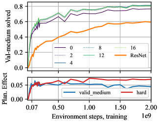
Figure 1: Top: Proportion of medium-difficulty validation levels solved vs. environment steps used in training. Curves show the RNN’s performance with a specific number of forced thinking steps at episode start, along with a ResNet baseline. Bottom: Estimated planning effect: the 8-steps minus the 0-steps curve. We see that reasoning emerges in the first 70M steps and keeps increasing for the hard levels, but decreases for medium levels.

1 Introduction

In many tasks, performance of both humans and sufficiently advanced neural networks (NNs) improves with more reasoning: whether giving a human more time to think before taking a chess move, or prompting a large language model to reason step by step (Kojima et al., 2022). Thus, understanding reasoning in such NNs is key to predicting their behavior in novel situations.

Among other reasoning capabilities, goal-oriented reasoning is particularly relevant to AI alignment. So-called “mesa-optimizers” – AIs that have learned to pursue goals through internal reasoning (Hubinger et al., 2019) – may internalize goals different from that given by the training objective, leading to harmful misgeneralization (Di Langosco et al., 2022; Shah et al., 2022).

This paper presents a 1.29M parameter recurrent neural network (RNN) that clearly benefits from extra time to reason. Following Guez et al. (2019), we train a convolutional LSTM to play Sokoban, a challenging puzzle game that remains a benchmark for planning algorithms (Peters et al., 2023) and reinforcement learning (Chung et al., 2024).

We believe understanding this RNN is a useful first step towards understanding reasoning in sophisticated neural networks. The network is complex enough to be interesting: it reasons in a challenging environment and benefits from extra thinking time. At the same time, it is simple enough to be tractable to reverse engineer with current mechanistic interpretability techniques, owing to its small size and relatively straightforward behavior.

We make three key contributions. First, we replicate and open-source an RNN whose performance improves with thinking time (Guez et al., 2019). Second, we analyze its training dynamics, finding that the thinking-time behavior emerges early in training and is incentivized by the setup (Figure 1, Sections 3 and 4.1). Third, we conduct a detailed empirical analysis of the network’s behavior. We quantitatively investigate how increased thinking changes network behavior (Section 3), showing that it reduces myopic actions (Figure 5). Furthermore, we present case studies of planning behavior that suggest the RNN naturally takes time to think (Section 4), which may explain the reduced planning effect on medium levels (Figure 1).

2 Training the test subject

We closely follow the setup from Guez et al. (2019), using the IMPALA (Espeholt et al., 2018) reinforcement learning (RL) algorithm with Guez et al.’s Deep Repeating ConvLSTM (DRC) recurrent architecture, as well as a ResNet. We open-source both the trained networks and training code.

Dataset.

Sokoban is a grid puzzle game with walls, floors, movable boxes, and target tiles. The player’s goal is to push all boxes onto target tiles while navigating walls. We use the Boxoban dataset (Guez et al., 2018), consisting of $10\times 10$ procedurally generated Sokoban levels, each with 4 boxes and targets. The edge tiles are always walls, so the playable area is $8\times 8$. Boxoban separates levels into train, validation and test sets, with three difficulty levels: unfiltered, medium, and hard. Guez et al. (2019) generated these by filtering levels that cannot be solved by progressively better-trained DRC networks, so easier sets occasionally contain difficult levels. In this paper, we use unfiltered-train (900k levels) to train networks. To evaluate them, we use unfiltered-test (1k levels), medium-validation (50k levels), and hard ($\sim$3.4k levels), which do not overlap.

Environment.

The observations are $10\times 10$ RGB images, normalized by dividing each component by 255. Each type of tile is represented by a pixel of a different color (Schrader, 2018). See Figure 6 for examples. The player can move in cardinal directions (Up, Down, Left, Right). The reward is -0.1 per step, 1 for putting a box on a target, -1 for removing a box, and 10 for finishing the level. To avoid strong time correlations during learning, each episode resets at a uniformly random length between 91 and 120 time steps.

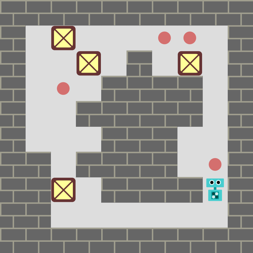
Figure 2: Left: A Sokoban level from the hard set. Right: the same level as the NN sees it, one pixel per tile. Walls are black, boxes are brown, targets are pink and the robot is green.

$\text{DRC}(D,N)$ architecture.

Guez et al. (2019) introduced the Deep Repeating ConvLSTM (DRC), whose core consists of $D$ convolutional LSTM layers with 32 channels and $3\times 3$ filters, each applied $N$ times per time step. Our $\text{DRC}(3,3)$ – or just DRC for brevity – has $1.29$M parameters. Before the LSTM core, two convolutional layers (without nonlinearity) encode the observation with $4\times 4$ filters.

The LSTM core uses $3\times 3$ convolutional filters, and a nonstandard tanh on the output gate (Jozefowicz et al., 2015). Unlike the original ConvLSTM (Shi et al., 2015), the input to each layer of a DRC consists of several concatenated components:

• The encoded observation is fed into each layer.

• To allow spatial information to travel fast in the ConvLSTM layers, we apply pool-and-inject by max- and mean-pooling the previous step’s hidden state. We linearly combine these values channel-wise before feeding them as an input to the next step.

• To avoid convolution edge effects from disrupting the LSTM dynamics, we feed in a $12\times 12$ channel with zeros on the inside and ones on the boundary. Unlike the other inputs, this one is not zero-padded, maintaining the output size.

ResNet architecture.

This is a convolutional residual neural network, also from Guez et al. (2019). It serves as a non-recurrent baseline that can only think during the forward pass (no ability to think for extra steps) but is nevertheless good at the game. The ResNet consists of 9 blocks, each with $4\times 4$ convolutional filters. The first two blocks have 32 channels, and the others have 64. Each block consists of a convolution, then two (relu, conv) sub-blocks, which each split off and are added back to the trunk. The ResNet has $3.07$M parameters.

Value and policy heads.

After the convolutions, an affine layer projects the flattened spatial output into 256 hidden units. We then apply a ReLU and two different affine layers: one for the actor (policy) and one for the critic (value function).

RL training.

We train each network for 2.003 billion environment steps using IMPALA (Espeholt et al., 2018; Huang et al., 2023). For each training iteration, we collect 20 transitions on 256 actors using the network parameters from the previous iteration, and simultaneously take a gradient step. We use a discount rate of $\gamma=0.97$ and V-trace $\lambda=0.5$. The value and entropy loss coefficients are $0.25$ and $0.01$. We use the Adam optimizer with a learning rate of $4\cdot 10^{-4}$, which linearly anneals to $4\cdot 10^{-6}$ at the end of training. We clip the gradient norm to $2.5\cdot 10^{-4}$. Our hyperparameters are mostly the same as Guez et al. (2019); see Appendix A.

A* solver.

We used the A* search algorithm to obtain optimal solutions to each Sokoban puzzle. The heuristic was the sum of the Manhattan distances of each box to its nearest target. Solving a single level on one CPU takes anywhere from a few seconds to 15 minutes.

3 Quantitative behavior analysis

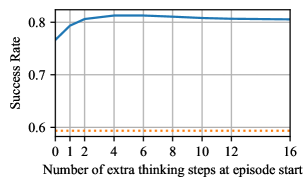
Figure 3: Proportion of medium-difficulty validation levels solved by DRC with $x$ time steps to think. The dotted line shows the ResNet’s solve proportion. The proportion of solved levels increases with thinking time, but only up to 6 steps.

3.1 Recurrent networks are better at Sokoban

After training both the recurrent $\text{DRC}(3,3)$ network and feed-forward ResNet for 2B environment transitions, the $\text{DRC}(3,3)$ network is able to solve $99.3\%$ of unfiltered test levels, while the ResNet solves only $97.9\%$. This gap is particularly notable given that the ResNet has more than double the parameters of the $\text{DRC}(3,3)$ network, so the ResNet has more model capacity and sequential thinking time. These results are consistent with Guez et al. (2019), see Appendix B.

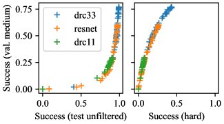
Figure 10: Success rate on datasets of various difficulty, for various checkpoints of each architecture. This deviates very little from a curve, which shows that ResNets and DRCs which are equally good at the easier sets are also equally good at the harder sets. Perhaps DRC(1,1) is a slight exception, but it also performs much worse than the others overall (see Figure 8).

The performance gap widens when considering just the hard levels, of which the $\text{DRC}(3,3)$ network solves $42.8\%$ and the ResNet $26.2\%$. Counterintuitively, we find that – controlling for performance on the unfiltered test set – recurrent networks are not comparatively better at harder levels than the ResNet. Figure 10 plots the performance of model checkpoints on the unfiltered test set against medium-difficulty and hard levels. We find that both model architectures follow the same curve: the recurrent $\text{DRC}(3,3)$ network is further to the right, but follows the same trend.

3.2 Thinking time improves performance

We find the performance of our trained $\text{DRC}(3,3)$ improves given additional thinking time, replicating Guez et al. (2019). We evaluate the DRC network on all medium-difficulty validation levels. To induce thinking time, we repeat the initial environment observation $n$ times while advancing the DRC hidden state, then let the DRC policy act normally. Figure 3 shows the DRC’s performance for $n\in\{0,1,2,4,6,8,10,12,16\}$ steps, alongside the ResNet baseline. The DRC’s success rate improves from $76.6\%$ to $81.3\%$ with more thinking steps, with peak performance at 6 steps. The effect ($4.7\%$ difference) is comparable to that observed by Guez et al. ($4.5\%$).

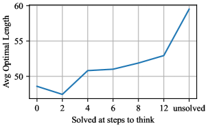
Figure 4: Average optimal solution length of levels grouped by the number of thinking steps at which the level is first solved. Each of the 50,000 medium-difficulty validation levels is assigned to a group. Optimal solution length is a proxy for difficulty, and we can see that levels which take longer to solve tend to be harder.

3.3 Planning emerges early in training

Figure 1 shows the performance of the DRC on the medium-difficulty validation levels by training step. We see the DRC rapidly acquires a strong planning effect by 70M environment steps. This effect strengthens on the hard levels as training progresses, but slowly weakens for medium-difficulty levels. This suggests that the training setup and loss function reinforce the planning effect for harder levels and disincentivize it for levels that are comparatively easier.

3.4 Do difficult levels benefit more from thinking?

The A* solver gives us two proxies for the difficulty of a level: the length of the optimal solution, and the number of nodes it had to expand to find a solution. Figure 4 shows a positive correlation between the A* optimal solution length ($y$-axis) and the number of DRC thinking steps $n$ needed to solve a level ($x$-axis). In other words, taking extra more thinking time helps solve harder levels.

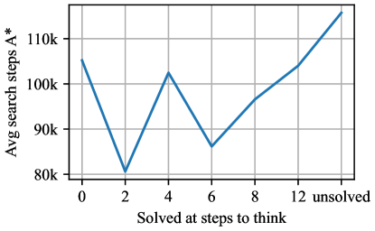
Figure 11: Number of thinking steps required to solve the level vs. number of nodes A* needs to expand to solve it. The trend is somewhat increasing but much less clear, indicating different heuristics used by the NN and A*.

On the other hand, Figure 11 (Appendix D) finds only a weakly positive correlation between the expanded nodes proxy and required thinking steps $n$, with results noisy for smaller $n$. We speculate that the ‘expanded nodes’ proxy metric is only weakly related to required $n$ due to the DRC having different heuristics than the one we use for A*, whereas the optimal solution length does not depend on heuristics.

Table 1: Levels at 6 thinking steps.

Level categorization	Percentage
Solved, previously unsolved	6.87
Unsolved, previously solved	2.23
Solved, with better returns	18.98
Solved, with the same returns	50.16
Solved, with worse returns	5.26
Unsolved, with same or better returns	15.14
Unsolved, with worse returns	1.36

3.5 Other consequences of DRC thinking time

While Figure 3 shows that the DRC can solve many more levels when given thinking steps at the beginning of an episode, in this section, we explore how the network’s behavior changes with thinking time, and if this has significant effects besides solving more levels.

Thinking makes the DRC “patient.”

One hypothesis is that, without the extra thinking steps, the DRC sometimes comes up with a greedy solution for some of the boxes and executes it right away. This puts some boxes into the wrong targets, and makes the puzzle unsolvable. Since the training signal penalizes every step it takes to solve the puzzle, it could be optimal for a bounded rational agent to avoid thinking and be “impatient” in this way: the agent may accumulate more return on average by being “impatient” and quickly solving most levels even if it sometimes errs by taking actions that make it impossible to solve other levels.

For $n$ thinking steps, Figure 5 plots the average number of steps (time-to-box) until each of 4 boxes gets on a target, in the order in which they do so. The results support the hypothesis: levels that are solved at 6 thinking steps but unsolved at 0 thinking steps show increased time-to-box for boxes 1-3 but decreased time for box 4 (Figure 5(b)). In contrast, averaged across all levels times go down for all boxes with increased thinking (Figure 5(a)).

Thinking often improves solutions for already-solved levels, but is sometimes harmful.

Table 1 shows that an additional 6 thinking steps solves 6.87% of previously unsolved levels – but at the cost of no longer being able to solve 2.23% of previously solved levels, for a total improved solution rate of 4.64%. In addition to improving the solution rate, additional thinking improves returns on average by shortening solution length in 18.98% of episodes, consistent with the decreased timesteps to place boxes shown in Figure 5(a). However, the effect is inconsistent: most episodes show no change in returns, with returns even decreasing in 5.26% of episodes. Overall, extra thinking steps are not always beneficial but, on balance, they let the DRC solve more levels or improve return on already solved levels.

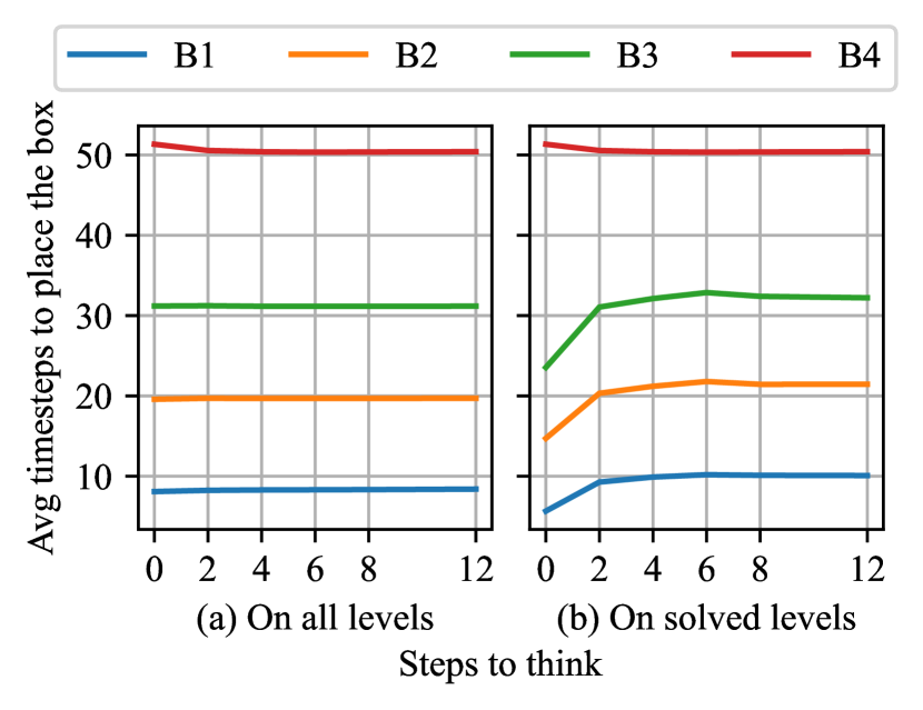
Figure 5: Average time step to place each box $Bi$ on target for different thinking steps. (a) Averages across all levels where the box $Bi$ is placed on target by DRC with $n$ thinking steps. If box $Bi$ is not placed (on unsolved levels) we ignore the box, but we keep the other boxes in the level. (b) Averages for all levels solved by $6$ thinking steps but not solved by $0$ thinking steps.

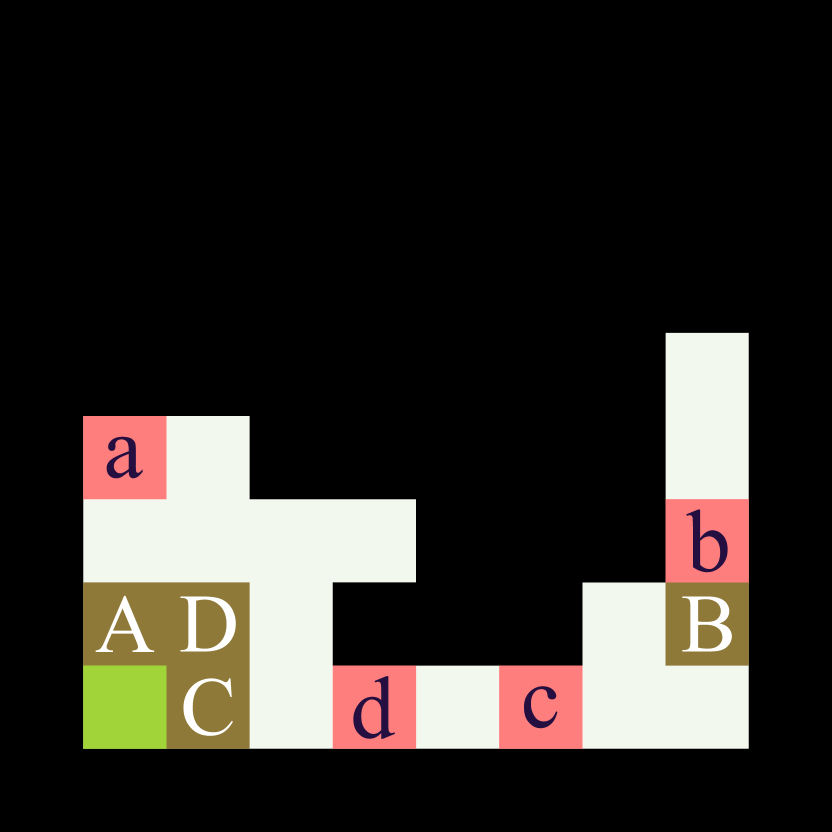
(a) file 0, level 18
unsolved $\overset{\text{think}}{\rightarrow}$ solved

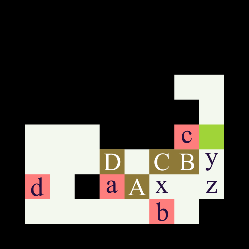
(b) file 0, level 53
$\overset{\text{think}}{\rightarrow}$ solved faster

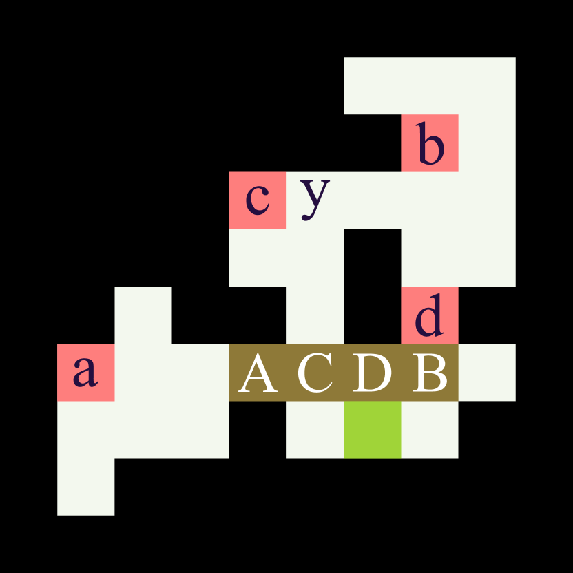
(c) file 0, level 153
$\overset{\text{think}}{\rightarrow}$ solved slower

Figure 6: Case studies of three medium-validation levels demonstrating different behaviors after 6 thinking steps. Colors are as in Figure 2. Boxes and targets are paired in upper- and lower-case letters respectively, such that the DRC’s best solution places boxes on targets in alphabetical order. Videos available at this https URL; see Section 4 for behavior descriptions. Levels solved faster obtain higher return as the agent incurs the per-step penalty fewer times.

4 Case studies: how does thinking change behavior?

To gain a deeper understanding of the DRC networks’ behavior, we examine an example from each of three categories from Table 1: a solved, previously unsolved level; a level on which the DRC improved its return with extra thinking (solved faster); and a level on which the return worsens (solved slower). We select an illustrative example of each category from the first ten examples by level index.

Thinking lets the DRC solve: Figure 6(a).

In the no-thinking condition, the DRC first pushes box $C$ one square to the right. It then goes back to push $A$ to $a$, but it is too late: it is now impossible to push box $B$ onto $b$. The network pushes $C$ onto $c$, then $D$ onto $d$ and then remains mostly still. In contrast, after thinking, the DRC pushes $A$ to $a$ first, which lets it solve the level.

Thinking speeds up solving: Figure 6(b).

In the no-thinking condition, the DRC spends many steps going back and forth before pushing any boxes. First it goes down to $y$, then up to $c$, then down onto $z$, back up to $y$ and to $z$ again. It then proceeds to solve the rest of the puzzle correctly: push box $A$ onto $a$, prepare box $B$ on $x$ and box $C$ where $B$ originally was, push in boxes $B,C$ and finally $D$. In the thinking condition, the DRC makes a beeline for $A$ and then plays the exact same solution.

Thinking slows down solving: Figure 6(c).

In the no-thinking condition, the DRC starts by pushing box $C$ into position $y$, then pushes boxes $A,B$. On the way back down, ther DRC pushes $C$ onto $c$ and finally $D$ onto $d$. In contrast, after thinking for a bit, the DRC goes the other way and starts by pushing $B$ onto $b$. The solution is the same after that: $A$, $C$, then $D$; but the NN has wasted time trekking back from $B$ to $A$.

4.1 Hypothesis: the DRC ‘paces’ to get thinking time

The second case study above found the DRC sometimes moves around in cycles without touching any box. One hypothesis for why this occurs is that the DRC is using the extra steps to come up with a plan to solve the episode. To test this, we can check whether cycles in the game state occur more frequently near the start of the episode, and whether deliberately giving the DRC thinking time makes it stop going in cycles.

Consistent with this hypothesis, Figure 7 (left) shows the majority of cycles start within the first 5 steps of the episode, and (right) forcing it to think for six steps makes about 75% of these cycles disappear.

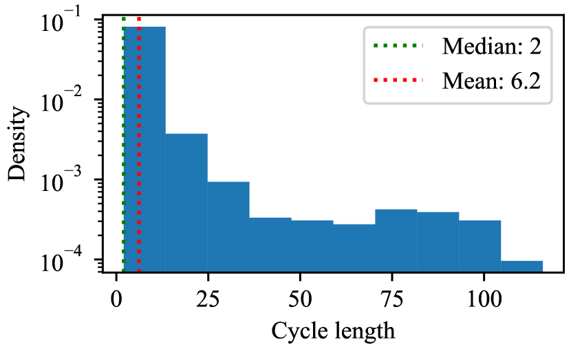
(a) Cycle length distribution

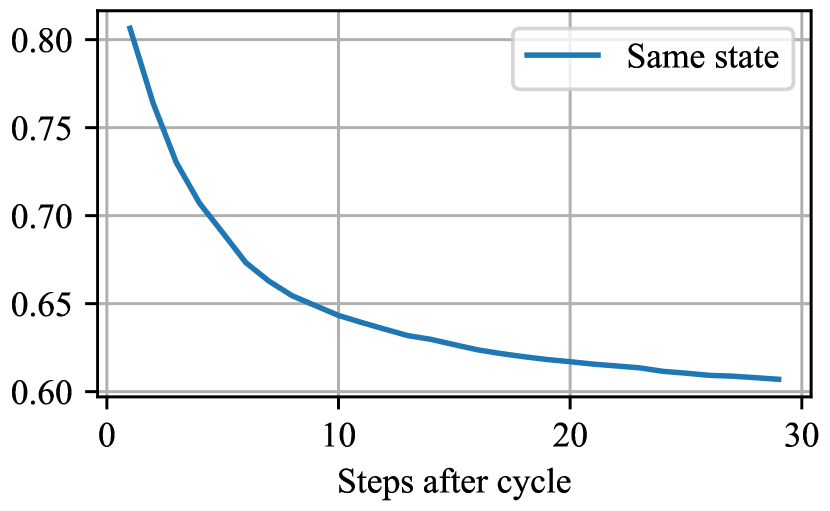
(b) with cycles from all levels

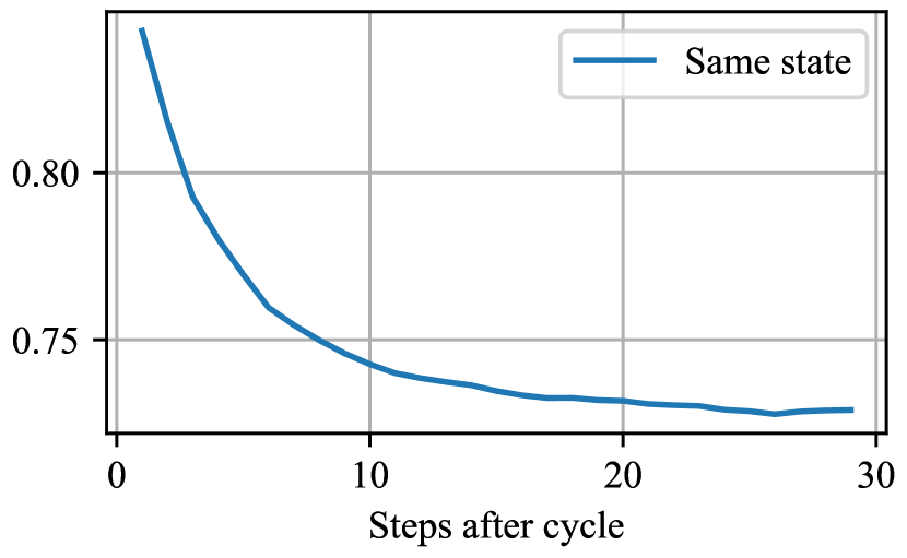
(c) with cycles from those levels that were solved by the agent

Figure 9: We replace N-length cycles with N thinking steps and checking for the same state after some timesteps. (a) A histogram of cycle lengths in the medium-validation set. (b, c) After replacing a cycle with the same length in thinking steps, are all the states the same for the next $x$ steps?

The episode start is not the only time at which the DRC moves in cycles. Figure 9 shows that replacing an $n$-length cycle with $n$ thinking steps leads the NN to have the exact same behavior for at least 60% of levels, for at least 30 steps after the cycle. For context, the median solution length for train-unfiltered is exactly 30 steps. Additionally, in $82.39\%$ of cases, doing this prevents cycles from starting in the $n$ steps after the thinking-steps conclude (Appendix C).

Why does this behavior emerge during training? Thinking is useful for achieving higher return, so it should be reinforced. But it also has a cost, -0.1 per step, so it should be discouraged in easy levels that do not need the computation. We speculate that, as training advances and heuristics get tuned, the DRC needs to think in fewer levels, and it is better at knowing when it needs to pace. This would also explain why, after many training steps, the DRC network begins to benefit less from additional thinking steps at the start of the episode in Figure 1: the DRC finds levels easier and also knows to pace when thinking is needed.

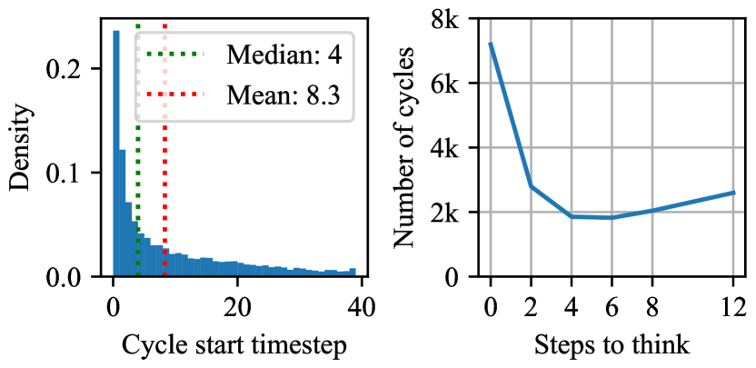
Figure 7: Left: Histogram of cycle start times on the medium-difficulty validation levels. Right: Total number of cycles the agent takes in the first 5 steps across all episodes in medium-difficulty validation levels with $n$ initial thinking steps.

5 Related work

Interpretability of agents and world models.

Several works have attempted to find the mechanism by which a simple neural network does planning in mazes (Ivanitskiy et al., 2023; Mini et al., 2023), gridworlds (Bloom & Colognese, 2023), and graph search (Ivanitskiy et al., 2023). We believe the DRC we present is a clearer example of an agent than what these works focus on, and should be similarly possible to interpret.

Other works have found emergent world models in sequence-prediction (Li et al., 2023) and navigation (Wijmans et al., 2023) neural networks.

Goal misgeneralization and mesa-optimizers for alignment.

From the alignment perspective, AIs optimizing monomaniacally for a goal have long been a concern (e.g. Yudkowsky, 2006; Omohundro, 2008; see the preface of Russell, 2019). In a machine learning paradigm (Hubinger et al., 2019), the goal of the training system is not necessarily optimized; instead, the NN may optimize for a related or different goal (Di Langosco et al., 2022; Shah et al., 2022), or for no goal at all.

Chain-of-thought faithfulness.

Large language models (LLMs) use chain of thought, but are they faithful to it or do they think about their future actions in other ways (Lanham et al., 2023; Pfau et al., 2024)? One could hope that LLMs perform all long-term reasoning in plain English, allowing unintended human consequences to be easily monitored, as in Scheurer et al. (2023).

Reasoning neural network architectures.

Many papers try to enhance NN thinking by altering the training setup or architecture (Bansal et al., 2022; Graves, 2016; Chung et al., 2024).

Ethical treatment of AIs.

Do AIs deserve moral consideration? Schwitzgebel & Garza (2015) argue that very human-like AIs are conceivable and clearly deserve rights. Tomasik (2015) suggests that most AIs deserve at least a little consideration, like biological organisms of any species (Singer, 2004). But what does it mean to treat an AI ethically? Daswani & Leike (2015) argue that the way to measure pleasure and pain in a reinforcement learner is not by its absolute amount of return, but rather by the temporal difference (TD) error: the difference between its expectations and the actual return it obtained. If the internals of the NN have a potentially different objective (Hubinger et al., 2019; Di Langosco et al., 2022), then the TD error should come from a place other than the critic. This paper is an early step toward finding the learned-reward internal TD error, if it exists.

6 Conclusion

We have developed and open-sourced a model organism for understanding reasoning in neural networks. In addition, we contribute a detailed empirical analysis of this network’s behavior. We believe this work will prove useful to the interpretability, alignment, and ethical treatment of AIs.

First, we have trained a DRC recurrent network that plays Sokoban and benefits from additional thinking steps at test time, replicating Guez et al. (2019).

Second, we have shown that thinking for longer helps solve harder levels, and makes the DRC better at levels that require longer-sighted behavior. Without intervention, thinking sometimes takes the form of the DRC ‘pacing’ at the beginning or middle of the episode, in a way which can be substituted by repeating the same input. This suggests the network is deliberately using more computation by pacing.

Finally, we have shown that the training setup incentivizes the planning effect at the start. We find that planning is disincentivized later, but only for easier levels. We offer a hypothesis about why the training process disincentivizes the planning effect: the NN finds levels easier (needs less thinking), and also learns when to do the thinking it needs (via pacing).

7 Acknowledgements

We would like to thank ChengCheng Tan for editing this paper, Philip Quirke for project management, and the rest of the FAR team for general support. We also thank Maximilian Li, Alex F. Spies, and anonymous reviewers for improving the paper with their comments and edits. We are also very grateful for the many questions about their RL setup that Arthur Guez and Timothy Lillicrap answered, as well as inspiration from Stephen Chung and Scott Goodfriend.

Appendix A Training hyperparameters

All networks were trained with the same hyperparameters, which were tuned on a combination of the ResNet and the $\text{DRC}(3,3)$. These are almost exactly the same as Guez et al. (2019), allowing for taking the mean of the per-step loss instead of the sum.

Loss.

The value and entropy coefficients are 0.25 and 0.01 respectively. It is very important to not normalize the advantages for the policy gradient step.

Gradient clipping and epsilon

The original IMPALA implementation, as well as Huang et al. (2023), sum the per-step losses. We instead average them for more predictability across batch sizes, so we had to scale down some parameters by a factor of $1/640$: Adam $\epsilon$, gradient norm for clipping, and L2 regularization).

Weight initialization.

We initialize the network with the Flax (Heek et al., 2023) default: normal weights truncated at 2 standard deviations and scaled to have standard deviation $\sqrt{1/\text{fan\_in}}$. Biases are initialized to 0. The forget gate of LSTMs has 1 added to it (Jozefowicz et al., 2015). We initialize the value and policy head weights with orthogonal vectors of norm 1. Surprisingly, this makes the variance of these unnormalized residual networks decently close to 1.

Adam optimizer.

As our batch size is medium-sized, we pick $\beta_{1}=0.9$, $\beta_{2}=0.99$. The denominator epsilon is $\epsilon=1.5625\cdot 10^{-7}$. Learning rate anneals from $4\cdot 10^{-4}$ at the beginning to $4\cdot 10^{-6}$ at 2,002,944,000 steps.

L2 regularization.

In the training loss, we regularize the policy logits with L2 regularization with coefficient $1.5625\times 10^{-6}$. We regularize the actor and critic heads’ weights with L2 at coefficient $1.5625\times 10^{-8}$. We believe this has essentially no effect, but we left it in to more closely match Guez et al. (2019).

Software.

We base our IMPALA implementation on Cleanba (Huang et al., 2023). We implemented Sokoban in C++ using Envpool (Weng et al., 2022) for faster training, based on gym-sokoban (Schrader, 2018).

A.1 Number of training steps

In the body of the paper we state the networks train for $2.003\text{B}$ steps. The exact number is $2\,002\,944\,000$ steps. Our code and hyperparameters require that the number of environment steps be divisible by $5\,120=256\text{ environments}\times 20\text{ steps collected}$, because that is the number of steps in one iteration of data collection.

However, $2\text{B}$ is divisible by $5\,120$, so there is no need to add a remainder. We noticed this mistake once the networks already have trained. It is not worth retraining the networks from scratch to fix this mistake.

At some point in development, we settled on $80\,025\,600$ to approximate $80\text{M}$ while being divisible by $256\times 20$ and $192\times 20$. Perhaps due to error, this mutated into $1\,001\,472\,000$ as an approximation to $1\text{B}$, which directly leads to the number we used.

Appendix B Learning curve comparison

It is difficult to fully replicate the results by Guez et al. (2019). Chung et al. (2024) propose an improved method for RL in planning-heavy domains. They employ the IMPALA $\text{DRC}(3,3)$ as a baseline and plot its performance in Chung et al. (2024, Figure 5). They plot two separate curves for $\text{DRC}(3,3)$: that from Guez et al. (2019), and a decent replicated baseline. The baseline is considerably slower to learn and peaks at lower performance.

We did not innovate in RL, so were able to spend more time on the replication. We compare our replication to Guez et al. (2019) in Figure 8, which shows that the learning curves for $\text{DRC}(3,3)$ and ResNet are compatible, but not the one for DRC(1,1). Our implementation also appears much less stable, with large error bars and large oscillations over time. We leave addressing that to future work.

The success rate in Figure 8 is computed over 1024 random levels, unlike the main body of the paper. Table 3 reports test and validation performance for the DRC and ResNet seeds which we picked for the paper body.

The parameter counts (Table 2) are very different from what Guez et al. (2019) report. In private communication with the authors, we confirmed that our architecture has a comparable number of parameters, and some of the originally reported numbers are a typographical error.

Table 2: Parameter counts for each architecture.

Architecture	Parameter count
$\text{DRC}(3,3)$	1,285,125	(1.29M)
DRC(1,1)	987,525	(0.99M)
ResNet:	3,068,421	(3.07M)

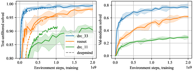
Figure 8: Success rate for Test-unfiltered and Validation-medium levels vs. environment steps of training. Each architecture has 5 random seeds, the solid line is the pointwise median and the shaded area spans from the minimum to the maximum. The dotted lines are data for the performance of architectures extracted from the (Guez et al., 2019) PDF file. The values are slightly different from what Figures 1 and 3 report because they are calculated on a random sample of 1024 levels (24 levels are repeated for test-unfiltered).

Table 3: Success rate and return of DRC and ResNet on the unfiltered test set at various training environment steps.

Training Env	Test Unfiltered				Valid Medium
Steps	ResNet		DRC(3, 3)		ResNet		DRC(3, 3)
	Success	Return	Success	Return	Success	Return	Success	Return
100M	87.8	8.13	95.4	9.58	18.6	-6.59	47.9	-0.98
500M	93.1	9.24	97.9	10.21	39.7	-2.64	66.6	2.62
1B	95.4	9.75	99.2	10.47	50.0	-0.64	70.4	3.40
2B	97.9	10.29	99.3	10.52	59.4	1.16	76.6	4.52

Appendix C Additional cycles investigation

We run the DRC(3,3) on medium-validation levels and record where cycles in the game state happen. We prune out the redundant cycles that visit the same states as a given cycle. There are in total 13702 non-redundant cycles. For each cycle, if it is of length $N$, we replace it with $N$ steps of thinking, and measure what happens. In 86.74% of cases the DRC(3,3) does not immediately start going in cycles after the thinking time. That is, no cycle begins in the step after thinking time. In 82.39% of cases this persists for the next $N$ time steps: no cycles start in the $N$ steps after thinking.

Appendix D Additional quantitative behavior figures

References

- Bansal et al. (2022) Bansal, A., Schwarzschild, A., Borgnia, E., Emam, Z., Huang, F., Goldblum, M., and Goldstein, T. End-to-end algorithm synthesis with recurrent networks: Extrapolation without overthinking. In Oh, A. H., Agarwal, A., Belgrave, D., and Cho, K. (eds.), Advances in Neural Information Processing Systems, 2022. URL https://openreview.net/forum?id=PPjSKy40XUB.
- Bloom & Colognese (2023) Bloom, J. and Colognese, P. Decision transformer interpretability, 2023. URL https://www.lesswrong.com/posts/bBuBDJBYHt39Q5zZy/decision-transformer-interpretability.
- Chung et al. (2024) Chung, S., Anokhin, I., and Krueger, D. Thinker: Learning to plan and act. Advances in Neural Information Processing Systems, 36, 2024. URL https://openreview.net/forum?id=mumEBl0arj.
- Daswani & Leike (2015) Daswani, M. and Leike, J. A definition of happiness for reinforcement learning agents. arXiv, 2015. URL http://arxiv.org/abs/1505.04497v1.
- Di Langosco et al. (2022) Di Langosco, L. L., Koch, J., Sharkey, L. D., Pfau, J., and Krueger, D. Goal misgeneralization in deep reinforcement learning. In International Conference on Machine Learning, pp. 12004–12019. PMLR, 2022. URL https://proceedings.mlr.press/v162/langosco22a.html.
- Espeholt et al. (2018) Espeholt, L., Soyer, H., Munos, R., Simonyan, K., Mnih, V., Ward, T., Doron, Y., Firoiu, V., Harley, T., Dunning, I., Legg, S., and Kavukcuoglu, K. IMPALA: Scalable distributed deep-RL with importance weighted actor-learner architectures. arXiv, 2018. URL http://arxiv.org/abs/1802.01561v3.
- Graves (2016) Graves, A. Adaptive computation time for recurrent neural networks. arXiv, 2016. URL http://arxiv.org/abs/1603.08983v6.
- Guez et al. (2018) Guez, A., Mirza, M., Gregor, K., Kabra, R., Racaniere, S., Weber, T., Raposo, D., Santoro, A., Orseau, L., Eccles, T., Wayne, G., Silver, D., Lillicrap, T., and Valdes, V. An investigation of model-free planning: boxoban levels, 2018. URL https://github.com/deepmind/boxoban-levels/.
- Guez et al. (2019) Guez, A., Mirza, M., Gregor, K., Kabra, R., Racanière, S., Weber, T., Raposo, D., Santoro, A., Orseau, L., Eccles, T., Wayne, G., Silver, D., and Lillicrap, T. An investigation of model-free planning. arXiv, 2019. URL http://arxiv.org/abs/1901.03559v2.
- Heek et al. (2023) Heek, J., Levskaya, A., Oliver, A., Ritter, M., Rondepierre, B., Steiner, A., and van Zee, M. Flax: A neural network library and ecosystem for JAX, 2023. URL http://github.com/google/flax.
- Huang et al. (2023) Huang, S., Weng, J., Charakorn, R., Lin, M., Xu, Z., and Ontañón, S. Cleanba: A reproducible and efficient distributed reinforcement learning platform, 2023. URL https://arxiv.org/abs/2310.00036.
- Hubinger et al. (2019) Hubinger, E., van Merwijk, C., Mikulik, V., Skalse, J., and Garrabrant, S. Risks from learned optimization in advanced machine learning systems, 2019. URL https://arxiv.org/abs/1906.01820.
- Ivanitskiy et al. (2023) Ivanitskiy, M., Spies, A. F., Räuker, T., Corlouer, G., Mathwin, C., Quirke, L., Rager, C., Shah, R., Valentine, D., Behn, C. D., Inoue, K., and Fung, S. W. Linearly structured world representations in maze-solving transformers. In UniReps: the First Workshop on Unifying Representations in Neural Models, 2023. URL https://openreview.net/forum?id=pZakRK1QHU.
- Jozefowicz et al. (2015) Jozefowicz, R., Zaremba, W., and Sutskever, I. An empirical exploration of recurrent network architectures. In Bach, F. and Blei, D. (eds.), International Conference on Machine Learning, volume 37 of Proceedings of Machine Learning Research, pp. 2342–2350, Lille, France, 07–09 Jul 2015. PMLR. URL https://proceedings.mlr.press/v37/jozefowicz15.html.
- Kojima et al. (2022) Kojima, T., Gu, S. S., Reid, M., Matsuo, Y., and Iwasawa, Y. Large language models are zero-shot reasoners. Advances in Neural Information Processing Systems, 35:22199–22213, 2022. URL https://openreview.net/pdf?id=e2TBb5y0yFf.
- Lanham et al. (2023) Lanham, T., Chen, A., Radhakrishnan, A., Steiner, B., Denison, C., Hernandez, D., Li, D., Durmus, E., Hubinger, E., Kernion, J., et al. Measuring faithfulness in chain-of-thought reasoning. arXiv preprint arXiv:2307.13702, 2023. URL https://arxiv.org/abs/2307.13702.
- Li et al. (2023) Li, K., Hopkins, A. K., Bau, D., Viégas, F., Pfister, H., and Wattenberg, M. Emergent world representations: Exploring a sequence model trained on a synthetic task. In International Conference on Learning Representations, 2023. URL https://openreview.net/forum?id=DeG07_TcZvT.
- Mini et al. (2023) Mini, U., Grietzer, P., Sharma, M., Meek, A., MacDiarmid, M., and Turner, A. M. Understanding and controlling a maze-solving policy network. arXiv, 2023. URL http://arxiv.org/abs/2310.08043v1.
- Omohundro (2008) Omohundro, S. M. The basic AI drives. In Proceedings of the 2008 Conference on Artificial General Intelligence 2008: Proceedings of the First AGI Conference, pp. 483–492, NLD, 2008. IOS Press. ISBN 9781586038335.
- Peters et al. (2023) Peters, N. S., Alexa, M., and Neurotechnology, S. F. Solving sokoban efficiently: Search tree pruning techniques and other enhancements, 2023. URL https://doc.neuro.tu-berlin.de/bachelor/2023-BA-NiklasPeters.pdf.
- Pfau et al. (2024) Pfau, J., Merrill, W., and Bowman, S. R. Let’s think dot by dot: Hidden computation in transformer language models. arXiv, 2024. URL http://arxiv.org/abs/2404.15758v1.
- Russell (2019) Russell, S. Human compatible: artificial intelligence and the problem of control. Penguin, 2019.
- Scheurer et al. (2023) Scheurer, J., Balesni, M., and Hobbhahn, M. Large language models can strategically deceive their users when put under pressure. arXiv, 2023. URL http://arxiv.org/abs/2311.07590v3.
- Schrader (2018) Schrader, M.-P. B. gym-sokoban, 2018. URL https://github.com/mpSchrader/gym-sokoban.
- Schwitzgebel & Garza (2015) Schwitzgebel, E. and Garza, M. A defense of the rights of artificial intelligences. Midwest Studies In Philosophy, 39(1):98–119, 2015. doi: 10.1111/misp.12032. URL http://www.faculty.ucr.edu/~eschwitz/SchwitzPapers/AIRights-150915.htm.
- Shah et al. (2022) Shah, R., Varma, V., Kumar, R., Phuong, M., Krakovna, V., Uesato, J., and Kenton, Z. Goal misgeneralization: why correct specifications aren’t enough for correct goals. arXiv preprint arXiv:2210.01790, 2022. URL https://arxiv.org/abs/2210.01790.
- Shi et al. (2015) Shi, X., Chen, Z., Wang, H., Yeung, D.-Y., Wong, W.-K., and Woo, W.-c. Convolutional LSTM network: A machine learning approach for precipitation nowcasting. Advances in Neural Information Processing Systems, 28, 2015. URL https://proceedings.neurips.cc/paper_files/paper/2015/file/07563a3fe3bbe7e3ba84431ad9d055af-Paper.pdf.
- Singer (2004) Singer, P. Animal liberation. In Ethics: Contemporary Readings, pp. 284–292. Routledge, 2004.
- Tomasik (2015) Tomasik, B. A dialogue on suffering subroutines, 2015. URL https://longtermrisk.org/a-dialogue-on-suffering-subroutines/.
- Weng et al. (2022) Weng, J., Lin, M., Huang, S., Liu, B., Makoviichuk, D., Makoviychuk, V., Liu, Z., Song, Y., Luo, T., Jiang, Y., Xu, Z., and Yan, S. EnvPool: A highly parallel reinforcement learning environment execution engine. In Koyejo, S., Mohamed, S., Agarwal, A., Belgrave, D., Cho, K., and Oh, A. (eds.), Advances in Neural Information Processing Systems, volume 35, pp. 22409–22421. Curran Associates, Inc., 2022. URL https://openreview.net/forum?id=BubxnHpuMbG.
- Wijmans et al. (2023) Wijmans, E., Savva, M., Essa, I., Lee, S., Morcos, A. S., and Batra, D. Emergence of maps in the memories of blind navigation agents. In International Conference on Learning Representations, 2023. URL https://openreview.net/forum?id=lTt4KjHSsyl.
- Yudkowsky (2006) Yudkowsky, E. Artificial intelligence as a positive and negative factor in global risk. In Bostrom, N. and ĆirkoviĆ, M. M. (eds.), Artificial Intelligence as a positive and negative factor in global risk, 2006. URL https://api.semanticscholar.org/CorpusID:2629818.