Concentration and limit of large random matrices with given margins

Abstract.

We study large random matrices with i.i.d. entries conditioned to have prescribed row and column sums (margin). This problem has rich connections to relative entropy minimization, Schrödinger bridge, the enumeration of contingency tables, and random graphs with given degree sequences. We show that such margin-constrained random matrix is sharply concentrated around a certain deterministic matrix, which we call the typical table. Typical tables have dual characterizations: (1) the expectation of the random matrix ensemble with minimum relative entropy from the base model constrained to have the expected target margin, and (2) the expectation of the maximum likelihood model obtained by rank-one exponential tilting of the base model. The structure of the typical table is dictated by two dual variables, which give the maximum likelihood estimates of the tilting parameters. Based on these results, for a sequence of "tame" margins that converges in $L^{1}$ to a limiting continuum margin as the size of the matrix diverges, we show that the sequence of margin-constrained random matrices converges in cut norm to a limiting kernel, which is the $L^{2}$-limit of the corresponding rescaled typical tables. The rate of convergence is controlled by how fast the margins converge in $L^{1}$. We derive several new results for random contingency tables from our general framework.

1. Introduction

In this paper, we are interested in the structure of random matrix conditions to have prescribed row and column sums. Let $\mu$ be a (not necessarily a probability) measure on $\mathbb{R}$, and let

(1.1) $$A:=\inf\{{\rm supp}(\mu)\}\leq\sup\{{\rm supp}(\mu)\}=:B.$$

We allow for the possibility that $A=-\infty$, and/or $B=\infty$. When $\mu$ is a probability measure, then the base model for the $m\times n$ random matrix is $X=(X_{ij})$ where the entries are independent and identically distributed as $\mu$. In this case, we write $X\sim\mu^{\otimes(m\times n)}$.

Let $\mathbf{x}=(x_{ij})$ be an $m\times n$ matrix of real entries. We define the row margin of $\mathbf{x}$ as vector $r(\mathbf{x}):=(r_{1}(\mathbf{x}),\dots,r_{m}(\mathbf{x}))$ with $r_{i}(\mathbf{x}):=\sum_{j=1}^{n}x_{ij}$; the column margin of $\mathbf{x}$ is a vector $c(\mathbf{x}):=(c_{1}(\mathbf{x}),\dots,c_{n}(\mathbf{x}))$ with $c_{j}(\mathbf{x}):=\sum_{i=1}^{m}x_{ij}$. We call the pair $(r(\mathbf{x}),c(\mathbf{x}))$ the margin of $\mathbf{x}$. For each $\rho\geq 0$, we let

(1.2) $$\mathcal{T}_{\rho}(\mathbf{r},\mathbf{c}):=\left\{\mathbf{x}\in\mathbb{R}^{m\times n}\,:\,\textup{$\lVert r(\mathbf{x})-\mathbf{r}\rVert_{1}\leq\rho$ and $\lVert c(\mathbf{x})-\mathbf{c}\rVert_{1}\leq\rho$ }\right\}$$

denote the set of all $m\times n$ real matrices whose margin is within $L^{1}$ distance $\rho$ from the prescribed margin $(\mathbf{r},\mathbf{c})$. The transportation polytope with margin $(\mathbf{r},\mathbf{c})$ is the set $\mathcal{T}(\mathbf{r},\mathbf{c}):=\mathcal{T}_{0}(\mathbf{r},\mathbf{c})$.

A fundamental question we investigate in this work is how a random matrix drawn from the base model behaves if we condition its margins to take prescribed values. Namely,

(1.3) If we condition $$X\sim\mu^{\otimes(m\times n)} \mathcal{T}_{\rho}(\mathbf{r},\mathbf{c})$$ on being in , how does it look like?

The above question still makes sense when $\mu$ is not a probability measure (e.g., counting measure on $\mathbb{N}$) under the following assumption:

(1.4) $$\int_{\mathcal{T}_{\rho}(\mathbf{r},\mathbf{c})}d\mu^{\otimes(m\times n)}(\mathbf{x})\in(0,\infty),$$

that is, the measure of $\mathcal{T}_{\rho}(\mathbf{r},\mathbf{c})$ under $\mu^{\otimes(m\times n)}$ is positive and finite. In this case we understand $X$ as being sampled from the probability measure obtained by normalizing $\mu^{\otimes(m\times n)}$ on $\mathcal{T}_{\rho}(\mathbf{r},\mathbf{c})$. Note that (1.3) is a random-matrix-analog of the well-studied problem of understanding the behavior of uniformly random graphs with a given degree sequence [17, 11]. As we will see later, it turns out that this problem is also closely related to the enumeration of contingency tables (nonnegative inter-valued matrices with prescribed margins) in combinatorics as well as relative entropy minimization (also known as the information projection) problems [24, 25].

Our high-level answer to the above question can be phrased as below from two complementary perspectives of minimum relative entropy and maximum likelihood:

1.

(Minimum Relative Entropy Perspective): The expectation of the random matrix ensemble with minimum relative entropy from the base model constrained to have the expected target margin $(\mathbf{r},\mathbf{c})$

2.

(Maximum Likelihood Perspective): The expectation of the maximum likelihood entrywise exponential tilting of the base model for margin $(\mathbf{r},\mathbf{c})$.

1.1. Statement of main results

To make the statements more precise, we introduce some notations.

Definition 1.1 (Exponential tilting).

Define the set $\Theta$ of all allowed tilting parameters for $\mu$:

(1.5) $$\Theta:=\Big{\{}\theta\in\mathbb{R}:\int e^{\theta x}d\mu(x)<\infty\Big{\}}.$$

Let $\Theta^{\circ}$ be the interior of $\Theta$. For any $\theta\in\Theta^{\circ}$, let $\mu_{\theta}$ denote the tilted probability measure given by

(1.6) $$\frac{d\mu_{\theta}}{d\mu}(x)=e^{\theta x-\psi(\theta)},\quad\psi(\theta):=\log\int e^{\theta x}d\mu(x).$$

Then we have $\mathbb{E}_{\mu_{\theta}}[X]=\psi^{\prime}(\theta)$ and $\operatorname{\textnormal{Var}}_{\mu_{\theta}}(X)=\psi^{\prime\prime}(\theta)>0$, so the function $\psi^{\prime}(.):\Theta^{\circ}\mapsto(A,B)$ is strictly increasing, and has a strictly increasing inverse $\phi(.):(A,B)\mapsto\Theta^{\circ}$ satisfying $\phi(\psi^{\prime}(\theta))=\theta$ for all $\theta\in\Theta^{\circ}$. For $\theta\in\Theta^{\circ}$, the relative entropy from $\mu$ to the tilted probability measure $\mu_{\theta}$ is

(1.7) $$D(\mu_{\theta}\lVert\mu):=\int_{x\in\mathbb{R}}\log\left(\frac{d\mu_{\theta}}{d\mu}(x)\right)\,d\mu_{\theta}(x)=\theta\psi^{\prime}(\theta)-\psi(\theta).$$

Throughout this paper, we assume the measure $\mu$ on $\mathbb{R}$ is so that the set $\Theta$ of tilting parameters in (1.5) is nonempty and not a singleton. Then it follows from Hölder’s inequality that $\Theta$ is a non-empty interval.

Note that when $\mu$ is a probability measure, the relative entropy (1.7) agrees with the Kullback-Leibler divergence from $\mu$ to $\mu_{\theta}$ so $D(\mu_{\theta}\|\mu)\geq 0$. However, when $\mu$ is not a probability measure, then this quantity need not be nonnegative. For instance, if $\mu$ is the counting measure on non-negative integers (see Ex. 3.4), then $D(\mu_{\theta}\lVert\mu)$ equals the negative entropy of the geometric distribution $\mu_{\theta}$, so it is nonpositive and is not bounded from below.

The central concept in this work is the following ‘typical table’ for a given margin.

Definition 1.2 (Typical table).

Fix a $m\times n$ margin $(\mathbf{r},\mathbf{c})$. The (generalized) typical table $Z^{\mathbf{r},\mathbf{c}}$ for margin $(\mathbf{r},\mathbf{c})$ is defined by

(1.8) $$Z^{\mathbf{r},\mathbf{c}}\hskip 1.70709pt:=\hskip 1.70709pt\operatorname*{arg\,min}_{X=(x_{ij})\in\mathcal{T}(\mathbf{r},\mathbf{c})\cap(A,B)^{m\times n}}\,\left[g(X):=\sum_{i,j}\,D(\mu_{\phi(x_{ij})}\|\mu)\right].$$

Under a mild condition on the margin, the typical table is uniquely defined (see Lem. 2.1).

It turns out that when $\mu$ is a probability measure, the optimization problem (1.8) defining the typical table is equivalent to the information projection of the base measure $\mu^{\otimes(m\times n)}$ onto the set of all probability measures on $m\times n$ real matrices constrained to have expected margin $(\mathbf{r},\mathbf{c})$, where the typical table corresponds to the expectation under the optimal measure (see Sec. 1.2.1). Typical table uniquely exists whenever $\mathcal{T}(\mathbf{r},\mathbf{c})\cap(A,B)^{m\times n}$ is non-empty (see Lem. 2.1).

Now we can rephrase our high-level answer to (1.3) by using the language of the typical table:

(1.9) $$\textit{$X\sim\mu^{\otimes(m\times n)}$ conditioned on being in $\mathcal{T}_{\rho}(\mathbf{r},\mathbf{c})$ concentrates around $Z^{\mathbf{r},\mathbf{c}}$}.$$

There are a number of questions to be addressed to make the above a rigorous statement. What measure do we use to quantify the strength of concentration? How strong is such a concentration? How small can the precision $\rho$ of margin conditioning can/should be?

First, we use the ‘cut-norm’ on matrices to measure the deviation of $X$ from $Z^{\mathbf{r},\mathbf{c}}$. (See Section 2.3 for more discussion on cut norm. See [5, 6, 37] for more background on the limit theory of dense graphs utilizing cut metric.)

Definition 1.3 (Cut norm for kernels).

A kernel is an integrable function $W:[0,1]^{2}\rightarrow\mathbb{R}$. The cut-norm of a kernel $W$ is defined as

(1.10) $$\lVert W\rVert_{\square}:=\sup_{S,T\subseteq[0,1]}\left|\int_{S\times T}W(x,y)\,dx\,dy\right|.$$

Given an $m\times n$ matrix $A$, define a function $W_{A}$ on the unit square as follows: Partition the unit square $(0,1]^{2}$ into $m\times n$ rectangles of the form $R_{ij}:=\Big{(}\frac{i-1}{m},\frac{i}{m}\Big{]}\times\Big{(}\frac{j-1}{n},\frac{j}{n}\Big{]}$, for $i\in[m]$ and $j\in[n]$. Set

(1.11) $$W_{A}(x,y):=A_{ij}\text{ if }(x,y)\in R_{ij}.$$

Second, the strength of concentration depends on how far $Z^{\mathbf{r},\mathbf{c}}$ is away from the boundary values $A$ and $B$. To capture this, we introduce the following notion of tame margins.

Definition 1.4 (Tame margins).

Fix $\delta>0$ and let $\mathcal{M}^{\delta}$ denote the set of all $m\times n$ $\delta$-tame margins $(\mathbf{r},\mathbf{c})$, that is, the typical table $Z^{\mathbf{r},\mathbf{c}}$ exists and its entries satisfy

(1.12) $$A_{\delta}:=\max\Big{(}A+\delta,-\frac{1}{\delta}\Big{)}\leq Z^{\mathbf{r},\mathbf{c}}\leq\min\Big{(}B-\delta,\frac{1}{\delta}\Big{)}=:B_{\delta}.$$

Note that since the typical table belongs to $(A,B)^{m\times n}$ by definition, it is always $\delta$-tame for some $\delta>0$ that may depend on $m$ and $n$. The important question is whether a sequence of margins is $\delta$-tame for a fixed $\delta>0$. In Theorem 2.7, we give a sharp sufficient condition for a class of margins to be $\delta$-tame in terms of the ratio between the extreme values. In particular, suppose the row and column sums are between $s$ and $t$ times the number of columns and rows, respectively, for some constants $A<s\leq t<B$. Then we show that the margin is $\delta$-tame for $\delta$ depending only on $\mu,s,t$ when (1) $\mu=$ Counting measure on $\mathbb{Z}_{\geq 0}$ and $t/s<1+\sqrt{1+s^{-1}}$; (2) $\mu=$ Lebesgue measure on $\mathbb{R}_{\geq 0}$ and $t/s<2$; and (3) $\mu$ has compact support and $(s+t-2A)^{2}\leq 4(B-A)(s-A)$. These conditions are all sharp (see Cor. 2.8 and Prop. 2.10).

Third, note that if we perturb each entry of an $m\times n$ matrix by $O(1)$, then the $L^{1}$ distance between the margins before and after the perturbation is of order $O(mn)$. Thus, in order for the conditioning $X\in\mathcal{T}_{\rho}(\mathbf{r},\mathbf{c})$ to affect the structure of $X$, we may need to set $\rho=o(mn)$.

Now, we make a precise statement of our high-level claim (1.9) in Theorem 1.5 below.

Theorem 1.5 (Concentration of random matrices with i.i.d. entries conditional on margins).

Fix an $m\times n$ $\delta$-tame margin $(\mathbf{r},\mathbf{c})$ and let $Z$ denote the typical table for $(\mathbf{r},\mathbf{c})$. Let $X\sim\mu^{\otimes(m\times n)}$ be conditional on $X\in\mathcal{T}_{\rho}(\mathbf{r}_{m},\mathbf{c}_{n})$, where $\mu$ is a measure on $\mathbb{R}$ satisfying (1.4). Then there exists positive constants $C_{i}=C_{i}(\delta,\mu)$ for $i=1,2$ such that the following hold:

(i)

There exists vectors $\boldsymbol{\alpha}\in\mathbb{R}^{m}$ and $\boldsymbol{\beta}\in\mathbb{R}^{n}$ such that for all $i\in[m],j\in[n]$,

(1.13) $$Z_{ij}=\psi^{\prime}(\boldsymbol{\alpha}(i)+\boldsymbol{\beta}(j)).$$

(ii)

Let $Y=(Y_{ij})$ be a $m\times n$ random matrix of independent entries $Y_{ij}\sim\mu_{\boldsymbol{\alpha}(i)+\boldsymbol{\beta}(j)}$. Then $\mathbb{E}[Y]=Z$ and for each $t,\varepsilon\geq 0$ and $\rho=\varepsilon mn$,

(1.14) $$\mathbb{P}\left(\lVert W_{X}-W_{Z}\rVert_{\square}\geq t\right)\leq\,\mathbb{P}\left(Y\in\mathcal{T}_{\varepsilon mn}(\mathbf{r},\mathbf{c})\right)^{-1}\exp\left(C_{1}\varepsilon mn+(m+n+1)\log 2-\frac{t^{2}mn}{2C_{1}}\right).$$

(iii)

Set $\rho=mn\sqrt{m^{-1}+n^{-1}}$. Then

(1.15) $$\mathbb{P}\left(\lVert W_{X}-W_{Z}\rVert_{\square}\geq C_{1}\left(m^{-1}+n^{-1}\right)^{1/4}\right) \leq\exp\left(-C_{2}\rho(m,n)\right).$$

In words, the typical table $Z^{\mathbf{r},\mathbf{c}}$ is characterized by certain ‘dual variables’ $(\boldsymbol{\alpha},\boldsymbol{\beta})$ in Theorem 1.5 (i). We will see that they in fact correspond to the maximum likelihood estimate of the parameters of a rank-one tilting of the base model (Lem. 2.5). A random matrix $Y$ drawn from such a maximum likelihood model appears in the general concentration bound (1.14) in Theorem 1.5 (ii). This bound implies that $X$ conditional on being in $\mathcal{T}_{\varepsilon mn}(\mathbf{r},\mathbf{c})$ is sharply concentrated around $Z^{\mathbf{r},\mathbf{c}}$ for any $\varepsilon\geq 0$ such that which $\mathbb{P}\left(Y\in\mathcal{T}_{\varepsilon mn}(\mathbf{r},\mathbf{c})\right)^{-1}=o(\exp(mn))$. Such estimate holds in general if $\varepsilon\sim\sqrt{m^{-1}+n^{-1}}$ as in Theorem 1.5 (iii).

Suppose now we have a sequence of $m\times n$ margins $(\mathbf{r}_{m},\mathbf{c}_{n})$ that converge to a limiting ‘continuum margin’ $(\mathbf{r},\mathbf{c})$ in a suitable sense, as $m,n$ both tends to infinity. Can we expect that the kernels $W_{X}$ for $X$ conditional on approximately having the margin $(\mathbf{r}_{m},\mathbf{c}_{n})$, converge to some limiting kernel $W_{Z}$? If so, how do we characterize the limit and the rate of convergence?

First, we make the convergence of margins precise.

Definition 1.6 (Continuum margin).

A continuum margin is a pair $(\mathbf{r},\mathbf{c})$ of integrable functions $\mathbf{r},\mathbf{c}:[0,1]\rightarrow\mathbb{R}$ such that $\int_{0}^{1}\mathbf{r}(x)\,dx=\int_{0}^{1}\mathbf{c}(y)\,dy$. For a $m\times n$ discrete margin $(\mathbf{r}_{m},\mathbf{c}_{n})$, define the corresponding continuum step margin $(\bar{\mathbf{r}}_{m},\bar{\mathbf{c}}_{n})$ as

(1.16) $$\bar{\mathbf{r}}_{m}(t):=n^{-1}\mathbf{r}_{m}(m\lceil t/m\rceil),\qquad\bar{\mathbf{c}}_{n}(t):=m^{-1}\mathbf{c}_{n}(n\lceil t/n\rceil).$$

We say a sequence of $m\times n$ margins $(\mathbf{r}_{m},\mathbf{c}_{n})$ converges in $L^{1}$ to a continuum margin $(\mathbf{r},\mathbf{c})$ if

(1.17) $$\lim_{m,n\rightarrow\infty}\lVert\mathbf{r}-\bar{\mathbf{r}}_{m}\rVert_{1}+\lVert\mathbf{c}-\bar{\mathbf{c}}_{n}\rVert_{1}=0.$$

In Theorem 1.7 below, we show that the kernels corresponding to the typical tables for margin $(\mathbf{r}_{m},\mathbf{c}_{n})$, say the ‘typical kernels’, converge in $L^{2}$ to a limiting kernel characterized by a continuum dual variable, provided the discrete margins are all $\delta$-tame for a fixed $\delta>0$. Furthermore, the rate of convergence of the typical kernels (measured in squared $L^{2}$-distance) is at most the rate of convergence of the margins (measured in $L^{1}$-distance).

Theorem 1.7 (Limit of random matrices with i.i.d. entries conditional on margins).

Fix $\delta>0$ and let $(\mathbf{r}_{m},\mathbf{c}_{n})$ be a sequence of $m\times n$ $\delta$-tame margins converging to a continuum margin $(\mathbf{r},\mathbf{c})$ in $L^{1}$ as $m,n\to\infty$.

(i)

There exists bounded measurable functions $\boldsymbol{\alpha},\boldsymbol{\beta}:[0,1]\rightarrow\mathbb{R}$ such that $\int_{0}^{1}\boldsymbol{\alpha}(x)\,dx=0$ and the kernel

(1.18) $$W^{\mathbf{r},\mathbf{c}}(x,y):=\psi^{\prime}(\boldsymbol{\alpha}(x)+\boldsymbol{\beta}(y))$$

has continuum margin $(\mathbf{r},\mathbf{c})$.

(ii)

Let $C_{\delta}:=\max\{|\phi(A_{\delta})|,\,|\phi(B_{\delta})|\}$, where $A_{\delta},B_{\delta}$ are as in (1.12). Then

(1.19) $$\lVert W^{\mathbf{r},\mathbf{c}}-W_{Z^{\mathbf{r}_{m},\mathbf{c}_{n}}}\rVert_{2}^{2}\leq 2C_{\delta}\left(\sup_{\phi(A_{\delta})\leq w\leq\phi(B_{\delta})}\psi^{\prime\prime}(w)\right)\lVert(\mathbf{r},\mathbf{c})-(\bar{\mathbf{r}}_{m},\bar{\mathbf{c}}_{n})\rVert_{1}.$$

Furthermore, if $(\boldsymbol{\alpha}_{m},\boldsymbol{\beta}_{n})$ characterizes the typical table $Z^{\mathbf{r}_{m},\mathbf{c}_{n}}$ as in (1.13) and if we define functions $\bar{\boldsymbol{\alpha}}_{m},\bar{\boldsymbol{\beta}}_{n}:[0,1]\rightarrow\mathbb{R}$ as $\bar{\boldsymbol{\alpha}}_{m}(x):=\boldsymbol{\alpha}_{m}(m\lceil x/m\rceil)$ and $\bar{\boldsymbol{\beta}}_{n}(y):=\boldsymbol{\beta}_{n}(n\lceil y/n\rceil)$, then

(1.20) $$\lVert\boldsymbol{\alpha}-\bar{\boldsymbol{\alpha}}_{m}\rVert_{2}^{2}+\lVert\boldsymbol{\beta}-\bar{\boldsymbol{\beta}}_{n}\rVert_{2}^{2}\leq 2C_{\delta}\left(\frac{\sup_{\phi(A_{\delta})\leq w\leq\phi(B_{\delta})}\psi^{\prime\prime}(w)}{\inf_{\phi(A_{\delta})\leq w\leq\phi(B_{\delta})}\psi^{\prime\prime}(w)}\right)\lVert(\mathbf{r},\mathbf{c})-(\bar{\mathbf{r}}_{m},\bar{\mathbf{c}}_{n})\rVert_{1}.$$

In particular, $\lVert W^{\mathbf{r},\mathbf{c}}-W_{Z^{\mathbf{r}_{m},\mathbf{c}_{n}}}\rVert_{2}\rightarrow 0$ and $\lVert(\boldsymbol{\alpha},\boldsymbol{\beta})-(\bar{\boldsymbol{\alpha}}_{m},\bar{\boldsymbol{\beta}}_{n})\rVert_{2}\rightarrow 0$ as $m,n\rightarrow\infty$.

(iii)

Denote $\rho(m,n):=mn\sqrt{m^{-1}+n^{-1}}$ and let $X\sim\mu^{\otimes(m\times n)}$ be conditional on $X\in\mathcal{T}_{\rho(m,n)}(\mathbf{r}_{m},\mathbf{c}_{n})$, where $\mu$ is a measure on $\mathbb{R}$ satisfying (1.4). Then there exists positive constants $C_{i}=C_{i}(\delta,\mu)$ for $i=1,2$ such that with probability at least $1-\exp\left(-C_{1}\rho(m,n)\right)$, we have

(1.21) $$\lVert W_{X}-W^{\mathbf{r},\mathbf{c}}\rVert_{\square}\ \leq C_{2}\left(m^{-1}+n^{-1}\right)^{1/4}+C_{2}\sqrt{\lVert(\mathbf{r},\mathbf{c})-(\bar{\mathbf{r}}_{m},\bar{\mathbf{c}}_{n})\|}.$$

Next, we discuss some implications of our general results on random matrices with given margins to the setting of contingency tables, which are nonnegative integer-valued matrices with prescribed margins.

Corollary 1.8 (Concentration and convergence of contingency tables).

Suppose $\mu$ is a measure supported on $[0,B]\cap\mathbb{Z}_{\geq 0}$ for some $B\in\mathbb{Z}_{\geq 0}\cup\{\infty\}$. Fix $\delta>0$ and let $(\mathbf{r}_{m},\mathbf{c}_{n})$ be a sequence of $m\times n$ $\delta$-tame margins that converges in $L^{1}$ to a continuum margin $(\mathbf{r},\mathbf{c})$. Let $X$ be a random contingency table with law proportional to $\mu^{\otimes(m\times n)}$ restricted on $\mathcal{T}(\mathbf{r}_{m},\mathbf{c}_{n})$, where we assume $\mu$ satisfies $\int_{\mathcal{T}(\mathbf{r}_{m},\mathbf{c}_{n})}d\mu^{\otimes(m\times n)}(\mathbf{x})\in(0,\infty)$ for all $m,n$. Let $W^{\mathbf{r},\mathbf{c}}$ be the limiting kernel in Theorem 1.7. Then there are constants $C_{i}=C_{i}(\delta,\mu)>0$ for $i=1,2$ such that the following hold:

(i)

(Counting measure) Suppose $\mu$ is the counting measure on $[0,B]\cap\mathbb{Z}_{\geq 0}$. Then for each $\varepsilon>0$ and $m,n\geq 1$, with probability at least $1-\exp\left(-(m+n)\log mn\right)$,

(1.22) $$\lVert W_{X}-W^{\mathbf{r},\mathbf{c}}\rVert_{\square} \leq C_{1}\sqrt{(m^{-1}+n^{-1})\log mn}+C_{2}\sqrt{\lVert(\mathbf{r},\mathbf{c})-(\bar{\mathbf{r}}_{m},\bar{\mathbf{c}}_{n})\rVert_{1}}.$$

(ii)

(Finite support) Suppose $B<\infty$ and let $\mu$ be an arbitrary measure on $\{0,1,\dots,B\}$. Then for each $\varepsilon>0$, with probability at least $1-\exp\left(-mn^{\frac{1}{2}+\varepsilon}-nm^{\frac{1}{2}+\varepsilon}\right)$,

(1.23) $$\lVert W_{X}-W^{\mathbf{r},\mathbf{c}}\rVert_{\square} \leq C_{1}\sqrt{n^{-\frac{1}{2}+\varepsilon}+m^{-\frac{1}{2}+\varepsilon}}+C_{2}\sqrt{\lVert(\mathbf{r},\mathbf{c})-(\bar{\mathbf{r}}_{m},\bar{\mathbf{c}}_{n})\rVert_{1}},$$

provided $m,n$ are large enough depending on $\varepsilon$ and $\delta$.

When $\mu$ has finite support, Corollary 1.8 gives concentration and convergence of random bipartite multigraphs with given degree sequences around deterministic kernels. When $\mu$ is uniformly distributed over $\{0,\dots,B\}$ for finite $B$, then the result applies to the sequence of uniformly random bipartite multigraphs with a given degree sequence. When $\mu$ is the counting measure on nonnegative integers, Corollary 1.8 establishes convergence of uniformly random contingency tables with unbounded entries. Note that we can specialize both cases by taking $(\mathbf{r}_{m},\mathbf{r}_{n})\equiv(\mathbf{r},\mathbf{c})$ and obtain a polynomial concentration of random contingency tables around typical tables.

The reason that we can consider exact margins in Corollary 1.8 is that, for contingency tables, we can obtain reasonable lower bounds on the probability $\mathbb{P}(Y\in\mathcal{T}(\mathbf{r}_{m},\mathbf{r}_{n}))$ that the ‘independence model’ $Y$ in Theorem 1.5 (ii) satisfying the exact margin $(\mathbf{r}_{m},\mathbf{c}_{n})$. Then the results in Corollary 1.8 follow easily from the concentration inequality in Theorem 1.5 (ii) and the $L^{2}$ rate of convergence of the typical tables to the typical kernel in Theorem 1.7 (ii).

1.2. Background and Discussions

Our study of large random matrices with i.i.d. entries conditioned on margins has a rich connection to the relative entropy minimization, Schrödinger bridge, enumeration of contingency tables, and random graphs with given degree sequences.

1.2.1. Relative entropy minimization and typical tables

The definition of the typical table (Def. 1.2) arises naturally from the classical ‘least-action principle’. For our context, it roughly says that the conditioned random matrix in (1.3) should have the ‘least-action distribution’ that minimizes the relative entropy from the base measure constrained on the expected margins being $(\mathbf{r},\mathbf{c})$. More precisely, suppose we have a reference probability measure $\mathcal{R}$ on $\mathbb{R}^{m\times n}$ for $m\times n$ random matrices. For each probability measure $\mathcal{H}$ on $\mathbb{R}^{m\times n}$, the relative entropy of $\mathcal{H}$ from $\mathcal{R}$ is defined by

(1.24) $$D_{KL}(\mathcal{H}\,\|\,\mathcal{R}) :=\int_{\mathbf{x}\in\mathbb{R}^{m\times n}}\frac{d\mathcal{H}(\mathbf{x})}{d\mathcal{R}(\mathbf{x})}\log\left(\frac{d\mathcal{H}(\mathbf{x})}{d\mathcal{R}(\mathbf{x})}\right)\,\mathcal{R}(d\mathbf{x})\quad\textit{if $\mathcal{H}\ll\mathcal{R}$ and $\infty$ otherwise},$$

where $\frac{d\mathcal{H}(\mathbf{x})}{d\mathcal{R}(\mathbf{x})}$ is the Radon-Nikodym derivative of $\mathcal{H}$ with respect to $\mathcal{R}$ and $\ll$ denotes absolute continuity between measures. Consider the following ‘relative entropy minimization’ problem:

(1.25) $$\min_{\mathcal{H}\in\mathcal{P}^{m\times n}}D_{KL}(\mathcal{H}\,\|\,\mathcal{R})\quad\textup{subject to}\quad\textup{ $\mathbb{E}_{X\sim\mathcal{H}}[(r(X),c(X))]=(\mathbf{r},\mathbf{c})$},$$

where $\mathcal{P}^{m\times n}$ denotes the set of all probability measures on $\mathbb{R}^{m\times n}$. This problem is a matrix version of the standard relative entropy minimization with moment conditions, which is also an instance of the information projection [24].

Very interestingly, it turns out that the relative entropy minimization in (1.25) is equivalent to our typical table problem (1.8) when $\mathcal{R}=\mu^{\otimes(m\times n)}$ is a probability measure. Namely, the optimal probability measure $\mathcal{H}$ solving (1.25) is the following product measure

(1.26) $$\mathcal{H}=\bigotimes_{i,j}\mu_{\phi(z_{ij})},$$

where $Z^{\mathbf{r},\mathbf{c}}=(z_{ij})$ is the typical table for margin $(\mathbf{r},\mathbf{c})$. To see this, notice that (1.25) can be thought of as an optimization problem involving the Radon-Nikodym derivative $h=\frac{d\mathcal{H}(\mathbf{x})}{d\mathcal{R}(\mathbf{x})}:\mathbb{R}^{m\times n}\rightarrow[0,\infty)$. By setting the functional derivative of the corresponding Lagrangian equal to zero, we find

(1.27) $$\log h(\mathbf{x})\propto\sum_{i,j}(\alpha_{i}+\beta_{j})x_{ij}\qquad\textup{$\mathcal{R}$-a.s.}$$

where $\alpha_{i}$ and $\beta_{j}$ are the Lagrange multipliers corresponding to the constraints on the expectation of the $i$th row and the $j$th column sums. Thus, the optimal probability measure $\mathcal{H}$ solving (1.25) is a joint exponential tilting of the base distribution $\mathcal{R}$. When $\mu$ is a probability measure on $\mathbb{R}$ and $\mathcal{R}=\mu^{\otimes(m\times n)}$, then the joint tilting of $\mathcal{R}$ is the product of entrywise tilts of $\mu$. Thus we can write $\mathcal{H}=\bigotimes_{i,j}\mu_{\theta_{ij}}$, where $\theta_{ij}$ is the unknown tilting parameter for each entry $(i,j)$. Hence reparameterizing exponential tilting by the mean after the tilt, we deduce (1.26) via

(1.28) $$\eqref{eq:RM_min_KL}\quad\Longleftrightarrow\quad\min_{X=(x_{ij})\in\mathcal{T}(\mathbf{r},\mathbf{c})}D_{KL}\left(\bigotimes_{i,j}\mu_{\phi(x_{ij})}\,\bigg{\|}\,\mu^{\otimes(m\times n)}\right)=\eqref{eq:typical_table_opt}.$$

Information projection arises naturally as the rate function in the theory of large deviations (e.g., Sanov’s theorem [48]). Also, Csiszár’s conditional limit theorem [25, Thm. 1] states that i.i.d. samples under the condition that the joint empirical distribution satisfying a convex constraint are asymptotically ‘quasi-independent’ (see [25, Def. 2.1]) under the common distribution that solves the corresponding information projection problem. Our main question (1.3) considers a similar problem of conditioning the joint distribution of a collection of $mn$ i.i.d. random variables, where we first arrange them to form an $m\times n$ random matrix and then condition on its row/column sums. The variables after conditioning on the margin are not exchangeable unless $m=n$ and the row/column sums are constant. Hence, in the general case, one should not expect that the entries of the margin-conditioned random matrix follow asymptotically some common law. Our main results (Theorems 1.5 and 1.7) show that the conditioned joint distribution of all entries is very close to the random matrix ensemble given by the information projection (1.25), which is the entry-wise tilting (1.26) of the base measure so that the mean is typical table in (1.8).

The ‘rank-1 parametrization’ of the joint exponential tilting in (1.27) motivates a ‘dual’ approach of trying to fit a rank-1 exponential tilting of the base model for the target margin through maximum likelihood framework. See Sec. 2.1 for details. This approach is also related to the Fenchel dual approach for information projection [7].

1.2.2. Typical table and Schrödinger bridge

There is a striking resemblance of the characterization of the typical table in terms of the expectation of the maximum likelihood $(\boldsymbol{\alpha},\boldsymbol{\beta})$-model with the Schrödinger bridge theory. Suppose we have a probability measure $\mathcal{R}$ on $\mathbb{R}^{2}$ representing our prior knowledge on the joint behavior of two random variables, say $X_{1}$ and $X_{2}$. Consider finding the joint probability distribution $\mathcal{H}$ minimizing the KL-divergence from $\mathcal{R}$ with marginal distributions $\mu_{1}$ and $\mu_{2}$. Namely,

(1.29) $$\min_{\mathcal{H}\in\Pi(\mu_{1},\mu_{2})}\,D_{KL}(\mathcal{H}\,\|\,\mathcal{R}),$$

where $\Pi(\mu_{1},\mu_{2})$ denotes the set of all joint distributions in $\mathbb{R}^{2}$ that has marginal densities $\mu_{1}$ and $\mu_{2}$. The joint probability measures $\mathcal{H}$ that solves the above problem is called the static Schrödinger bridge between densities $\mu_{1}$ and $\mu_{2}$ with respect to $\mathcal{R}$. (see, e.g., [33, 47]). The base model is often taken to be the product measure $\mathcal{R}=\mu_{1}\otimes\mu_{2}$. In this case, there exists functions $\boldsymbol{\alpha}_{1},\boldsymbol{\alpha}_{2}:\mathbb{R}\rightarrow\mathbb{R}$ known as the Schrödinger potentials that characterize the Schrödinger bridge as (see, e.g., [36, 45] and [24, Sec. 3 (B)])

(1.30) $$\frac{d\mathcal{H}}{d\mathcal{R}}(x,y)=e^{\boldsymbol{\alpha}_{1}(x)+\boldsymbol{\alpha}_{2}(y)}\qquad\textup{$\mathcal{R}$-a.s.}$$

To make the connection between Schrödinger bridge (1.29) and typical table (1.8) clear, consider the following discrete setting where the reference measure $\mathcal{R}$ lives on the integer lattice $[m]\times[n]$ and the marginal distributions $\mu_{1}$ and $\mu_{2}$ live on $[m]$ and $[n]$, respectively. Then writing (1.29) as an optimization problem involving the Radon-Nikodym derivative $X=\frac{d\mathcal{H}}{d\mathcal{R}}$, we obtain

(1.31) $$\min_{X=(x_{ij})\in(0,\infty)^{m\times n}}(x_{ij}\log x_{ij})\,\mathcal{R}(i,j)$$

(1.32) $$\textup{subject to}\quad\sum_{j=1}^{n}x_{ij}\mathcal{R}(i,j)=\mu_{1}(i),\quad\sum_{i=1}^{m}x_{ij}\mathcal{R}(i,j)=\mu_{2}(j)\,\,\forall i,j.$$

It turns out that the above problem with $\mathcal{R}$ the uniform probability measure on $[m]\times[n]$ is a special case of the typical table problem (1.8) when the base measure $\mu$ is taken to be the Poisson measure on $\mathbb{Z}_{\geq 0}$ (see Ex. 3.2 for more details). In a similar mannar, if one takes $\mathcal{R}$ to be the Lebesgue measure on $[0,1]^{2}$ in (1.29) and parameterize the measure $\mathcal{H}$ by $\frac{d\mathcal{H}}{d\mathcal{R}}$ as before, then it reduces to a continuum version of the typical table problem that we define in Section 2.3 (see (2.35)).

The MLE equations (2.6) correspond to Schrödinger equations characterizing the Schrödinger potentials and the characterization (2.8) of the typical table corresponds to the decomposition of Schrödinger bridge using Schrödinger potentials above. The shift-invariance of the MLEs in (2.7) corresponds to that for the Schrödinger potentials (see, e.g., [44, Lem. 2.11]). Parts (i)-(ii) of Lemma 2.5 above may be compared with the duality between the Schrödinger bridge and potentials in [44, Thm. 2.1, 3.2].

1.2.3. Contingency tables

Contingency tables are $m\times n$ matrices of nonnegative integer entries with prescribed row sums $\mathbf{r}=(r_{1},\cdots,r_{m})$ and columns sums $\mathbf{c}=(c_{1},\cdots,c_{n})$ called margins, where by $\textup{CT}(\mathbf{r},\mathbf{c})$ we denote the set of all such tables. They are fundamental objects in statistics for studying dependence structure between two or more variables and also correspond to bipartite multi-graphs with given degrees and play an important role in combinatorics and graph theory, see e.g. see e.g. [1, 26, 30]. In the combinatorics literature, counting the number $|\textup{CT}(\mathbf{r},\mathbf{c})|$ of contingency tables has been extensively studied in the past decades [1, 14, 21, 22, 39]. In the statistics literature, sampling a random contingency table has been extensively studied, mostly by using rejection-sampling type methods [49, 15, 50, 52] or Markov-chain Monte Carlo methods [4, 26, 52]. These problems are closely related to each other and have many connections and applications to other fields [13] (e.g., testing hypothesis on the co-occurrence of species in ecology [23]).

A historic guiding principle to analyzing large contingency tables is the independent heuristic, which was introduced by I. J. Good as far back as in 1950 [34]. It implies the hypergeometric (or Fisher-Yates) distribution should approximate the uniform distribution on $\textup{CT}(\mathbf{r},\mathbf{c})$, and the uniformly random contingency table should look like the expectation under the hypergeometric distribution. This conjecture has been rigorously justified when the margins are constant or have a bounded ratio close to one [22]. However, when the margins are far from being uniform, Barvinok [3] conjectured that there is a drastic difference between the uniform and hypergeometric distribution on $\textup{CT}(\mathbf{r},\mathbf{c})$.

In the seminal work [3], Barvinok introduced the notion of ‘typical tables’ and showed that this is what a large contingency table ‘really’ looks like. More precisely, it was shown that for a fixed set $S\subseteq[0,1]^{2}$ of positive Lebesgue measure, the integral of the step kernel $W_{X}$ over $S$ corresponding to the uniformly random contingency table $X$ is close to that of the step kernel $W_{Z}$ corresponding to the typical table with high probability [3, Thm. 1.5]. The typical table for a given margin is defined to be the expectation of the maximum entropy model of independent geometric entries with a given margin, which we generalize substantially in Definition 1.2. Typical tables look like the expectation under the hypergeometric distribution for nearly uniform margins but they differ drastically for non-uniform margins. The notion of a typical table is also used to obtain approximate counting formulas for binary contingency tables [2] and graphs with given degree sequence [11].

1.2.4. Random graphs with given degree sequence

Many scientific applications naturally prompt the exploration of graphs with specific topological constraints, such as a fixed number of edges, triangles, and so forth [53, 27, 46]. As the degree sequence is one of the most fundamental observables in network science, the study of random graphs with a given degree sequence has been a topic of extensive research in the last decades [41, 42, 20, 19, 11]. There are two foundational works on this topic: Diaconis, Chatterjee, and Sly [17] and Barvinok and Hartigan [11], taking statistical and combinatorial perspectives, respectively. Under a certain condition on the convergent sequence of degree sequences, the authors of [17] showed that uniformly random graphs with a given degree sequence converge almost surely to a limiting graphon in the cut metric and also identified the limit. The limiting graphon turns out to be the limit of the expectation of an underlying maximum likelihood inhomogeneous statistical model for random graphs. Similar results were obtained by Barvinok and Hartigan [11] from the combinatorial perspective. Their key observation was that the adjacency matrix of a large random graph with a given degree sequence concentrates around a ‘maximum entropy matrix’, which corresponds to the notion of typical tables for contingency tables [3]. In this work, we generalize and leverage both of these statistical and combinatorial approaches. These two approaches are in fact in a strong duality (see Lem. 2.5).

1.2.5. Tame margins

Recall that for a sequence of nonnegative integers $d_{1}\leq\dots\leq d_{n}$, the necessary and sufficient condition for this sequence to represent the degree sequence of a graph with $n$ nodes is the Erdős-Gallai (EG) condition [32]:

(1.33) $$\min_{1\leq k\leq n}\left(k(k-1)+\sum_{i=k+1}^{n}\min(d_{i},k)-\sum_{i=1}^{k}d_{i}\right)\geq 0.$$

Chatterjee and Diaconis [17] assumed the limiting continuum degree distribution satisfies a continuous analog of the EG condition, ensuring the maximum likelihood estimate (MLE) of the underlying inhomogeneous random graph model remains uniformly bounded. Barvinok and Hartigan [11] instead assumed the degree sequence is $\delta$-tame, meaning typical tables stay uniformly away from boundary values 0 and 1. This $\delta$-tameness is defined similarly in Definition 1.4 with $\mu$ as the uniform measure on $\{0,1\}$ for symmetric margins $\mathbf{r}=\mathbf{c}$ giving the degree sequence. When $\mu$ has compact support, the boundedness of MLEs is equivalent to the characterization of typical tables in terms of MLEs. $\delta$-tameness is also crucial for obtaining asymptotic formulas for the number of contingency tables with unbounded nonnegative integer entries [14].

While there are no known general necessary and sufficient conditions for tameness, there are some sufficient conditions for graphs and contingency tables. Suppose the row sums are between $sn$ and $tn$ for some $s<t$ and similarly for the column sums. For symmetric margins, Barvinok and Hartigan [11] show that the corresponding degree sequence is $\delta$-tame for some $\delta$ depending only on $s,t$ provided the ‘two-value’ EG condition $(s+t)^{2}<4s$ holds. For contingency tables with unbounded entries, it is known that $t/s$ being strictly less than the golden ratio $(1+\sqrt{5})/2$ is enough to guarantee $\delta$-tameness [14, Thm. 3.5]. In this work, we provide sharp sufficient conditions for $\delta$-tameness in the general setting with arbitrary base measure $\mu$ (see Theorem 2.7). In particular, the same ‘two-value’ EG condition $(s+t)^{2}\leq 4s$ turns out to be still sufficient for tameness when $\mu$ is an arbitrary measure supported on $[0,1]$ (see Prop. 2.10). For contingency tables, we prove a new sharp sufficient condition $t/s<1+\sqrt{1+s^{-1}}$ (see Corollary 2.8).

1.2.6. Phase transition in random contingency tables

In the random graph setting, a degree sequence must satisfy the EG condition (and hence tame) to be able to be realized by at least one simple graph, whose interior corresponds to the set of $\delta$-tame margins. However, this is not the case for (asymmetric) random matrices with given margins, where there can be a ‘non-trivial’ regime of non $\delta$-tame margins. For instance, contingency tables with non-tame margins can exhibit striking phase transition behavior.

When the margins are far from being constant, Barvinok [3] conjectured that there is a drastic difference between the uniform and hypergeometric distribution on $\textup{CT}(\mathbf{r},\mathbf{c})$, and Barvinok and Hartigan [10] showed that the independent heuristic gives a large undercounting of the number of contingency tables. The works of Dittmer, Lyu, Pak [28] and Lyu and Pak [38] shows that there is sharp phase transition when the heterogeneity of margins exceeds a certain critical threshold, precisely when the margin changes from being tame to non-tame asymptotically. Namely, suppose an $n\times n$ symmetric margin assumes the constant value $sn$ for all rows but a small fraction of them assumes a larger value $tn$. Then the hypergeometric distribution correctly estimates the uniform distribution (and also the independence heuristic is correct) if $t/s<=\rho_{c}:=1+\sqrt{1+s^{-1}}$, but it is drastically incorrect (and the independence heuristic gives exponential undercounting) if $t/s>\rho_{c}$.

The key mechanism behind the sharp phase transition in contingency tables is that for the typical tables. In Proposition 2.9, we establish a sharp phase transition in typical tables in the general setting of the present work.

1.2.7. Random matrices with given margins

In comparison to the vast literature on various random matrix ensembles, there has not been much work on random matrices with i.i.d. entries conditioned on margins in the probability literature, to the best of our knowledge. We mention a few works in this regard. Chatterjee, Diaconis, and Sly [18] studied the asymptotic behavior of $n\times n$ uniformly random doubly stochastic matrices (nonnegative entries with rows and columns summing to one). They showed that asymptotically the marginal distribution of a given entry is exponential with mean one. The authors also showed that the empirical measure for singular values obeys the quarter-circle law and conjectured that the eigenvalues obey the circular law. This conjecture was established by Ngyuen [43]. Both of these works rely heavily on the sharp volume estimate of the transportation polytope of $n\times n$ nonnegative real matrices with uniform margin due to Canfield and McCay [21].

1.3. Organization of the paper

The rest of this paper is organized as follows. In Section 2, we state various results (without proofs) on typical tables that are critical to our analysis. In Section 3, we discuss several examples by specializing the base measure $\mu$. Sections 4 and 5 contain the proofs of all results stated in Section 2. In Section 6, we prove the main results introduced earlier, specifically Theorems 1.5, 1.7, and Corollary 1.8. We conclude with remarks and discuss open problems in Section 7.

Below, we summarize the results on typical tables developed in Section 2. In Section 2.1, we introduce a statistical model for random matrices where the margin serves as sufficient statistics (Def. 2.2). In Lemma. 2.5, we establish a strong duality between the typical table problem (1.8) and the maximum likelihood estimation problem. We then present Theorem 2.6, which states that the typical tables are close if two $\delta$-tame margins are close. This stability result is central to our limit theory. Next, in Section 2.2, we provide sharp sufficient conditions for a given margin to be $\delta$-tame. In Section 2.3, we extend our discrete theory to the continuum setting. We first show that a continuum margin obtained as the limit of a sequence of $\delta$-tame margins is again $\delta$-tame, and that the corresponding typical tables (after rescaling) converge to the typical kernel (a continuum analog of the typical table, see (2.35)). We then state Theorem 2.15, which establishes the stability of typical kernels and the corresponding dual variables in terms of the distance between the corresponding $\delta$-tame continuum margins.

2. Statement of results

In this section, we state various results that will serve as the foundation for proving the main results presented in Section 1.1. All proofs are deferred to Sections 4 and 5.

2.1. Typical table and the $(\boldsymbol{\alpha},\boldsymbol{\beta})$-model

We first show that the typical table is uniquely defined under a mild condition. To see this, define a function $f:(A,B)\rightarrow\mathbb{R}$ by (recall Def. 1.1 for $\phi$ and $\psi$)

(2.1) $$f(x):=D(\mu_{\phi(x)}\,\|\,\mu) =x\,\phi(x)-\psi(\phi(x)),$$

which appeared in the optimization problem (1.8) defining the typical table. Note that

(2.2) $$\qquad f^{\prime}(x)=\phi(x)+x\phi^{\prime}(x)-\psi^{\prime}(\phi(x))\phi^{\prime}(x)=\phi(x),\,\,\,\,f^{\prime\prime}(x)=\phi^{\prime}(x)=\frac{1}{\psi^{\prime\prime}(\phi(x))}=\frac{1}{\operatorname{\textnormal{Var}}(\mu_{\phi(x)})}>0.$$

Thus the objective function $g$ in (1.8) is strictly convex on the set $\mathcal{T}(\mathbf{r},\mathbf{c})\cap(A,B)^{m\times n}$. Below in Lemma 2.1, we show a unique minimizer of $g$ in this set.

Lemma 2.1 (Existence and uniqueness of typical table).

Suppose a $m\times n$ margin $(\mathbf{r},\mathbf{c})$ is such that the set $\mathcal{T}(\mathbf{r},\mathbf{c})\cap(A,B)^{m\times n}$ is non-empty. Then the typical table $Z^{\mathbf{r},\mathbf{c}}$ in (1.8) exists and is unique.

Our key thread connecting the conditioned base model and the typical table is the notion of a hidden statistical model for random matrices with given margins via a rank-one exponential tilting of the base measure, which we call the $(\boldsymbol{\alpha},\boldsymbol{\beta})$-model.

Definition 2.2 ($(\boldsymbol{\alpha},\boldsymbol{\beta})$-model).

Let $\mu$ and $\{\mu_{\theta}\}_{\theta\in\Theta^{\circ}}$ be probability measures on $\mathbb{R}$, as introduced in (1.6), and let vectors $\boldsymbol{\alpha}=(\alpha_{1},\dots,\alpha_{m})\in\mathbb{R}^{m}$ and $\boldsymbol{\beta}=(\beta_{1},\dots,\beta_{n})\in\mathbb{R}^{m}$ be such that $\alpha_{i}+\beta_{j}\in\Theta^{\circ}$ for all $i\in[m],j\in[n]$. The $(\boldsymbol{\alpha},\boldsymbol{\beta})$-model is a $m\times n$ random matrix $Y=(Y_{ij})$ where the entries are independent and $Y_{ij}\sim\mu_{\alpha_{i}+\beta_{j}}$. In this case, we write $Y\sim\boldsymbol{\mu}_{\boldsymbol{\alpha},\boldsymbol{\beta}}$.

We begin by observing that the likelihood of observing a matrix $\mathbf{x}\in\mathbb{R}^{m\times n}$ under the $(\boldsymbol{\alpha},\boldsymbol{\beta})$-model depends only on the row and column sums of $\mathbf{x}$. Indeed, suppose we observed a matrix $\mathbf{x}=(x_{ij})\in\mathbb{R}^{m\times n}$ from the model $\mu_{\boldsymbol{\alpha},\boldsymbol{\beta}}$. Let $(\mathbf{r},\mathbf{c})$ be the margins of $\mathbf{x}$, that is, $\mathbf{r}=(r_{1},\dots,r_{m})$, $\mathbf{c}=(c_{1},\dots,c_{n})$ with $r_{i}=\sum_{j=1}^{n}x_{ij}$ and $c_{j}=\sum_{i=1}^{m}x_{ij}$ for $i\in[m],j\in[n]$. Note that the log-likelihood of observing $\mathbf{x}$ under $Y\sim\mu_{\boldsymbol{\alpha},\boldsymbol{\beta}}$, with respect to base measure $\boldsymbol{\mu}_{\mathbf{0},\mathbf{0}}$, is

(2.3) $$\sum_{i=1}^{m}\sum_{j=1}^{n}\Big{[}x_{ij}(\alpha_{i}+\beta_{j})-\psi(\alpha_{i}+\beta_{j})\Big{]}=\sum_{i=1}^{n}r_{i}\alpha_{i}+\sum_{j=1}^{m}c_{j}\beta_{j}-\sum_{i,j}\psi(\alpha_{i}+\beta_{j})=:g^{\mathbf{r},\mathbf{c}}(\boldsymbol{\alpha},\boldsymbol{\beta}),$$

where we have to use the following identity

(2.4) $$\sum_{i=1}^{m}\sum_{j=1}^{n}x_{ij}\alpha_{i}+\sum_{i,j}x_{ij}\beta_{j} =\sum_{i=1}^{n}\alpha_{i}\sum_{j=1}^{m}x_{ij}+\sum_{j=1}^{m}\beta_{j}\sum_{i=1}^{n}x_{ij}=\sum_{i=1}^{n}r_{i}\alpha_{i}+\sum_{j=1}^{m}c_{j}\beta_{j}.$$

The above computation shows that given an observed table $\mathbf{x}$ from the $(\boldsymbol{\alpha},\boldsymbol{\beta})$-model, the row and column sums of $\mathbf{x}$ give a sufficient statistic for the parameters $\boldsymbol{\alpha},\boldsymbol{\beta}$. This is analogous to the fact that the degree sequence of an observed graph under the $\boldsymbol{\beta}$-model is a sufficient statistic for $\boldsymbol{\beta}$, see [17]. This has the important consequence that conditional on the row and column margins, the distribution of the $(\boldsymbol{\alpha},\boldsymbol{\beta})$-model is free of $(\boldsymbol{\alpha},\boldsymbol{\beta})$ and depends only on $\mu$. Given a single observation $\mathbf{x}\in\mathcal{T}(\mathbf{r},\mathbf{c})$, the maximum likelihood estimate (MLE) of $(\boldsymbol{\alpha},\boldsymbol{\beta})$ is obtained by maximizing the log likelihood function $g^{\mathbf{r},\mathbf{c}}(\boldsymbol{\alpha},\boldsymbol{\beta})$.

Definition 2.3 (MLE for margin $(\mathbf{r},\mathbf{c})$).

Fix an $m\times n$ margin $(\mathbf{r},\mathbf{c})$. The MLE of $(\boldsymbol{\alpha},\boldsymbol{\beta})$ for margins $(\mathbf{r},\mathbf{c})$, which we denote as $(\hat{\boldsymbol{\alpha}},\hat{\boldsymbol{\beta}})$, is a solution of the following concave maximization problem:

(2.5) $$\sup_{\boldsymbol{\alpha},\boldsymbol{\beta}}\left(g^{\mathbf{r},\mathbf{c}}(\boldsymbol{\alpha},\boldsymbol{\beta}):=\sum_{i=1}^{m}r_{i}\boldsymbol{\alpha}(i)+\sum_{j=1}^{n}\mathbf{c}(j)\boldsymbol{\beta}(j)-\sum_{i,j}\psi(\boldsymbol{\alpha}(i)+\boldsymbol{\beta}(j))\right),$$

where we optimize over the restricted set where $\boldsymbol{\alpha}(i)+\boldsymbol{\beta}(j)\in\Theta^{\circ}$ for all $i\in[m],j\in[n]$. An MLE $(\boldsymbol{\alpha},\boldsymbol{\beta})$ for $(\mathbf{r},\mathbf{c})$ is said to be a standard MLE if $\boldsymbol{\alpha}(1)=0$ and is denoted as $(\boldsymbol{\alpha}^{\mathbf{r},\mathbf{c}},\boldsymbol{\beta}^{\mathbf{r},\mathbf{c}})$.

The space of admissible dual variables $(\boldsymbol{\alpha},\boldsymbol{\beta})$ for the MLE problem (2.5) is open and non-empty and the objective function $g^{\mathbf{r},\mathbf{c}}$ is smooth. Hence by the standard computation using Lagrange multipliers, we can deduce that the MLE is characterized by a simple system of equations as below.

Lemma 2.4 (The MLE equation).

$(\hat{\boldsymbol{\alpha}},\hat{\boldsymbol{\beta}})$ is a solution of (2.5) if and only if

(2.6) $$\sum_{j=1}^{n}\psi^{\prime}(\hat{\boldsymbol{\alpha}}(i)+\hat{\boldsymbol{\beta}}(j))=\mathbf{r}(i)\quad\text{for $i\in[m]$},\quad\sum_{i=1}^{m}\psi^{\prime}(\hat{\alpha}_{i}+\hat{\beta}_{j})=\mathbf{c}(j)\quad\text{for $j\in[n]$},$$

that is, the expected table $Z=\mathbb{E}[\boldsymbol{\mu}_{{\boldsymbol{\alpha}},{\boldsymbol{\beta}}}]\Big{|}_{(\boldsymbol{\alpha},\boldsymbol{\beta})=(\hat{\boldsymbol{\alpha}},\hat{\boldsymbol{\beta}})}$ satisfies the margin $(\mathbf{r},\mathbf{c})$. We call (2.6) the MLE equation for the $(\boldsymbol{\alpha},\boldsymbol{\beta})$-model.

An important remark is that the model parameters $\boldsymbol{\alpha}\in\mathbb{R}^{m}$ and $\boldsymbol{\beta}\in\mathbb{R}^{n}$ are not identifiable, since $(\boldsymbol{\alpha},\boldsymbol{\beta})$ and $(\boldsymbol{\alpha}+\delta\mathbf{1}_{m},\boldsymbol{\beta}-\delta\mathbf{1}_{n})$ generates the same distribution on $\mathbb{R}^{m\times n}$. More precisely,

(2.7) $$\textup{$(\boldsymbol{\alpha},\boldsymbol{\beta})$-model}\,\,\overset{d}{=}\,\,\textup{$(\boldsymbol{\alpha}^{\prime},\boldsymbol{\beta}^{\prime})$-model}\qquad\Longleftrightarrow\qquad\textup{$\exists\lambda\in\mathbb{R}$ s.t. $\boldsymbol{\alpha}^{\prime}-\boldsymbol{\alpha}\equiv\lambda\equiv\boldsymbol{\beta}-\boldsymbol{\beta}^{\prime}$},$$

where the condition on the right states that the coordinate-wise difference vectors $\boldsymbol{\alpha}^{\prime}-\boldsymbol{\alpha}$ and $\boldsymbol{\beta}-\boldsymbol{\beta}^{\prime}$ have a constant value of $\lambda$. The above claim is easy to verify. Since we have the total sum condition $\sum_{i=1}^{m}\mathbf{r}(i)=\sum_{j=1}^{n}\mathbf{c}(j)$, one of the $m+n$ linear equations that define the polytope $\mathcal{T}(\mathbf{r},\mathbf{c})$ is redundant. Consequently, an MLE, even if it exists, is not unique. Also, because of the non-compactness of the parameter space, the MLE may not even exist. However, as shown in Lemma 2.4, MLEs exist under the mild condition in Lemma 2.1, and in this case, the standard MLE is uniquely determined.

On the one hand, the MLE problem in (2.5) seeks to estimate the unknown parameters $(\boldsymbol{\alpha},\boldsymbol{\beta})$ that best describe the random matrix with a given margin. On the other hand, the typical table problem in (1.8) seeks to find the best $m\times n$ mean matrix in the transportation polytope that achieves the smallest possible total KL-divergence when the law of each entry is exponentially tiled. A key observation in this work is that these two problems are strongly dual to each other, as spelled out in Lemma 2.5. A useful implication of this fact is that we can use the MLE to analyze the typical table and vice versa.

Lemma 2.5 (Strong duality).

Fix an $m\times n$ margin $(\mathbf{r},\mathbf{c})$ such that the set $\mathcal{T}(\mathbf{r},\mathbf{c})\cap(A,B)^{m\times n}$ is non-empty. Then the following hold:

(i)

There exists a unique standard MLE $(\boldsymbol{\alpha},\boldsymbol{\beta})$ for margin $(\mathbf{r},\mathbf{c})$ which satisfies

(2.8) $$z_{ij}=\psi^{\prime}(\boldsymbol{\alpha}(i)+\boldsymbol{\beta}(j))\quad\textup{for all $1\leq i\leq m$ and $1\leq j\leq n$},$$

where $Z^{\mathbf{r},\mathbf{c}}=(z_{ij})$ is the typical table for margin $(\mathbf{r},\mathbf{c})$.

(ii)

The typical table and the MLE problems are in strong duality:

(2.9) $$\inf_{X\in\mathcal{T}(\mathbf{r},\mathbf{c})\cap(A,B)^{m\times n}}\,g(X)=\sup_{\boldsymbol{\alpha},\boldsymbol{\beta}}\,g^{\mathbf{r},\mathbf{c}}(\boldsymbol{\alpha},\boldsymbol{\beta}).$$

Furthermore, conversely to (i), if there is a matrix $X=(x_{ij})\in\mathcal{T}(\mathbf{r},\mathbf{c})\cap(A,B)^{m\times n}$ such that

(2.10) $$x_{ij}=\psi^{\prime}(\boldsymbol{\alpha}(i)+\boldsymbol{\beta}(j))\quad\textup{for all $1\leq i\leq m$ and $1\leq j\leq n$},$$

then $(\boldsymbol{\alpha},\boldsymbol{\beta})$ is an MLE for $(\mathbf{r},\mathbf{c})$ and $X$ is the typical table $Z^{\mathbf{r},\mathbf{c}}$.

(iii)

If further $(\mathbf{r},\mathbf{c})$ is $\delta$-tame for some $\delta>0$, the corresponding standard MLE $(\boldsymbol{\alpha},\boldsymbol{\beta})$ for $(\mathbf{r},\mathbf{c})$ satisfies

(2.11) $$\phi(A_{\delta})\leq\boldsymbol{\alpha}(i)+\boldsymbol{\beta}(j)\leq\phi(B_{\delta})\quad\textup{for all $i,j$}.$$

In particular, $\lVert\boldsymbol{\alpha}\rVert_{\infty}\leq 2C$ and $\lVert\boldsymbol{\beta}\rVert_{\infty}\leq C$ where $C:=\max\{|\phi(A_{\delta})|,\,|\phi(B_{\delta})|\}$.

We now establish a stability result that controls the rate of change of the typical table with respect to the margin. This result is central to our limit theory and it will be extended to the continuum setting (Thm. 2.15), which will be used critically in proving our main results stated in the introduction. A key ingredient in the proof of Theorem 2.6 is the strong duality in Lemma 2.5.

Theorem 2.6 (Lipschitz continuity of typical table w.r.t. margin).

Let $C_{\delta}=\max\{|\phi(A_{\delta})|,\,|\phi(B_{\delta})|\}$ be as in Lemma 2.5. There for each $m\times n$ $\delta$-tame margins $(\mathbf{r},\mathbf{c})$ and $(\mathbf{r}^{\prime},\mathbf{c}^{\prime})$, we have

(2.12) $$\lVert Z^{\mathbf{r},\mathbf{c}}-Z^{\mathbf{r}^{\prime},\mathbf{c}^{\prime}}\rVert_{F}^{2}\leq 4C_{\delta}\left(\sup_{\phi(A_{\delta})\leq w\leq\phi(B_{\delta})}\psi^{\prime\prime}(w)\right)\lVert(\mathbf{r},\mathbf{c})-(\mathbf{r}^{\prime},\mathbf{c}^{\prime})\rVert_{1}.$$

2.2. Sharp sufficient conditions for tame margins

The assumption of $\delta$-tameness gives good control on the typical table $Z=Z^{\mathbf{r},\mathbf{c}}$ and the corresponding standard MLE $(\boldsymbol{\alpha},\boldsymbol{\beta})$. Since the $\delta$-tameness assumption is somewhat implicit, a natural question is to study sufficient conditions on the margins $(\mathbf{r},\mathbf{c})$ such that $\delta$-tameness holds. It turns out that the geometry of the tame margins depends sensitively on the base measure $\mu$. Below we discuss several results along this line. We denote by $\mathbf{r}_{+}$ and $\mathbf{r}_{-}$ the maximum and the minimum values of the coordinates of $\mathbf{r}$, and similarly for $\mathbf{c}$.

We first give a sufficient condition for a margin to be $\delta$-tame in the general case. Essentially a margin $(\mathbf{r},\mathbf{c})$ is $\delta$-tame if it is sufficiently close to being a uniform margin.

Theorem 2.7 (General sufficient condition for tame margins).

Let $\mu$ be arbitrary with $-\infty\leq A\leq 0\leq B\leq\infty$ and fix constants $s,t\in(0,B)$ with $s\leq t$ such that

(2.13) $$t^{2}(t-s)<s(B-t)(t-A).$$

Let $(\mathbf{r},\mathbf{c})$ be a $m\times n$ margin such that $\mathcal{T}(\mathbf{r},\mathbf{c})\cap(A,B)^{m\times n}$ is nonempty and $sn\leq\mathbf{r}_{-}\leq\mathbf{r}_{+}\leq tn$ and $sm\leq\mathbf{c}_{-}\leq\mathbf{c}_{+}\leq tm$. Let $(\boldsymbol{\alpha},\boldsymbol{\beta})$ be an MLE for $(\mathbf{r},\mathbf{c})$. Denote $c(\varepsilon;s,t):=\phi\left(\frac{t(t-(1-\varepsilon)s)}{\varepsilon s}\right)-\phi((1-\varepsilon)t)$, which is well-defined whenever $\varepsilon\in\textup{dom}(c(\,\cdot\,;s,t)):=\left(\frac{t(t-s)}{s(B-t)},\frac{t-A}{t}\right)\neq\emptyset$.

(i)

For all $i,j$,

(2.14) $$\sup_{\varepsilon\in\textup{dom}(c(\,\cdot\,;s,t))}\,\,\phi(s)-c(\varepsilon;s,t)\,\leq\,\boldsymbol{\alpha}(i)+\boldsymbol{\beta}(j)\,\leq\,\inf_{\varepsilon\in\textup{dom}(c(\,\cdot\,;s,t))}\,\,\phi(t)+c(\varepsilon;s,t)$$

(ii)

If the interval defined by the upper and lower bounds in (2.14) is contained in $\Theta^{\circ}$, then $(\mathbf{r},\mathbf{c})$ is $\delta$-tame for some $\delta>0$ depending only on $\mu,s$, and $t$.

(iii)

If $t$ is sufficiently close to $s$, then $(\mathbf{r},\mathbf{c})$ is $\delta$-tame for some $\delta>0$ depending only on $\mu$, $s$, and $t$.

It turns out that the sufficient condition for tameness in Theorem 2.7 is sharp when $\mu$ is either the counting measure on $\mathbb{Z}_{\geq 0}$ or Lebesgue measure on $\mathbb{R}_{\geq 0}$, as stated in the following corollary.

Corollary 2.8 (Sharp condition for tame margins).

Fix constants $0<s<t$. Then arbitrary $m\times n$ margin $(\mathbf{r},\mathbf{c})$ with $sn\leq\mathbf{r}_{-}\leq\mathbf{r}_{+}\leq tn$ and $sm\leq\mathbf{c}_{-}\leq\mathbf{c}_{+}\leq tm$ is $\delta$-tame for $\delta$ depending only on $\mu,s,t$ provided $t/s<\rho_{c}$, where

(2.15) $$\rho_{c}:=\begin{cases}1+\sqrt{1+s^{-1}}&\textup{and $\mu=$ Counting measure on $\mathbb{Z}_{\geq 0}$}\\ 2&\textup{and $\mu=$ Lebesgue measure on $\mathbb{R}_{\geq 0}$}.\end{cases}$$

This condition is sharp in the sense that if $t/s>\rho_{c}$, then there exists a sequence of $n\times n$ margins satisfying the bounds with $s,t$ but some entry in the typical table diverges to infinity as $n\rightarrow\infty$.

The above result gives the first sharp condition for tameness when $\mu$ has non-compact support. A closely related result in the case of the contingency tables (i.e., $\mu=$ Counting measure on $\mathbb{Z}_{\geq 0}$) due to Barvinok, Luria, Samorodnitsky, and Yong [14, Thm. 3.5] is that $t/s$ stictly less then the golden ratio $\frac{1+\sqrt{5}}{2}\approx 1.618$ implies tameness. Corollary 2.8 improves this result to a sharp condition $t/s<\rho_{c}=1+\sqrt{1+s^{-1}}$, which ranges from $2$ to $\infty$ depending on $s$.

That $t/s<\rho_{c}$ implies tameness follows from Theorem 2.7. For the non-tameness when $t/s>\rho_{c}$, we establish a sharp phase transition in typical tables for ‘Barvinok margin’, a symmetric linear margin that has two values, where a vanishing fraction has the larger value. For contingency tables, Barvinok [3] conjectured that there is a sharp phase transition in the behavior of the typical table with Barvinok margin with a ratio of the values exceeding a critical threshold. This was established by Dittmer, Lyu, and Pak [29], where the critical ratio was identified exactly as $1+\sqrt{1+s^{-1}}$. In particular, [29, Lem. 5.1] implies the sharpness of the condition $t/s<\rho_{c}$ for tameness for the case of contingency tables. The following result establishes a similar sharp phase transition for Barvinok margins with general base measure $\mu$. In particular, it establishes the second part of Corollary 2.8.

Proposition 2.9 (Sharp phase transition in typical tables for Barvinok margins).

Suppose $A=0$ and $B=\infty$ and let $\mu$ be a mearsure on $\mathbb{R}_{\geq 0}$ such that $\Theta=(-\infty,a)$ for some $a\in\mathbb{R}$. Fix a parameter $\rho\in[0,1)$. Fix two converging sequences $c_{n}$ and $d_{n}$ of positive numbers and let $c_{*}$ and $d_{*}$ be their limits, respectively. Consider the following symmetric margin $(\mathbf{r},\mathbf{c})$ with

(2.16) $$\mathbf{r}=\mathbf{c}:=\bigl{(}\underbrace{c_{n}n,\ldots,c_{n}n}_{\lfloor n^{\rho}\rfloor},\underbrace{d_{n}n,\ldots,d_{n}n}_{n-\lfloor n^{\rho}\rfloor}\bigr{)}\,\in\,\mathbb{R}_{\geq 0}^{n}\hskip 0.85355pt.$$

Then the following hold:

(i)

If $2\phi(c_{*})<\phi(d_{*})+a$, then

(2.17) $$z_{n+1,n+1}=d_{n}+O(n^{\rho-1}),\quad z_{1,n+1}=c_{n}+O(n^{\rho-1}),$$

(2.18) $$z_{11}=\psi^{\prime}\left(2\phi(c_{n}-O(n^{\rho-1}))-\phi(d_{n}-O(n^{\rho-1}))\right)=O(1).$$

In particular, for some fixed $\delta>0$, $(\mathbf{r},\mathbf{c})$ is $\delta$-tame for all $n\geq 1$.

(ii)

If $2\phi(c_{*})>\phi(d_{*})+a$, then

(2.19) $$z_{n+1,n+1}=d_{n}+O(n^{\rho-1}),\quad z_{1,n+1}=\psi^{\prime}\left(\frac{a+\phi(d_{n}+\varepsilon)}{2}+o(1)\right),$$

(2.20) $$\lfloor n^{\rho-1}\rfloor\psi^{\prime}(2\alpha_{1})=c_{n}-\psi^{\prime}\left(\frac{a+\phi(d_{n}+O(n^{\rho-1}))}{2}+o(1)\right)=\Omega(1).$$

In particular, $(\mathbf{r},\mathbf{c})$ is not $\delta$-tame for all $n\geq 1$ for any fixed $\delta>0$. Furthermore, when $\mu$ is one of the two stated in Corollary 2.8, then $2\phi(c_{*})>\phi(d_{*})+a$ is equivalent to $c_{*}/d_{*}>\rho_{c}$.

Next, we consider the special case when $\mu$ has a finite support, i.e., $|A|,|B|<\infty$. Without loss of generality, assume $A=0\leq B<\infty$. In this case $\Theta^{\circ}=(-\infty,\infty)$, so tameness is equivalent to the boundedness of the standard MLE. By our general result in Theorem 2.7, the latter holds if $\frac{t(t-(1-\varepsilon)s)}{\varepsilon s}<B$ for some $\varepsilon>0$. The optimal condition for tameness from this argument is $t<\sqrt{Bs}$ (when $\varepsilon=1$). However, it turns out that this condition is not sharp for the bounded support case. In Proposition 2.10, we provide a sharp condition for tameness for this case that is analogous to the well-known Erdős-Gallai condition for a sequence of nonnegative integers to be the degree sequence of some simple graph.

As a special case of the Erdős-Gallai condition (1.33), consider the two-valued degree sequence $d_{1}=\dots=d_{q}=tn$, $d_{q+1}=\dots=d_{n}=sn$ for some $0\leq s\leq t\leq 1$ and $1\leq q\leq n$. Then (1.33) reduces to

(2.21) $$qtn\leq q^{2}+(n-q)\min(qB,sn).$$

When $\min(qB,sn)=q$, the above reduces to $t\leq 1$ , which is trivial. So taking $\min(qB,sn)=sn$, the above is equivalent to

(2.22) $$q^{2}-(s+t)nq+sn^{2}\geq 0.$$

Suppose the above condition holds for all $1\leq q\leq n$. A sufficient condition (which also becomes necessary as $n\rightarrow\infty$) is

(2.23) $$(s+t)^{2}\leq 4s.$$

This motivates the hypothesis of Proposition 2.10 below.

Proposition 2.10 (Two-value matrix Erdős-Gallai condition).

Suppose $-\infty<A\leq B<\infty$. Fix constants $s,t\in(A,B)$ such that $(s+t)^{2}<4Bs$.

(2.24) $$(s+t-2A)^{2}\leq 4(B-A)(s-A).$$

Then there exists a constant $C=C(\mu,s,t)$ with the following property: If margin $(\mathbf{r},\mathbf{c})$ satisfy $ns\leq\mathbf{r}_{-}\leq\mathbf{r}_{+}\leq nt$ and $ms\leq\mathbf{c}_{-}\leq\mathbf{c}_{+}\leq mt$, then there exists an MLE $(\boldsymbol{\alpha},\boldsymbol{\beta})$ for margin $(\mathbf{r},\mathbf{c})$ such that $\lVert\boldsymbol{\alpha}\rVert_{\infty}\leq C,\,\lVert\boldsymbol{\beta}\rVert_{\infty}\leq C$. Consequently, if $Z=(z_{ij})$ denotes the typical table for such margin $(\mathbf{r},\mathbf{c})$, then $\psi(-2C)\leq z_{i,j}\leq\psi(2C)$ for all $i,j$.

Barvinok and Hartigan [11] show that the analog of the typical table for graphs with a given degree sequence stays uniformly away from the boundary values $0$ and $1$ as long as (2.23) holds. A similar result was obtained in terms of the boundedness of MLE for the $\boldsymbol{\beta}$-model by Chatterjee, Diagonis, and Sly [17, Lem. 4.1]. Our Proposition 2.10 is a contingency-table-analog of a similar result for graphs with a given degree sequence due to Barvinok and Hartigan [11, Thm. 2.1].

Example 2.11 (Proposition 2.10 is sharp).

Consider an $n\times n$ contingency table. Instead of giving the margin and computing the typical table, we start from the following sequence of MLEs: For a fixed $\delta\in(0,1/2)$, the first $(1-\delta)$-fraction of the coordinates of $\boldsymbol{\alpha}=(\alpha_{1},\dots,\alpha_{n})$ equals $-n^{2}$ and the rest of $\delta$ fraction is $0$; the first $(1-\delta)$-fraction of $\boldsymbol{\beta}=(t_{1},\dots,t_{n})$ equals $n^{2}$ and the rest $\delta$-fraction is $0$. Define $Z$ by setting $Z_{ij}=\psi^{\prime}(\alpha_{i}+t_{j})$ for $i,j\in[n]$, which implies that $Z$ has the following $2\times 2$ block structure

(2.25) $$Z=\begin{bmatrix}\begin{array}[]{c| c }\overbrace{\psi^{\prime}(0)\quad\cdots\quad\psi^{\prime}(0)}^{(1-\delta)n}&\overbrace{\psi^{\prime}(-n^{2})\cdots\psi^{\prime}(-n^{2})}^{\textup{$\delta n$}}\\ \vdots\qquad\qquad\qquad\vdots&\vdots\qquad\qquad\vdots\\ \psi^{\prime}(0)\quad\cdots\quad\psi^{\prime}(0)&\psi^{\prime}(-n^{2})\cdots\psi^{\prime}(-n^{2})\\ \hline\cr\psi^{\prime}(n^{2})\quad\cdots\quad\psi^{\prime}(n^{2})&\psi^{\prime}(0)\,\,\cdots\,\,\psi^{\prime}(0)\\ \vdots\qquad\qquad\qquad\vdots&\vdots\qquad\qquad\vdots\\ \psi^{\prime}(n^{2})\quad\cdots\quad\psi^{\prime}(n^{2})&\psi^{\prime}(0)\,\,\cdots\,\,\psi^{\prime}(0)\\ \end{array}\end{bmatrix}.$$

The above table satisfies the margin $(\mathbf{r},\mathbf{c})$ with two-row and column margin values satisfying

$$r_{i}=\begin{cases}r_{-}=n(1-\delta)\psi^{\prime}(0)+n\delta\psi^{\prime}(-n^{2})&\text{ for }1\leq i\leq\frac{n}{2},\\ r_{+}=n(1-\delta)\psi^{\prime}(n^{2})+n\delta\psi^{\prime}(0)&\text{ for }\frac{n}{2}+1\leq i\leq n,\end{cases}$$

and similarly,

$$c_{j}=\begin{cases}c_{+}=n(1-\delta)\psi^{\prime}(0)+n\delta\psi^{\prime}(n^{2})&\text{ for }1\leq i\leq\frac{n}{2},\\ c_{-}=n(1-\delta)\psi^{\prime}(-n^{2})+n\delta\psi^{\prime}(0)&\text{ for }\frac{n}{2}+1\leq i\leq n,\end{cases}$$

Note that

(2.26) $$\lim_{n\rightarrow\infty}r_{+}/n=(1-\delta)B+\delta\psi^{\prime}(0),$$

(2.27) $$\lim_{n\rightarrow\infty}r_{-}/n=(1-\delta)\psi^{\prime}(0)+\delta A=\lim_{n\rightarrow\infty}c_{+}/n,$$

(2.28) $$\lim_{n\rightarrow\infty}c_{-}/n=(1-\delta)A+\delta\psi^{\prime}(0).$$

By Lemma 2.5, $Z$ above is the typical table for margin $(\mathbf{r},\mathbf{c})$.

Now, suppose we look for conditions on $s,t$ such that $s<r_{-}/n\leq r_{+}/n\leq t$ and $s<c_{-}/n\leq c_{+}/n\leq t$ for all $n\geq 1$ implies that the typical table $Z$ for the margin $(\mathbf{r},\mathbf{c})$ is tame. One can get a necessary condition for such $s,t$ from the counterexample above. Namely,

(2.29) $$s\leq(1-\delta)A+\delta\psi^{\prime}(0),\quad(1-\delta)B+\delta\psi^{\prime}(0)\leq t.$$

Specialize for $B=1$, $A=0$, and $\psi^{\prime}(0)=1/2$. Then $s\leq\delta/2$ and $t\geq 1-(\delta/2)$. Since $\delta\leq 1/2$, we then have $(s+t)^{2}\geq 4s$. Thus in order for the typical table to be bounded away from the boundary values, we must have the Erdős-Gallai condition $(s+t)^{2}<4s$ satisfied. Proposition 2.10 shows that this condition is in fact sufficient. $\blacktriangle$

Remark 2.12.

[17, Lem 4.1] establishes a sufficient condition for $\delta$-tameness of a degree sequence in terms of being sufficiently deep inside the polytope defined by the general Erdős-Gallai condition for graphs. Namely, the interior of the Erdős-Gallai polytope is defined by the strict inequality in (1.33). We have seen that this condition reduces to the condition $(s+t)^{2}<4s$ in [11, Thm. 2.1] when the margin is symmetric and assumes two values. We also know that this condition is sharp for our random matrix setting for general base measure $\mu$ with compact support (Prop. 2.10). While the LHS of (1.33) need not be large (e.g., it is $O(1)$ if $k=O(1)$), [17, Lem 4.1] requires that it is quadratically large: There are constants $c_{1},c_{2},c_{3}\in(0,1)$ such that $d_{i}/(n-1)\in[c_{1},c_{2}]$ for all $i$ and

(2.30) $$\min_{D\subseteq[n],\,|D|\geq c_{2}^{2}n^{2}}k(k-1)+\sum_{i\notin D}\min(d_{i},k)-\sum_{i\in D}d_{i}>c_{3}n^{2}.$$

While this condition is neither necessary nor sharp for a fixed $n$, a continuous analog of this condition is shown to be necessary and sufficient to characterize the interior of the Erdős-Gallai polytope of limits of degree sequences in [17, Prop 1.2].

2.3. Continuum margins and typical kernels

We now extend the theory of contingency tables to allow for continuum margins and develop a theory of limits of contingency tables. Let $\mu$ be a measure as in the introduction and let $A,B$ be endpoints of ${\rm supp}(\mu)$ as in (1.1).

Let $\mathcal{W}:=L^{1}([0,1]^{2})$ denote the set of all measurable functions from $[0,1]^{2}\mapsto\mathbb{R}$ which are integrable. We will equip $\mathcal{W}$ with the cut-metric topology defined as follows. The strong cut metric on $\mathcal{W}$ is defined by $d_{\square}(U,W)=\lVert U-W\rVert_{\square}$ using the cut norm $\lVert\cdot\rVert_{\square}$ in (1.10). The weak cut metric $\delta_{\square}$ on $\mathcal{W}$ is defined as

(2.31) $$\delta_{\square}(U,W):=\inf_{\phi,\psi:[0,1]\rightarrow[0,1]}\lVert U(p(\cdot),q(\cdot))-W\rVert_{\square},$$

where the infimum above is over all Lebesgue-measure-preserving maps $p,q$ on the unit interval $[0,1]$. Note that the following gives an equivalent definition of the cut-norm in (1.10):

(2.32) $$\lVert W\rVert_{\square}=\sup_{f,g:[0,1]\rightarrow[0,1]}\,\left|\int_{[0,1]^{2}}f(x)W(x,y)g(y)\,dxdy\right|,$$

where the supremum above is over all continuous functions $f,g$ on the unit interval $[0,1]$. The two definitions (1.10) and (2.32) differ upto multiplicative universal constants ([37, Lem. 8.10]).

Let $\mathcal{W}^{(A,B)}$ denote the set of all kernels $W$ in $\mathcal{W}$ such that $A<W<B$. Similarly, define $\mathcal{W}^{[A,B]}$ to be the set of all kernels taking values from $[A,B]$. With $f$ being as in (2.1), define a function $G:\mathcal{W}^{(A,B)}\mapsto\mathbb{R}$

(2.33) $$G(W):=\int_{[0,1]^{2}}f(W(x,y))\,dxdy.$$

Let $W(\cdot,\bullet):=\int_{[0,1]}W(\cdot,y)dy$ and $W(\bullet,\cdot):=\int_{[0,1]}W(x,\cdot)dx$ be univariate functions which denote the row and column marginals of $W$. Let $(\mathbf{r},\mathbf{c})$ be a continuum margin (defined above (1.16)). Define

(2.34) $$\mathcal{W}_{\mathbf{r},\mathbf{c}}:=\Big{\{}W\in\mathcal{W}:W(\cdot,\bullet)=\mathbf{r}(\cdot),W(\bullet,\cdot)=\mathbf{c}(\cdot)\Big{\}},\quad\mathcal{W}_{\mathbf{r},\mathbf{c}}^{(A,B)}:=\mathcal{W}_{\mathbf{r},\mathbf{c}}\cap\mathcal{W}^{(A,B)},\quad\mathcal{W}_{\mathbf{r},\mathbf{c}}^{[A,B]}:=\mathcal{W}_{\mathbf{r},\mathbf{c}}\cap\mathcal{W}^{[A,B]}.$$

Here $\mathcal{W}_{\mathbf{r},\mathbf{c}}$ is the set of all kernels with continuum margin $(\mathbf{r},\mathbf{c})$.

Now for each margin $(\mathbf{r},\mathbf{c})$, consider the minimization problem

(2.35) $$\inf_{W\in\mathcal{W}_{\mathbf{r},\mathbf{c}}^{(A,B)}}\,\,G(W).$$

If $\mathcal{W}_{\mathbf{r},\mathbf{c}}$ is non-empty, then it is a convex subset of $\mathcal{W}$. Consequently, invoking strict convexity of $G$ w.r.t. the cut-metric topology (see Proposition 5.2), there can exist at most one global minimizer of the above optimization problem. We denote it by $W^{\mathbf{r},\mathbf{c}}$, if it exists. In this case, we call $W^{\mathbf{r},\mathbf{c}}$ the typical kernel for the margin $(\mathbf{r},\mathbf{c})$. We say a continuum margin $(\mathbf{r},\mathbf{c})$ $\delta$-tame if a typical kernel $W^{\mathbf{r},\mathbf{c}}$ exists and satisfies $A_{\delta}\leq W\leq B_{\delta}$. The following result tells us that the $L^{1}$-limit of discrete $\delta$-tame margins is a $\delta$-tame continuum margin.

Proposition 2.13.

Let $(\mathbf{r}_{k},\mathbf{c}_{k})_{k\geq 1}$ be a sequence of $(m_{k}\times n_{k})$ $\delta$-tame discrete margins converging to some continuum margin $(\mathbf{r},\mathbf{c})$ in $L^{1}$. Then $(\mathbf{r},\mathbf{c})$ is $\delta$-tame and

(2.36) $$W^{(\bar{\mathbf{r}}_{k},\bar{\mathbf{c}}_{k})}\rightarrow W^{\mathbf{r},\mathbf{c}}\quad\textup{in $L^{2}$ as $k\rightarrow\infty$}.$$

In the following result, we characterize the typical kernels for $\delta$-tame margins.

Lemma 2.14 (Characterization of typical kernels and tame margins).

(a) Fix a $\delta$-tame continuum margin $(\mathbf{r},\mathbf{c})$ in $L^{1}[0,1]$. Let $C=C_{\delta}$ as before. Then there exists bounded measurable functions $\boldsymbol{\alpha}:[0,1]\rightarrow[-2C,2C]$ and $\boldsymbol{\beta}:[0,1]\rightarrow[-C,C]$ such that

(2.37) $$W^{\mathbf{r},\mathbf{c}}(x,y)\overset{a.s.}{=}\psi^{\prime}(\boldsymbol{\alpha}(x)+\boldsymbol{\beta}(y)).$$

(b) Conversely, suppose there exists bounded measurable functions $\boldsymbol{\alpha},\boldsymbol{\beta}:[0,1]\rightarrow\mathbb{R}$ such that the function $W^{*}(x,y)=\psi^{\prime}(\boldsymbol{\alpha}(x)+\boldsymbol{\beta}(y))$ satisfies the margin $(\mathbf{r},\mathbf{c})\in L^{1}[0,1]$. Then $W^{*}$ is the unique typical kernel for the margin $(\mathbf{r},\mathbf{c})$, and $(\mathbf{r},\mathbf{c})$ is $\delta$-tame for some $\delta>0$.

A crucial ingredient in the proof of our limit theorem for random matrices with given margins (Theorem 1.7) is the following continuous analog of Theorem 2.6 on the Lipschitz continuity of typical kernels w.r.t. tame margins. In addition, we also establish Lipschitz continuity of the dual variables w.r.t. tame margins.

Theorem 2.15 (Lipschitz continuity of typical kernels and dual variables).

Let $(\mathbf{r},\mathbf{c}),(\mathbf{r}^{\prime},\mathbf{c}^{\prime})$ be $\delta$-tame continuum margins on $[0,1]^{2}$. Furthermore, let $C_{\delta}:=\max\{|\phi(A_{\delta})|,\,|\phi(B_{\delta})|\}$. Then

(2.38) $$\lVert W^{\mathbf{r},\mathbf{c}}-W^{\mathbf{r}^{\prime},\mathbf{c}^{\prime}}\rVert_{2}^{2}\,\leq\,2C_{\delta}\left(\sup_{\phi(A_{\delta})\leq w\leq\phi(B_{\delta})}\psi^{\prime\prime}(w)\right)\lVert(\mathbf{r},\mathbf{c})-(\mathbf{r}^{\prime},\mathbf{c}^{\prime})\rVert_{1}.$$

Furthermore, let $(\boldsymbol{\alpha},\boldsymbol{\beta})$ and $(\boldsymbol{\alpha}^{\prime},\boldsymbol{\beta}^{\prime})$ denote the dual variables characterizing $W^{\mathbf{r},\mathbf{c}}$ and $W^{\mathbf{r}^{\prime},\mathbf{c}^{\prime}}$ via (2.37), respectively. Without loss of generality, assume $\int_{0}^{1}\boldsymbol{\alpha}(x)\,dx=\int_{0}^{1}\boldsymbol{\alpha}^{\prime}(x)\,dx=0$. Then

(2.39) $$\lVert\boldsymbol{\alpha}-\boldsymbol{\alpha}^{\prime}\rVert_{2}^{2}+\lVert\boldsymbol{\beta}-\boldsymbol{\beta}^{\prime}\rVert_{2}^{2}\,\leq\,2C_{\delta}\left(\frac{\sup_{\phi(A_{\delta})\leq w\leq\phi(B_{\delta})}\psi^{\prime\prime}(w)}{\inf_{\phi(A_{\delta})\leq w\leq\phi(B_{\delta})}\psi^{\prime\prime}(w)}\right)\lVert(\mathbf{r},\mathbf{c})-(\mathbf{r}^{\prime},\mathbf{c}^{\prime})\rVert_{1}.$$

3. Examples

In this section, we discuss various examples of our framework for analyzing contingency tables with general base measures. The first two examples with the Gaussian and the Poisson base measure are ‘exactly solvable’ in that the typical table can be expressed as an explicit function of the margins.

Example 3.1 (Gaussian base measure).

Fix an $m\times n$ margin $(\mathbf{r},\mathbf{c})$. Suppose the base measure $\mu$ is the standard Gaussian distribution on $\mathbb{R}$, given by $\mu(dx)=\frac{e^{-x^{2}/2}}{\sqrt{2\pi}}dx$. In this case we have

$$\Theta=\mathbb{R},\qquad(A,B)=(-\infty,\infty),\qquad\psi(\theta)=\frac{\theta^{2}}{2},\qquad\psi^{\prime}(\theta)=\theta,\qquad\phi(x)=x.$$

Then, the function $f$ defined in (2.1) is given by

(3.1) $$f(x)=x\phi(x)-\psi(\phi(x))=\frac{x^{2}}{2}.$$

This is the KL-divergence from the standard normal $\mathcal{N}(0,1)$ to shifted normal $\mathcal{N}(x,1)$. The typical table $Z^{\mathbf{r},\mathbf{c}}=(z_{ij})$ that uniquely solves (1.8) with this $f$ is given by

(3.2) $$\hskip 113.81102ptz_{ij}=\frac{\mathbf{r}(i)}{n}+\frac{\mathbf{c}(j)}{m}-\frac{N}{mn}\qquad\textup{for all $i\in[m]$ and $j\in[n]$}.$$

In particular, the margin $(\mathbf{r},\mathbf{c})$ is $\delta$-tame for a prespecified constant $\delta>0$ if and only if

(3.3) $$\hskip 113.81102pt-\delta^{-1}\leq\frac{\mathbf{r}(i)}{n}+\frac{\mathbf{c}(j)}{m}-\frac{N}{mn}\leq\delta^{-1}\qquad\textup{for all $i\in[m]$ and $j\in[n]$}.$$

Thus in this case the set of all $\delta$-tame margins is a convex polytope.

Assume that $X=(X_{ij})\sim\mu^{\otimes(m\times n)}$. Then $X$ conditioned to have margin $(\mathbf{r},\mathbf{c})$ has a degenerate Gaussian distribution on $\mathbb{R}^{m\times n}$ supported on the transportation polytope $\mathcal{T}(\mathbf{r},\mathbf{c})$ satisfying

$$\mathbb{E}[X\,|\,X\in\mathcal{T}(\mathbf{r},\mathbf{c})]=Z^{\mathbf{r},\mathbf{c}},\qquad\textup{Cov}(X_{ij},X_{k\ell}\,|\,X\in\mathcal{T}(\mathbf{r},\mathbf{c}))=\begin{cases}\frac{(m-1)(n-1)}{mn}&\text{ if }i=k,j=\ell,\\ -\frac{n-1}{mn}&\text{ if }i\neq k,j=\ell,\\ -\frac{m-1}{mn}&\text{ if }i=k,j\neq\ell,\\ \frac{1}{mn}&\text{ if }i\neq j,k\neq\ell.\end{cases}$$

One can see that the entries of $X$ after conditioning on the margin are asymptotically independent, where the correlation between two distict entries is negative if they belong to the same row/column and positive otherwise. Also note that the maximum likelihood $(\boldsymbol{\alpha},\boldsymbol{\beta})$-model in the Gaussian case has the law of $Y=X+Z^{\mathbf{r},\mathbf{c}}$, which has the same conditional law as $X$ given their margins as $(\mathbf{r},\mathbf{c})$. $\blacktriangle$

Example 3.2 (Poisson base measure).

Suppose the base measure $\mu$ is the Poisson distribution on $\mathbb{N}\cup\{0\}$ with mean 1, which is given by $\mu(k)=\frac{e^{-1}}{k!}$ for $k\in\mathbb{Z}_{\geq 0}$. In this case, we have

(3.4) $$\Theta=(-\infty,\infty),\qquad(A,B)=(0,\infty),\qquad\psi(\theta)=e^{\theta}-1,\qquad\psi^{\prime}(\theta)=e^{\theta},\qquad\phi(x)=\log x.$$

In this case the function $f$ defined in (2.1) is

(3.5) $$f(x)=x\phi(x)-\psi(\phi(x))=x\log x-x+1.$$

Noting that for any matrix $X=(x_{ij})$ with margin $(\mathbf{r},\mathbf{c})$ the total sum $\sum_{i,j}x_{ij}$ is constant and equals to $N=\sum_{i=1}^{m}\mathbf{r}(i)=\sum_{j=1}^{n}\mathbf{c}(j)$, the typical table problem in (1.8) reduces to

(3.6) $$\operatorname*{arg\,min}_{X\in\mathcal{T}(\mathbf{r},\mathbf{c})\cap(0,\infty)^{m\times n}}\,\sum_{i,j}\,x_{ij}\log x_{ij}.$$

Notice that (3.6) is an instance of discrete Schrödinger bridge problem (1.31) with uniform reference measure $\mathcal{R}(i,j)\equiv 1/mn$.

Since $\psi^{\prime}(\theta)=e^{\theta}$, the typical table $Z^{\mathbf{r},\mathbf{c}}=(z_{ij})$ that uniquely solves (3.6) takes the following form

(3.7) $$\hskip 99.58464ptz_{ij}=e^{\boldsymbol{\alpha}(i)+\boldsymbol{\beta}(j)}\qquad\textup{for all $i\in[m]$ and $j\in[n]$}$$

for some dual variables (Schrödinger potentials, see (1.30)) $\boldsymbol{\alpha},\boldsymbol{\beta}$. Invoking the margin condition $Z^{\mathbf{r},\mathbf{c}}\in\mathcal{T}(\mathbf{r},\mathbf{c})$, we find that the typical table is precisely the Fisher-Yates table

(3.8) $$\hskip 99.58464ptz_{ij}=\frac{\mathbf{r}(i)\mathbf{c}(j)}{N}\qquad\textup{for all $i\in[m]$ and $j\in[n]$}.$$

In particular, the margin $(\mathbf{r},\mathbf{c})$ is $\delta$-tame for a prespecified constant $\delta>0$ if and only if

(3.9) $$\hskip 113.81102pt\delta\leq\frac{\mathbf{r}(i)\mathbf{c}(j)}{N}\leq\delta^{-1}\qquad\textup{for all $i\in[m]$ and $j\in[n]$}.$$

In fact, the Poisson case is exactly solvable in the sense that the distribution of $X$ conditional on $X\in\mathcal{T}(\mathbf{r},\mathbf{c})$ is precisely given as the hypergeometric (Fisher-Yates) distribution

(3.10) $$\mathbb{P}(X=(x_{ij})_{i,j}\,|\,X\in\mathcal{T}(\mathbf{r},\mathbf{c}))=\frac{\prod_{i=1}^{m}r_{i}!\prod_{j=1}^{n}c_{j}!}{N!\prod_{i=1}^{m}\prod_{j=1}^{n}x_{ij}!}.$$

Together with (3.8), it follows that the conditional expectation of $X$ is exactly the typical table:

(3.11) $$\mathbb{E}[X\,|\,X\in\mathcal{T}(\mathbf{r},\mathbf{c})]=Z^{\mathbf{r},\mathbf{c}}=\left(\mathbf{r}(i)\mathbf{c}(j)/N\right)_{i,j}.$$

To see (3.10), simply observe that the joint likelihood of $X$ with respect to the counting measure on $\mathcal{T}(\mathbf{r},\mathbf{c})\cap\mathbb{Z}_{\geq 0}^{m\times n}$ is given by

(3.12) $$\prod_{i=1}^{m}\prod_{j=1}^{n}\frac{e^{x_{ij}-1}}{x_{ij}!}=e^{N-mn}\prod_{i=1}^{m}\prod_{j=1}^{n}\frac{1}{x_{ij}!},$$

where $N=\sum_{i=1}^{m}\sum_{j=1}^{n}x_{ij}$ as before. Thus, the law of $X$ conditional on $X\in\mathcal{T}(\mathbf{r},\mathbf{c})$ is proportional to $1/\prod_{i=1}^{m}\prod_{j=1}^{n}x_{ij}!$. This is enough to conclude (3.10).

From the above discussion, it is interesting to note that the classical independent heuristic by Good [34], which has been used to approximate the uniform distribution on the set of all contingency tables with given margins from the 50s, is in fact exact when the base model is Poisson instead of uniform. In other words, the independent heuristic counts the number of Poisson-weighted contingency tables with a given margin. $\blacktriangle$

Example 3.3 (Bernoulli base measure).

Suppose the base measure $\mu$ is the Bernoulli distribution with parameter $\frac{1}{2}$, given by $\mu(i)=1/2$ for $i\in\{0,1\}$. For any $\theta\in\mathbb{R}$, the measure $\mu_{\theta}$ is the Bernoulli distribution with parameter $\frac{e^{\theta}}{1+e^{\theta}}$. We also have

(3.13) $$\Theta=(-\infty,\infty),\qquad(A,B)=(0,1),\qquad\psi(\theta)=\log\frac{1+e^{\theta}}{2},\qquad\psi^{\prime}(\theta)=\frac{e^{\theta}}{1+e^{\theta}},\qquad\phi(x)=\log\frac{x}{1-x}.$$

In this case the function $f$ defined in (2.1) is

(3.14) $$f(x)=x\phi(x)-\psi(\phi(x))=\log 2+x\log x+(1-x)\log(1-x).$$

The the typical table $Z^{\mathbf{r},\mathbf{c}}=(z_{ij})$ that uniquely solves (1.8) with this $f$ is given by

(3.15) $$z_{ij}=\frac{1}{1+e^{\lambda_{i}+\mu_{j}}},\qquad i\in[m],j\in[n],$$

where $\lambda_{i},\mu_{j}$ depend on $(\mathbf{r},\mathbf{c})$ implicitly so as to sayisfy $Z^{\mathbf{r},\mathbf{c}}\in\mathcal{T}(\mathbf{r},\mathbf{c})$.

Note that the function $f$ above (up to a constant) is the negative entropy of the Bernoulli distribution with mean $x$. Hence, as was originally formulated by the maximum entropy principle in Barvinok and Hartigan [9], the typical table in this case can be interpreted to be the mean matrix of maximum entropy within the transportation polytope $\mathcal{T}(\mathbf{r},\mathbf{c})$. Similar observation holds when $\mu$ is the uniform distribution on $\{0,1,\dots,B\}$, since then $D(\mu_{\phi(x)}\|\mu)=\log B-H(\mu_{\phi(x)})$ where $H(\mu_{\phi(x)})$ denotes the entropy of the truncated geometric distribution $\mu_{\phi(x)}$.

Let $X=(X_{ij})\sim\mu^{\otimes(m\times n)}$. Clearly, $X$ conditional on $X\in\mathcal{T}(\mathbf{r},\mathbf{c})$ is uniformly distributed over the set $\mathcal{T}(\mathbf{r},\mathbf{c})\cap\{0,1\}^{m\times n}$ of binary contingency tables with margin $(\mathbf{r},\mathbf{c})$. Unlike the Gaussian and the Poisson case, with this information alone it is not clear how $X$ given the margin $(\mathbf{r},\mathbf{c})$ would look like. Our Corollary 1.8 shows that it is very close to the deterministic matrix $Z^{\mathbf{r},\mathbf{c}}$ in cut norm with high probability as long as the margin is $\delta$-tame for some $\delta>0$. This is warranted if the margin satisfies the matrix Erdős-Gallai condition (specifically, Prop. 2.10 with $A=0$ and $B=1$). $\blacktriangle$

Example 3.4 (Counting base measure).

Suppose the base measure $\mu$ is counting measure on $\mathbb{Z}_{+}:=\{0,1,2,\ldots,\}$, given by $\mu(i)=1$ for $i\in\mathbb{Z}_{+}$. In this case, for any $\theta\in\Theta=\Theta^{\circ}$, the measure $\mu_{\theta}$ is a Geometric distribution with parameter $p=1-e^{\theta}$. Also we have

$$\Theta=(-\infty,0),\quad(A,B)=(0,\infty),\quad\psi(\theta)=-\log(1-e^{\theta}),\quad\psi^{\prime}(\theta)=\frac{e^{\theta}}{1-e^{\theta}},\quad\phi(x)=-\log(1+x^{-1}).$$

Then, the function $f$ defined in (2.1) is given by

(3.16) $$f(x)=x\phi(x)-\psi(\phi(x)) =x\log x-(1+x)\log\left(1+x\right)$$

for $x\in(0,\infty)$. The the typical table $Z^{\mathbf{r},\mathbf{c}}=(z_{ij})$ that uniquely solves (1.8) with this $f$ is given by

(3.17) $$z_{ij}=\frac{1}{e^{\lambda_{i}+\mu_{j}}-1},\qquad i\in[m],j\in[n],$$

where $\lambda_{i},\mu_{j}$ depend on $(\mathbf{r},\mathbf{c})$ implicitly so as to sayisfy $Z^{\mathbf{r},\mathbf{c}}\in\mathcal{T}(\mathbf{r},\mathbf{c})$. Recall that $f(x)$ is defined to be the relative entropy from the base measure $\mu$ to the geometric distribution $\mu_{\phi(x)}$ on $\{0,1,\dots\}$ with mean $x$ (see (2.1)). Since the base measure $\mu$ is the counting measure, it coincides with the negative entropy of $\mu_{\phi(x)}$. Hence our definition of the typical table in this case coincides with that of Barvinok and Hartigan [9] formulated through the maximum entropy principle.

Let $X$ be a random contingency table with law proportional to $\mu^{\otimes(m\times n)}$ restricted on $\mathcal{T}(\mathbf{r},\mathbf{c})$. Clearly, such $X$ is uniformly distributed over the set $\mathcal{T}(\mathbf{r},\mathbf{c})\cap\mathbb{Z}_{\geq 0}^{m\times n}$ of all nonnegative inter-valued contingency tables with margin $(\mathbf{r},\mathbf{c})$. Our Corollary 1.8 shows that $X$ is very close to the deterministic matrix $Z^{\mathbf{r},\mathbf{c}}$ in cut norm with high probability as long as the margin is $\delta$-tame for some $\delta>0$. This is warranted if the ratios between the extreme values in the row/column sums are strictly less than the critical threshold $\rho_{c}=1+\sqrt{1+s^{-1}}$, where $s>0$ is a constant lower bounding the linearly rescaled row and column sums (see Cor. 2.8). $\blacktriangle$

Example 3.5 (Lebesgue base measure on positive reals).

Suppose the base measure $\mu$ is Lebesgue measure on $(0,\infty)$, given by $\mu(dx)=dx$. In this case, for any $\theta<0$, the measure $\mu_{\theta}$ is the Exponential distribution with mean $-\frac{1}{\theta}$. We also have

(3.18) $$\Theta=(-\infty,0),\qquad(A,B)=(0,\infty),\qquad\psi(\theta)=-\log(-\theta),\qquad\psi^{\prime}(\theta)=-\frac{1}{\theta},\qquad\phi(x)=-\frac{1}{x}.$$

In this case the function $f$ defined in (2.1) is just $f(x)=-1-\log x$, which is the negative entropy of the exponentail distribution with mean $x$. The the typical table $Z^{\mathbf{r},\mathbf{c}}=(z_{ij})$ that uniquely solves (1.8) with this $f$ is given by

(3.19) $$z_{ij}=\frac{1}{\lambda_{i}+\mu_{j}},\qquad i\in[m],j\in[n],$$

where $\lambda_{i},\mu_{j}$ depend on $(\mathbf{r},\mathbf{c})$ implicitly so as to sayisfy $Z^{\mathbf{r},\mathbf{c}}\in\mathcal{T}(\mathbf{r},\mathbf{c})$.

Let $X$ be a random contingency table with law proportional to $\mu^{\otimes(m\times n)}$ restricted on $\mathcal{T}(\mathbf{r},\mathbf{c})$. Clearly, $X$ is uniformly distributed over the set $\mathcal{T}(\mathbf{r},\mathbf{c})\cap\mathbb{R}_{\geq 0}^{m\times n}$ of all nonnegative real-valued matrices with margin $(\mathbf{r},\mathbf{c})$. Our Corollary 1.8 shows that it is very close to the deterministic matrix $Z^{\mathbf{r},\mathbf{c}}$ in cut norm with high probability as long as the margin is $\delta$-tame for some $\delta>0$. This is warranted if the ratios between the extreme values in the row/column sums are strictly less than the critical threshold $\rho_{c}=2$ (see Cor. 2.8).

Chatterjee, Diaconis, and Sly [16] considered a large doubly stochastic matrix, which is a special case of the current setting with a uniform margin. $\blacktriangle$

4. Proof of results on typical tables

4.1. Existence, uniqueness, and characterization of typical tables

We first show that the typical table for a margin $m\times n$ margin $(\mathbf{r},\mathbf{c})$ exists whenever there exists a real-valued matrix of margin $(\mathbf{r},\mathbf{c})$ with entries from $(A,B)$.

Proof of Lemma 2.1.

Suppose there exists some $X=(x_{ij})\in\mathcal{T}(\mathbf{r},\mathbf{c})\cap(A,B)^{m\times n}$. Then there exists $\delta>0$ such that $X\in[A_{\delta},B_{\delta}]^{m\times n}$ (see Def. 1.4). Let $Z^{(k)}$ be a sequence of matrices in $(A,B)^{m\times n}\cap\mathcal{T}(\mathbf{r},\mathbf{c})$ such that

(4.1) $$g(Z^{(k)})\leq\inf_{Z\in\mathcal{T}(\mathbf{r},\mathbf{c})\cap(A,B)^{m\times n}}g(Z)+\frac{1}{k}$$

if the infimum is finite, and require $g(Z^{(k)})\geq k$ otherwise. We begin by showing that for any $i,j$,

(4.2) $$A<\mathop{\rm lim\,inf}\limits_{k\to\infty}z_{ij}^{(k)}\leq\mathop{\rm lim\,sup}\limits_{k\to\infty}z_{ij}^{(k)}<B.$$

By passing to a subsequence, assume that $z^{(k)}_{ij}\to z^{(\infty)}_{ij}\in[A,B]$ for all $ij$, where $Z^{(\infty)}=(z^{(\infty)}_{ij})$ is a (possibly) extended real-valued matrix. Let

$$\mathcal{I}_{A}:=\{(i,j):z^{(\infty)}_{ij}=A\},\quad\mathcal{I}_{B}=\{(i,j):z^{(\infty)}_{ij}=A\},\quad\mathcal{I}_{A,B}:=\{(i,j):z^{(\infty)}_{ij}\in(A,B)\}.$$

For any $\lambda\in[0,1]$ set $Z^{(k,\lambda)}:=(1-\lambda)Z^{(k)}+\lambda X$, and note that $Z^{(k,\lambda)}\in\mathcal{T}(\mathbf{r},\mathbf{c})\cap[A_{\lambda\delta},B_{\lambda\delta}]^{m\times n}$. Hence

(4.3) $$g(Z^{(k)})\leq\inf_{Z\in\mathcal{T}(\mathbf{r},\mathbf{c})\cap[A_{\lambda\delta},B_{\lambda\delta}]^{m\times n}}g(Z)+\frac{1}{k}\leq g(Z^{(k,\lambda)})$$

for all sufficiently large $k\geq 1$. By convexity of $g$,

(4.4) $$\frac{1}{k\lambda}\geq\frac{g(Z^{(k)})-g(Z^{(k,\lambda)})}{\lambda}\geq\langle\nabla g(Z^{(k,\lambda)}),\,Z-X\rangle=\sum_{i,j}\phi\Big{(}z_{ij}^{(k,\lambda)}\Big{)}(z^{(k)}_{ij}-x_{ij}),$$

where we used (2.2). Letting $k\to\infty$ followed by $\lambda\searrow 0$ in (4.4) we get

(4.5) $$0 \geq-\sum_{ij}\phi(z_{ij}^{(\infty)})(z_{ij}^{(\infty)}-x_{ij})$$

(4.6) $$=\sum_{(i,j)\in\mathcal{I}_{A}}\phi(A)(A-x_{ij})+\sum_{(i,j)\in\mathcal{I}_{B}}\phi(B)(B-x_{ij})+\sum_{(i,j)\in\mathcal{I}_{A,B}}\phi(z_{ij}^{(\infty)})(z_{ij}^{(\infty)}-x_{ij}).$$

Since $\phi(A)=-\infty,\phi(B)=\infty$, and the third term above is finite, the above equality holds only if $\mathcal{I}_{A}=\mathcal{I}_{B}=\emptyset$, which gives (4.2).

Given (4.2), we have the existence of $\delta>0$ such that

(4.7) $$\inf_{Z\in\mathcal{T}(\mathbf{r},\mathbf{c})\cap(A,B)^{m\times n}}g(Z)=\inf_{Z\in\mathcal{T}(\mathbf{r},\mathbf{c})\cap[A_{\delta},B_{\delta}]^{m\times n}}g(Z).$$

But the RHS above focuses on a compact set, and minimizes a strictly convex function, as

(4.8) $$f^{\prime\prime}(x)=\phi^{\prime}(x)=\frac{1}{\psi^{\prime\prime}(\phi(x))}=\frac{1}{\operatorname{\textnormal{Var}}(\mu_{\phi(x)})}>0.$$

Hence the existence of a unique optimizer follows. ∎

Next, we prove a strong duality between the typical table and the MLE.

Proof of Lemma 2.5.

(i)

Since $\mathcal{T}(\mathbf{r},\mathbf{c})\cap(A,B)^{m\times n}$ is empty, the typical table $Z=Z^{\mathbf{r},\mathbf{c}}$ for $(\mathbf{r},\mathbf{c})$ uniquely exists by Lemma 2.1. From (2.2), we have $\nabla g(Z)=\left(\phi(z_{ij})\right)_{ij}$. Since $\phi$ is differentiable, we can apply the multivariate Lagrange multiplier method, to conclude the existence of dual variables $\boldsymbol{\alpha}^{*}\in\mathbb{R}^{m}$ and $\boldsymbol{\beta}^{*}\in\mathbb{R}^{n}$ such that $\phi(z_{ij})=\boldsymbol{\alpha}^{*}_{i}+\boldsymbol{\beta}^{*}_{j}$, or equivalently,

(4.9) $$z_{ij}=\psi^{\prime}(\boldsymbol{\alpha}^{*}_{i}+\boldsymbol{\beta}^{*}_{j}).$$

Since $Z$ satisfies the margins $(\mathbf{r},\mathbf{c})$, Lemma 2.4 yields that $(\boldsymbol{\alpha}^{*},\boldsymbol{\beta}^{*})$ is an MLE. Then by using the shift equivalence of dual variables in (2.7), it follows that a standard MLE for $(\mathbf{r},\mathbf{c})$ exists.

For the uniqueness of the standard MLE, suppose $(\boldsymbol{\alpha}^{\prime},\boldsymbol{\beta}^{\prime})$ is another standard MLE for the margin $(\mathbf{r},\mathbf{c})$. Again using Lemma 2.4 we conclude

(4.10) $$\boldsymbol{\alpha}(i)+\boldsymbol{\beta}(j)=\phi(z_{ij})=\boldsymbol{\alpha}^{\prime}(i)+\boldsymbol{\beta}^{\prime}(j)$$

for all $i,j$. Since $\boldsymbol{\alpha}(1)=\boldsymbol{\alpha}^{\prime}(1)=0$, the above relation yields $\boldsymbol{\beta}=\boldsymbol{\beta}^{\prime}$. Consequently, the above relation yields $\boldsymbol{\alpha}=\boldsymbol{\alpha}^{\prime}$ and we have completed the proof of part (i).

(ii)

For each $(\boldsymbol{\alpha},\boldsymbol{\beta})\in\mathbb{R}^{m}\times\mathbb{R}^{n}$, define $X^{\boldsymbol{\alpha},\boldsymbol{\beta}}=(x_{ij})_{i,j}\in\mathbb{R}^{m\times n}$ by

(4.11) $$x_{ij}:=\psi^{\prime}(\boldsymbol{\alpha}(i)+\boldsymbol{\beta}(j))\quad\textup{for all $1\leq i\leq m$ and $1\leq j\leq n$}.$$

Fix dual variables $(\boldsymbol{\alpha},\boldsymbol{\beta})$ and let $X^{\boldsymbol{\alpha},\boldsymbol{\beta}}=(x_{ij})_{i,j}$ be as in (4.11). Then

(4.12) $$-g(X^{\boldsymbol{\alpha},\boldsymbol{\beta}}) =\sum_{i=1}^{m}\sum_{j=1}^{n}\psi(\phi(x_{ij}))-x_{ij}\phi(x_{ij})$$

(4.13) $$=\sum_{i,j}\psi(\phi(x_{ij}))-\sum_{i=1}^{m}\sum_{j=1}^{n}(\boldsymbol{\alpha}(i)+\boldsymbol{\beta}(j))x_{ij}$$

(4.14) $$=\sum_{i,j}\psi(\boldsymbol{\alpha}(i)+\boldsymbol{\beta}(j))-\sum_{i=1}^{m}\boldsymbol{\alpha}(i)\sum_{j=1}^{m}x_{ij}-\sum_{j=1}^{n}\boldsymbol{\beta}(j)\sum_{i=1}^{n}x_{ij}$$

(4.15) $$=-g^{\mathbf{r},\mathbf{c}}(\boldsymbol{\alpha},\boldsymbol{\beta})+\sum_{i=1}^{m}\boldsymbol{\alpha}(i)\left(r_{i}-\sum_{j=1}^{m}x_{ij}\right)+\sum_{j=1}^{n}\boldsymbol{\beta}(j)\left(\mathbf{c}(j)-\sum_{i=1}^{n}x_{ij}\right),$$

where $g^{\mathbf{r},\mathbf{c}}(\boldsymbol{\alpha},\boldsymbol{\beta})$ is defined in (2.5).

Now suppose $(\hat{\boldsymbol{\alpha}},\hat{\boldsymbol{\beta}})$ is any MLE for margin $(\mathbf{r},\mathbf{c})$, which exists by part (a). Then by Lemma 2.4, $X^{\hat{\boldsymbol{\alpha}},\hat{\boldsymbol{\beta}}}\in\mathcal{T}(\mathbf{r},\mathbf{c})\cap(A,B)^{m\times n}$. Thus the above yields

(4.16) $$g(X^{\hat{\boldsymbol{\alpha}},\hat{\boldsymbol{\beta}}})=g^{\mathbf{r},\mathbf{c}}(\hat{\boldsymbol{\alpha}},\hat{\boldsymbol{\beta}})=\sup_{\boldsymbol{\alpha},\boldsymbol{\beta}}g^{\mathbf{r},\mathbf{c}}(\boldsymbol{\alpha},\boldsymbol{\beta}).$$

It remains to show that $X^{\hat{\boldsymbol{\alpha}},\hat{\boldsymbol{\beta}}}$ is the typical table for margin $(\mathbf{r},\mathbf{c})$. Denote the typical table for margin $(\mathbf{r},\mathbf{c})$ as $Z^{\mathbf{r},\mathbf{c}}=(z_{ij})\in(A,B)^{m\times n}$, which exists by Lemma 2.1. By part (a), there exists a (standard) MLE $(\boldsymbol{\alpha}^{*},\boldsymbol{\beta}^{*})$ for margin $(\mathbf{r},\mathbf{c})$ such that $Z^{\mathbf{r},\mathbf{c}}=X^{\boldsymbol{\alpha}^{*},\boldsymbol{\beta}^{*}}$. Then by using (4.16) with $(\boldsymbol{\alpha}^{*},\boldsymbol{\beta}^{*})$ and $(\hat{\boldsymbol{\alpha}},\hat{\boldsymbol{\beta}})$, it follows that

(4.17) $$\sup_{\boldsymbol{\alpha},\boldsymbol{\beta}}g^{\mathbf{r},\mathbf{c}}(\boldsymbol{\alpha},\boldsymbol{\beta})=g(X^{\boldsymbol{\alpha}^{*},\boldsymbol{\beta}^{*}})=g(Z^{\mathbf{r},\mathbf{c}})\leq g(X^{\hat{\boldsymbol{\alpha}},\hat{\boldsymbol{\beta}}})=g^{\mathbf{r},\mathbf{c}}(\hat{\boldsymbol{\alpha}},\hat{\boldsymbol{\beta}})=\sup_{\boldsymbol{\alpha},\boldsymbol{\beta}}g^{\mathbf{r},\mathbf{c}}(\boldsymbol{\alpha},\boldsymbol{\beta}).$$

Thus all terms that appear above must equal, verifying (2.9).

Lastly, suppose there exists $X\in\mathcal{T}(\mathbf{r},\mathbf{c})\cap(A,B)^{n\times m}$ that admits the decomposition $X=X^{\boldsymbol{\alpha},\boldsymbol{\beta}}$ for some $(\boldsymbol{\alpha},\boldsymbol{\beta})\in\mathbb{R}^{m}\times\mathbb{R}^{n}$. Since $X$ has margin $(\mathbf{r},\mathbf{c})$, it follows that $(\boldsymbol{\alpha},\boldsymbol{\beta})$ is an MLE for $(\mathbf{r},\mathbf{c})$ due to Lemma 2.1. Furthermore, by (4.16) and (2.9),

(4.18) $$g(X)=-\sup_{\boldsymbol{\alpha},\boldsymbol{\beta}}\,g^{\mathbf{r},\mathbf{c}}(\boldsymbol{\alpha},\boldsymbol{\beta})=\sup_{X\in\mathcal{T}(\mathbf{r},\mathbf{c})\cap(A,B)^{m\times n}}\,g(X),$$

so $X$ is a typical table for $(\mathbf{r},\mathbf{c})$. By the uniqueness, $X=Z^{\mathbf{r},\mathbf{c}}$.

(iii)

By part (i), there exists a unique standard MLE $(\boldsymbol{\alpha},\boldsymbol{\beta})$ for margin $(\mathbf{r},\mathbf{c})$ such that for all $i,j$,

(4.19) $$\phi(z_{ij})=\alpha_{i}+\beta_{j},$$

and $\alpha_{1}=0$. Since $Z$ is $\delta$-tame, we get

(4.20) $$\phi(A_{\delta})\leq\alpha_{i}+\beta_{j}\leq\phi(B_{\delta})\quad\textup{for all $i,j$}.$$

Setting $i=1$ and recalling that $\alpha_{1}=0$, the above gives

(4.21) $$\phi(A_{\delta})\leq\beta_{j}\leq\phi(B_{\delta})\quad\textup{for all $j$}.$$

In turn, the above inequality gives

(4.22) $$\phi(A_{\delta})-\phi(B_{\delta})\leq\alpha_{i}\leq\phi(B_{\delta})-\phi(A_{\delta})\quad\textup{for all $i$}.$$

∎

4.2. Lipschitz continuity of typical tables and standard MLEs

The goal of this section is to prove Theorem 2.6, which states a Lipschitz continuity of the typical tables w.r.t. tame margins. Our key insight is to use the dual variable (MLE) to bridge the margin and the corresponding typical table. Namely, while it is difficult to directly construct a map from a margin to the corresponding typical table, being the solution of a constrained optimization problem (1.8), it is easy to write down the margin and the typical table corresponding to a given MLE, by using Lemma 2.5. A schematic for this approach is given in the diagram below:

(4.25)

(4.28)

Here for each matrix $X\in\mathbb{R}^{m\times n}$, let $\operatorname*{\mathtt{VEC}}(X)\in\mathbb{R}^{p}$ denotes is vectorization, which is obtained by stacking the $j$th column underneath its $(j-1)$st column for $j=2,\dots,n$.

Denote $q:=m+n-1$ and $p=mn$. We first define the map $\Lambda_{0}:\mathbb{R}^{q}\rightarrow\mathbb{R}^{q}$ in the following steps. Define a map $\Lambda:\mathbb{R}^{m+n}\rightarrow\mathbb{R}^{m+n}$, $(\boldsymbol{\alpha},\boldsymbol{\beta})\mapsto(\mathbf{r},\mathbf{c})$ where

(4.29) $$\mathbf{r}(i)=\sum_{j=1}^{n}\psi^{\prime}(\boldsymbol{\alpha}(i)+\boldsymbol{\beta}(j))\quad\textup{for all $i=1,\dots,m$},$$

(4.30) $$\mathbf{c}(j)=\sum_{i=1}^{m}\psi^{\prime}(\boldsymbol{\alpha}(i)+\boldsymbol{\beta}(j))\quad\textup{for all $j=1,\dots,n$}.$$

Notice that $\mathbf{r}(1)=\sum_{j=1}^{n}\mathbf{c}(j)-\sum_{i=2}^{m}\mathbf{r}(i)$. Hence we can drop the first coordinate of $\mathbf{r}$ without any loss of information. Let $\Pi$ denote the projection operator from $\mathbb{R}^{m+n}$ to $\mathbb{R}^{q}$ that drops the first coordinate. Also, let $\Omega$ denote the set of all $(\boldsymbol{\alpha},\boldsymbol{\beta})\in\mathbb{R}^{m+n}$ such that $\boldsymbol{\alpha}(i)+\boldsymbol{\beta}(j)\in\Theta^{\circ}$ for all $i,j$, and $\boldsymbol{\alpha}(1)=0$. Now define a map

(4.31) $$\Lambda_{0}:=\Pi\circ\Lambda|_{\Omega}$$

which is a map $\mathbb{R}^{m+n}\rightarrow\mathbb{R}^{q}$ that acts as

(4.32) $$(0,\boldsymbol{\alpha}(2),\dots,\boldsymbol{\alpha}(m),\boldsymbol{\beta}(1),\dots,\boldsymbol{\beta}(n))\mapsto(\mathbf{r}(2),\dots,\mathbf{r}(m),\mathbf{c}(1),\dots,\mathbf{c}(n)),$$

where $(\mathbf{r},\mathbf{c})=\Lambda\left(\boldsymbol{\alpha},\boldsymbol{\beta}\right)$. We will identify this map with the following map on $\mathbb{R}^{q}$:

(4.33) $$\Lambda_{0}:(\boldsymbol{\alpha}(2),\dots,\boldsymbol{\alpha}(m),\boldsymbol{\beta}(1),\dots,\boldsymbol{\beta}(n))\mapsto(\mathbf{r}(2),\dots,\mathbf{r}(m),\mathbf{c}(1),\dots,\mathbf{c}(n)).$$

This map is well-defined and is differentiable.

Next, define a map $\Phi:\mathbb{R}^{m+n}\rightarrow\mathbb{R}^{m\times n}$, $(\boldsymbol{\alpha},\boldsymbol{\beta})\mapsto Z=(z_{ij})$, where for each $(i,j)\in[m]\times[n]$,

(4.34) $$z_{ij}:=\psi^{\prime}(\boldsymbol{\alpha}(i)+\boldsymbol{\beta}(j)).$$

Let $\Omega_{0}$ denote the set of all $(\boldsymbol{\alpha},\boldsymbol{\beta})\in\mathbb{R}^{m+n}$ such that $\boldsymbol{\alpha}(1)=0$. Now define a map

(4.35) $$\Phi_{0}(\boldsymbol{\alpha},\boldsymbol{\beta}):=\operatorname*{\mathtt{VEC}}\left(\Phi|_{\Omega_{0}}(\boldsymbol{\alpha},\boldsymbol{\beta})\right),$$

which is a map $\mathbb{R}^{m+n}\rightarrow\mathbb{R}^{p}$ that acts as

(4.36) $$(0,\boldsymbol{\alpha}(2),\dots,\boldsymbol{\alpha}(m),\boldsymbol{\beta}(1),\dots,\boldsymbol{\beta}(n))\mapsto\operatorname*{\mathtt{VEC}}(\Phi(\boldsymbol{\alpha},\boldsymbol{\beta})),$$

where $\boldsymbol{\alpha}(1)=0$. We will identify this map with the following map on $\mathbb{R}^{q}$:

(4.37) $$\Phi_{0}:(\boldsymbol{\alpha}(2),\dots,\boldsymbol{\alpha}(m),\boldsymbol{\beta}(1),\dots,\boldsymbol{\beta}(n))\mapsto\operatorname*{\mathtt{VEC}}(\Phi(\boldsymbol{\alpha},\boldsymbol{\beta})).$$

This map is also well-defined and is differentiable.

It is important to understand the structure of the Jacobian matrices of the maps $\Lambda_{0}$ and $\Phi_{0}$:

(4.38) $$J_{\Lambda_{0}}(\boldsymbol{\alpha},\boldsymbol{\beta}) :=\left[\frac{\partial(\mathbf{r}(2),\dots,\mathbf{r}(m),\mathbf{c}(1),\dots,\mathbf{c}(n))}{\partial(\boldsymbol{\alpha}(2),\dots,\boldsymbol{\alpha}(m),\boldsymbol{\beta}(1),\dots,\boldsymbol{\beta}(n))}\right]_{q\times q},$$

(4.39) $$J_{\Phi_{0}}(\boldsymbol{\alpha},\boldsymbol{\beta}) :=\left[\frac{\partial\operatorname*{\mathtt{VEC}}(\Phi_{0}(\boldsymbol{\alpha},\boldsymbol{\beta}))^{T}}{\partial(\boldsymbol{\alpha}(2),\dots,\boldsymbol{\alpha}(m),\boldsymbol{\beta}(1),\dots,\boldsymbol{\beta}(n))}\right]_{p\times q}.$$

These matrices turn out to admit precise factorization into some important matrices, which we introduce below. For each dual variables $(\boldsymbol{\alpha},\boldsymbol{\beta}),(\boldsymbol{\alpha}^{\prime},\boldsymbol{\beta}^{\prime})\in\mathbb{R}^{m}\times\mathbb{R}^{n}$, define matrices

(4.40) $$P^{\boldsymbol{\alpha},\boldsymbol{\beta}} :=\operatorname{diag}\left(\psi^{\prime\prime}(\boldsymbol{\alpha}(1)+\boldsymbol{\beta}(1)),\dots,\psi^{\prime\prime}(\boldsymbol{\alpha}(1)+\boldsymbol{\beta}(n)),\dots,\psi^{\prime\prime}(\boldsymbol{\alpha}(m)+\boldsymbol{\beta}(n))\right)\in\mathbb{R}^{p\times p}$$

(4.41) $$P^{\boldsymbol{\alpha},\boldsymbol{\beta};\boldsymbol{\alpha}^{\prime},\boldsymbol{\beta}^{\prime}} :=\int_{0}^{1}P^{(1-t)(\boldsymbol{\alpha},\boldsymbol{\beta})+t(\boldsymbol{\alpha}^{\prime},\boldsymbol{\beta}^{\prime})}\,dt.$$

Let $h_{i}(X)$ and $h^{j}(X)$ denote the $i$th row sum and $j$th columns sum of $X$, respectively. Then $\nabla h_{i}(X)$ is the $m\times n$ matrix where the $i$th row is filled with 1s and 0s elsewhere. Similarly, $\nabla h^{j}(X)$ is the $m\times n$ matrix with $1$s on the $j$th column and $0$s elsewhere. Then define a matrix

(4.42) $$Q :=\begin{bmatrix}\operatorname*{\mathtt{VEC}}(\nabla h_{2})&\dots&\operatorname*{\mathtt{VEC}}(\nabla h_{m})&\operatorname*{\mathtt{VEC}}(\nabla h^{1})&\dots\operatorname*{\mathtt{VEC}}(\nabla h^{n})\end{bmatrix}\in\mathbb{R}^{p\times q}.$$

Proposition 4.1.

$\displaystyle J_{\Lambda_{0}}(\boldsymbol{\alpha},\boldsymbol{\beta})=Q^{T}P^{\boldsymbol{\alpha},\boldsymbol{\beta}}Q,\qquad J_{\Phi_{0}}(\boldsymbol{\alpha},\boldsymbol{\beta})=P^{\boldsymbol{\alpha},\boldsymbol{\beta}}Q.$

Proof.

To see the first formula, a useful computation is the following. Fix a matrix $E=(E_{ij})_{i,j}\in\mathbb{R}^{m\times n}$. We claim that

(4.49) $$Q^{T}\operatorname{diag}(\operatorname*{\mathtt{VEC}}(E))Q=\left[\begin{array}[]{c c c | c c c c c c }E_{2\bullet}&&&E_{21}&\dots&E_{2n}\\ &\ddots&&&\ddots&\\ &&E_{m\bullet}&E_{m1}&\dots&E_{mn}\\ \hline\cr E_{21}&\dots&E_{m1}&E_{\bullet 1}&&\\ &\ddots&&&\ddots&\\ E_{2n}&\dots&E_{mn}&&&E_{\bullet n}\end{array}\right],$$

where $E_{i\bullet}$ and $E_{\bullet j}$ denotes the $i$th row sum and the $j$th column sum of $E$, respectively. To see this, note that the columns of $Q$ are the indicators of entries in the corresponding row/column sum for a $m\times n$ matrix. Hence, the $(1,1)$ entry in the left-hand side of (4.49) is the sum of all entries in $E$ that appear in the second row sum, which is $E_{2\bullet}$ ($Q$ omits the first row sum); Its $(1,2)$ entry is zero since there is no entry of $E$ shared in the second and the third row sums; Its $(1,m)$ entry is the sum of all entries in $E$ appearing in the second row sum and the first column sum, which is $E_{21}$.

Now one can directly compute the Jacobian $J_{\Lambda_{0};\boldsymbol{\alpha},\boldsymbol{\beta}}$ and it has the $2\times 2$ block matrix form in the right-hand side above with $E_{ij}=\psi^{\prime\prime}(\boldsymbol{\alpha}(i)+\boldsymbol{\beta}(j))$. Hence the first formula in the assertion follows from the identity (4.49). The second formula can be verified by a straightforward computation. ∎

Suppose we have two $\delta$-tame margins $(\mathbf{r},\mathbf{c})$ and $(\mathbf{r}^{\prime},\mathbf{c}^{\prime})$. Can we find a canonical path within $\mathcal{M}^{\delta}$ that interpolates between these two $\delta$-tame margins? A natural candidate would be the linear interpolation between the two margins. However, it is not necessarily true that a convex combination of two $\delta$-tame margins is again $\delta$-tame. It turns out that the right way is to linearly interpolate between the corresponding MLEs in the dual space and map it back to the space of tables and margins. More precisely, let $(\boldsymbol{\alpha},\boldsymbol{\beta})$ and $(\boldsymbol{\alpha}^{\prime},\boldsymbol{\beta}^{\prime})$ be any MLEs for margins $(\mathbf{r},\mathbf{c})$ and $(\mathbf{r}^{\prime},\mathbf{c}^{\prime})$, respectively, which exist by Lemma 2.5. For each $\lambda\in[0,1]$, let $(\boldsymbol{\alpha}_{\lambda},\boldsymbol{\beta}_{\lambda}):=(1-\lambda)(\boldsymbol{\alpha},\boldsymbol{\beta})+\lambda(\boldsymbol{\alpha}^{\prime},\boldsymbol{\beta}^{\prime})$ be the convex combination of the MLEs. Define a margin

(4.50) $$\gamma(\lambda):=\textup{the margin satisfied by $Z_{\lambda}$},$$

where the $m\times n$ table $Z_{\lambda}=((z_{\lambda})_{ij})$ is defined by

(4.51) $$(z_{\lambda})_{ij}:=\psi^{\prime}\left(\boldsymbol{\alpha}_{\lambda}(i)+\boldsymbol{\beta}_{\lambda}(j)\right)\quad\textup{for all $i,j$}.$$

Notice that for any $\lambda\in[0,1]$, the interpolated dual variable $(\boldsymbol{\alpha}_{\lambda},\boldsymbol{\beta}_{\lambda})$ is an MLE for the margin $\gamma(\lambda)$ due to Lemma 2.4.

For each $t\in[0,1]$, define $\gamma_{0}(t)$ to be $\gamma(t)$ with its first coordinate dropped. Then $\gamma_{0}$ defines a smooth curve from $(\mathbf{r}(2),\dots,r(m),\mathbf{c})$ and $(\mathbf{r}^{\prime}(2),\dots,\mathbf{r}^{\prime}(m),\mathbf{c}^{\prime})$.

Proposition 4.2 ($C^{1}$-connectedness of $\mathcal{M}^{\delta}$).

Keep the same setting as before. Then $\gamma$ in (4.50) defines a $C^{1}$-path $\gamma$ from $[0,1]$ into the set of all $\delta$-tame $m\times n$ margins such that $\gamma(0)=(\mathbf{r},\mathbf{c})$, $\gamma(1)=(\mathbf{r}^{\prime},\mathbf{c}^{\prime})$.

Proof.

Denote $Z=(z_{ij})=Z^{\mathbf{r},\mathbf{c}}$ and $Z^{\prime}=(z^{\prime}_{ij})=Z^{\mathbf{r}^{\prime},\mathbf{c}^{\prime}}$. By Lemma 2.5, there exists a MLEs $(\boldsymbol{\alpha},\boldsymbol{\beta})$ and $(\boldsymbol{\alpha}^{\prime},\boldsymbol{\beta}^{\prime})$ for margins $(\mathbf{r},\mathbf{c})$ and $(\mathbf{r}^{\prime},\mathbf{c}^{\prime})$, respectively, such that for all $i,j$,

(4.52) $$\phi(z_{ij})=\boldsymbol{\alpha}(i)+\boldsymbol{\beta}(j)\quad\textup{and}\quad\phi(z_{ij})=\boldsymbol{\alpha}^{\prime}(i)+\boldsymbol{\beta}(j)^{\prime}.$$

Since $Z$ and $Z^{\prime}$ are $\delta$-tame,

(4.53) $$\phi(A_{\delta})\leq\boldsymbol{\alpha}(i)+\boldsymbol{\beta}(j)\leq\phi(B_{\delta}),\qquad\phi(A_{\delta})\leq\boldsymbol{\alpha}^{\prime}(i)+\boldsymbol{\beta}^{\prime}(j)\leq\phi(B_{\delta}).$$

Let $\gamma(\lambda):=(\mathbf{r}_{\lambda},\mathbf{c}_{\lambda})$ denote the margin satisfied by $Z_{\lambda}$. Note that

(4.54) $$\boldsymbol{\alpha}_{\lambda}(i)+\boldsymbol{\beta}_{\lambda}(j) =(1-\lambda)(\boldsymbol{\alpha}(i)+\boldsymbol{\beta}(j))+\lambda(\boldsymbol{\alpha}^{\prime}(i)+\boldsymbol{\beta}^{\prime}(j))\in[\phi(A_{\delta}),\phi(B_{\delta})]\quad\textup{for all $i,j$ and $\lambda\in[0,1]$}.$$

Hence $Z_{\lambda}$ is $\delta$-tame for all $0\leq\lambda\leq 1$. Therefore, $\gamma$ defines a continuous curve in $\mathcal{M}^{\delta}$ that connects the two margins $(\mathbf{r},\mathbf{c})$ and $(\mathbf{r}^{\prime},\mathbf{c}^{\prime})$. ∎

We can write the change in margin and the typical table as we move along the secant line between the two MLEs by a line integral. Using Proposition 4.1 along the way, we derive the following key lemma for the proof of Theorem 2.6.

Lemma 4.3.

Keep the same setting as before. Then we have

(4.55) $$(\mathbf{r}^{\prime}(2),\dots,\mathbf{r}(m),\mathbf{c}^{\prime})-(\mathbf{r}(2),\dots,\mathbf{r}(m),\mathbf{c}) =Q^{T}P^{\boldsymbol{\alpha},\boldsymbol{\beta};\boldsymbol{\alpha}^{\prime},\boldsymbol{\beta}^{\prime}}Qv,$$

(4.56) $$\operatorname*{\mathtt{VEC}}(Z^{\prime})-\operatorname*{\mathtt{VEC}}(Z) =P^{\boldsymbol{\alpha},\boldsymbol{\beta};\boldsymbol{\alpha}^{\prime},\boldsymbol{\beta}^{\prime}}Qv,$$

where

(4.57) $$v:=(\boldsymbol{\alpha}^{\prime}(2)-\boldsymbol{\alpha}(2),\dots,\boldsymbol{\alpha}^{\prime}(m)-\boldsymbol{\alpha}(m),\boldsymbol{\beta}^{\prime}(1)-\boldsymbol{\beta}(1),\dots,\boldsymbol{\beta}^{\prime}(n)-\boldsymbol{\beta}(n))^{T}\in\mathbb{R}^{q}.$$

Proof.

We first use the chain rule to write

(4.58) $$\frac{d}{dt}\gamma_{0}(t)=J_{\Lambda_{0}}(\boldsymbol{\alpha}_{t},\boldsymbol{\beta}_{t})v.$$

By Proposition 4.1, we can write

(4.59) $$\gamma_{0}(1)-\gamma_{0}(0) =\int_{0}^{1}J_{\Lambda_{0}}(\boldsymbol{\alpha}_{t},\boldsymbol{\beta}_{t})v\,dt=Q^{T}\left[\int_{0}^{1}P^{\boldsymbol{\alpha}_{t},\boldsymbol{\beta}_{t}}\,dt\right]Qv=Q^{T}P^{\boldsymbol{\alpha},\boldsymbol{\beta};\boldsymbol{\alpha}^{\prime},\boldsymbol{\beta}^{\prime}}Qv,$$

where the integral in the rightmost expression above is done entry-wise. Similarly, using Proposition 4.1, we get

(4.60) $$\Phi_{0}(\boldsymbol{\alpha}^{\prime},\boldsymbol{\beta}^{\prime})-\Phi_{0}(\boldsymbol{\alpha}^{\prime},\boldsymbol{\beta}^{\prime}) =\int_{0}^{1}J_{\Phi_{0}}(\boldsymbol{\alpha}_{t},\boldsymbol{\beta}_{t})v\,dt=\left[\int_{0}^{1}P^{\boldsymbol{\alpha}_{t},\boldsymbol{\beta}_{t}}\,dt\right]Qv.$$

This shows the assertion. ∎

Now we are ready to show Theorem 2.6.

Proof of Theorem 2.6.

Denote $(\boldsymbol{\alpha},\boldsymbol{\beta}):=(\boldsymbol{\alpha}^{\mathbf{r},\mathbf{c}},\boldsymbol{\beta}^{\mathbf{r},\mathbf{c}})$ and $(\boldsymbol{\alpha}^{\prime},\boldsymbol{\beta}^{\prime}):=(\boldsymbol{\alpha}^{\mathbf{r}^{\prime},\mathbf{c}^{\prime}},\boldsymbol{\beta}^{\mathbf{r}^{\prime},\mathbf{c}^{\prime}})$. Write $\overline{P}:=P^{\boldsymbol{\alpha},\boldsymbol{\beta};\boldsymbol{\alpha}^{\prime},\boldsymbol{\beta}^{\prime}}$ and $R:=\overline{P}^{1/2}Q\in\mathbb{R}^{p\times q}$. Then by Lemma 4.3, we have the following relations

(4.61) $$\operatorname*{\mathtt{VEC}}(Z^{\prime})-\operatorname*{\mathtt{VEC}}(Z)=\overline{P}^{1/2}Rv,\quad\gamma_{0}(1)-\gamma_{0}(0)=R^{T}Rv.$$

On the one hand, note that $\lVert(\boldsymbol{\alpha}_{t},\boldsymbol{\beta}_{t})\rVert_{\infty}\leq 2C$ for all $t\in[0,1]$ by Lemma 2.5. Hence $\lVert\overline{P}\rVert_{op}\leq\sup_{|w|\leq 2C}\psi^{\prime\prime}(w)$, so we get

(4.62) $$\lVert Z-Z^{\prime}\rVert_{F}=\lVert\operatorname*{\mathtt{VEC}}(Z^{\prime})-\operatorname*{\mathtt{VEC}}(Z)\rVert_{2}\leq\lVert\overline{P}^{1/2}\rVert_{op}\lVert Rv\rVert_{2}\leq\left(\sup_{|w|\leq 2C}\psi^{\prime\prime}(w)\right)^{1/2}\lVert Rv\rVert_{2}.$$

On the other hand, by Hölder’s inequality,

(4.63) $$\lVert Rv\rVert_{2}^{2}=v^{T}R^{T}Rv\leq\lVert v^{T}\rVert_{\infty}\cdot\lVert R^{T}Rv\rVert_{1}\leq 4C\lVert\gamma_{0}(0)-\gamma_{0}(1)\rVert_{1}.$$

Then (2.12) follows from (4.62), (4.63), and the fact that $\lVert\gamma_{0}(0)-\gamma_{0}(1)\rVert_{1}\leq\lVert(\mathbf{r},\mathbf{c})-(\mathbf{r}^{\prime},\mathbf{c}^{\prime})\rVert_{1}$. ∎

4.3. Proof of sharp sufficient conditions for tame margins

In this section, we prove various sufficient conditions for tame margins stated in Section 2.2.

We first show Theorem 2.7, which gives a general sufficient condition for tameness.

Proof of Theorem 2.7.

Without loss of generality, we may assume $A\leq 0<s\leq t\leq B$. Since $\psi^{\prime}$ is continuous, $\Theta^{\circ}$ is an open interval $(\phi(A),\phi(B))$. Hence $(\phi(0),\phi(t)]\subseteq\Theta^{\circ}$. By the hypothesis $ns\leq\mathbf{r}_{-}\leq\mathbf{r}_{+}\leq nt$ and $ms\leq\mathbf{c}_{-}\leq\mathbf{c}_{+}\leq mt$. By Lemma 2.5, there exists a standard MLE $(\boldsymbol{\alpha},\boldsymbol{\beta})$ for $(\mathbf{r},\mathbf{c})$. Note that $\phi(z_{ij})=\boldsymbol{\alpha}(i)+\boldsymbol{\beta}(j)\in(\phi(A),\phi(B))$ for all $i,j$.

Recall $c(\varepsilon;s,t)=\phi\left(\frac{t(t-(1-\varepsilon)s)}{\varepsilon s}\right)-\phi((1-\varepsilon)t)$ as defined in the statement. Since the domain of $\phi$ is $(A,B)$, this function is well-defined whenever

(4.64) $$A<\frac{t(t-(1-\varepsilon)s)}{\varepsilon s}<B\quad\textup{and}\quad A<(1-\varepsilon)t<B,$$

which is equivalent to

(4.65) $$\frac{t(t-s)}{s(B-t)}<\varepsilon<\frac{t-A}{t}.$$

The interval for $\varepsilon$ above is non-empty if and only if the hypothesis (2.13) holds.

Note that $\frac{t(t-(1-\varepsilon)s)}{\varepsilon s}\geq t$ so we get $c(\varepsilon;s,t)\geq\phi(t)-\phi((1-\varepsilon)t)\geq 0$. Let $I$ denote the open interval in (4.65). We will show that for all $i,j$ and $\varepsilon\in I$,

(4.66) $$\phi(s)-c(\varepsilon;s,t)\leq\boldsymbol{\alpha}(i)+\boldsymbol{\beta}(j)\leq\phi(t)+c(\varepsilon;s,t).$$

Then (2.14) follows from optimizing the above bounds over $\varepsilon\in I$.

Now we will show (4.66). We may assume that $0=\boldsymbol{\alpha}(1)\leq\dots\leq\boldsymbol{\alpha}(m)$ and $\boldsymbol{\beta}(1)\leq\dots\leq\boldsymbol{\beta}(n)$ by permuting the rows and columns. We first note that $\boldsymbol{\beta}(n)\leq\phi(t)$, which follows from

(4.67) $$tm\geq\mathbf{c}(n)=\sum_{i=1}^{m}\psi^{\prime}(\boldsymbol{\alpha}(i)+\boldsymbol{\beta}(n))\geq\sum_{i=1}^{m}\psi^{\prime}(\boldsymbol{\beta}(n))=m\psi^{\prime}(\boldsymbol{\beta}(n)).$$

and $\phi(t)\in\Theta^{\circ}$. Define $M:=|\{j\,:\,\boldsymbol{\beta}(j)\geq\phi((1-\varepsilon)s)\}|$. Note that

(4.68) $$sn\leq\mathbf{r}(1) =\sum_{\boldsymbol{\beta}(j)<\phi((1-\varepsilon)s)}\psi^{\prime}(\boldsymbol{\beta}(j))+\sum_{\boldsymbol{\beta}(j)\geq\phi((1-\varepsilon)s)}\psi^{\prime}(\boldsymbol{\beta}(j))$$

(4.69) $$\leq(n-M)(1-\varepsilon)s+Mt$$

(4.70) $$=M(t-(1-\varepsilon)s)+n(1-\varepsilon)s.$$

Rearranging terms and since $s>0$, we deduce $M\geq\frac{\varepsilon sn}{t-(1-\varepsilon)s}>0$. Hence there exists an index $j^{*}$ such that $\boldsymbol{\beta}(j^{*})\geq\phi((1-\varepsilon)s)$. Let such $j^{*}$ be as small as possible.

Next, we claim that

(4.71) $$\frac{t(t-(1-\varepsilon)s)}{\varepsilon s}\geq\psi^{\prime}(\boldsymbol{\alpha}(m)+\boldsymbol{\beta}(j^{*})),$$

To show this, observe that $\psi^{\prime}(\boldsymbol{\alpha}(m)+\boldsymbol{\beta}(1))\geq 0$ since

(4.72) $$0<sm\leq\mathbf{c}(1)=\sum_{i=1}^{m}\psi^{\prime}(\boldsymbol{\alpha}(i)+\boldsymbol{\beta}(1))\leq m\,\psi^{\prime}(\boldsymbol{\alpha}(m)+\boldsymbol{\beta}(1)).$$

Hence,

(4.73) $$tn\geq\mathbf{r}(m)=\sum_{j=1}^{n}\psi^{\prime}(\boldsymbol{\alpha}(m)+\boldsymbol{\beta}(j)) \geq\sum_{j\geq j^{*}}\psi^{\prime}(\boldsymbol{\alpha}(m)+\boldsymbol{\beta}(j^{*})))+\sum_{j<j^{*}}\psi^{\prime}(\boldsymbol{\alpha}(m)+\boldsymbol{\beta}(1))$$

(4.74) $$\geq\frac{\varepsilon sn}{t-(1-\varepsilon)s}\,\psi^{\prime}(\boldsymbol{\alpha}(m)+\boldsymbol{\beta}(j^{*})).$$

Simplifying the above yields (4.71).

Then applying $\phi$ on both sides of (4.71) and using $\boldsymbol{\beta}(j^{*})\geq\phi((1-\varepsilon)t)$, we get

(4.75) $$\boldsymbol{\alpha}(m) \leq\phi\left(\frac{t(t-(1-\varepsilon)s)}{\varepsilon s}\right)-\boldsymbol{\beta}(j^{*})\leq c(\varepsilon;s,t).$$

In turn, we can deduce a lower bound on $\boldsymbol{\beta}(1)$ from

(4.76) $$sm\leq\mathbf{c}(1)=\sum_{i=1}^{m}\psi^{\prime}(\boldsymbol{\alpha}(i)+\boldsymbol{\beta}(1))\leq m\psi^{\prime}(\boldsymbol{\alpha}(m)+\boldsymbol{\beta}(1)),$$

which reads $\boldsymbol{\beta}(1)\geq\phi(s)-\boldsymbol{\alpha}(m)\geq\phi(s)-c(\varepsilon;s,t)$. Therefore, $\boldsymbol{\alpha}(1)+\boldsymbol{\beta}(1)\geq\phi(s)-c(\varepsilon;s,t)$ and $\boldsymbol{\alpha}(m)+\boldsymbol{\beta}(n)\leq\phi(t)+c(\varepsilon;s,t)$. This shows (4.66), as desired.

It remains to show that if $t$ is sufficiently close to $s$, then $(\mathbf{r},\mathbf{c})$ is $\delta$-tame for some $\delta>0$ that only depends on $\mu$, $s$, and $t$. Indeed, since $\phi$ is continuous, we may choose $\varepsilon\in(0,1)$ such that $\phi((1-\varepsilon)s),\phi((1+\varepsilon)t)\in\Theta^{\circ}$ and $\bar{c}(\varepsilon;t):=\phi((1+\varepsilon)t)-\phi((1-\varepsilon)t)\geq 0$ is so small that

(4.77) $$[\phi(s)-\bar{c}(\varepsilon;t),\,\phi(t)+\bar{c}(\varepsilon;t)]\subseteq\Theta^{\circ}.$$

Note that $\frac{t(t-(1-\varepsilon)s)}{\varepsilon s}\searrow t$ as $t\searrow s$, so we may assume that $t$ is sufficiently close to $s$ so that $t\leq\frac{t(t-(1-\varepsilon)s)}{\varepsilon s}\leq(1+\varepsilon)t$. Hence for such $t$, the previously chosen $\varepsilon$ is in the domain $I$ of $c(\,\cdot\,;s,t)$. Also, since Then $0\leq c(\varepsilon;s,t)\leq\bar{c}(\varepsilon;t)$, it follows that from (2.14) and (4.77), we have

(4.78) $$\boldsymbol{\alpha}(i)+\boldsymbol{\beta}(j)\in[\phi(s)-\bar{c}(\varepsilon;t),\,\phi(t)+\bar{c}(\varepsilon;t)]\subseteq\Theta^{\circ}$$

for all $i,j$. Therefore, $(\mathbf{r},\mathbf{c})$ is $\delta$-tame for $\delta>0$ small enough so that $A_{\delta}\leq\phi(s)-\bar{c}(\varepsilon;t)$ and $\phi(t)+\bar{c}(\varepsilon;t)\leq B_{\delta}$. ∎

Proof of Corollary 2.8.

First, we will show that $t/s<\rho_{c}$ implies tameness. Consider $\mu=$ Counting measure on $\mathbb{Z}_{\geq 0}$. From Example 3.4, we know $\Theta^{\circ}=(-\infty,0)$ and $\phi(x)=-\log(1+x^{-1})$ in this case. Also, the function $c(\varepsilon;s,t)=\phi\left(\frac{t(t-(1-\varepsilon)s)}{\varepsilon s}\right)-\phi((1-\varepsilon)t)$ is well-defined for all $\varepsilon\in(0,1)$. Note that

(4.79) $$\phi(t)+c(\varepsilon;s,t) =\phi(t)+\phi\left(\frac{t(t-(1-\varepsilon)s)}{\varepsilon s}\right)-\phi((1-\varepsilon)t)$$

(4.80) $$=-\log\left(\left(1+\frac{1}{t}\right)\left(1+\frac{\varepsilon s}{t(t-(1-\varepsilon)s)}\right)\left(1+\frac{1}{(1-\varepsilon)t}\right)^{-1}\right).$$

In order to show tameness, by Theorem 2.7, it is enough to show that the last expression is $<0$ for some $\varepsilon>0$. Denote the term in the logarithm above as $E$. Then we would like to show that $E>1$ for some $\varepsilon>0$. Denote $x=t^{-1}$. Then $E>1$ is equivalent to

(4.81) $$\left(1+x\right)\left(1+\frac{\varepsilon sx^{2}}{(1-(1-\varepsilon)sx)}\right)>1+\frac{t}{(1-\varepsilon)}$$

Simplifying the inequality and canceling $\varepsilon>0$ along the way, we obtain

(4.82) $$x^{2}+2s(1-\varepsilon)x-1>0,$$

which has solution $x>-s(1-\varepsilon)+\sqrt{s^{2}(1-\varepsilon)^{2}+1}$. This gives

(4.83) $$t<\frac{1}{\sqrt{s^{2}(1-\varepsilon)^{2}+1}-s(1-\varepsilon)}=s(1-\varepsilon)+\sqrt{s^{2}(1-\varepsilon)^{2}+1}.$$

Then taking $\varepsilon\searrow 0$, we obtain $t<s+\sqrt{1+s^{2}}$, or $t/s<1+\sqrt{1+s^{-1}}$.

Next, assume $\mu$ is the Lebesgue measure on $\mathbb{R}_{\geq 0}$. From Example 3.5. Then $\Theta^{\circ}=(-\infty,0)$ and $\phi(x)=1/x$. As before, $c(\varepsilon;s,t)$ is well-defined for all $\varepsilon>0$. Note that

(4.84) $$\phi(t)+c(\varepsilon;s,t) =-\frac{1}{t}-\frac{\varepsilon s}{t(t-(1-\varepsilon)s)}+\frac{1}{(1-\varepsilon)t}.$$

For tameness, it is enough to show that the right-hand side above is $<0$ for some $\varepsilon>0$. Solving the inequality gives $t/s<2(1-\varepsilon)$. Taking $\varepsilon\searrow 0$ then shows that $t/s<2$ implies tameness.

Lastly, note that by Proposition 2.9, the typical table corresponding to the Barvinok margin (2.16) with $c_{n}=t+o(1)$, $d_{n}=s+o(1)$, and $2\phi(t)<\phi(s)$ blows up in the $(1,1)$ entry as the size of the matrix tends to infinity. Note that $2\phi(t)<\phi(s)$ if and only if $t/s<\rho_{c}$ for both measures $\mu$ we consider here. This finishes the proof. ∎

Next, we prove the sharp phase transition in typical tables with generalized Barvinok margin stated in Proposition 2.9.

Proof of Proposition 2.9.

Note that for each $n$, $\mathcal{T}_{\mathbf{r},\mathbf{c}}$ contains a positive real-valued matrix since it contains the Fisher-Yates table $(\mathbf{r}(i)\mathbf{c}(j)/N)_{i,j}$ where $N$ denotes the total sum. Hence by Lemma 2.1, there exists a unique typical table $Z=Z^{\mathbf{r},\mathbf{c}}$. By Lemma 2.5, there exists an MLE $(\boldsymbol{\alpha},\boldsymbol{\beta})$ for margin $(\mathbf{r},\mathbf{c})$. By shifting the MLE, we may assume that $\boldsymbol{\alpha}(1)=\boldsymbol{\beta}(1)$. By symmetry, $Z$ is symmetric, so this implies $\boldsymbol{\alpha}=\boldsymbol{\beta}$. Denoting $\alpha_{1}:=\boldsymbol{\alpha}(1)$ and $\alpha_{2}:=\boldsymbol{\alpha}(n+1)$, we have the following system of equations:

(4.85) $$B_{n}C_{n}n =\lfloor n^{\rho}\rfloor\psi^{\prime}(2\alpha_{1})+n\psi^{\prime}(\alpha_{1}+\alpha_{2})$$

(4.86) $$C_{n}n =\lfloor n^{\rho}\rfloor\psi^{\prime}(\alpha_{1}+\alpha_{2})+n\psi^{\prime}(2\alpha_{2}).$$

Further we have $2\alpha_{1},2\alpha_{2}\leq a$. Since $\psi^{\prime}$ has range $[0,\infty)$, from the first equation, for all sufficiently large $n\geq 1$,

(4.87) $$\psi^{\prime}(\alpha_{1}+\alpha_{2})\leq B_{n}C_{n}.$$

Hence $\psi^{\prime}(\alpha_{1}+\alpha_{2})=O(1)$. From the second equation,

(4.88) $$2\alpha_{2}=\phi(C_{n}-O(n^{\rho-1})).$$

It follows that, dropping the term $\lfloor n^{\rho}\rfloor\psi^{\prime}(2\alpha_{1})$ from the first equation in (4.85),

(4.89) $$\alpha_{1}\leq\phi(B_{n}C_{n})-\phi(C_{n}-O(n^{\rho-1}))/2.$$

Now suppose $2\phi(BC)<\phi(C)+a$. Since $\phi$ is continuous, there exists $\varepsilon>0$ such that

(4.90) $$2\phi(BC+\varepsilon)+\varepsilon<\phi(C+\varepsilon)+a.$$

From (4.89), it follows that for all sufficiently large $n\geq 1$, $2\alpha_{1}\leq a-\varepsilon$. Hence $\psi^{\prime}(2\alpha_{1})=O(1)$, so from the first equation in (4.85),

(4.91) $$\alpha_{1}+\alpha_{2}=\phi(B_{n}C_{n}-O(n^{\rho-1})),$$

so using (4.88),

(4.92) $$\alpha_{1}=\phi(B_{n}C_{n}-O(n^{\rho-1}))-\phi(C_{n}-O(n^{\rho-1}))/2<a-\varepsilon/2.$$

Therefore in this case, $(\mathbf{r},\mathbf{c})$ is $\delta$-tame for a fixed $\delta$ for all $n\geq 1$.

Next, suppose $2\phi(BC)>\phi(C)+a$. Then there exists $\varepsilon>0$ such that for all $n$ large enough,

(4.93) $$2\phi(B_{n}C_{n})-\varepsilon>\phi(C_{n}+\varepsilon)+a.$$

Using $2\alpha_{1}\leq a$ and the first equation in (4.85), for all sufficiently large $n\geq 1$,

(4.94) $$\alpha_{1}+\alpha_{2}\leq\frac{a}{2}+\alpha_{2}=\frac{a+\phi(C_{n}+\varepsilon)}{2}\leq\phi(B_{n}C_{n})-\varepsilon.$$

Thus, in the first equation in (4.85), $n\,\psi^{\prime}(\alpha_{1}+\alpha_{2})$ can be at most $n(a+\phi(C_{n}+\varepsilon))/2$ and the other term $\lfloor n^{\rho}\rfloor\psi^{\prime}(2\alpha_{1})$ must make up for the linearly large remainder term. Namely,

(4.95) $$\lfloor n^{\rho-1}\rfloor\psi^{\prime}(2\alpha_{1})=B_{n}C_{n}-\psi^{\prime}(\alpha_{1}+\alpha_{2})\geq\varepsilon$$

for all $n$ large enough, so we have $2\alpha_{1}\geq\phi(\varepsilon n^{1-\rho})$. This yields $\alpha_{1}\nearrow a/2$ as $n\rightarrow\infty$. From this,

(4.96) $$\lfloor n^{\rho-1}\rfloor\psi^{\prime}(2\alpha_{1}) =B_{n}C_{n}-\psi^{\prime}\left(\frac{a+\phi(C_{n}+O(n^{\rho-1}))}{2}+o(1)\right).$$

∎

Next, we prove the sharp condition for tame margins when $B<\infty$ stated in Proposition 2.10.

Proof of Proposition 2.10.

By shifting the support of the measure $\mu$ from $[A,B]$ to $[0,B-A]$, we may assume $0=A\leq B<\infty$. Without loss of generality, assume $m\geq n$. Let $Z=(z_{ij})$ be the typical table and $(\boldsymbol{\alpha},\boldsymbol{\beta})$ be an MLE for margin $(\mathbf{r},\mathbf{c})$, respectively. By Lemma 2.5, we have $z_{ij}=\psi^{\prime}(\alpha_{i}+\beta_{j})$ for all $i,j$. Without loss of generality, we assume $\alpha_{1}\leq\dots\leq\alpha_{m}$ as well as $\beta_{1}\leq\dots\leq\beta_{n}$. Then the hypothesis on $(\mathbf{r},\mathbf{c})$ is that

(4.97) $$sn\leq r_{1}\leq r_{m}\leq tn,\quad sm\leq c_{1}\leq c_{n}\leq tm\quad\textup{for $s,t\in(0,B)$ s.t. $(s+t)^{2}\leq 4Bs$}.$$

Note that for any $\lambda\in\mathbb{R}$, $(\boldsymbol{\alpha}+\lambda\mathbf{1}_{m},\boldsymbol{\beta}-\lambda\mathbf{1}_{n})$ is also an MLE for margin $(\mathbf{r},\mathbf{c})$. Define functions

(4.98) $$\delta(\lambda):=|\{1\leq i\leq m\,:\,\alpha_{i}+\lambda\geq 0\}|/m,\quad\gamma(\lambda):=|\{1\leq j\leq n\,:\,\beta_{j}-\lambda\geq 0\}|/n.$$

Note that $\delta(\lambda)$ is a right-continuous non-decreasing stepfunction and $\gamma(\lambda)$ is a left-continuous non-increasing stepfunction. If $\lambda<\min(\beta_{1},-\alpha_{m})$, then $\alpha_{m}+\lambda<0$ and $\beta_{1}-\lambda>0$, so $\delta(\lambda)=0$ and $\gamma(\lambda)=1$. Similarly, if $\lambda>\max(-\alpha_{1},\beta_{n})$, then $\alpha_{1}+\lambda>0$ and $\beta_{n}-\lambda<0$, so $\delta(\lambda)=1$ and $\gamma(\lambda)=0$. Hence there must be an intermediate value of $\lambda$, say $\lambda^{*}$, such that

(4.99) $$\lim_{\lambda\searrow\lambda^{*}}\delta(\lambda)=\delta(\lambda^{*}),\qquad\lim_{\lambda\searrow\lambda^{*}}\gamma(\lambda)<\delta(\lambda^{*})\leq\gamma(\lambda^{*}).$$

Indeed, we can choose $\lambda^{*}$ to be a discontinuity point of $\gamma(\lambda)$ where the jump of $\gamma$ at $\lambda^{*}$ intersect with $\delta$. See Figure 1 for an illustration.

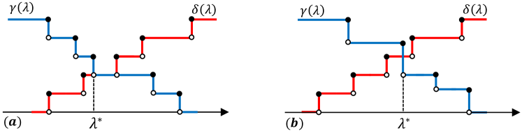
Figure 1. Choice of $\lambda^{*}$ in (4.99). (a) When $m=n$ and all $m+n$ coordinates in $(\boldsymbol{\alpha},\boldsymbol{\beta})$ are distinct, then we can take $\lambda^{*}$ to be a continuity point of both $\delta(\lambda)$ and $\gamma(\lambda)$ such that $\delta(\lambda^{*})=\gamma(\lambda^{*})$. (b) In the general case, we can choose $\lambda^{*}$ to be a discontinuity point of $\gamma(\lambda)$ where the jump of $\gamma$ at $\lambda^{*}$ intersect with $\delta$.

In the remainder of the proof, we will consider the shifted MLE $(\boldsymbol{\alpha}^{*},\boldsymbol{\beta}^{*}):=(\boldsymbol{\alpha}+\lambda^{*}\mathbf{1}_{m},\boldsymbol{\beta}-\lambda^{*}\mathbf{1}_{n})$. We will denote $\boldsymbol{\alpha}^{*}=(\alpha_{1}^{*},\dots,\alpha_{m}^{*})$ and $\boldsymbol{\beta}^{*}=(\beta_{1}^{*},\dots,\beta_{n}^{*})$ and $\delta:=\delta(\lambda^{*})$ and $\gamma:=\gamma(\lambda^{*})$. An important consequence of (4.99) is that

(4.100) $$\delta=w|\{j\,:\,\beta_{j}^{*}=0\}|/n+|\{j\,:\,\beta_{j}^{*}>0\}|/n\quad\textup{for some $w\in[0,1]$}.$$

Fix $\varepsilon>0$ sufficiently small. Note that $\phi(x)\rightarrow-\infty$ as $x\searrow 0$ and $\phi(B-x)\rightarrow\infty$ as $x\searrow 0$. Hence there are constants $c_{1},c_{2}$ (depending on $\varepsilon$) such that

(4.101) $$\phi(c_{1})+\phi(B-\varepsilon)\leq\phi(s-\varepsilon),\qquad\phi(\varepsilon)+\phi(B-c_{2})\geq\phi(t+\varepsilon).$$

Then, for fixed $\varepsilon,c_{1},c_{2}$, we may choose $c_{3},c_{4}$ small enough so that

(4.102) $$\phi(c_{3})+\phi(B-c_{2})\leq\phi(s-\varepsilon),\qquad\phi(c_{1})+\phi(B-c_{4})\geq\phi(t+\varepsilon).$$

We claim that

(4.103) $$\phi(c_{1}) \overset{(a)}{\leq}\alpha_{1}^{*}\leq\alpha_{m}^{*}\overset{(b)}{\leq}\phi(B-c_{2}),\qquad\phi(c_{3})\overset{(c)}{\leq}\beta_{1}^{*}\leq\beta_{n}^{*}\overset{(d)}{\leq}\phi(B-c_{4}).$$

Since $\phi(z_{ij})=\alpha_{i}^{*}+\beta_{j}^{*}$ and $\phi$ is non-decreasing, the assertion follows immediately from this claim. Inequalities (c) and (d) follow easily from assuming (a) and (b). Indeed, suppose (d) is not true while (a) holds. Then

(4.104) $$tm\geq c_{n}=\sum_{i}z_{i,n}=\sum_{i}\psi^{\prime}(\alpha^{*}_{i}+\beta_{n}^{*})\geq m\,\psi^{\prime}(\phi(c_{1})+\phi(B-c_{4}))\geq(t+\varepsilon)m,$$

which is a contradiction. Thus if we show (a) holds, then (d) also holds. Similarly, if (c) is not true while (b) holds, then

(4.105) $$sn\leq\mathbf{r}(i)=\sum_{i}z_{i,1}=\sum_{i}\psi^{\prime}(\alpha^{*}_{i}+\beta_{1}^{*})\leq n\,\psi^{\prime}(\phi(B-c_{2})+\phi(A+c_{3}))\leq(s-\varepsilon)n,$$

which is a contradiction. Therefore, it remains to show (4.103)(a)-(b).

In the remainder of the proof, we will use the following observation: Since $\psi^{\prime}$ is decreasing, and $\alpha_{1}^{*}\leq\dots\leq\alpha_{m}^{*}$ and $\beta_{1}^{*}\leq\dots\leq\beta_{n}^{*}$, for all $i,j$,

(4.106) $$z_{i,n} =\psi^{\prime}(\alpha^{*}_{i}+\beta^{*}_{n})\geq z_{1,n}\geq\psi^{\prime}(\alpha^{*}_{1}+\beta^{*}_{j})=z_{1,j},$$

(4.107) $$z_{m,j} =\psi^{\prime}(\alpha^{*}_{m}+\beta^{*}_{j})\geq z_{m,1}\geq\psi^{\prime}(\alpha^{*}_{i}+\beta^{*}_{1})=z_{i,1}.$$

First we show (4.103)(a). Suppose for contradiction (a) does not hold, i.e., $\alpha^{*}_{1}<\phi(c_{1})$. Then necessarily $\beta^{*}_{n}>\phi(B-\varepsilon)$, since otherwise for all $1\leq j\leq n$,

(4.108) $$z_{1,j}=\psi^{\prime}(\alpha^{*}_{1}+\beta^{*}_{j})\leq\psi^{\prime}(\alpha^{*}_{1}+\beta^{*}_{n})\leq\psi^{\prime}\left(\phi(c_{1})+\phi(B-\varepsilon)\right)\leq\psi^{\prime}(\phi(s-\varepsilon))=s-\varepsilon.$$

So this implies $s\leq r_{1}/m\leq s-\varepsilon$, a contradiction.

Now since $\alpha^{*}_{1}<\phi(c_{1})$ and $\beta^{*}_{n}>\phi(B-\varepsilon)$,

(4.109) $$z_{i,n} =\psi^{\prime}(\alpha^{*}_{i}+\beta^{*}_{n})\geq\psi^{\prime}(\beta^{*}_{n})\geq\psi^{\prime}(\phi(B-\varepsilon))=B-\varepsilon\qquad\textup{if $\alpha^{*}_{i}\geq 0$ },$$

(4.110) $$z_{1,j} =\psi^{\prime}(\alpha^{*}_{1}+\beta^{*}_{j})\leq\psi^{\prime}(\alpha^{*}_{1})\leq\psi^{\prime}(\phi(c_{1}))=c_{1}\qquad\textup{if $\beta^{*}_{j}\leq 0$}.$$

Then using (4.100),

(4.111) $$tm\geq c_{n}=\sum_{i}z_{i,n}=\sum_{i;\alpha^{*}_{i}\geq 0}z_{i,n}+\sum_{i;\alpha^{*}_{i}<0}z_{i,n}\geq m\delta(B-\varepsilon)+(1-\delta)mz_{1,n},$$

(4.112) $$sn\leq r_{1}=\sum_{j}z_{1,j}=\left(\sum_{j;\beta^{*}_{j}<0}z_{1,j}+(1-w)\sum_{j;\beta^{*}_{j}=0}z_{1,j}\right)+\left(w\sum_{j;\beta^{*}_{j}=0}z_{1,j}+\sum_{j;\beta^{*}_{j}>0}z_{1,j}\right)$$

(4.113) $$\hskip 73.69252pt\leq(1-\delta)c_{1}+\delta nz_{1,n}.$$

It follows that

(4.114) $$t\geq\delta(B-\varepsilon)+(1-\delta)z_{1,n},\qquad s\leq(1-\delta)c_{1}+\delta z_{1,n}.$$

Denote $\tau=z_{1,n}$. Using $\delta\in[0,1]$,

(4.115) $$t+\varepsilon\geq\delta B+(1-\delta)\tau,\qquad s-c_{1}\leq\delta\tau.$$

From $\frac{\delta B+\tau}{2}\geq\sqrt{\delta B\tau}$, we get

(4.116) $$\delta B+(1-\delta)\tau\geq 2\sqrt{\delta B\tau}-\delta\tau.$$

For $c>0$, the function $h_{c}(x):=2\sqrt{Bcx}-cx$ is increasing for $x\in[0,B/c]$. So (4.115) gives

(4.117) $$t+\varepsilon\geq\delta B+(1-\delta)\tau\geq h_{1}(\delta\tau)\geq h_{1}\left(s-c_{1}\right)=h_{s-c_{1}}(1).$$

Thus if

(4.118) $$t+\varepsilon<h_{s-c_{1}}(1),$$

then this leads to a contradiction. Note that (4.118) holds for $\varepsilon,c_{1}$ sufficiently small if $t<h_{s}(1)$. The latter condition is $t<2\sqrt{Bs}-s$, or $(s+t)^{2}<4Bs$. Thus we conclude that (4.103)(a) hold.

By an entirely symmetric argument, we can show that if (4.103)(b) holds. We omit the details. ∎

5. Proof of results for typical kernels

We first recall the following standard fact about step function approximation.

Lemma 5.1 (Approximation by stepfunctions in $L^{1}$).

Suppose $|A|,|B|<\infty$ and let $h:[A,B]^{d}\rightarrow\mathbb{R}$ be a measurable function for some integer $d\geq 1$. Then there exists a sequence of stepfunctions $(h_{n})_{n\geq 1}$ such that $\lVert h_{n}-h\rVert_{1}\rightarrow 0$ as $n\rightarrow\infty$.

Typical construction of such stepfunctions in Lemma 5.1 is by block-averaging over diadic partitions. The $L^{1}$ convergence can be shown by applying Lévy’s upward convergence theorem. We omit the details.

Next, we establish the basic properties of the function $G$ in (2.33).

Proposition 5.2.

The function $G$ in (2.33) is well-defined and strictly convex. Furthermore, for any $\delta>0$, $G$ restricted on $\mathcal{W}^{[A_{\delta},B_{\delta}]}$ is lower semi-continuous with respect to the cut distance $\delta_{\square}$.

Proof.

By the assumption on $\mu$, there exists some tilting parameter $\theta_{0}\in\Theta$, for which $\mu_{\theta_{0}}$ is a probability measure. Fix $\theta\in\Theta$. Noting that the KL divergence between two probability distributions is nonnegative,

(5.1) $$D(\mu_{\theta}\|\mu) =\left[(\theta-\theta_{0})\psi^{\prime}(\theta)-\psi(\theta)+\psi(\theta_{0})\right]+\theta_{0}\psi^{\prime}(\theta)-\psi(\theta_{0})$$

(5.2) $$=D(\mu_{\theta}\,\|\,\mu_{\theta_{0}})+\theta_{0}\psi^{\prime}(\theta)-\psi(\theta_{0})$$

(5.3) $$\geq\theta_{0}\psi^{\prime}(\theta)-\psi(\theta_{0}).$$

It follows that for the function $f(x)=D(\mu_{\phi(x)}\|\mu)$ in (2.1), $f(x)\geq\theta_{0}x-\psi(\theta_{0})$. This yields that $G(W)\in(-\infty,\infty]$ for all $W\in\mathcal{W}^{(A,B)}$ since

(5.4) $$G(W)=\int_{[0,1]^{2}}f(W(x,y))\,dxdy\geq\theta_{0}\int_{[0,1]^{2}}W(x,y)\,dxdy-\psi(\theta_{0})>-\infty.$$

For strict convexity, fix $\lambda\in(0,1)$. Since $f$ is strictly convex on $(A,B)$ (see (4.8)), we have $f(\lambda y+(1-\lambda)x)<\lambda f(y)+(1-\lambda)f(x)$ for $x,y\in(A,B)$ and $x\neq y$. It follows that $G(\lambda W^{\prime}+(1-\lambda)W)<\lambda G(W^{\prime})+(1-\lambda)G(W)$ for $W,W^{\prime}\in\mathcal{W}^{(A,B)}$ with $W\neq W^{\prime}$ almost surely.

Next, we consider $G$ restricted on $\mathcal{W}^{[A_{\delta},B_{\delta}]}$. To show lower semi-continuity, let $W_{k}$ be a sequence of functions in $\mathcal{W}^{[A_{\delta},B_{\delta}]}$ converging to $W\in\mathcal{W}^{[A_{\delta},B_{\delta}]}$ in $\delta_{\square}$-metric. We wish to show that

(5.5) $$\mathop{\rm lim\,inf}\limits_{k\rightarrow\infty}\,G(W_{k})\geq G(W).$$

Noting that $G(W)=G(W(\xi(\cdot),\eta(\cdot)))$ for every measure-preserving transformations $\xi,\eta$ on $[0,1]$, without loss of generality we can assume $\lVert W_{k}-W\rVert_{\square}\rightarrow 0$ as $k\rightarrow\infty$.

Define $W^{L}$ to be the $L\times L$ block-ageraging of $W$ for every $W\in\mathcal{W}$ and $L>0$. By convexity of $G$ and Jensen’s inequality, $G(W_{k})\geq G(W_{k}^{L})$. For fixed $L$, $G(W_{k}^{L})\rightarrow G(W^{L})$ using the continuity of $G$ on $L\times L$ stepfunctions. It follows that

(5.6) $$\mathop{\rm lim\,inf}\limits_{k\rightarrow\infty}\,G(W_{k})\geq\mathop{\rm lim\,inf}\limits_{L\rightarrow\infty}\,\mathop{\rm lim\,inf}\limits_{k\rightarrow\infty}\,G(W_{k}^{L})=\mathop{\rm lim\,inf}\limits_{L\rightarrow\infty}\,G(W^{L}).$$

Hence it suffices to show that

(5.7) $$\mathop{\rm lim\,inf}\limits_{L\rightarrow\infty}\,G(W^{L})\geq G(W).$$

To this end, let $U,V$ be independent uniform $[0,1]$ variables. Then $W^{L}(U,V)$ converges to $W(U,V)$ in probability. For every integrable function $W^{\prime}:[0,1]\rightarrow\mathbb{R}$, we have $G(W^{\prime})=\mathbb{E}[f(W^{\prime}(U,V))]$. Then noting that $f$ is continuous and the range of $f\circ W^{L}$ is in $[A_{\delta},B_{\delta}]$ for all $L\geq 1$, we get

(5.8) $$\lim_{L\rightarrow\infty}\,G(W^{L})=\lim_{L\rightarrow\infty}\,\mathbb{E}[f(W^{L}(U,V))]=\mathbb{E}[f(W(U,V))]=G(W),$$

where the equality in the middle follows from the bounded convergence theorem noting that $f\circ W$ is bounded for $W$ taking values from $[A_{\delta},B_{\delta}]$. ∎

Proposition 5.3.

Let $(\mathbf{r},\mathbf{c})$ be an $m\times n$ margin with typical table $Z^{\mathbf{r},\mathbf{c}}\in(A,B)^{m\times n}$. Then $W_{Z^{\mathbf{r},\mathbf{c}}}$ is the unique typical kernel for the continuum margin $(\bar{\mathbf{r}},\bar{\mathbf{c}})$.

Proof.

Denote $W^{*}:=W_{Z^{\mathbf{r},\mathbf{c}}}$. Let $I_{1}\sqcup\dots\sqcup I_{m}=[0,1]$ and $J_{1}\sqcup\dots\sqcup J_{n}=[0,1]$ be the interval partitions for $\bar{\mathbf{r}}$ and $\bar{\mathbf{c}}$, respectively. Fix any kernel $W\in\mathcal{W}_{\overline{\mathbf{r}},\overline{\mathbf{c}}}^{(A,B)}$. Let $\overline{W}$ denote the block-averaged version of $W$, which takes the contant value $\frac{1}{|I_{i}|\cdot|J_{j}|}\int_{I_{i}\times J_{j}}W(x,y)\,dx\,dy$ on the rectanble $I_{i}\times J_{j}$ for all $i,j$. Note that $\overline{W}\in\mathcal{W}_{\overline{\mathbf{r}},\overline{\mathbf{c}}}^{(A,B)}$. Since $G$ is concave, by Jensen’s inequality, $G(W)\leq G(\overline{W})$. Also clearly $\overline{W^{*}}=W^{*}$ and $W^{*}\in\mathcal{W}_{\overline{\mathbf{r}},\overline{\mathbf{c}}}^{(A,B)}$. It follows that

(5.9) $$\inf_{W\in\mathcal{W}_{\mathbf{r},\mathbf{c}}^{(A,B)}}G(W)=\inf_{W\in\mathcal{W}_{\mathbf{r},\mathbf{c}}^{(A,B)}}G(\overline{W}).$$

That is, the function $G$ is maximized over step kernels. Maximizing $G$ over the $m\times n$ step kernels with continuum margin $(\bar{\mathbf{r}},\bar{\mathbf{c}})$ is exactly the typical table problem that $Z^{\mathbf{r},\mathbf{c}}$ solves for the discrete margin $(\mathbf{r},\mathbf{c})$. This is enough to conclude. ∎

Next, we prove the characterization of typical kernels and tame margins stated in Lemma 2.14.

Proof of Lemma 2.14.

We first show (a). By the hypothesis of part (a), the typical table $W^{\mathbf{r},\mathbf{c}}$ exists and it is $\delta$-tame. Let $U(\cdot,\cdot)$ be a measurable function from $[0,1]^{2}$ to $[-1,1]$ which satisfies $U(\cdot,\bullet)=U(\bullet,\cdot)\stackrel{{\scriptstyle a.s.}}{{=}}0.$ Then the function $\widetilde{W}^{(\lambda)}:=W^{\mathbf{r},\mathbf{c}}+\lambda U\in\mathcal{W}_{\mathbf{r},\mathbf{c}}$ for all $\lambda\in(-\delta,\delta)$. Since $W^{\mathbf{r},\mathbf{c}}$ is the typical table, the function $\lambda\mapsto G(\widetilde{W}^{(\lambda)})$ is uniquely maximized on $(-\delta,\delta)$ at $\lambda=0$, which gives

$$0=\frac{\partial}{\partial\lambda}G(\widetilde{W}^{(\lambda)})\Big{|}_{\lambda=0}=\int_{[0,1]^{2}}\phi\left(W^{\mathbf{r},\mathbf{c}}(x,y)\right)U(x,y)dxdy.$$

Since this holds for all bounded measurable $U$ which integrates to $0$ along both marginals, it follows that there exists functions $\boldsymbol{\alpha},\boldsymbol{\beta}:[0,1]\mapsto\mathbb{R}$ such that

$$\phi\left(W^{\mathbf{r},\mathbf{c}}(x,y)\right)\stackrel{{\scriptstyle a.s.}}{{=}}\boldsymbol{\alpha}(x)+\boldsymbol{\beta}(y),\text{ which implies }W^{\mathbf{r},\mathbf{c}}(x,y)\stackrel{{\scriptstyle a.s.}}{{=}}\psi^{\prime}(\boldsymbol{\alpha}(x)+\boldsymbol{\beta}(y)).$$

Finally, the fact that $W^{\mathbf{r},\mathbf{c}}$ is $\delta$-tame implies $\phi(A_{\delta})\stackrel{{\scriptstyle a.s.}}{{\leq}}\boldsymbol{\alpha}(x)+\boldsymbol{\beta}(y)\stackrel{{\scriptstyle a.s.}}{{\leq}}\phi(B_{\delta})$. Since changing $(\boldsymbol{\alpha},\boldsymbol{\beta})$ to $(\boldsymbol{\alpha}+\eta,\boldsymbol{\beta}-\eta)$ has no impact on $W^{\mathbf{r},\mathbf{c}}$ for any $\eta\in\mathbb{R}$, we can assume without loss of generality that $\int_{[0,1]}\boldsymbol{\alpha}(x)dx=0$. This, along with the previous display implies

$$\phi(A_{\delta})\stackrel{{\scriptstyle a.s.}}{{\leq}}\boldsymbol{\beta}(y)\stackrel{{\scriptstyle a.s.}}{{\leq}}\phi(B_{\delta}),$$

which in turn implies

$$\phi(A_{\delta})-\phi(B_{\delta})\stackrel{{\scriptstyle a.s}}{{\leq}}\boldsymbol{\alpha}(x)\stackrel{{\scriptstyle a.s}}{{\leq}}\phi(B_{\delta})-\phi(A_{\delta}).$$

The desired conclusion of part (a) follows.

Next, we show (b). Let $\widetilde{W}\in\mathcal{W}_{\mathbf{r},\mathbf{c}}$ be arbitrary. It suffices to show that $G(W^{*})\geq G(\widetilde{W})$. Since $G$ is strictly convex, it suffices to show that the function $\lambda\mapsto G\left((1-\lambda)W^{*}+\lambda\widetilde{W}\right)$ on $[0,1]$ has a derivative which vanishes at $\lambda=0$. This is equivalent to checking

$$\int_{[0,1]^{2}}\phi\left(W^{*}(x,y)\right)U(x,y)dxdy=0,\text{ where }U=W^{*}-\widetilde{W}.$$

But this follows on noting that $\phi\left(W^{*}(x,y)\right)=\boldsymbol{\alpha}(x)+\boldsymbol{\beta}(y)$, and $U(\cdot,\bullet)=U(\bullet,\cdot)\stackrel{{\scriptstyle a.s.}}{{=}}0$. ∎

We now prove Lipschitz continuity of typical kernels and dual variables stated in Theorem 2.15. Our approach is to extend the discrete analog (Thm. 2.6) to the continuous case by discretizing the dual variables and passing to the limit. The key ingredient for these continuous extensions is Lemma 2.14, which we have established above.

Proof of Theorem 2.15.

We will first show (2.38) by pushing the discrete result in Lemma 2.14 to continuum limit by block averaging. Fix an integer $L\geq 1$. Then by Lemma 2.14, there exists bounded and measurable functions $\boldsymbol{\alpha},\boldsymbol{\beta},\boldsymbol{\alpha}^{\prime},\boldsymbol{\beta}^{\prime}:[0,1]\rightarrow[-2C_{\delta},2C_{\delta}]$ such that

(5.10) $$W^{\mathbf{r},\mathbf{c}}(x,y)=\psi^{\prime}(\boldsymbol{\alpha}(x)+\boldsymbol{\beta}(y))\quad\textup{and}\quad W^{\mathbf{r}^{\prime},\mathbf{c}^{\prime}}(x,y)=\psi^{\prime}(\boldsymbol{\alpha}^{\prime}(x)+\boldsymbol{\beta}^{\prime}(y)),$$

where $W^{\mathbf{r},\mathbf{c}},W^{\mathbf{r}^{\prime},\mathbf{c}^{\prime}}\in\mathcal{W}^{[A_{\delta},B_{\delta}]}$. In particular,

(5.11) $$\mathbf{r}(x) =\int_{0}^{1}\psi^{\prime}(\boldsymbol{\alpha}(x)+\boldsymbol{\beta}(y))\,dy,\quad\mathbf{c}(y)=\int_{0}^{1}\psi^{\prime}(\boldsymbol{\alpha}(x)+\boldsymbol{\beta}(y))\,dx,$$

(5.12) $$\mathbf{r}^{\prime}(x) =\int_{0}^{1}\psi^{\prime}(\boldsymbol{\alpha}^{\prime}(x)+\boldsymbol{\beta}^{\prime}(y))\,dy,\quad\mathbf{c}^{\prime}(y)=\int_{0}^{1}\psi^{\prime}(\boldsymbol{\alpha}^{\prime}(x)+\boldsymbol{\beta}^{\prime}(y))\,dx.$$

For each function $h:[0,1]\rightarrow\mathbb{R}$ and an integer $L\geq 1$, let $h_{L}$ denote the block average of $h$ over intervals $[(i-1)2^{-L},i2^{-L})$ for $i=1,\dots,2^{L}$. By Lemma 5.1, there exists $\varepsilon=\varepsilon(L)>0$ such that

(5.13) $$\lVert\boldsymbol{\alpha}-\boldsymbol{\alpha}_{L}\rVert_{1}+\lVert\boldsymbol{\beta}-\boldsymbol{\beta}_{L}\rVert_{1}+\lVert\boldsymbol{\alpha}^{\prime}-\boldsymbol{\alpha}^{\prime}_{L}\rVert_{1}+\lVert\boldsymbol{\beta}^{\prime}-\boldsymbol{\beta}^{\prime}_{L}\rVert_{1}\leq\varepsilon(L)\rightarrow 0\quad\textup{as $L\rightarrow\infty$.}$$

Now define block margin $(\mathbf{r}_{L},\mathbf{c}_{L})$ by

(5.14) $$\mathbf{r}_{L}(x)=\int_{0}^{1}\psi^{\prime}(\boldsymbol{\alpha}_{L}(x)+\boldsymbol{\beta}_{L}(y))\,dy,\quad\mathbf{c}_{L}(y)=\int_{0}^{1}\psi^{\prime}(\boldsymbol{\alpha}_{L}(x)+\boldsymbol{\beta}_{L}(y))\,dx.$$

Namely, the block margin $(\mathbf{r}_{L},\mathbf{c}_{L})$ is obtained by taking block-average of the dual variable $(\boldsymbol{\alpha},\boldsymbol{\beta})$. Further, note that from (5.10),

(5.15) $$\phi(A_{\delta})\leq\boldsymbol{\alpha}_{L}(x)+\boldsymbol{\beta}_{L}(y)\leq\phi(B_{\delta})\quad\textup{and}\quad\phi(A_{\delta})\leq\boldsymbol{\alpha}^{\prime}_{L}(x)+\boldsymbol{\beta}^{\prime}_{L}(y)\leq\phi(B_{\delta}).$$

Hence $(\mathbf{r}_{L},\mathbf{c}_{L})$ and $(\mathbf{r}^{\prime}_{L},\mathbf{c}^{\prime}_{L})$ are both $\delta$-tame margins for all $L\geq 1$.

Denote

(5.16) $$D_{\delta}:=\sup_{\phi(A_{\delta})\leq w\leq\phi(B_{\delta})}\psi^{\prime\prime}(w)>0.$$

Note that

(5.17) $$\lVert\mathbf{r}-\mathbf{r}_{L}\rVert_{1}+\lVert\mathbf{c}-\mathbf{c}_{L}\rVert_{1} \leq 2\int_{[0,1]^{2}}\left|\psi^{\prime}(\boldsymbol{\alpha}_{L}(x)+\boldsymbol{\beta}_{L}(y))-\psi^{\prime}(\boldsymbol{\alpha}(x)+\boldsymbol{\beta}(y))\right|\,dy\,dx$$

(5.18) $$\leq D_{\delta}\int_{[0,1]^{2}}|\boldsymbol{\alpha}_{L}(x)-\boldsymbol{\alpha}(x)|+|\boldsymbol{\beta}_{L}(y)-\boldsymbol{\beta}(y)|\,dy\,dx$$

(5.19) $$\leq 2D_{\delta}\varepsilon(L).$$

By a similar argument,

(5.20) $$\lVert\mathbf{r}^{\prime}-\mathbf{r}^{\prime}_{L}\rVert_{1}+\lVert\mathbf{c}^{\prime}-\mathbf{c}^{\prime}_{L}\rVert_{1}\leq 2D_{\delta}\varepsilon(L).$$

Then by a triangle inequality,

(5.21) $$\lVert W^{\mathbf{r},\mathbf{c}}-W^{\mathbf{r}^{\prime},\mathbf{c}^{\prime}}\rVert_{2}\leq\lVert W^{\mathbf{r},\mathbf{c}}-W^{\mathbf{r}_{L},\mathbf{c}_{L}}\rVert_{2}+\lVert W^{\mathbf{r}^{\prime},\mathbf{c}^{\prime}}-W^{\mathbf{r}^{\prime}_{L},\mathbf{c}^{\prime}_{L}}\rVert_{2}+\lVert W^{\mathbf{r}_{L},\mathbf{c}_{L}}-W^{\mathbf{r}^{\prime}_{L},\mathbf{c}^{\prime}_{L}}\rVert_{2}.$$

In order to bound the last term, we can apply Theorem 2.6 since both the margins and the typical kernels are stepfunctions on the intervals $[(i-1)2^{-L},i2^{-L})$, $i=1,\dots,2^{L}$ and rectangles form by them, respectively. Thus by Theorem 2.6 and inequalities (5.17) and (5.20),

(5.22) $$\lVert W^{\mathbf{r}_{L},\mathbf{c}_{L}}-W^{\mathbf{r}^{\prime}_{L},\mathbf{c}^{\prime}_{L}}\rVert_{2}^{2} \leq 2C_{\delta}D_{\delta}\lVert(\mathbf{r}_{L},\mathbf{c}_{L})-(\mathbf{r}^{\prime}_{L},\mathbf{c}^{\prime}_{L})\rVert_{1}\leq 2C_{\delta}D_{\delta}\left(4D_{\delta}\varepsilon+\lVert(\mathbf{r},\mathbf{c})-(\mathbf{r}^{\prime},\mathbf{c}^{\prime})\rVert_{1}\right).$$

The first two terms on the right-hand side of (5.21) vanishes as $L,L^{\prime}\rightarrow\infty$ by Proposition 2.13. This shows (2.38).

Next, we show the Lipschitz continuity of MLEs as stated in (2.39). By mean value theorem and (2.2), $\phi$ restricted on $[A_{\delta},B_{\delta}]$ is $L$-Lipschitz continuous for

(5.23) $$L=\sup_{A_{\delta}\leq t\leq B_{\delta}}\frac{1}{\psi^{\prime\prime}(\phi(t))}=\frac{1}{\inf_{\phi(A_{\delta})\leq w\leq\phi(B_{\delta})}\psi^{\prime\prime}(w)}.$$

Define a kernel $V(x,y):=\boldsymbol{\alpha}(x)+\boldsymbol{\beta}(y)=\phi(W^{\mathbf{r},\mathbf{c}}(x,y))$ for $x,y\in[0,1]$ and similarly define $V^{\prime}$ using $(\boldsymbol{\alpha}^{\prime},\boldsymbol{\beta}^{\prime})$. Then by a simple computation using the fact that $\int_{0}^{1}\boldsymbol{\alpha}(x)\,dx=\int_{0}^{1}\boldsymbol{\alpha}^{\prime}(x)\,dx=0$, we have

(5.24) $$\lVert\boldsymbol{\alpha}-\boldsymbol{\alpha}^{\prime}\rVert_{2}^{2}+\lVert\boldsymbol{\beta}-\boldsymbol{\beta}^{\prime}\rVert_{2}^{2}=\lVert V-V^{\prime}\rVert_{2}^{2}\leq L\lVert W^{\mathbf{r},\mathbf{c}}-W^{\mathbf{r}^{\prime},\mathbf{c}^{\prime}}\rVert_{2}^{2}.$$

Then (2.39) follows from the above and (2.38). ∎

Lastly in this section, we prove Proposition 2.13.

Proof of Proposition 2.13..

Let $Z_{k}$ denote the typical table for the $(m_{k}\times n_{k})$ $\delta$-tame margin $(\mathbf{r}_{m_{k}},\mathbf{c}_{n_{k}})$. By Proposition 5.3, $W_{k}:=W_{Z_{k}}$ is the typical kernel for the corresponding continuum step margin $(\bar{\mathbf{r}}_{m_{k}},\bar{\mathbf{c}}_{n_{k}})$ (see (1.16)). By Theorem 2.15, $W_{k}$ converges to some kernel $W^{*}$ in $L^{2}$ as $k\rightarrow\infty$. Since $W_{k}\in\mathcal{W}^{[A_{\delta},B_{\delta}]}$, it follows that $W^{*}\in\mathcal{W}^{[A_{\delta},B_{\delta}]}$. It is easy to see that $W^{*}$ has continuum margin $(\mathbf{r},\mathbf{c})$.

By Lemma 2.14, there exists a constant $C=C_{\delta}>0$ such that for each $k\geq 1$, there exists bounded measurable functions $\boldsymbol{\alpha}_{k},\boldsymbol{\beta}_{k}:[0,1]\rightarrow[-C,C]$ for which

(5.25) $$W_{k}(x,y)\overset{a.s.}{=}\psi^{\prime}(\boldsymbol{\alpha}_{k}(x)+\boldsymbol{\beta}_{k}(y)).$$

Without loss of generality, we may assume $\int_{0}^{1}\boldsymbol{\alpha}_{k}(x)\,dx=0$ for all $k\geq 1$. Then by (2.39) in Theorem 2.15, we have that $\boldsymbol{\alpha}_{k}\rightarrow\boldsymbol{\alpha}^{*}$ and $\boldsymbol{\beta}_{k}\rightarrow\boldsymbol{\beta}^{*}$ in $L^{2}$ for some bounded measurable functions $\boldsymbol{\alpha}^{*},\boldsymbol{\beta}^{*}:[0,1]\rightarrow[-C,C]$. Note that $\int_{0}^{1}\boldsymbol{\alpha}^{*}(x)\,dx=0$.

Now define a kernel $W^{*}(x,y)=\psi^{\prime}(\boldsymbol{\alpha}^{*}(x)+\boldsymbol{\beta}^{*}(x))$. By mean value theorem, $\psi^{\prime}$ restricted on $[\phi(A_{\delta}),\phi(B_{\delta})]$ is $L$-Lipschitz continuous for some constant $L=L(\delta)>0$. Hence

(5.26) $$\lVert W_{k}-W^{*}\rVert_{2}^{2}\leq L(\lVert\boldsymbol{\alpha}_{k}-\boldsymbol{\alpha}^{*}\rVert_{2}^{2}+\lVert\boldsymbol{\beta}_{k}-\boldsymbol{\beta}^{*}\rVert_{2}^{2}).$$

It follows that $W_{k}\rightarrow W^{*}$ in $L^{2}$. Since $W_{k}\in\mathcal{W}_{\bar{\mathbf{r}}_{k},\bar{\mathbf{c}}_{k}}^{[A_{\delta},B_{\delta}]}$ and $(\bar{\mathbf{r}}_{k},\bar{\mathbf{c}}_{k})\rightarrow(\mathbf{r},\mathbf{c})$ in $L^{1}$, this yields $W^{*}\in\mathcal{W}_{\mathbf{r},\mathbf{c}}^{[A_{\delta},B_{\delta}]}$. By definition of $W^{*}$ and Lemma 2.14, we deduce that $W^{*}$ is the unique typical kernel for margin $(\mathbf{r},\mathbf{c})$. Since $W^{*}$ takes values from $[A_{\delta},B_{\delta}]$, we conclude that $(\mathbf{r},\mathbf{c})$ is $\delta$-tame. ∎

6. Proof of Theorems 1.5, 1.7, and Corollary 1.8.

Proposition 6.1.

Let $A\in\mathbb{R}^{m\times n}$ and let $W_{A}$ denote the corresponding kernel. Then

(6.1) $$mn\lVert W_{A}\rVert_{\square}=\sup_{\mathbf{x}\in\{0,1\}^{m},\,\mathbf{y}\in\{0,1\}^{n}}|\mathbf{x}^{T}A\mathbf{y}|.$$

Proof.

Write $I_{i}=((i-1)/m,i/m]$ for $i=1,\dots,m$ and $J_{j}=((j-1)/n,j/n]$ for $j=1,\dots,n$. We first claim that the supremum in $\lVert W_{A}\rVert_{\square}$ is attained over a measurable rectangle $S\times T\subseteq[0,1]^{2}$, where $S$ is the disjoint union of some of the intervals $I_{i}$s and $T$ is the disjoint union of some of the intervals $J_{j}$s. This claim will show the first equality in the assertion, and the second equality there follows from the definition of the cut norm of a matrix.

It remains to show the claim. Recall that $W_{A}$ takes the constant value $A_{ij}$ over the rectangle $I_{i}\times J_{j}$. Then

(6.2) $$\int_{S\times T}W_{A}\,dx\,dy =\sum_{i}|S\cap I_{i}|\left(\sum_{j}|T\cap J_{j}|A_{ij}\right).$$

If the quantity in the parenthesis on the right-hand side is nonnegative, then replacing $S\cap I_{i}$ with $I_{i}$ can only increase the total value; otherwise, replace $S\cap I_{i}$ with $\emptyset$. In this way, we find a new set $\bar{S}$ that is the disjoint union of some of $I_{i}$’s such that

(6.3) $$\int_{S\times T}W_{A}\,dx\,dy\leq\int_{\bar{S}\times T}W_{A}\,dx\,dy.$$

Similarly, we can find a disjoint union $\bar{T}$ of some of $J_{j}$’s such that

(6.4) $$\int_{S\times T}W_{A}\,dx\,dy\leq\int_{\bar{S}\times T}W_{A}\,dx\,dy\leq\int_{\bar{S}\times\bar{T}}W_{A}\,dx\,dy.$$

Repeating the same argument with $-W_{A}$, we can deduce the claim. ∎

The main ingredient for the proof of Theorem 1.5, we need is the following Hoeffding’s inequality for the maximum likelihood $(\boldsymbol{\alpha},\boldsymbol{\beta})$-model for a $\delta$-tame margin.

Lemma 6.2 (Hoeffding’s inequality for the $(\boldsymbol{\alpha},\boldsymbol{\beta})$-model).

Let $(\mathbf{r},\mathbf{c})$ be an $m\times n$ $\delta$-tame margin and $Y\sim\boldsymbol{\mu}_{\boldsymbol{\alpha},\boldsymbol{\beta}}$, where $(\boldsymbol{\alpha},\boldsymbol{\beta})$ is an MLE for the margin $(\mathbf{r},\mathbf{c})$. Define positive constants

(6.5) $$L_{-}:=\min\left\{\phi(A_{\delta})-\phi(A_{\delta/2}),\,\phi(B_{\delta/2})-\phi(B_{\delta})\right\},\quad L^{+}:=\max\left\{\psi^{\prime\prime}(\phi(A_{\delta/2})),\,\psi^{\prime\prime}(\phi(B_{\delta/2}))\right\}.$$

Denote $\bar{Y}=Y-\mathbb{E}[Y]$. For each $s\in[0,L_{-}L^{+}]$, we have

(6.6) $$\mathbb{P}\left(\lVert W_{\bar{Y}}\rVert_{\square}\geq s\right) \leq 2^{m+n+1}\exp\left(-\frac{s^{2}mn}{2L^{+}}\right),$$

(6.7) $$\mathbb{P}(Y\in\mathcal{T}_{smn}(\mathbf{r},\mathbf{c})) \geq 1-2^{m+n+1}\exp\left(-\frac{s^{2}mn}{2L^{+}}\right).$$

Furthermore, for each $t>0$ denote $\bar{t}=t\land\tilde{L}$. Then for each $\mathbf{x}\in[0,1]^{m}$ and $\mathbf{y}\in[0,1]^{n}$,

(6.8) $$\mathbb{P}\left(\left|\mathbf{x}^{T}\bar{Y}\mathbf{y}\right|\geq t\lVert\mathbf{x}\rVert^{2}\lVert\mathbf{y}\rVert^{2}\right)\leq 2\exp\left(-\lVert\mathbf{x}\rVert^{2}\lVert\mathbf{y}\rVert^{2}\frac{t(t\land\tilde{L})}{2L^{+}}\right).$$

Proof.

We will first show (6.8). By using a union bound, we only need to show

(6.9) $$\mathbb{P}\left(\mathbf{x}^{T}\bar{Y}\mathbf{y}\geq t\lVert\mathbf{x}\rVert^{2}\lVert\mathbf{y}\rVert^{2}\right)\leq\exp\left(-\lVert\mathbf{x}\rVert^{2}\lVert\mathbf{y}\rVert^{2}\frac{t(t\land\tilde{L})}{2L^{+}}\right).$$

First note that if $X\sim\mu_{\theta}$, then

(6.10) $$\mathbb{E}[\exp(s(X-\mathbb{E}[X]))]=\exp(\psi(s+\theta)-\psi(\theta)-s\psi^{\prime}(\theta)).$$

Write $t^{\prime}:=t\lVert\mathbf{x}\rVert^{2}\lVert\mathbf{y}\rVert^{2}$ and $s^{\prime}_{ij}=s\,\mathbf{x}(i)\mathbf{y}(j)$. For each $s\geq 0$, we have

(6.11) $$\mathbb{P}\left(\mathbf{x}^{T}\bar{Y}\mathbf{y}\geq t^{\prime}\right) =\mathbb{P}\left(\exp\left(s\left(\sum_{i,j}\mathbf{x}(i)\mathbf{y}(j)\left(Y_{ij}-\mathbb{E}[Y_{ij}]\right)\right)\right)\geq e^{st^{\prime}}\right)$$

(6.12) $$\leq\exp\left(-st^{\prime}\right)\mathbb{E}\left[\exp\left(s\left(\sum_{i,j}\mathbf{x}(i)\mathbf{y}(j)\left(Y_{ij}-\mathbb{E}[Y_{ij}]\right)\right)\right)\right]$$

(6.13) $$=\exp\left(-st^{\prime}\right)\prod_{i,j}\mathbb{E}\left[\exp\left(s^{\prime}_{ij}\,\left(Y_{ij}-\mathbb{E}[Y_{ij}]\right)\right)\right]$$

(6.14) $$=\exp\left(-st^{\prime}+\sum_{i,j}\psi(s^{\prime}_{ij}+\theta_{ij})-\psi(\theta_{ij})-s^{\prime}_{ij}\psi^{\prime}(\theta_{ij})\right).$$

Denote $\varphi(s):=\psi(s+\theta)-\psi(\theta)-s\psi^{\prime}(\theta)$. Then

(6.15) $$f^{\prime}(s)=\psi^{\prime}(s+\theta)-\psi^{\prime}(\theta),\quad f^{\prime}(0)=0,\quad f^{\prime\prime}(s)=\psi^{\prime\prime}(s+\theta)\geq 0.$$

Hence $f$ is concave and is minimized at $0$. Let $Z=(z_{ij})$ denote the typical table for $(\mathbf{r},\mathbf{c})$. Since $(\mathbf{r},\mathbf{c})$ is $\delta$-tame, by Lemma 2.5, $\mathbb{E}[Y]=Z\in[A_{\delta},B_{\delta}]^{m\times n}$. So we have

(6.16) $$\phi(A_{\delta/2})\leq s+\phi(z_{ij})\leq\phi(B_{\delta/2})$$

whenever $|s|\leq L_{-}$. Hence

(6.17) $$\sup_{|s|\leq L_{-}}|\varphi^{\prime\prime}(s)|\leq L^{+}.$$

Hence by Taylor’s theorem,

(6.18) $$\varphi(s)\leq\varphi(0)+\varphi^{\prime}(0)s+\frac{L^{+}}{2}s^{2}=\frac{L^{+}}{2}s^{2}\qquad\textup{for all $s\in[0,L_{-}]$}.$$

Applying the above bound for $\theta=\phi(\mathbb{E}[Y_{ij}])$ and $s=s^{\prime}_{ij}$ all $i,j$, from the previous inequality we get

(6.19) $$\mathbb{P}\left(\mathbf{x}^{T}\bar{Y}\mathbf{y}\geq t\lVert\mathbf{x}\rVert^{2}\lVert\mathbf{y}\rVert^{2}\right)\leq\exp\left(-\lVert\mathbf{x}\rVert^{2}\lVert\mathbf{y}\rVert^{2}\left(st-\frac{L^{+}}{2}s^{2}\right)\right)\quad\textup{for all $s\in[0,L_{-}]$},$$

where we have also used $\sum_{i,j}\mathbf{x}(i)^{2}\mathbf{y}(j)^{2}=\lVert\mathbf{x}\rVert^{2}\lVert\mathbf{y}\rVert^{2}$. In order to optimize the above bound, denoting $\bar{t}=t\land L_{-}L^{+}$, write

(6.20) $$st-\frac{L^{+}}{2}s^{2} =s(t-\bar{t})+\left(s\bar{t}-\frac{L^{+}}{2}s^{2}\right).$$

The quadratic function in $s$ in the second term of the right-hand side above is minimized at $s=\bar{t}/L^{+}\in[-L_{-},L_{-}]$ with minimum value $\bar{t}^{2}/2L^{+}$. For this choice of $s$, and noting $t\geq\bar{t}$, the above is at least $\frac{t\bar{t}}{2L^{+}}$. Hence we deduce (6.9) from (6.19). This shows (6.9).

Second, note that by substituting $t=s\frac{mn}{\lVert\mathbf{x}\rVert^{2}\rVert\mathbf{y}\rVert^{2}}$ for $s\in[0,\tilde{L}]$ in (6.8), we get

(6.21) $$\mathbb{P}\left(\left|\mathbf{x}^{T}\bar{Y}\mathbf{y}\right|\geq smn\right) \leq 2\exp\left(-\frac{smn}{2L^{+}}\left(\frac{smn}{\lVert\mathbf{x}\rVert^{2}\rVert\mathbf{y}\rVert^{2}}\land\tilde{L}\right)\right)\leq 2\exp\left(-\frac{s^{2}mn}{2L^{+}}\right),$$

where the last inequality uses $\lVert\mathbf{x}\rVert^{2}\leq m$ and $\lVert\mathbf{y}\rVert^{2}\leq n$.

Now we deduce (6.6). Indeed, using Proposition 6.1 and union bound, for each $s\in[0,L_{-}]$,

(6.22) $$\mathbb{P}\left(\lVert W_{\bar{Y}}\rVert_{\square}\geq s\right)=\mathbb{P}\left(\lVert\bar{Y}\rVert_{\square}\geq smn\right) =\mathbb{P}\left(\max_{\mathbf{x}\in\{0,1\}^{m}\,\mathbf{y}\in\{0,1\}^{n}}|\mathbf{x}^{T}\bar{Y}\mathbf{y}|\geq smn\right)$$

(6.23) $$\leq\sum_{\mathbf{x}\in\{0,1\}^{m}\,\mathbf{y}\in\{0,1\}^{n}}\mathbb{P}\left(|\mathbf{x}^{T}\bar{Y}\mathbf{y}|\geq smn\right)\leq 2^{m+n+1}\exp\left(-\frac{s^{2}mn}{2L^{+}}\right),$$

where the last inequality uses (6.21).

Lastly, we can deduce (6.7) similarly as before. Note that

(6.24) $$\lVert r(\bar{Y})\rVert_{1} =\lVert r(\bar{Y})^{+}\rVert_{1}+\lVert r(\bar{Y})^{-}\rVert_{1}\leq 2\max_{\mathbf{x}\in\{0,1\}^{m}}|\mathbf{x}^{T}\bar{Y}\mathbf{1}_{n}|\leq 2\max_{\mathbf{x}\in\{0,1\}^{m},\mathbf{y}\in\{0,1\}^{n}}|\mathbf{x}^{T}\bar{Y}\mathbf{y}|.$$

The same upper bound holds for $\lVert c(\bar{Y})\rVert_{1}$. Thus, proceeding as before,

(6.25) $$\mathbb{P}(Y\notin\mathcal{T}_{smn}(\mathbf{r},\mathbf{c})) =\mathbb{P}\left(\min\left\{\lVert r(Y)-\mathbf{r}\rVert_{1},\,\lVert c(Y)-\mathbf{c}\rVert_{1}\right\}\geq smn\right)$$

(6.26) $$\leq\mathbb{P}\left(\max_{\mathbf{x}\in\{0,1\}^{m},\mathbf{y}\in\{0,1\}^{n}}|\mathbf{x}^{T}\bar{Y}\mathbf{y}|\geq smn/2\right)\leq 2^{m+n+1}\exp\left(-\frac{s^{2}mn}{2L^{+}}\right).$$

This completes the proof. ∎

Now we are ready to prove Theorems 1.5 and 1.7.

Proof of Theorem 1.5.

Part (i) immediately follows from Lemma 2.5. Part (iii) is a simple consequence of part (ii) and (6.7) in Lemma 6.2. Below we will prove part (ii).

Let $Z=(z_{ij})$ be the typical table for $(\mathbf{r},\mathbf{c})$ and let $(\boldsymbol{\alpha},\boldsymbol{\beta})$ denote a standard MLE for $(\mathbf{r},\mathbf{c})$ as in Lemma 2.5. Note that $\lVert(\boldsymbol{\alpha},\boldsymbol{\beta})\rVert_{\infty}\leq C$ where $C:=2\max\{|\phi(A_{\delta})|,\,|\phi(B_{\delta})|\}$.

Recall that the log-likelihood of observing $\mathbf{x}=(x_{ij})$ under $Y\sim\boldsymbol{\mu}_{\boldsymbol{\alpha},\boldsymbol{\beta}}$ is

(6.27) $$g^{r(\mathbf{x}),c(\mathbf{x})}(\boldsymbol{\alpha},\boldsymbol{\beta})+\log\prod_{i,j}\mu(dx_{ij}).$$

Note that for each $\mathbf{x}\in\mathcal{T}_{\rho}(\mathbf{r},\mathbf{c})$,

(6.28) $$|g^{r(\mathbf{x}),c(\mathbf{x})}(\boldsymbol{\alpha},\boldsymbol{\beta})-g^{\mathbf{r},\mathbf{c}}(\boldsymbol{\alpha},\boldsymbol{\beta})| \leq\lVert\boldsymbol{\alpha}\rVert_{\infty}\lVert r(\mathbf{x})-\mathbf{r}\rVert_{1}+\lVert\boldsymbol{\beta}\rVert_{\infty}\lVert c(\mathbf{x})-\mathbf{c}\rVert_{1}\leq C\rho.$$

Hence

(6.29) $$\sup_{\mathbf{x}\in\mathcal{T}_{\rho}(\mathbf{r},\mathbf{c})}\exp\left(g^{r(\mathbf{x}),c(\mathbf{x})}(\boldsymbol{\alpha},\boldsymbol{\beta}\right)\leq\exp\left(g^{\mathbf{r},\mathbf{c}}(\boldsymbol{\alpha},\boldsymbol{\beta})+C\rho\right),$$

(6.30) $$\inf_{\mathbf{x}\in\mathcal{T}_{\rho}(\mathbf{r},\mathbf{c})}\exp\left(g^{r(\mathbf{x}),c(\mathbf{x})}(\boldsymbol{\alpha},\boldsymbol{\beta}\right)\geq\exp\left(g^{\mathbf{r},\mathbf{c}}(\boldsymbol{\alpha},\boldsymbol{\beta})-C\rho\right).$$

It follows that, for each event $B$, noting the condition (1.4) for the measure $\mu$ on $\mathbb{R}$,

(6.31) $$\mathbb{P}(Y\in B\,|\,Y\in\mathcal{T}_{\rho}(\mathbf{r},\mathbf{c})) =\frac{\int_{\mathcal{T}_{\rho}(\mathbf{r},\mathbf{c})}\mathbf{1}(\mathbf{x}\in B)\exp(g^{r(\mathbf{x}),c(\mathbf{x})}(\boldsymbol{\alpha},\boldsymbol{\beta}))\,d\mu^{\otimes(m\times n)}(\mathbf{x})}{\int_{\mathcal{T}_{\rho}(\mathbf{r},\mathbf{c})}\exp(g^{r(\mathbf{x}),c(\mathbf{x})}(\boldsymbol{\alpha},\boldsymbol{\beta}))d\mu^{\otimes(m\times n)}(x)}$$

(6.32) $$\geq\frac{\exp\left(g^{\mathbf{r},\mathbf{c}}(\boldsymbol{\alpha},\boldsymbol{\beta})-C\rho\right)}{\exp\left(g^{\mathbf{r},\mathbf{c}}(\boldsymbol{\alpha},\boldsymbol{\beta})+C\rho\right)}\frac{\int_{\mathcal{T}_{\rho}(\mathbf{r},\mathbf{c})}\mathbf{1}(\mathbf{x}\in B)\,d\mu^{\otimes(m\times n)}(\mathbf{x})}{\int_{\mathcal{T}_{\rho}(\mathbf{r},\mathbf{c})}d\mu^{\otimes(m\times n)}(\mathbf{x})}$$

(6.33) $$\geq\exp(-2C\rho)\,\mathbb{P}(X\in B).$$

Therefore, by Lemma 6.2,

(6.34) $$\mathbb{P}\left(\lVert W_{X}-W_{Z}\rVert_{\square}\geq t\right) \leq\exp(2C\rho)\,\mathbb{P}\left(\lVert W_{Y}-W_{Z}\rVert_{\square}\geq t\,\,\bigg{|}\,\,Y\in\mathcal{T}_{\rho}(\mathbf{r},\mathbf{c})\right)$$

(6.35) $$\leq\exp(2C\rho)\,\mathbb{P}\left(Y\in\mathcal{T}_{\rho}(\mathbf{r},\mathbf{c})\right)^{-1}\mathbb{P}\left(\lVert W_{Y}-W_{Z}\rVert_{\square}\geq t\right)$$

(6.36) $$\leq\mathbb{P}\left(Y\in\mathcal{T}_{\rho}(\mathbf{r},\mathbf{c})\right)^{-1}\exp\left(2C\rho+(m+n+1)\log 2-\frac{t^{2}mn}{2L^{+}}\right).$$

Subsituting $\rho=\varepsilon mn$ then shows (1.14).

Next, take $\rho(m,n)=\varepsilon mn$. Using (6.7) in Lemma 6.2 with $\varepsilon^{2}\geq(6L^{+}\log 2)\left(\frac{1}{m}+\frac{1}{n}\right)$, we deduce $\mathbb{P}\left(Y\in\mathcal{T}_{\varepsilon mn}(\mathbf{r},\mathbf{c})\right)\geq\frac{1}{2}$. Hence (1.14) becomes, for $t^{2}\geq c\sqrt{m^{-1}+n^{-1}}$ with $c=(8\sqrt{6}CL^{+}+4)\sqrt{L^{+}\log 2}$,

(6.37) $$\mathbb{P}\left(\lVert W_{X}-W_{Z}\rVert_{\square}\geq t\right) \leq 2\exp\left(-2C(6L^{+}\log 2)mn\sqrt{\frac{1}{m}+\frac{1}{n}}+(m+n)\log 2\right).$$

∎

Proof of Theorem 1.7.

By the hypothesis and Proposition 2.13, the limiting continuum margin $(\mathbf{r},\mathbf{c})$ is $\delta$-tame. Hence the existence of continuum dual variable $(\boldsymbol{\alpha},\boldsymbol{\beta})$ and the claimed characterization of the typical kernel $W^{\mathbf{r},\mathbf{c}}$ follows from Lemma 2.14. Part (ii) follows directly from Theorem 2.15 and Lemma 2.14.

To prove (iii), use triangle inequality and the fact that $\lVert\cdot\rVert_{\square}\leq\lVert\cdot\rVert_{2}$ with Prop. 5.3 to write

(6.38) $$\lVert W_{X}-W^{\mathbf{r},\mathbf{c}}\rVert_{\square}\leq\lVert W_{X}-W_{Z^{\mathbf{r}_{m},\mathbf{c}_{n}}}\rVert_{\square}+\lVert W^{\mathbf{r},\mathbf{c}}-W_{Z^{\mathbf{r}_{m},\mathbf{c}_{n}}}\rVert_{2}.$$

Then the assertion follows from part (ii) and Theorem 1.5. ∎

It remains to deduce Corollary 1.8. For this, we need a lower bound on the probability that the random matrix drawn from the $(\boldsymbol{\alpha},\boldsymbol{\beta})$-model with MLE parameter hits the margin $(\mathbf{r},\mathbf{c})$ exactly. The following proposition gives such a result for counting base measures on integral support. (Prop. below was a remark but I refomed it as a proposition since it is now used in the proof of Prop. 6.4)

Proposition 6.3.

If $\mu$ is the counting measure on $[0,B]\cap\mathbb{Z}_{\geq 0}$ for $B\in\mathbb{N}\cup\{\infty\}$ and if the margin $(\mathbf{r},\mathbf{c})$ satisfies $0<\frac{\mathbf{r}_{-}}{n}\leq\frac{\mathbf{r}_{+}}{n}<B$ and $0<\frac{\mathbf{c}_{-}}{m}\leq\frac{\mathbf{c}_{+}}{m}<B$, then

(6.39) $$\mathbb{P}\bigl{(}Y\in\mathcal{T}(\mathbf{r},\mathbf{c})\bigr{)}\geq N^{-(11/2)(m+n)}.$$

Proof.

The existence of MLE $(\boldsymbol{\alpha},\boldsymbol{\beta})$ for the margin $(\mathbf{r},\mathbf{c})$ follows since the Fisher-Yates table $\left(\mathbf{r}(i)\mathbf{c}(j)/N\right)_{i,j}$ takes entries from the open interval $(0,B)$ and Lemmas 2.1 and 2.5. For each $(y_{ij})_{i,j}\in\mathcal{T}(\mathbf{r},\mathbf{c})\cap([0,B]\cap\mathbb{Z}_{\geq 0})^{m\times n}$, we have

(6.40) $$\log\,\mathbb{P}(Y=(y_{ij})_{i,j})=g^{\mathbf{r},\mathbf{c}}(\boldsymbol{\alpha},\boldsymbol{\beta})\prod_{i,j}\mu(y_{ij})=g^{\mathbf{r},\mathbf{c}}(\boldsymbol{\alpha},\boldsymbol{\beta}).$$

It follows that

(6.41) $$\mathbb{P}\bigl{(}Y\in\mathcal{T}(\mathbf{r},\mathbf{c})\bigr{)}=\exp\left(g^{\mathbf{r},\mathbf{c}}(\boldsymbol{\alpha},\boldsymbol{\beta})\right)\textup{CT}(\mathbf{r},\mathbf{c}),$$

where $\textup{CT}(\mathbf{r},\mathbf{c})$ denote the number of tables in $\mathcal{T}(\mathbf{r},\mathbf{c})\cap\{0,1,\dots,B\}^{m\times n}$. We then appeal to the recent work by Brändén, Leake, and Pak [13] on lower bounds on the number of integer-valued contingency tables, which were obtained by using Lorentzian polynomials [12]. Let $N:=\sum_{i=1}^{m}r_{i}\hskip 0.85355pt=\hskip 0.85355pt\sum_{j=1}^{n}c_{j}$. Then the lower bound on $\textup{CT}(\mathbf{r},\mathbf{c})$ in [13, Thm. 2.1] as well as the discussion in [13, Sec. 7.1] and some straightforward computations show that

(6.42) $$\textup{CT}(\mathbf{r},\mathbf{c})\geq N^{-(11/2)(m+n)}\exp\left(-g^{\mathbf{r},\mathbf{c}}(\boldsymbol{\alpha},\boldsymbol{\beta})\right).$$

Then we can conclude. ∎

Next, we obtain a similar result for more general base measures but now on a finite set $\{0,1,\dots,B\}$ of consecutive integers.

Proposition 6.4.

Suppose $\mu$ is support on integers $\{0,1,\dots,B\}$ for some $B\in\mathbb{N}$. Suppose $\mu$ assigns a positive probability for every value within the support. Let $(\mathbf{r},\mathbf{c})$ be $m\times n$ $\delta$-tame margin for $\delta\in(0,B/2)$. Let $(\boldsymbol{\alpha},\boldsymbol{\beta})$ and $Z$ denote the standard MLE and the typical table for $(\mathbf{r},\mathbf{c})$. Let $Y\sim\mu_{\boldsymbol{\alpha},\boldsymbol{\beta}}$. Let $c(\delta):=\inf_{|w|\leq 2C}\mu_{\phi(w)}(\{x\})$, where $C:=\max\{|\phi(\delta)|,\,|\phi(B-\delta)|\}$. Then there exists a constant $c>0$ s.t. for each $\varepsilon>0$ and $m,n$ large enough,

(6.43) $$\mathbb{P}(Y\in\mathcal{T}(\mathbf{r},\mathbf{c}))\geq\frac{1}{2}\exp\left(-c(mn^{\frac{1}{2}+\varepsilon}+nm^{\frac{1}{2}+\varepsilon})\right).$$

Proof.

Let $a=(1/2)+\varepsilon$. Partition the row indices into two sets, one from $1$ through $m-\lfloor m^{a}\rfloor$ and the other from $\lfloor m^{a}\rfloor+1$ through $m$. Do the same partitioning for the column indices. This gives the following $2\times 2$ block partitioning of the $m\times n$ random table $Y$:

(6.44) $$Y=\begin{bmatrix}Y^{11}&Y^{12}\\ Y^{21}&Y^{22}\end{bmatrix},$$

where $Y^{22}\in\mathbb{R}^{\lfloor m^{a}\rfloor\times\lfloor n^{a}\rfloor}$. Denote $m^{\prime}:=m-\lfloor m^{a}\rfloor$ and $n^{\prime}:=n-\lfloor n^{a}\rfloor$. The idea is as follows. The expected margin of $Y$ is exactly $(\mathbf{r},\mathbf{c})$. By Hoeffding’s inequality and union bound, the margins of $Y^{11}$ will be within $(n\lor m)^{(1+\varepsilon)/2}$ from their expectation with high probability. Assume arbitrary realization of $Y^{22}$. By using Proposition 6.3, their exists at least one realization of the side blocks $Y^{12}$ and $Y^{21}$. Any joint configuration on $Y^{12},Y^{21},Y^{22}$ has probability at least $\exp(-mn^{a}-nm^{a}-m^{a}n^{a})$, from which we can conclude.

Below we give more details of the sketch above. Denote $m^{\prime}:=m-\lfloor m^{a}\rfloor$ and $n^{\prime}:=n-\lfloor n^{a}\rfloor$. Denote $Z^{ij}$ for $1\leq i,j\leq 2$ for the block entries of the corresponding partitioning of the typical table $Z$. Note that $\mathbb{E}[Y]=Z$ so $\mathbb{E}[Y^{ij}]=Z^{ij}$ for all $i,j\in\{1,2\}$. By Hoeffding’s inequality,

(6.45) $$\mathbb{P}\left(\left|Y^{11}_{\bullet\bullet}-Z^{11}_{\bullet\bullet}\right|\leq(mn)^{(1+\varepsilon)/2}\right) \geq 1-2\exp\left(-\frac{\delta^{2}(mn)^{\varepsilon}}{B^{2}}\right),$$

(6.46) $$\mathbb{P}\left(\left|Y^{11}_{i\bullet}-Z^{11}_{i\bullet}\right|\leq\delta n^{(1+\varepsilon)/2}\right) \geq 1-2\exp\left(-\frac{\delta^{2}n^{\varepsilon}}{B^{2}}\right)\quad\textup{for $1\leq i\leq m^{\prime}$},$$

(6.47) $$\mathbb{P}\left(\left|Y^{11}_{\bullet j}-Z^{11}_{\bullet j}\right|\leq\delta m^{(1+\varepsilon)/2}\right) \geq 1-2\exp\left(-\frac{\delta^{2}m^{\varepsilon}}{B^{2}}\right)\quad\textup{for $1\leq j\leq n^{\prime}$}.$$

Let $\mathcal{E}$ denote the intersection of all events that appear on the left-hand side of the above inequalities. By a union bound,

(6.48) $$\mathbb{P}(\mathcal{E}^{c})\leq 3(m+n)\exp\left(-(\delta/B)^{2}(m\lor n)^{\varepsilon}\right).$$

We assume $m,n$ are large enough so that right-hand side above is at most $1/2$. Then $\mathbb{P}(\mathcal{E})\geq 1/2$.

Now we define the following events

(6.49) $$A^{22} :=\{Y^{22}_{\bullet\bullet}=Z^{22}_{\bullet\bullet}+Y^{11}_{\bullet\bullet}-Z^{11}_{\bullet\bullet}\},$$

(6.50) $$A^{12} :=\left\{Y^{12}_{i\bullet}=\mathbf{r}(i)-Y^{11}_{i\bullet}\quad\textup{for $1\leq i\leq m^{\prime}$}\quad\textup{and}\quad Y^{12}_{\bullet(j-n^{\prime}+1)}=\mathbf{c}(j)-Y^{22}_{(j-n^{\prime}+1)\bullet}\quad\textup{for $n^{\prime}<j\leq n$}\right\},$$

(6.51) $$A^{21} :=\left\{Y^{21}_{\bullet j}=\mathbf{c}(j)-Y^{11}_{\bullet j}\quad\textup{for $1\leq j\leq n^{\prime}$}\quad\textup{and}\quad Y^{21}_{(i-m^{\prime}+1)\bullet}=\mathbf{r}(i)-Y^{22}_{(i-m^{\prime}+1)\bullet}\quad\textup{for $m^{\prime}<i\leq m$}\right\}.$$

Observe that $Y$ has margin $(\mathbf{r},\mathbf{c})$ on the intersection $\mathcal{A}:=A^{22}\cap A^{12}\cap A^{21}$. It follows that

(6.52) $$\mathbb{P}(Y\in\mathcal{T}(\mathbf{r},\mathbf{c})) =\mathbb{P}(Y\in\mathcal{T}(\mathbf{r},\mathbf{c})\,|\,\mathcal{E})\,\mathbb{P}(\mathcal{E})\geq\frac{1}{2}\mathbb{P}(\mathcal{A}\,|\,\mathcal{E}).$$

It remains to lower bound the conditional probability $\mathbb{P}(\mathcal{A}\,|\,\mathcal{E})$. For this, we will argue that there exists at least one joint realization of $Y^{12},Y^{21},$ and $Y^{22}$ belonging to the event $\mathcal{A}\cap\mathcal{E}$. Since $Y$ has independent entries with law $\mu_{\phi(z_{ij})}$ and $\delta\leq z_{ij}\leq B-\delta$ and since $\mathcal{E}$ is determined by $Y^{11}$, this would give

(6.53) $$\mathbb{P}(\mathcal{A}\,|\,\mathcal{E})\geq\left(\min_{x\in\{0,1,\dots,B\}}\inf_{\delta\leq w\leq B-\delta}\mu_{\phi(w)}(\{x\})\right)^{mn^{a}+nm^{a}+m^{a}n^{a}}$$

This would yield (6.43), as desired.

It remains to show that $\mathbb{P}(\mathcal{A}\,|\,\mathcal{E})>0$. First consider $A^{22}$. Since $(\mathbf{r},\mathbf{c})$ is $\delta$-tame, $Z^{22}_{\bullet\bullet}\in[\delta(mn)^{a},(B-\delta)(mn)^{a}]$. Since $|Y^{11}_{\bullet\bullet}-Z^{11}_{\bullet\bullet}|\leq\delta(mn)^{a-(\varepsilon/2)}$ on $\mathcal{E}$, so for $m,n$ large enough,

(6.54) $$(\delta/2)(mn)^{a}\leq Z^{22}_{\bullet\bullet}+Y^{11}_{\bullet\bullet}-Z^{11}_{\bullet\bullet}\leq(B-(\delta/2))(mn)^{a}\quad\textup{on $\mathcal{E}$}.$$

Note that since $\mu$ assigns a positive probability for all values in the support, so does its exponential tilt with finite tilting parameter. Hence, $Y^{22}_{\bullet\bullet}$ can take any integer value between $0$ and $B\lfloor m\rfloor^{a}\lfloor n\rfloor^{a}$, in particular the desired value in the event $A^{22}$ provided $\mathcal{E}$ occurs.

Next, suppose $A^{22}\cap\mathcal{E}$ occurs and consider $Y^{12}$. The event $A^{12}$ requires the row and column sums of $Y^{12}$ to take prescribed values. We denote the required row and column sums for $Y^{12}$ as $\mathbf{r}^{12}$ and $\mathbf{c}^{12}$, respectively. On $A^{22}$, they have the same total sum (hence $(\mathbf{r}^{12},\mathbf{c}^{12})$ is a margin for $Y^{12}$) since

(6.55) $$\sum_{i}\mathbf{r}^{12}(i)=\sum_{1\leq i\leq m^{\prime}}\mathbf{r}(i)-Y^{11}_{\bullet\bullet}=Z^{11}_{\bullet\bullet}+Z^{12}_{\bullet\bullet}-Y^{11}_{\bullet\bullet},$$

(6.56) $$\sum_{j}\mathbf{c}^{12}(j)=\sum_{n^{\prime}<j\leq n}\mathbf{c}(j)-Y^{22}_{\bullet\bullet}=Z^{12}_{\bullet\bullet}+Z^{22}_{\bullet\bullet}-Y^{22}_{\bullet\bullet},$$

where the last expressions in each line above coincide on $A^{22}$. It remains to show that there is at least one realization of $Y^{12}$ with margin $(\mathbf{r}^{12},\mathbf{c}^{12})$. According to Proposition 6.3 with $B$ finite, we only need to verify that

(6.57) $$0 \leq\mathbf{r}(i)-Y^{11}_{i\bullet}\leq\lfloor n^{a}\rfloor B\quad\textup{for all $1\leq i\leq m^{\prime}$}\quad\textup{and}$$

(6.58) $$0 \leq\mathbf{c}(j)-Y^{22}_{\bullet j}\leq\lfloor m^{a}\rfloor B\quad\textup{for all $n^{\prime}<j\leq n$}.$$

Writing $\mathbf{r}(i)=Z^{11}_{i\bullet}+Z^{12}_{i\bullet}$ for $1\leq i\leq m^{\prime}$ and $\mathbf{c}(j)=Z^{12}_{\bullet j}+Z^{22}_{\bullet_{j}}$ for $n^{\prime}<j\leq n$, and noting that $Z\in[\delta,B-\delta]^{m\times n}$, one can see that the above inequalities hold on the event $\mathcal{E}$. A symmetric argument applies for $A^{21}$, so we deduce $\mathbb{P}(A^{12}\cap A^{22}\,|\,A^{22}\cap\mathcal{E})>0$. This is enough to conclude. ∎

Lastly, we deduce Corollary 1.8.

Proof of Corollary 1.8.

We first show (i). Recall the triangle inequality in (6.38). Let $N=\sum_{i=1}^{n}\mathbf{r}(i)$, which is at most $B_{\delta}mn$ since $(\mathbf{r}_{m},\mathbf{c}_{n})$ is $\delta$-tame. Let $t\geq C_{1}\sqrt{(m+n)\log N}$ for some constant $C_{1}>0$. Then by Theorem 1.5 (ii) along with Proposition 6.3, we can choose $C_{1}=C_{1}(\mu,\delta)>0$ so that

(6.59) $$\mathbb{P}(\lVert W_{X}-W_{Z^{\mathbf{r}_{m},\mathbf{c}_{n}}}\rVert_{\square}\geq t)\leq e^{-(m+n)\log mn}.$$

Also, $\lVert W^{\mathbf{r},\mathbf{c}}-W_{Z^{\mathbf{r}_{m},\mathbf{c}_{n}}}\rVert_{2}\leq C_{2}\sqrt{\lVert(\mathbf{r},\mathbf{c})-(\bar{\mathbf{r}}_{m},\bar{\mathbf{c}}_{n})\rVert_{1}}$ by Theorem 1.7 (ii). This shows (i). The proof of (ii) is similar. In this case we use Proporition 6.4 to upper bound the term $\mathbb{P}(Y\in\mathcal{T}(\mathbf{r}_{m},\mathbf{c}_{n}))^{-1}$ in Theorem 1.5 (ii). ∎

7. Concluding remarks and open problems

Finally, we provide some concluding remarks and discuss several intriguing open problems.

7.1. Random measure perspective

Our main convergence result stated in Theorem 1.7 assumes that the sequence of margins $(\mathbf{r}_{m},\mathbf{c}_{n})$ converges (after rescaling) in $L^{1}$. This assumption is natural from the perspective of viewing random matrices as random functions. A natural question that we have not investigated in this work is to view the random matrices as random measures on $[0,1]^{2}$ (as done in the permutation limit theory [35, 8]) and ask if the marginal measures converge weakly, then the joint random measure should also converge to a limiting measure, possibly a deterministic one. We conjecture that if the marginal measures converge to limiting ones with density with respect to the Lebesgue measure, then the joint random measure in the limit should be given by the deterministic measure whose density is the limiting typical kernel as in Theorem 1.7.

7.2. Necessary and sufficient conditions for tame margins

In Section 2.2, we stated several sufficient conditions for a given margin to be $\delta$-tame, some of which are sharp for margins assuming two distinct values. Can one obtain more general necessary and sufficient conditions for tame margins? A related question is to establish a contingency-table-analog of the Erdős-Gallai condition (1.33) for a given sequence of integers to be realized as the degree sequence of a simple graph. More precisely, suppose the base measure $\mu$ for the entries of the table is supported on the finite set $\{0,1,\dots,B\}$ of integers for some integer $B$. Suppose we are given with two sequences of nonnegative integers $r_{1}\geq\dots\geq r_{m}$ and $c_{1}\geq\dots\geq c_{n}$. One can easily verify that in order for the vectors $\mathbf{r}=(r_{1},\dots,r_{m})$ and $\mathbf{c}=(c_{1},\dots,c_{n})$ to be the margin for an $m\times n$ contingency table with entries from $\{0,1,\dots,B\}$, the following condition analogous to the Erdős-Gallai condition (1.33) should be satisfied:

(7.1) $$\quad\sum_{i=1}^{k}\mathbf{r}(i)+\sum_{j=1}^{k^{\prime}}\mathbf{c}(j)\leq 2Bkk^{\prime}+\sum_{i>k}\min(kB,\mathbf{r}(i))+\sum_{j>k^{\prime}}\min(kB,\mathbf{c}(j))\quad\textup{for all $k,k^{\prime}$}.$$

Is the above condition also necessary for $(\mathbf{r},\mathbf{c})$ to be a margin?

7.3. Conditioning on other constraints

In this work, we only considered conditioning a large random matrix on dense margins, in which the row and column sums are proportional to the number of columns and rows, respectively. Can one develop an analogous concentration and limit theory of random matrices conditioned on sparse margins? Also, note that row and column margin of an $m\times n$ matrix $\mathbf{X}$ are particular linear constraints of the form $\mathbf{X}\mathbf{1}_{m}=\mathbf{r}$ and $\mathbf{1}_{n}\mathbf{X}=\mathbf{c}^{T}$. Can one develop an analogous concentration and limit theory of random matrices conditioned on general linear constraints of the form $\mathbf{X}\mathbf{u}=\mathbf{b}$ and $\mathbf{u}^{\prime}\mathbf{X}=\mathbf{b}^{\prime}$ for vectors $\mathbf{u},\mathbf{u}^{\prime},\mathbf{b},\mathbf{b}^{\prime}$ of appropriate dimensions? Moreover, can one establish similar results for symmetric random matrices under constraints? For instance, this will give a concentration and limit theory for Wigner matrices with a given row sum, which aligns well with the limit theory of random graphs with given degree sequences [17].

7.4. Large deviations principle

Dhara and Sen [31] established a large deviations principle for random graphs with prescribed degree sequences, building upon foundational work by Chatterjee, Diaconis, and Sly [17]. We anticipate a similar large deviations principle for random matrices conditioned on given margins, with the information projection (1.25) likely serving as the rate function. This is currently an ongoing work by the authors.

7.5. Schrödinger bridge and optimal transport

There is a rich literature on the connection between Schrödinger bridge and optimal transport (see, e.g., [40, 44]). In particular, for $\gamma:\mathbb{R}^{2}\rightarrow\mathbb{R}_{\geq 0}$ a cost function and $\varepsilon>0$ fixed, then taking $\mathcal{R}\propto e^{-\gamma/\varepsilon}\mu_{1}\otimes\mu_{2}$, then (1.29) becomes

(7.2) $$\min_{\mathcal{H}\in\Pi(\mu_{1},\mu_{2})}\,\int_{\mathbb{R}^{2}}\gamma(x,y)\,\mathcal{H}(dx,dy)+\varepsilon D_{KL}(\mathcal{H}\,\|\,\mu_{1}\otimes\mu_{2}),$$

where $\Pi(\mu_{1},\mu_{2})$ denotes the set of joint probability distributions on $\mathbb{R}^{2}$ with marginal distributions $\mu_{1}$ and $\mu_{2}$. This is the optimal transport with entropic regularization [51]. The classical case with quadratic cost is when we set $\gamma(x,y)=(x-y)^{2}$.

Drawing an analogy from the above discussion, we can also consider an ‘entropic optimal transport’ version of our conditioned random matrix problem. Namely, let $\gamma:\mathbb{R}^{m\times n}\rightarrow\mathbb{R}_{\geq 0}$ be a cost function on $m\times n$ real matrices. Then replacing the base model $\mathcal{R}$ with a probability measure proportional to $e^{-\gamma/\varepsilon}\mathcal{R}$, (1.25) becomes

(7.3) $$\min_{\mathcal{H}\in\mathcal{P}^{m\times n}}\,\int_{\mathbb{R}^{m\times n}}\gamma(\mathbf{x})\mathcal{H}(d\mathbf{x})+\varepsilon\,D_{KL}(\mathcal{H}\,\|\,\mathcal{R})\quad\textup{subject to}\quad\textup{ $\mathbb{E}_{X\sim\mathcal{H}}[(r(X),c(X))]=(\mathbf{r},\mathbf{c})$}.$$

It remains to be seen whether the ‘typical tables’ in this generalized setting exhibit interesting structures.

References

- Bar [09] Alexander Barvinok, Asymptotic estimates for the number of contingency tables, integer flows, and volumes of transportation polytopes, International Mathematics Research Notices 2009 (2009), no. 2, 348–385.
- [2] by same author, On the number of matrices and a random matrix with prescribed row and column sums and 0–1 entries, Advances in Mathematics 224 (2010), no. 1, 316–339.
- [3] by same author, What does a random contingency table look like?, Combinatorics, Probability and Computing 19 (2010), no. 4, 517–539.
- BC [89] Julian Besag and Peter Clifford, Generalized monte carlo significance tests, Biometrika 76 (1989), no. 4, 633–642.
- BCL+ [08] Christian Borgs, Jennifer T Chayes, László Lovász, Vera T Sós, and Katalin Vesztergombi, Convergent sequences of dense graphs i: Subgraph frequencies, metric properties and testing, Advances in Mathematics 219 (2008), no. 6, 1801–1851.
- BCL+ [12] by same author, Convergent sequences of dense graphs ii. multiway cuts and statistical physics, Annals of Mathematics (2012), 151–219.
- BD [95] Bhaskar Bhattacharya and Richard Dykstra, A general duality approach to i-projections, Journal of statistical planning and inference 47 (1995), no. 3, 203–216.
- BDMW [24] Jacopo Borga, Sayan Das, Sumit Mukherjee, and Peter Winkler, Large deviation principle for random permutations, International Mathematics Research Notices 2024 (2024), no. 3, 2138–2191.
- BH [10] Alexander Barvinok and JA Hartigan, Maximum entropy gaussian approximations for the number of integer points and volumes of polytopes, Advances in Applied Mathematics 45 (2010), no. 2, 252–289.
- BH [12] Alexander Barvinok and J Hartigan, An asymptotic formula for the number of non-negative integer matrices with prescribed row and column sums, Transactions of the American Mathematical Society 364 (2012), no. 8, 4323–4368.
- BH [13] Alexander Barvinok and John A Hartigan, The number of graphs and a random graph with a given degree sequence, Random Structures & Algorithms 42 (2013), no. 3, 301–348.
- BH [20] Petter Brändén and June Huh, Lorentzian polynomials, Annals of Mathematics 192 (2020), no. 3, 821–891.
- BLP [20] Petter Brändén, Jonathan Leake, and Igor Pak, Lower bounds for contingency tables via lorentzian polynomials, arXiv preprint arXiv:2008.05907 (2020).
- BLSY [10] Alexander Barvinok, Zur Luria, Alex Samorodnitsky, and Alexander Yong, An approximation algorithm for counting contingency tables, Random Structures & Algorithms 37 (2010), no. 1, 25–66.
- CDHL [05] Yuguo Chen, Persi Diaconis, Susan P Holmes, and Jun S Liu, Sequential monte carlo methods for statistical analysis of tables, Journal of the American Statistical Association 100 (2005), no. 469, 109–120.
- CDS [10] Sourav Chatterjee, Persi Diaconis, and Allan Sly, Properties of uniform doubly stochastic matrices, arXiv preprint arXiv:1010.6136 (2010).
- CDS [11] by same author, Random graphs with a given degree sequence, The Annals of Applied Probability 21 (2011), no. 4, 1400–1435.
- CDS [14] by same author, Properties of random doubly stochastic matrices, Ann. de l’Inst. Henri Poincaré (2014).
- CG [08] Fan Chung and Ron Graham, Quasi-random graphs with given degree sequences, Random Structures & Algorithms 32 (2008), no. 1, 1–19.
- CL [02] Fan Chung and Linyuan Lu, Connected components in random graphs with given expected degree sequences, Annals of combinatorics 6 (2002), no. 2, 125–145.
- CM [07] E Rodney Canfield and Brendan D McKay, The asymptotic volume of the birkhoff polytope, arXiv preprint arXiv:0705.2422 (2007).
- CM [10] by same author, Asymptotic enumeration of integer matrices with large equal row and column sums, Combinatorica 30 (2010), no. 6, 655.
- CS [79] Edward F Connor and Daniel Simberloff, The assembly of species communities: chance or competition?, Ecology 60 (1979), no. 6, 1132–1140.
- Csi [75] Imre Csiszár, I-divergence geometry of probability distributions and minimization problems, The annals of probability (1975), 146–158.
- Csi [84] by same author, Sanov property, generalized i-projection and a conditional limit theorem, The Annals of Probability (1984), 768–793.
- DG [95] Persi Diaconis and Anil Gangolli, Rectangular arrays with fixed margins, Discrete probability and algorithms, Springer, 1995, pp. 15–41.
- DGKTB [10] Charo I Del Genio, Hyunju Kim, Zoltán Toroczkai, and Kevin E Bassler, Efficient and exact sampling of simple graphs with given arbitrary degree sequence, PloS one 5 (2010), no. 4, e10012.
- DLP [20] Samuel Dittmer, Hanbaek Lyu, and Igor Pak, Phase transition in random contingency tables with non-uniform margins, Transactions of the American Mathematical Society 373 (2020), no. 12, 8313–8338.
- DP [18] Sam Dittmer and Igor Pak, Contingency tables have empirical bias, In preparation (2018).
- DS [98] Persi Diaconis and Bernd Sturmfels, Algebraic algorithms for sampling from conditional distributions, The Annals of statistics 26 (1998), no. 1, 363–397.
- DS [22] Souvik Dhara and Subhabrata Sen, Large deviation for uniform graphs with given degrees, Ann. Appl. Probab. 32 (2022), no. 3, 2327–53.
- EG [60] P Erdos and Tibor Gallai, Graphen mit punkten vorgeschriebenen grades, Mat. Lapok 11 (1960), 264–274.
- For [40] Robert Fortet, Résolution d’un système d’équations de m. schrödinger, Journal de Mathématiques Pures et Appliquées 19 (1940), no. 1-4, 83–105.
- Goo [50] Isidore Jacob Good, Probability and the weighing of evidence, C. Griffin London, 1950.
- HKM+ [13] Carlos Hoppen, Yoshiharu Kohayakawa, Carlos Gustavo Moreira, Balázs Ráth, and Rudini Menezes Sampaio, Limits of permutation sequences, Journal of Combinatorial Theory, Series B 103 (2013), no. 1, 93–113.
- Léo [13] Christian Léonard, A survey of the schr" odinger problem and some of its connections with optimal transport, arXiv preprint arXiv:1308.0215 (2013).
- Lov [12] László Lovász, Large networks and graph limits, vol. 60, American Mathematical Soc., 2012.
- LP [20] Hanbaek Lyu and Igor Pak, On the number of contingency tables and the independence heuristic, arXiv preprint arXiv:2009.10810 (2020).
- LP [22] by same author, On the number of contingency tables and the independence heuristic, Bulletin of the London Mathematical Society 54 (2022), no. 1, 242–255.
- MG [20] Simone Di Marino and Augusto Gerolin, An optimal transport approach for the schrödinger bridge problem and convergence of sinkhorn algorithm, Journal of Scientific Computing 85 (2020), no. 2, 27.
- MR [95] Michael Molloy and Bruce Reed, A critical point for random graphs with a given degree sequence, Random structures & algorithms 6 (1995), no. 2-3, 161–180.
- MR [98] by same author, The size of the giant component of a random graph with a given degree sequence, Combinatorics, probability and computing 7 (1998), no. 3, 295–305.
- Ngu [14] Hoi H Nguyen, Random doubly stochastic matrices: the circular law.
- Nut [21] Marcel Nutz, Introduction to entropic optimal transport, Lecture notes, Columbia University (2021).
- NW [22] Marcel Nutz and Johannes Wiesel, Entropic optimal transport: Convergence of potentials, Probability Theory and Related Fields 184 (2022), no. 1, 401–424.
- ODCdS+ [15] Chiara Orsini, Marija M Dankulov, Pol Colomer-de Simón, Almerima Jamakovic, Priya Mahadevan, Amin Vahdat, Kevin E Bassler, Zoltán Toroczkai, Marián Boguná, Guido Caldarelli, et al., Quantifying randomness in real networks, Nature communications 6 (2015), no. 1, 8627.
- PTT [21] Michele Pavon, Giulio Trigila, and Esteban G Tabak, The data-driven schrödinger bridge, Communications on Pure and Applied Mathematics 74 (2021), no. 7, 1545–1573.
- San [61] Ivan Nicolaevich Sanov, On the probability of large deviations of random variables, Selected Translations in Mathematical Statistics and Probability 1 (1961), 213–244.
- Sni [91] Tom AB Snijders, Enumeration and simulation methods for 0–1 matrices with given marginals, Psychometrika 56 (1991), 397–417.
- Ver [08] Norman D Verhelst, An efficient mcmc algorithm to sample binary matrices with fixed marginals, Psychometrika 73 (2008), no. 4, 705–728.
- Vil [21] Cédric Villani, Topics in optimal transportation, vol. 58, American Mathematical Soc., 2021.
- Wan [20] Guanyang Wang, A fast mcmc algorithm for the uniform sampling of binary matrices with fixed margins.
- YW [09] Xiaowei Ying and Xintao Wu, Graph generation with prescribed feature constraints, Proceedings of the 2009 SIAM International Conference on Data Mining, SIAM, 2009, pp. 966–977.