Composer’s Assistant 2: Interactive Multi-Track MIDI Infilling with Fine-Grained User Control

Abstract

We introduce Composer’s Assistant 2, a system for interactive human-computer composition in the REAPER digital audio workstation. Our work upgrades the Composer’s Assistant system (which performs multi-track infilling of symbolic music at the track-measure level) with a wide range of new controls to give users fine-grained control over the system’s outputs. Controls introduced in this work include two types of rhythmic conditioning controls, horizontal and vertical note onset density controls, several types of pitch controls, and a rhythmic interest control. We train a T5-like transformer model to implement these controls and to serve as the backbone of our system. With these controls, we achieve a dramatic improvement in objective metrics over the original system. We also study how well our model understands the meaning of our controls, and we conduct a listening study that does not find a significant difference between real music and music composed in a co-creative fashion with our system. We release our complete system, consisting of source code, pretrained models, and REAPER scripts.

1 Introduction

Composers using generative systems to help them create music desire the ability to steer the systems towards outputs reflective of their style and intent [1]. A study of the challenges that composers faced in the 2020 AI Song Writing Contest found that the systems used in that contest were not easily steerable, and called for new systems and interfaces that are more decomposable, steerable, and adaptive [2]. A 2023 user study of the MMM [3, 4] multi-track MIDI infilling model, integrated into a digital audio workstation (DAW) with an interface containing only a temperature parameter, found that users desired additional steering control over the outputs of the model [5]. Another multi-track MIDI infilling model, Composer’s Assistant [6], was adopted by a team of composers to help recreate the lost music of the opera Andromeda [7]. Those composers expressed difficulty using the model to create melodies that fit the lyrics they already had, since lyrics tend to have a natural rhythm to them and that model does not offer rhythmic control over its outputs [8].

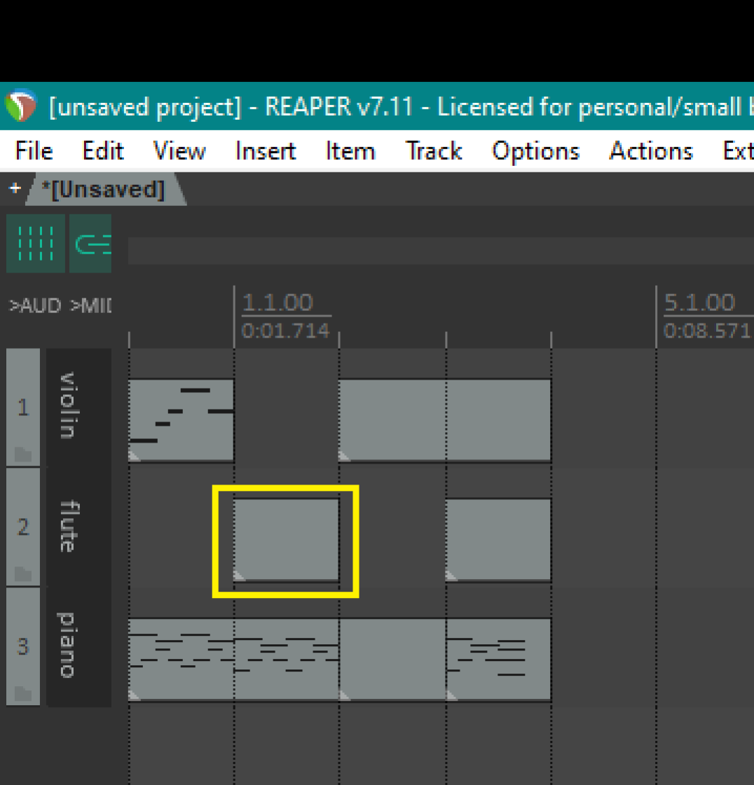
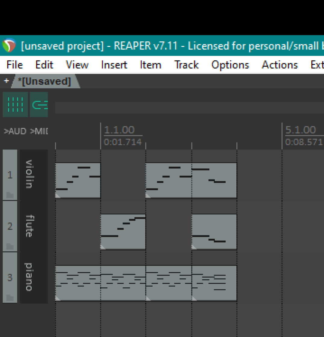
Figure 1: A 4-measure prompt in REAPER, followed by a model output. Users place empty MIDI items in REAPER to tell the model in which measures to write notes, and track names to tell the model what instrument is on each track. A track-measure in the prompt is boxed.

Composer’s Assistant (hereafter, “CA”) is a DAW-integrated multi-track MIDI infilling model. The multi-track infilling problem is the following: Given a slice of measures from a multi-track song, where the notes have been deleted from some of the track-measures (a track-measure is a measure within a track), fill in the notes for the deleted track-measures using the notes that remain as the context—see Figure 1. A model trained to complete this task without any further instruction might write parts that are musically coherent but different from what the user had in mind. For instance, a composer who generates a guitar track to accompany a drum track and bass track might receive a busy, high-pitched solo, a medium-speed, medium-pitched solo, a strummed rhythmic part, or any number of other types of outputs that may not match the composer’s intent for the track. It would be useful for the user to have the ability to condition the output on parameters such as rhythm (or, if a specific rhythm is not provided, horizontal note density instead), vertical note density, and pitch range.

In this work, we build upon CA to train a new model that offers a wide range of user controls. This work was guided by conversations with several composers who have used CA for co-creative composition, and represents an effort to remedy perceived shortcomings of that system. New controls introduced to the CA system in this work include two types of rhythmic conditioning, horizontal and vertical density controls, pitch step and leap propensity controls, several types of pitch range controls, and a rhythmic interest control. We also include a control that instructs the model not to generate octave-shifted copies of music that exists in the prompt. All of our controls are designed with a DAW-integrated interface in mind. We study the power of our controls via objective metrics, we study the extent to which the model has learned the meaning of our controls, and we conduct a listening study to evaluate music created in a co-creative fashion with our model. We release our complete, DAW-integrated system and our source code.

2 Previous Work

A wide range of generative music models predate this work, including MusicVAE [9], Piano Transformer [10], Coconet [11], and many others [12, 13, 14, 15, 16, 17, 18, 19]. FIGARO [20] explored symbolic music generation with fine-grained user control, and Music SketchNet [21] explored single-track monophonic infilling with pitch and rhythm controls.

Previous DAW-integrated models include DeepBach [22], the Piano Inpainting Application [23], and Magenta Studio [24]. Cococo [25] is a DAW-like interface to Coconet, supporting 4 tracks and arbitrary user-driven infilling/part rewriting, similar to DeepBach. NONOTO [26] is a model-agnostic interface for symbolic music infilling.

Prior multi-track infilling models include MMM [3, 4], MusIAC [27], and CA [6], all of which are transformer models. The 8-bar web demo of MMM can handle up to 6 tracks, and is limited to a 4/4 time signature. MMM has two DAW-integrated versions; however, at the time of this writing they are not publicly available. MusIAC limits inputs to 3 tracks (melody, bass, and accompaniment), 16 bars, and a collection of four time signatures. CA can handle an arbitrary collection of tracks and time signatures, provided that the time signatures contain no more than 8 quarter notes per bar. CA is integrated into the REAPER DAW, and the underlying model runs locally on the user’s machine. Each of these models offers its own set of user controls for infilling: CA offers polyphony controls, MMM offers note density and polyphony controls, and MusIAC offers five controls including note density.

In most previous works, note density is computed simply by dividing the number of notes by the number of time steps. This means that a slow part with many thick chords can have the same density as a fast monophonic part, making it difficult for a user to steer the model towards the desired rhythmic speed with a density control. Additionally, most prior works have density control sliders (with values ranging from, e.g., 1–10) whose quantiles were defined by the training data. While this approach is attractive from a training perspective, it is difficult to navigate from a user perspective—e.g., what does a density of 7/10 mean?

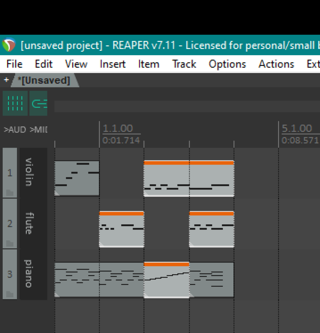
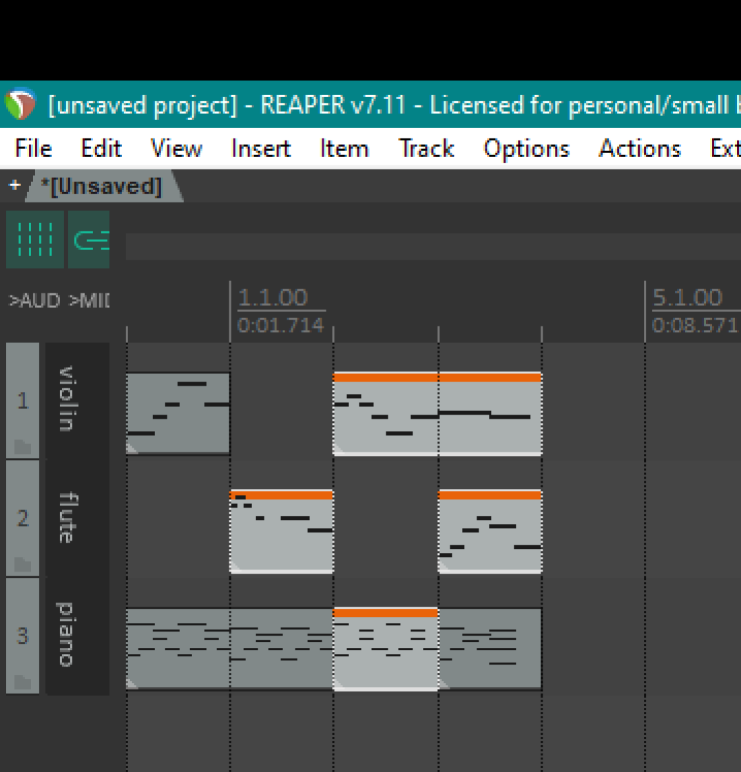
Figure 2: A prompt with 1D rhythmic conditioning in REAPER, followed by a model output. Users draw the rhythms they want in the selected MIDI items, and the model chooses pitches for these rhythms that fit with the rest of the prompt. Unselected MIDI items are included in the prompt to the encoder, and remain unchanged.

In this work, we take a different approach to note density, first by factoring note density into horizontal (rhythmic) and vertical densities, and second by adopting musically meaningful quantiles for these measurements. We note that MuseMorphose [28] also decomposed note density into horizontal and vertical densities, albeit with a different definition of vertical density (in their work, “polyphony score”) than ours. We also develop a wide range of additional steering controls, including a user option for explicit rhythmic control. With this option, the user can supply rhythms in their model prompts, and the model chooses only the pitches—see Figure 2. To our knowledge, the controls we implement in this paper comprise the most comprehensive and user-friendly set of steering controls for multi-track MIDI infilling to date.

3 Measurements for User Controls

In this section we describe the measurements underlying the user controls implemented in this work. Recall that music in MIDI format is time-quantized to a uniform grid of some number of ticks per quarter note.

3.1 Horizontal Measurements

Horizontal note onset density. We define the horizontal note onset density of a collection of measures from a track to be the number of ticks with a note onset divided by the total number of ticks. In interval notation, we quantize horizontal note onset densities to the following six bins: Less than half notes; $[$Half notes, Quarter notes$)$; $[$Quarter notes, Eighth notes$)$; $[$Eighth notes, 16th notes$)$; $[$16th notes, 4.5 onsets per quarter note$)$; $\geq$ 4.5 onsets per quarter note.

Rhythmic interest. Given a slice of measures from a track, let $v$ denote the binary rhythm vector of those measures. Let $\hat{v}=v-\bar{v}$ denote $v$, re-centered at 0. We compute dot products of $\hat{v}$ with its nontrivial shifts and record the highest of their absolute values as a measure of rhythmic uniformity. Rhythmic uniformity is scaled by $1/||\hat{v}||^{2}$ and subtracted from 1 to yield rhythmic interest, which we divide into Low ($<0.14$), Medium ($\geq 0.14$ and $<0.4$), and High ($\geq 0.4$) bins. These quantiles were hand-selected by looking at many examples. See Figure 3 for examples.

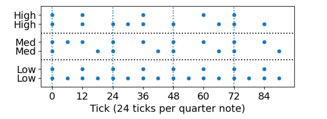
Figure 3: Six examples of rhythmic interest levels. Points mark note onsets in a 4/4 measure.

3.2 Vertical Measurements

Vertical note onset density. We define the vertical note onset density of a collection of track-measures from a track to be the number of notes divided by the number of ticks containing an onset. In interval notation, we quantize vertical note onset densities into the following five bins: 1 note per onset; (1 note per onset; 2 notes per onset]; (2 notes per onset, 3 notes per onset]; (3 notes per onset, 4 notes per onset]; $>$ 4 notes per onset.

Average number of pitch classes per note onset. This measure is the same as vertical note onset density, but with pitches replaced with pitch classes. It is $(\sum_{t}\#\textup{pitch classes at }t)/\#\textup{ticks containing an onset}$. We use the same bins as vertical note onset density: 1 pitch class per onset; (1 pitch class per onset, 2 pitch classes per onset]; (2 pitch classes per onset, 3 pitch classes per onset]; (3 pitch classes per onset, 4 pitch classes per onset]; $>$ 4 pitch classes per onset.

3.3 Pitch Measurements

Pitch step and leap propensity. Given two consecutive notes, a step is a difference in pitch of 1–2 semitones, while a leap is a difference of more than 2 semitones. Pitch repetitions are neither steps nor leaps. We generalize to chords as follows: Given a chord $C_{1}$ followed by a chord $C_{2}$, define the chord distance $d(C_{1},C_{2})$ to be the average of the minimum pitch movements needed to get from the notes in $C_{1}$ to the notes in $C_{2}$:

$$d(C_{1},C_{2})=\frac{1}{|C_{1}|}\sum_{n_{1}\in C_{1}}\min_{n_{2}\in C_{2}}|\textup{pitch}(n_{1})-\textup{pitch}(n_{2})|.$$

Going from a chord $C_{1}$ to a chord $C_{2}$, we have a repetition when $d(C_{1},C_{2})=0$, a step when $0<d(C_{1},C_{2})\leq 2$, and a leap when $d(C_{1},C_{2})>2$. Given a slice of measures from a track containing $n$ chords, we count the number of steps and leaps and divide by $n-1$ to obtain the pitch step propensity and pitch leap propensity for the slice. We quantize pitch step and leap propensities into the following seven bins: $[0,0.01)$, $[0.01,0.2)$, $[0.2,0.4)$, $[0.4,0.6)$, $[0.6,0.8)$, $[0.8,0.99)$, $[0.99,1.0]$.

Note onset chromagrams. When prompted to generate new tracks to accompany an arrangement already containing several tracks, we observed that the CA model would often generate a copy (possibly shifted by some number of octaves) of one of the tracks in the prompt. While this is often “correct,” it is not particularly useful for co-creative composition—if that is what the composer wanted, they could easily create this themselves. To create a control that tells the model to write genuinely new parts, for each track-measure in a song, we record whether that track-measure has the same note onset chromagram as another track-measure in its measure. (Given a track-measure $T$, the set of ordered pairs $\{(\textup{pitch}(n)(\textup{mod }12),\textup{onset tick}(n)):n\textup{ is a note whose onset is in }T\}$ is the note onset chromagram of $T$.)

3.4 Other Measurements

Pitch range. The pitch range of a collection of track measures is simply a record of their lowest and highest pitch.

Rhythmic information. We define the 1D rhythmic information of a collection of measures from a track to be the set of note onset ticks and corresponding note durations after flattening all notes to the same pitch. If multiple notes share an onset, we record only the longest of their durations. The 2D rhythmic information of a collection of measures from a track is the same, but with the number of note onsets and number of pitch classes at each onset also recorded.

4 Controls and Model

We use the MIDI-like token-based language from [6] to tokenize music. This language supports masking of arbitrary subsets of track-measures from any slice of measures from a song. We add additional tokens to the language to serve as control tokens for the measurements introduced in Section 3. For each of the measurements that are quantized into bins in Sections 3.1–3.3, for each bin, we create a separate control token. We also create a control token to indicate when a track-measure has a different note onset chromagram from all other track-measures in its measure—we call this token the different-note-onset-chromagram (DNOC) token. We also create pitch range controls and explicit rhythmic controls. For pitch range control, we create four control tokens: high (strict), low (strict), high (loose), and low (loose), and we follow such a token by a pitch token to indicate the value of the measurement. With strict pitch range controls, which can be supplied on a per-track or per-track-measure basis, the model is expected to generate at least one pitch at each extreme. With loose pitch range conditioning, the model is expected to generate at least one note within 7 semitones of each extreme and not extend beyond the extremes. The idea is that a user could supply a loose pitch range for, e.g., a vocal melody, whose bounds are given by the range of the vocalist. For rhythmic conditioning, we create masked pitch tokens, which are included with rhythmic tokens (describing note onset position and note duration) in prompts. For 1D rhythmic conditioning, we include a single masked pitch token at each tick containing any number of note onsets. For 2D rhythmic conditioning, we include masked pitch tokens describing both the number of note onsets and the number of pitch classes at each onset.

As in [6], we train a T5-like [29] encoder-decoder transformer [30] model. Our main model (which we refer to as our large model) is 512-dimensional, with 16 encoder layers and 16 decoder layers. This model has about 3.5$\times$ the number of parameters of the CA model, which is 384-dimensional, with 10 encoder layers and 10 decoder layers. To examine the effect of model scaling on performance, we also train a small model having the same dimension and number of layers as the CA model. For inference, we use nucleus sampling [31] with a threshold of $p=0.85$.

During training, we mask a random subset of track-measures from a slice of measures within a song, and we ask our model to generate the tokens for the masked track-measures. All unmasked track-measures within the slice are included in the prompt provided to the encoder. In each example, we include a random subset of our control tokens in our prompts. Control tokens operating on the track level are appended to the prompt, while control tokens operating on the track-measure level are inserted into the prompt in place of the masked tokens that the model is asked to generate. For training, values for control tokens are computed using only the masked track-measures. For inference, this allows a user to specify attributes for track-measures to be filled that differ arbitrarily from the attributes of the unmasked track-measures in the prompt. During inference in the DAW, we apply only the control tokens supplied by the user.

We quantize music to a mixed grid that accommodates 32nd notes and 16th note triplets. This grid has 24 ticks per quarter note, of which 12 are valid locations for note onsets. To train our models, we use the CA training dataset (a dataset of public-domain and permissively-licensed MIDI files). As in [32], we take the “e” folder of the Lakh MIDI dataset (LMD) [33, 34] to be our validation set.

5 Evaluation

In [6], CA generally outperformed MMM [3, 4] on objective and subjective measures. However, whether this was due to training approach, training dataset, model size, and/or other factors is unclear. To make a direct comparison between our work and previous work, we adopt CA as our baseline for comparison on objective metrics.

Model $\backslash$ Task	Random	Track	Last-bar
	infill	infill	fill
Note $F_{1}$ results $\uparrow$
CA2 large	77.01a	70.74a	78.34a
CA2 small	76.27b	69.67b	77.24b
CA	52.59c	31.65c	53.74c
Precision $\uparrow$
CA2 large	77.15a	70.85a	78.45a
CA2 small	76.39b	69.78b	77.35b
CA	53.02c	33.76c	54.72c
Recall $\uparrow$
CA2 large	76.90a	70.64a	78.24a
CA2 small	76.15b	69.58b	77.15b
CA	52.67c	32.22c	53.75c
Pitch class histogram entropy difference $\downarrow$
CA2 large	10.78a	14.69a	8.90a
CA2 small	11.28b	15.49b	9.75b
CA	31.65c	50.53c	31.60c
Groove similarity $\uparrow$
CA2 large	99.97b	99.97a	99.97a
CA2 small	99.98a	99.97a	99.98a
CA	97.84c	96.01b	97.87b

Table 1: Objective infilling summary statistics. All cells are percentages of the form mean^s, where $s$ is a letter. Different letters within a metric and column indicate significant location differences ($p<0.01$) in the samples for those table entries according to a Wilcoxon signed rank test with Holm-Bonferroni correction.

5.1 Objective Evaluation

We take the “f” folder of the LMD to be our test set. From each file, we select random 8-measure slices and attempt to prepare three test examples:

• Random infilling: Each track-measure in the slice is masked with probability 0.5.

• Track infilling: One track from the slice, containing note onsets in at least 7 measures, is masked completely.

• Last-bar infilling: Every track-measure in the last measure of the slice is masked.

We take 5000 examples of each type of infilling to be our test set. For each example, we take the masked notes to be the ground truth, and after evaluating the example with our models we compute precision and recall as in [6]. The $F_{1}$ score for an example is the harmonic mean of its precision and recall: $F_{1}=(2\cdot\textup{precision}\cdot\textup{recall})/(\textup{precision}+\textup{recall})$. We also compute the pitch class histogram entropy difference and the groove similarity (as defined in [35]) between the ground truth and the output for each example.

We evaluate our test examples with our models, providing user controls describing the information in the masked track-measures to the maximum extent possible. In particular, we provide 2D rhythmic conditioning, pitch step and leap propensity, pitch range per track-measure, and the DNOC token (wherever applicable) to our models. Results are averaged and presented in Table 1. For examples evaluated by CA, we provide all of the control information available to that model—in particular, mono/poly switches at the track-measure level. We note that supplying rhythmic conditioning and pitch range information for track-measures containing only one pitch is equivalent to unmasking those track-measures. Therefore, to make a fair comparison between our models and CA, we unmask those track-measures in our prompts to CA and we give that model “credit” for those track-measures as if it had generated them itself. (14.46% of the track-measures from our test set fall into this category.) We see a dramatic increase in performance of our models relative to CA. As expected, our large model outperforms our small model (except for groove similarity for the random infilling task), but the differences in performance between our models are small. Note that the groove similarity score for our models is not 100%, indicating that our models sometimes (albeit rarely) fail to follow exactly the rhythms in their prompts.

Next, we examine the effect of each control introduced in this paper by repeating our test examples, but with only limited control information supplied to the model. For each control introduced in this paper, we examine the $F_{1}$ scores obtained by supplying only that control to the model. We also examine what happens when we supply a growing collection of controls, roughly in order of how much effort is required for a user to supply such controls in practice—specifically, we supply, in order: vertical controls, horizontal controls, our DNOC control, pitch/step leap controls, pitch range (per track), 1D rhythmic conditioning, 2D rhythmic conditioning, and finally pitch range (per track-measure). The resulting large table of $F_{1}$ scores is omitted, but the primary observation is that pitch range and rhythmic conditioning controls have the largest positive effect on the $F_{1}$ scores of model outputs. Model size has only a minor effect. Horizontal, vertical, pitch step/leap propensity, and DNOC controls also have only minor effects on $F_{1}$ scores. This raises the questions of whether the model understands the meaning of these controls and whether these controls are useful for co-creative composition, which we address in the next two sections.

5.2 Model Understanding of Control Tokens

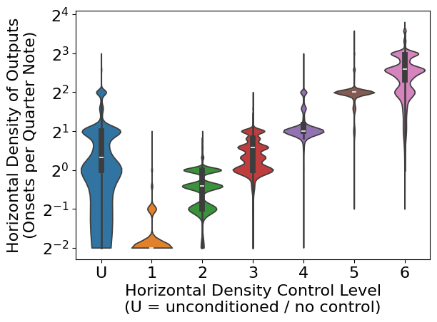
Figure 4: Horizontal density distributions.

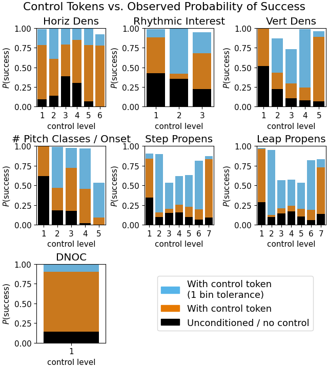
Figure 5: The observed probability of success for each control token in our empty prompting test.

Our model can generate music from scratch by prompting it with prompts containing no notes. To examine the understanding our model has of our control tokens, we use an empty prompting strategy: We prompt the model to generate some number of bars of single-track music from scratch, with no control tokens, and then we repeat the empty prompt with a single control token added. We use this approach to examine our horizontal, vertical, pitch step, pitch leap, and DNOC control tokens. For each control token we generate 5000 examples, and we examine the resulting distributions. (For the DNOC control, we use a 1-bar example where a viola and cello play an ostinato one octave apart, and prompt the model to write a violin part to accompany them.)

A plot of our horizontal note onset density distributions is given in Figure 4. Plots of other distributions are similar.

For each control token, we also compare the observed probability of obtaining an output described by that token when the token is supplied versus when it is not supplied, finding that all 34 tokens mentioned above indeed push our model towards outputs having the characteristics they are intended to encode. Probabilities of success vary, however—see Figure 5. Our DNOC token performs well, with a success rate of 90.5%, as compared to unconditioned outputs having a different note onset chromagram 14.2% of the time. Our model has also done a good job of learning the concepts of horizontal density, high and low rhythmic interest, high and low vertical density, monophonic versus polyphonic generation, and high and low step and leap propensity. However, when supplied with the appropriate control token, our model has trouble generating parts with medium rhythmic interest (with a 42% chance of success, versus 35.2% for unconditioned outputs), and with more than 4 pitch classes per onset (with a 8.92% chance of success, versus 0.04% for unconditioned outputs).

Additionally, our model has not learned the precise boundaries for our bins. For instance, when asking the model to generate a part with a horizontal density in the interval $[$Quarter notes, Eighth notes$)$, we observed that our model would often generate a straight eighth note pattern. When allowing for a tolerance of up to one bin away, though, all of our control tokens have a success rate of over 50%, and 26/34 of them have a success rate of over 80%.

Our model learned the meaning of each of these control tokens solely via natural training data. In future work, it may be possible to achieve better control token understanding performance by training on synthetic examples and/or by changing the boundaries of the bins.

5.3 Subjective Evaluation

We used our model in an iterative, co-creative fashion to create 12 snippets of music, each about 16 bars long. To create these snippets, we started with 6 pieces of real music and deleted one or more tracks in the music. We then used our model interactively to fill these deleted tracks. Specifically, each time the model generated music, we kept the generated track-measures we liked, and continued using the model to fill the remaining track-measures until done. We carried out this process under two sets of rules:

• CA-: We did not use rhythmic conditioning, and did not hand-edit the notes in any outputs.

• CA+: We were allowed to use every control available, including rhythmic conditioning, and we were allowed to make small hand edits to outputs. This is the approach closest to how the model would be used in practice.

In both cases we were allowed as many generations as we wanted. We recorded the creation of these examples, which took about 2 hours in total. Volunteers were asked to score as many of these 18 snippets of music as they wished, according to perceived Rhythmic correctness, Pitch correctness, Memorability, and Overall, each on a scale of 0 to 4. Volunteers were not told which pieces of music were real and which were composed with our system. 28 individuals volunteered and ranked an average of 10.4 snippets along each of our 4 axes. Aggregated results are presented in Figure 6. Each bar in this figure represents 94–99 data points.

We compare real music to music composed with our two approaches CA- and CA+ with paired $t$-tests, using data from whenever a volunteer ranked both. Each of these 8 tests involved 93–96 pairs of values. See Table 2. After Holm-Bonferroni correction, we do not find a significant ($p<0.05$) difference between real music and music composed with either approach in any of these 8 tests. We know that our model is competent at avoiding rhythmic and pitch errors, so we are not surprised by our R and P results. However, we had some difficulty creating a proper drum part in one example with the CA- approach, and we expected to find at least one significant M or O difference. We suspect that there are subjective quality differences, at least between real music and the music we created with the CA- approach, that are not large enough for this study to detect reliably. Nevertheless, we believe that this indicates that music co-created with our model has the potential to be on par with human-composed music. We also believe that results of similar studies would vary greatly depending on the skill of the composer using the system. We invite the reader to listen to our samples and to try our system.

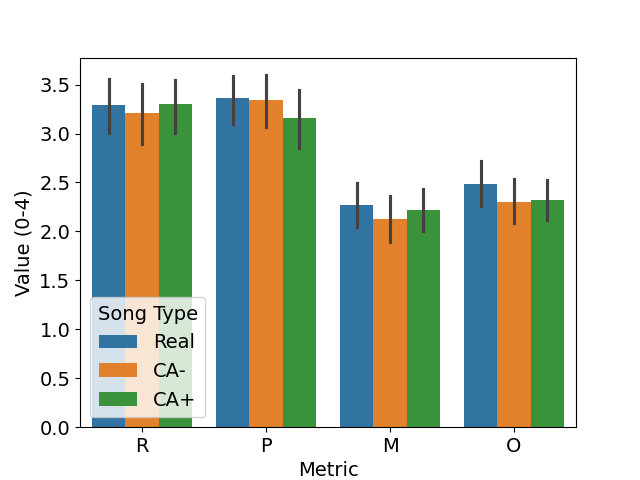
Figure 6: Subjective evaluation of our model.

Metric		Real
R	CA-	$0.693$
	CA+	$0.887$
P	CA-	$0.791$
	CA+	$0.211$

Metric		Real
M	CA-	$0.052$
	CA+	$0.422$
O	CA-	$0.039$
	CA+	$0.099$

Table 2: Uncorrected $p$-values from paired $t$-tests in our subjective comparisons.

6 Conclusion

We have introduced a wide range of steering controls for multi-track MIDI infilling, and we have trained a transformer model to implement these controls. We have created an interface for our controls, and we have integrated our model and controls into the REAPER digital audio workstation for co-creative symbolic music composition. Our work in this paper comprises Composer’s Assistant 2, and we have released our complete system and source code.

7 Ethics Statement

There are currently unresolved ethical and legal questions regarding the inclusion of copyrighted data in training sets for generative models. While we suspect it would be possible to obtain better objective (and possibly subjective) results by training a model on a larger and more varied dataset (e.g., the Lakh MIDI dataset [33, 34]), we chose to train our models only on copyright-free and permissively licensed files, primarily for the following two reasons:

First, we want our model outputs to be usable by composers. While there is a possibility that our models may output copyrighted musical information (even if such information was not present in the training dataset), we believe that training only on copyright-free and permissively-licensed musical data minimizes this possibility.

Second, for many composers, we view the models that we have released not as the models that the composers would actually use in their work, but rather as starting points for customization and personalization. Many composers we have spoken to have said that models that write “generic” music are not useful to them. Instead, they want generative systems that can suggest ideas in their own style. Due to our training set, the models we have released are most proficient at infilling classical, choral, and folk music. However, informal experiments suggest that our models can be finetuned on a relatively small number of MIDI files to write in the style of those files, and hence the style limitations of our released models may not matter. The code we have released supports finetuning by end users. While this can benefit composers who wish to use our system, there is also the risk that our models may be finetuned by users to impersonate the styles of others.

References

- [1] M. Newman, L. Morris, and J. H. Lee, “Human-AI Music Creation: Understanding the Perceptions and Experiences of Music Creators for Ethical and Productive Collaboration,” in Proc. 24th Int. Society for Music Information Retrieval Conf., Milan, Italy, 2023, pp. 80–88.
- [2] C.-Z. A. Huang, H. V. Koops, E. Newton-Rex, M. Dinculescu, and C. J. Cai, “AI Song Contest: Human-AI Co-Creation in Songwriting,” in Proc. 21st Int. Society for Music Information Retrieval Conf., Montréal, Canada, 2020, pp. 708–716.
- [3] J. Ens and P. Pasquier, “MMM : Exploring Conditional Multi-Track Music Generation with the Transformer,” arXiv preprint arXiv: 2008.06048, 2020.
- [4] ——, “Flexible Generation with the Multi-Track Music Machine,” in Extended Abstracts for the Late-Breaking Demo Session of the 21st Int. Society for Music Information Retrieval Conf., Montréal, Canada, 2020.
- [5] R. B. Tchemeube, J. Ens, C. Plut, P. Pasquier, M. Safi, Y. Grabit, and J.-B. Rolland, “Evaluating Human-AI Interaction via Usability, User Experience and Acceptance Measures for MMM-C: A Creative AI System for Music Composition,” in Proc. 32nd Int. Joint Conf. Artificial Intelligence, 2023, pp. 5769–5778.
- [6] M. Malandro, “Composer’s Assistant: An Interactive Transformer for Multi-Track MIDI Infilling,” in Proc. 24th Int. Society for Music Information Retrieval Conf., Milan, Italy, 2023, pp. 327–334.
- [7] “Andromeda | AI Opera,” September 2 , 2023. [Online]. Available: https://www.valdovurumai.lt/lt/renginiai/item/8413/
- [8] “InMuse Vilnius | Day 3 | Forum on Innovation in Music, Stage Arts and Entertainment,” 2023. [Online]. Available: https://www.youtube.com/watch?v=je7sUtPNyRs&t=12100s
- [9] A. Roberts, J. Engel, C. Raffel, C. Hawthorne, and D. Eck, “A Hierarchical Latent Vector Model for Learning Long-Term Structure in Music,” in Proc. 35th Int. Conf. Machine Learning, ser. Proceedings of Machine Learning Research, J. Dy and A. Krause, Eds., vol. 80. PMLR, 10–15 Jul 2018, pp. 4364–4373.
- [10] C.-Z. A. Huang, A. Vaswani, J. Uszkoreit, I. Simon, C. Hawthorne, N. Shazeer, A. M. Dai, M. D. Hoffman, M. Dinculescu, and D. Eck, “Music Transformer,” in Int. Conf. Learning Representations, 2019.
- [11] C.-Z. A. Huang, T. Cooijmans, A. Roberts, A. Courville, and D. Eck, “Counterpoint by Convolution,” in Proc. 18th Int. Society for Music Information Retrieval Conf., Suzhou, China, 2017, pp. 211–218.
- [12] C. Payne, “MuseNet,” openai.com/blog/musenet, 2019.
- [13] J. Liu, Y. Dong, Z. Cheng, X. Zhang, X. Li, F. Yu, and M. Sun, “Symphony Generation with Permutation Invariant Language Model,” in Proc. 23rd Int. Society for Music Information Retrieval Conf., Bengaluru, India, 2022, pp. 551–558.
- [14] S. Wei, G. Xia, Y. Zhang, L. Lin, and W. Gao, “Music Phrase Inpainting Using Long-Term Representation and Contrastive Loss,” in IEEE Int. Conf. Acoustics, Speech and Signal Processing, 2022, pp. 186–190.
- [15] A. Pati, A. Lerch, and G. Hadjeres, “Learning to Traverse Latent Spaces for Musical Score Inpainting,” in Proc. 20th Int. Society for Music Information Retrieval Conf., Delft, The Netherlands, 2019, pp. 343–351.
- [16] C. Benetatos and Z. Duan, “Draw and Listen! A Sketch-Based System for Music Inpainting,” Trans. Int. Society for Music Information Retrieval, vol. 5, no. 1, pp. 141–155, 2022.
- [17] C.-J. Chang, C.-Y. Lee, and Y.-H. Yang, “Variable-Length Music Score Infilling via XLNet and Musically Specialized Positional Encoding,” in Proc. 22nd Int. Society for Music Information Retrieval Conf., online, 2021, pp. 97–104.
- [18] G. Mittal, J. Engel, C. Hawthorne, and I. Simon, “Symbolic Music Generation with Diffusion Models,” in Proc. 22nd Int. Society for Music Information Retrieval Conf., online, 2021, pp. 468–475.
- [19] L. Min, J. Jiang, G. Xia, and J. Zhao, “Polyffusion: A diffusion model for polyphonic score generation with internal and external controls,” in Proceedings of the 24th International Society for Music Information Retrieval Conference, ISMIR, 2023.
- [20] D. von Rütte, L. Biggio, Y. Kilcher, and T. Hofmann, “FIGARO: Controllable music generation using learned and expert features,” in Int. Conf. Learning Representations, 2023.
- [21] K. Chen, C. i Wang, T. Berg-Kirkpatrick, and S. Dubnov, “Music SketchNet: Controllable Music Generation via Factorized Representations of Pitch and Rhythm,” in Proc. 21st Int. Society for Music Information Retrieval Conf., Montréal, Canada, 2020, pp. 77–84.
- [22] G. Hadjeres, F. Pachet, and F. Nielsen, “DeepBach: a Steerable Model for Bach Chorales Generation,” in Proc. 34th Int. Conf. Machine Learning, ser. Proceedings of Machine Learning Research, D. Precup and Y. W. Teh, Eds., vol. 70. PMLR, 06–11 Aug 2017, pp. 1362–1371.
- [23] G. Hadjeres and L. Crestel, “The Piano Inpainting Application,” arXiv preprint arXiv: 2107.05944, 2021.
- [24] A. Roberts, C. Kayacik, C. Hawthorne, D. Eck, J. Engel, M. Dinculescu, and S. Nørly, “Magenta Studio: Augmenting Creativity with Deep Learning in Ableton Live,” in Proc. Int. Workshop on Musical Metacreation (MUME), 2019.
- [25] R. Louie, A. Coenen, C. Z. Huang, M. Terry, and C. J. Cai, “Novice-AI Music Co-Creation via AI-Steering Tools for Deep Generative Models,” in Proceedings of the 2020 CHI Conference on Human Factors in Computing Systems, ser. CHI ’20. New York, NY, USA: Association for Computing Machinery, 2020, p. 1–13. [Online]. Available: https://doi.org/10.1145/3313831.3376739
- [26] T. Bazin and G. Hadjeres, “NONOTO: A Model-agnostic Web Interface for Interactive Music Composition by Inpainting,” in Proc. 10th Int. Conf. Computational Creativity, 2019.
- [27] R. Guo, I. Simpson, C. Kiefer, T. Magnusson, and D. Herremans, “MusIAC: An Extensible Generative Framework for Music Infilling Applications with Multi-level Control,” in Artificial Intelligence in Music, Sound, Art and Design. EvoMUSART 2022. Lecture Notes in Computer Science, T. Martins, N. Rodríguez-Fernández, and S. M. Rebelo, Eds., vol. 13221. Springer, Cham, 2022, pp. 341–356.
- [28] S.-L. Wu and Y.-H. Yang, “MuseMorphose: Full-Song and Fine-Grained Piano Music Style Transfer with One Transformer VAE,” IEEE/ACM Transactions on Audio, Speech, and Language Processing, vol. 31, pp. 1953–1967, 2023.
- [29] C. Raffel, N. Shazeer, A. Roberts, K. Lee, S. Narang, M. Matena, Y. Zhou, W. Li, and P. J. Liu, “Exploring the Limits of Transfer Learning with a Unified Text-to-Text Transformer,” Journal of Machine Learning Research, vol. 21, no. 140, pp. 1–67, 2020.
- [30] A. Vaswani, N. Shazeer, N. Parmar, J. Uszkoreit, L. Jones, A. N. Gomez, Ł. Kaiser, and I. Polosukhin, “Attention is All you Need,” in Advances in Neural Information Processing Systems, I. Guyon, U. V. Luxburg, S. Bengio, H. Wallach, R. Fergus, S. Vishwanathan, and R. Garnett, Eds., vol. 30. Curran Associates, Inc., 2017.
- [31] A. Holtzman, J. Buys, L. Du, M. Forbes, and Y. Choi, “The Curious Case of Neural Text Degeneration,” in Int. Conf. Learning Representations, 2020.
- [32] J. Thickstun, D. L. W. Hall, C. Donahue, and P. Liang, “Anticipatory Music Transformer,” Transactions on Machine Learning Research, 2024. [Online]. Available: https://openreview.net/forum?id=EBNJ33Fcrl
- [33] C. Raffel, “Learning-Based Methods for Comparing Sequences, with Applications to Audio-to-MIDI Alignment and Matching,” Ph.D. dissertation, 2016.
- [34] ——, “The Lakh MIDI Dataset v0.1,” https://colinraffel.com/projects/lmd/.
- [35] S.-L. Wu and Y.-H. Yang, “The Jazz Transformer on the Front Line: Exploring the Shortcomings of AI-Composed Music Through Quantitative Measures,” in Proc. 21st Int. Society for Music Information Retrieval Conf., Montréal, Canada, 2020, pp. 142–149.