[1]\fnmM.-J. \surChoi
1]\orgdivChair of Structural Analysis and Dynamics, \orgnameRWTH Aachen University, \orgaddress\streetMies-van-der-Rohe Str. 1, \cityAachen, \postcode52074, \countryGermany
2]\orgdivInstitute for Structural Mechanics, \orgnameRuhr University Bochum, \orgaddress\streetUniversitätsstraße 150, \cityBochum, \postcode44801, \countryGermany
3]\orgdivFaculty of Civil and Environmental Engineering, \orgnameGdańsk University of Technology, \orgaddress\streetul. Narutowicza 11/12, \cityGdańsk, \postcode80-233, \countryPoland
4]\orgdivDepartment of Mechanical Engineering, \orgnameIndian Institute of Technology Guwahati, \orgaddress\streetAssam 781039, \countryIndia
An objective isogeometric mixed finite element formulation for nonlinear elastodynamic beams with incompatible warping strains
Abstract
We present a stable mixed isogeometric finite element formulation for geometrically and materially nonlinear beams in transient elastodynamics, where a Cosserat beam formulation with extensible directors is used. The extensible directors yields a linear configuration space incorporating constant in-plane cross-sectional strains. Higher-order (incompatible) strains are introduced to correct stiffness, whose additional degrees-of-freedom are eliminated by an element-wise condensation. Further, the present discretization of the initial director field leads to the objectivity of approximated strain measures, regardless of the degree of basis functions. For physical stress resultants and strains, we employ a global patch-wise approxiation using B-spline basis functions, whose higher-order continuity enables to use much less degrees-of-freedom, compared to element-wise approximation. For time-stepping, we employ an implicit energy–momentum consistent scheme, which exhibits superior numerical stability in comparison to standard trapezoidal and mid-point rules. Several numerical examples are presented to verify the present method.
keywords:
Beam, Extensible directors, Objectivity, Mixed formulation, Warping, Implicit dynamics1 Introduction
A Cosserat beam represents a slender object described by a spatial curve with two attached directors at each material point. Those directors span the (planar) cross-section, and are often assumed to be orthonormal, so that they can be parameterized by three rotational parameters. It has been shown that a standard finite element approximation of three-dimensional rotation parameters can lead to a loss of frame-invariance of the underlying continuous strains, due to the non-additive nature of finite rotations, see Crisfield and Jelenić [11] and Jelenić and Crisfield [20] for the relevant investigation and its remedies using the concept of local rotation. For a comprehensive review of different types of rotational parameterizations for nonlinear beams, one may refer to Romero [32]. It has also been shown that a direct finite element approximation of the director vectors can circumvent this issue, which, however, requires an additional constraint for the directors’ orthonormality. For example, this constraint can be imposed at the nodal points by using a Lagrange multiplier method [2], or introducing nodal rotational parameters [18, 33]. On the other hand, this orthonormality constraint can be simply abandoned, so that one has two independent extensible (unconstrained) directors, which represent in-plane shear and transverse normal strains of the cross-section. This increases the number of degrees-of-freedom (DOFs) per cross-section from six to nine, but the configuration space becomes linear, . The relevant approaches can be found, e.g., in Rhim and Lee [31], Coda [10], Durville [13], and Choi et al. [8]. Note that these approaches based on a direct finite element approximation of the director field may have a singularity in coarse meshes, when the directors’ orientation changes abruptly along the length [32, Section 4.3]. The direct finite element approximation of (total) directors implies that the initial director field is also approximated. A continuous (exact) representation of the initial director field, inconsistent from the finite element approximation, may lead to a loss of objectivity. In Choi et al. [9, Sec. 6.2] it turned out that using a reduced degree of basis for the change of directors lower than that of the initial (continuous) director field may result in the inability to represent rigid body rotations. In the present paper, we present a finite element approximation of the initial director field such that the objectivity is satisfied for any degree . For the relevant discussion on the objectivity under Kirchhoff beam kinematics, we refer interested readers to Meier et al. [26].
(Out-of-plane) warping means a cross-sectional deformation such that an initially planar cross-section does not remain plane. It can be coupled with other deformation modes like bending, shear, or torsion. In order to take this into account in Timohsenko beam kinematics, Simo and Vu-Quoc [38] introduced an additional DOF representing the amplitude of warping, and it is multiplied by a pre-defined warping function to produce an out-of-plane displacement, which has also been applied in the framework of unconstrained directors in Coda [10]. This has been extended by Klinkel and Govindjee [23] to deal with anisotropic linear elastic materials which exhibits a bending–torsion coupling. In these previous works, the additional DOF for warping leads to non-standard stress resultants, bi–moment and bi–shear in the equilibrium equations. See also Nukala and White [29] for a relevant approach with simplified shear strains such that the transverse shear strain and the warping shear strain due to non-uniform torsion are neglected. In the framework of an enhanced assumed strain (EAS) method [35], one can enhance the cross-sectional strains that do not exist in the compatible strain field from the configuration. This requires additional constraints like orthogonality between the enhanced strain and the stress field. Wackerfuß and Gruttmann [40] presented a construction of global polynomial basis functions of an arbitrary order for the enhanced cross-sectional strains. This has been extended to incorporate an arbitrary (open) cross-section shapes by using a local polynomial basis in Wackerfuß and Gruttmann [41], which has also been employed in Klarmann et al. [22] for a coupling between beam and brick elements. In the present work, the construction of global polynomial basis functions need to be more generalized, in order to account for the additional deformation modes in the compatible strain field such as transverse normal and in-plane shear strains, due to the extensible (unconstrained) directors. An alternative way to incorporate warping, which, however, requires increased number of global DOFs, is to use higher-order directors [28, 7]. One may also consider using multiple brick (solid beam) elements in the cross-section, e.g., as in Frischkorn and Reese [15].
The total linear momentum, total angular momentum, and total energy are fundamental integral quantities of motion in nonlinear elastodynamics, and their conservation (under suitable boundary conditions) manifests the stability of a numerical time-stepping scheme. For nonlinear problems, the standard trapezoidal rule, corresponding to and in the Newmark family, preserves the total linear momentum but neither the total angular momentum nor the total energy [36]. The standard mid-point rule preserves both of the total linear and angular momentums but not the total energy [16]. It has been shown that time-stepping schemes which preserve the conservation laws underlying the time-continuous form show superior numerical stability, compared with standard ones like the trapezoidal and mid-point rules. A class of these energy–momentum consistent (EMC) algorithms can be obtained by modifying the (implicit) mid-point rule. For example, one may refer to the algorithmic treatment of the stress resultant in Romero and Armero [33], and Betsch and Janz [1] for geometrically nonlinear beam and shell problems, respectively, and Gonzalez [16] for general (nonlinear) hyperelastic materials.
The remainder of this paper is organized as follows. In Section 2, we introduce the beam kinematics based on the extensible directors. Section 3 presents a mixed variational formulation for nonlinear dynamics of beams, which includes an EAS method for enriching higher-order cross-sectional strains. Section 4 presents an implicit time-stepping scheme for energy–momentum consistency. Section 5 presents an isogeometric spatial discretization. In Section 6, several numerical examples are presented. Section 7 concludes the paper.
2 Beam kinematics
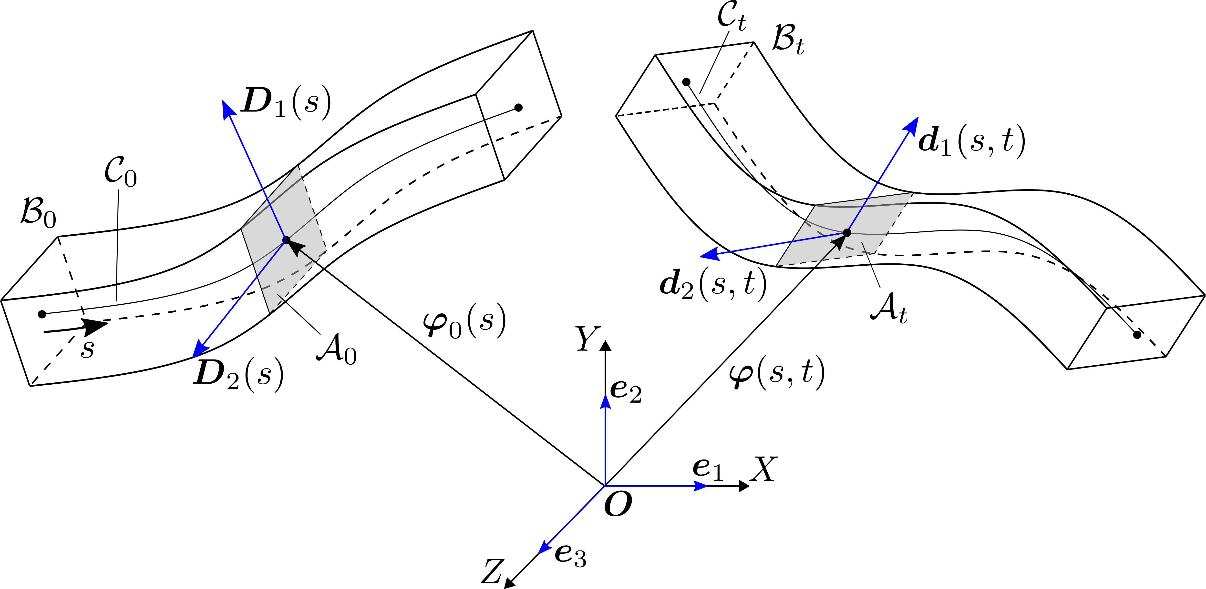
This section presents the kinematical description of Cosserat beams, based on extensible directors, and the resulting configuration–strain relation. A beam characterizes a three-dimensional body whose dimension along the longitudinal direction is much larger than the others such that a suitable kinematical assumption on the cross-sectional deformation can be employed. The origin of the transverse coordinates is given by the geometrical center of the initial cross-section, which coincides with the mass center, assuming constant mass density in the initial configuration. The line connecting these center points is called an initial center axis whose position is represented by the vector , , where denotes its arc-length coordinate, and denotes its length. Then, the initial beam configuration can be expressed by
| (1) |
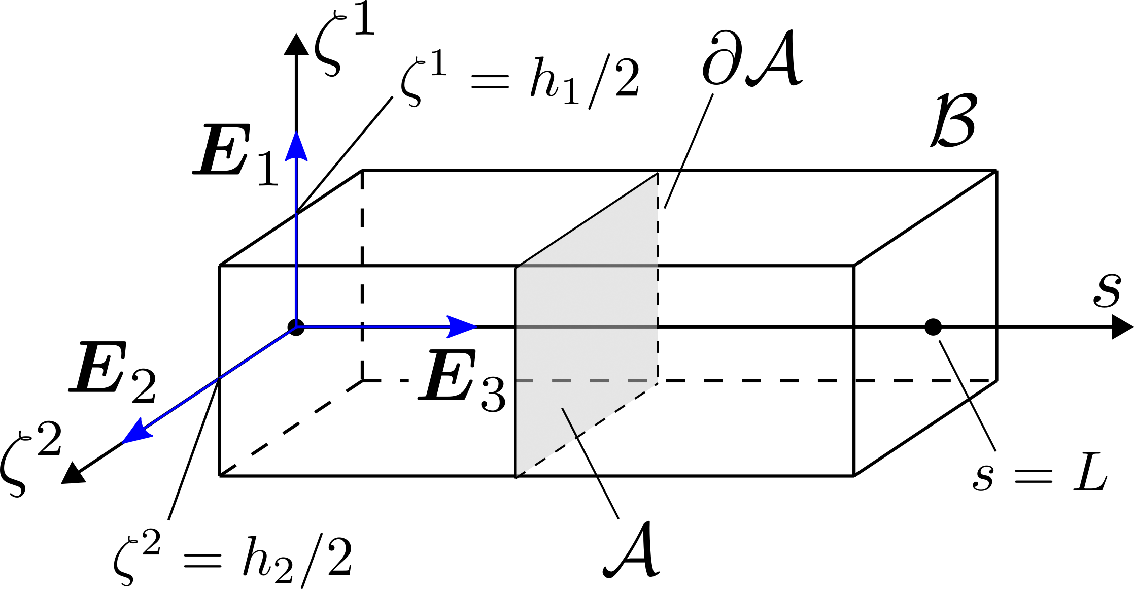
where the two orthonormal vectors are called initial directors, and they span the initial cross-sectional plane, in Fig. 1. Those initial directors are defined along two principal directions of the cross-section’s second moment of inertia. Here and hereafter, unless stated otherwise, repeated Greek indices like , , and imply summation over to , and repeated Latin indices like and imply summation over to . The initial directors are unit vectors and dimensionless, such that the cross-sectional dimension is associated with the range of the transverse coordinates , where denotes the (open) domain of the (initial) cross-section and denotes its boundary, see Fig. 2. It should be noted that the transverse coordinates are independent of time. In the initial configuration, we define the covariant basis with , and the contravariant basis can then be uniquely determined by the orthogonality condition , where denotes the Kronecker-delta.
Remark 2.1:
Initial curvature. The initial covariant base vectors are obtained by [8]
| (2) |
The infinitesimal volume in the initial configuration can be decomposed into
| (3) |
where the Jacobian is expressed by
| (4) |
with
| (5) |
which is associated with the initial curvature of the center axis, for a given initial center axis curve and the attached initial directors . Note that, for initially straight beams or linear elements, , so that .
We introduce the first order beam kinematics, which expresses the current position of a material point, as
| (6) |
where denotes the current position of the center axis, and the current cross-sectional plane is spanned by two current directors , see Fig. 1. Here, denotes time, where represents the terminal time. We obtain the velocity by differentiating Eq. (6) with respect to time, as
| (7) |
where the upper dot denotes the material time derivative. Hereafter, for brevity, we often omit the arguments, e.g., , and . Further, we define a configuration variable , where denotes the number of independent cross-sectional components.
2.1 Geometric strain: strain-configuration relation
We may represent a three-dimensional strain state of a beam by so called beam strains evaluated at the center axis. In the current configuration, we define the covariant basis , and then the contravariant basis can be uniquely determined by the orthogonality condition . Then, the deformation gradient tensor can be expressed by [42, page 31]
| (8) |
The Green-Lagrange strain tensor is defined by
| (9) |
where denotes the identity tensor. In Voigt notation, we have
| (10) |
where the underline denotes Voigt notation of a second order tensor, and we have defined the matrix [8]
| (17) |
and the beam strain components
| (18a) | ||||
| (18b) | ||||
| (18c) | ||||
| (18d) | ||||
| (18e) | ||||
| (18f) | ||||
| , | ||||
which are arrayed in the form
| (19) |
where denotes the number of independent strain components. Those beam strain components are called
Note that and . We call , expressed in terms of the configuration variable , a geometric strain, which represents the strain-configuration relation, whose objectivity is proved in Section A.1.
3 Mixed variational formulation
3.1 Variational forms
3.1.1 Total strain energy: Hu-Washizu principle
Based on the Hu-Washizu variational principle, the total strain energy, , can be expressed, using Eq. (3), as
| (20) |
where denotes the strain energy density per unit undeformed volume, expressed in terms of the physical (independent) Green-Lagrange strain tensor, . The compatibility condition,
| (21) |
is enforced by a Lagrange multiplier method, where the Lagrange multiplier can be interpreted as the physical second Piola-Kirchhoff stress tensor. This type of variational formulation is motivated by the following:
-
•
The introduction of an independent strain aims at an alleviation of numerical locking due to the parasitic terms in the compatible (geometric) strain from the finite element approximation of the configuration variable, .
-
•
The introduction of an independent stress field alleviates the overestimation of internal force at inequilibrium configurations, which turns out to allow much larger load increments, compared with the displacement-based formulation.
The relevant investigations can be found in, e.g., Klinkel et al. [24] for elastostatics, and Betsch and Janz [1] for elastodynamics. Further, we may enhance the physical strain field, as [35, 3]
| (22) |
where ‘tot’ means ‘total’, and the ‘kinematic’ part means its compatibility with the geometric (compatible) strain, in Eq. (21). Substituting Eq. (22) into Eq. (20), the total strain energy in Eq. (20) can be rewritten as
| (23) |
where the following orthogonality condition is utilized
| (24) |
The compatibility in Eq. (21) enables to represent the three-dimensional strain state in terms of the physical strain , as
| (25) |
as in Eq. (10). This, so called an enhanced assumed strain (EAS) method is introduced to correct stiffness, which, especially, takes the following into account:
-
•
Correction of the bending stiffness, considering the fact that a bending deformation may lead to (at least) linear in-plane cross-sectional strain, due to non-zero Poisson’s ratio,
-
•
Correction of the torsional stiffness, considering the fact that torsion may induce cross-sectional warping,
-
•
Correction of the transverse shear stiffness.
The enhanced strain can also be represented by the parameters , as
| (26) |
with the following matrix of basis functions [40]
| (33) |
where the blank entries represent zeros, and denotes the derivative with respect to (). Here, , , , and denote row arrays of the global polynomial basis functions for enriching the transverse normal (, ), in-plane shear (), axial normal (), and transverse shear (,) strains, respectively.
Remark 3.1:
For the transverse shear strains (, ), we employ the derivatives of . However, we distinguish from , which is in contrast to the formulation of Wackerfuß and Gruttmann [40]. This is due to the quadratic basis for in Eq. (17), which does not exist for and . We verify the erroneous results from using in Figs. 7 and 13(a) in Section 6.3.
The detailed process of constructing () is given in Appendix A.3. Then, the total number of independent components in the enhanced strain field is , where the dimension is given by Eq. (191). It is noted that ‘global’ implies that the basis functions span the whole domain of the cross-section, . This, however, is not suitable to represent localized warping, e.g., for a beam having an open cross-section. This limits the applicability of the present formulation to convex-shaped cross-sections like a rectangular one. In order to overcome this, one may consider the local polynomial basis functions in Wackerfuß and Gruttmann [41]. Substituting Eqs. (25) and (26) into Eq. (23) gives
| (34) |
where we define the line energy density (strain energy per undeformed unit length),
| (35) |
Here, the Lagrange multiplier
| (36) |
for the compatibility condition, , in Eq. (34) represents an array of physical stress resultants. Note that each component of the array is an independent variable, a work-conjugate to the corresponding component in the array . Taking the first variation of Eq. (34), we obtain the internal virtual work, [9]
| (37) |
where we have defined
| (38a) | ||||
| (38b) | ||||
| (38c) | ||||
| (38d) | ||||
Here denotes the first variation, and we have defined
| (39a) | |||
| (39b) | |||
| with . | |||
The detailed expression of the operator defined by
| (40) |
is given in Choi et al. [8, Eq. (A.4.5)].
3.1.2 Work function due to external loads
We define a work function for time-dependent external loads,
| (41) |
where [8]
| (42) |
Here, and () denote the given external (distributed) force and director couple along the center axis, respectively, that follow from the body force and the lateral-surface tractions. Further, and denote the prescribed force and director couple at the Neumann boundary, , due to a given surface traction acting on the end faces. denotes the empty set. Then, by taking the first variation of the work function in Eq. (41), the external virtual work at time can be expressed as
| (43) |
Note that, here, we assume that the external load is deformation-independent. If the external load has no explicit time dependence, the system is conservative, i.e., the total energy of the system is conserved [25, Sections 1.7 and 1.8], and we may define an external potential energy as
| (44) |
3.1.3 Kinetic energy
We define an independent (material) velocity vector that satisfies
| (45) |
From the beam kinematics in Eq. (7), we may also decompose the independent velocity field into two parts: the center axis velocity and the director velocity () that satisfy the compatibility condition
| (46) |
where, for brevity, we define a generalized velocity . Then, we can express the total linear momentum as
| (47) |
where we have defined the local linear momentum per undeformed unit arc-length,
| (48) |
with the mass per undeformed unit arc-length, i.e., the line mass density,
| (49) |
and the first mass moment of inertia per undeformed unit arc-length,
| (50) |
We can then express the total angular momentum, as
| (51) |
where we have defined the local director momentum per undeformed unit arc-length,
| (52) |
with the second mass moment of inertia per undeformed unit arc-length,
| (53) |
For brevity, we combine Eqs. (48) and (52) into
| (54a) | |||
| with the mass moment of inertia | |||
| (54b) | |||
| which is time-independent. It should be noted that is symmetric (i.e., ), regardless of the cross-section’s shape and initial mass distribution. | |||
Further, we define the total kinetic energy, as
| (55) |
Accordingly, we have an inertial contribution to the virtual work,
| (56) |
3.2 Euler-Lagrange equations: Hamilton’s principle
We define the Lagrangian
| (60) |
where the last term represents a weak enforcement of the constraint in Eq. (46). Here, the Lagrange multipliers can be identified by the stationarity of the Lagrangian with respect to the independent velocities and (), as [1, Section 3.2]
| (61a) | ||||
| (61b) | ||||
Substituting Eq. (61) into Eq. (60), the Lagrangian can be rewritten as
| (62) |
from which we define an action integral in the time span ,
| (63) |
By the stationarity condition of the action integral, we obtain the following weak form of the initial-boundary-value problem: Find the solution at time such that
| (64a) | ||||
| (64b) | ||||
| (64c) | ||||
| (64d) | ||||
| are satisfied for all , together with the compatibility condition from Eq. (46), | ||||
| (65) |
and the initial conditions at ,
| (66a) | |||||
| (66b) | |||||
Here, and denote the given initial velocity fields for the center axis and directors, respectively. We define the kinematically admissible solution space for the configuration variable , as
| (67) |
where denotes the Dirichlet boundary such that and . The variational space is defined as
| (68) |
Further, we employ the solution spaces for the physical variables, , and such that those solution functions may have discontinuity in the domain. Further comment on the selection of the approximation space is given in Sections 5.2.2 and 5.2.3.
4 Temporal discretization: an EMC scheme
We divide a given time span into intervals, and find approximate solutions at discrete times , where is a non-negative integer. Note that time increment can vary adaptively. We denote the approximation of the independent solution variables at time by . In the given time interval , our goal is to find an approximate solution at time for a given solution at time . We present an implicit time-stepping scheme, based on the previous work in Betsch and Janz [1], which exactly preserves the total energy for linear constitutive laws. A further extension to nonlinear constitutive laws, e.g., using the discrete derivative of Gonzalez [16] remains future work. The present time-stepping scheme turns out to exhibit superior numerical stability in comparison to standard trapezoidal and mid-point rules. We first approximate the first-order time derivatives at the mid-point, as
| (69a) | ||||
| and | ||||
| (69b) | ||||
Further, we define the mid-point approximations
| (70a) | ||||
| (70b) | ||||
| (70c) | ||||
| and | ||||
| (70d) | ||||
From the compatibility condition in Eq. (65) at the mid-point, combining Eqs. (69a) and (70d) gives [1, Sec. 3.8]
| (71) |
Then, substituting Eq. (71) into Eq. (69b) yields
| (72) |
Substituting Eq. (72) into Eq. (64), a time-discrete form of the momentum balance equation at the mid-point can be stated as:
| (73a) | ||||
| which is subject to | ||||
| (73b) | ||||
| (73c) | ||||
| (73d) | ||||
| . | ||||
It should be noted that, in Eq. (73b), we have imposed the compatibility between the displacement and the physical strain at time instead of , which is sufficient for the exact conservation of total energy for linear constitutive laws [1]. Note that this treatment is in line with using the algorithmic stress resultant in Romero and Armero [33], which evaluates the stress resultant by taking an average between two subsequent time steps, instead of evaluating it from the nonlinear strain-configuration relation at the mid-point.
4.1 Linearization
Due to the geometrical and material nonlinearities in the internal virtual work term of Eq. (3.1.1), we need an incremental-iterative (Newton-Raphson) solution process. It can be stated as: In the th time step, for the given solution at the previous th time step , and that in the previous iteration
find the solution increment
such that
| (82) | ||||
| (83) |
, and update
| (84a) | |||||||
| (84b) | |||||||
| (84c) | |||||||
| (84d) | |||||||
for , until a convergence criteria is satisfied. After the iteration finishes, we should also update the independent velocity field using Eq. (71). In Eq. (82), we have the tangent operator
| (89) |
where we have defined the constitutive matrices, as [9]
| (90a) | |||||
| (90b) | |||||
| (90c) | |||||
based on the material elasticity tensor
| (91) |
Here, denotes Voigt notation of a fourth-order tensor with major and minor symmetries. The detailed expressions of the operators and can be found in Eq. (A.4.9) and (A.4.11) of Choi et al. [8], respectively. In Eq. (89), we also employ the following averaged solution variables
| (92a) | ||||
| (92b) | ||||
| (92c) | ||||
| (92d) | ||||
Further, and denote the identity and zero matrices of dimension , respectively.
Remark 4.1:
Remark 4.2:
In Section B.2.3, we analytically verify the energy–momentum consistency of the present EMC scheme, which holds regardless of the element sizes in temporal and spatial domains.
5 Spatial discretization: an isogeometric approach
Next, we present the spatial discretization of the configuration and physical variables in the framework of an isogeometric analysis (IGA). Especially, we show that the finite element approximation of the (total) director field leads to the objectivity of the approximated (discrete) beam strain. This basically necessitates an approximation of the initial director field.
5.1 NURBS curve
In the isogeometric approach, we employ the same spline basis functions in the Computer-Aided Design (CAD) model for the analysis. This enables (i) an exact representation of the geometry of the beam’s initial center axis including conic sections like a circle, and (ii) higher-order inter-element continuity which leads to the superior per DOF accuracy, compared with the conventional –finite elements [9]. Using NURBS (Non-Uniform Rational B-spline), the beam’s initial center axis can be represented by
| (93) |
where denotes the position of the th control point, denotes the corresponding NURBS basis function of degree , and denotes the total number of basis functions (control points) in the given patch. Here, denotes the parametric coordinate, and the parametric domain is associated with the so called know vector, which is a given sequence of non-decreasing real numbers, , where denotes the th knot. Further, we divide the parametric domain into finite elements such that , where denotes the th element. Note that, for the last element (i.e., ) of an open curve, we consider a closed interval to include the end point. For a more detailed description on the NURBS basis functions, and mesh refinements, one may refer to Piegl and Tiller [30] and Hughes et al. [19]. The arc-length coordinate along the initial center axis can be expressed by the mapping , [8]
| (94) |
whose Jacobian is
| (95) |
In the following section, we often use the notation for brevity, which is defined by
| (96) |
where denotes the differentiation of the basis function with respect to .
5.1.1 Approximation of the initial director field
For a given continuous initial director field , we approximate (reconstruct) it using the NURBS basis functions of degree , as
| (97) |
where denotes a finite element approximation in space. We determine the control coefficients () from the set of equations,
| (98) |
where the coordinate is given by the Greville-abscissae (a moving average of knots) [14, Chapter 10]
| (99) |
Then, Eq. (97) can be rewritten as
| (108) |
with
| (113) |
Note that the matrix is banded with band-width due to the local support property of NURBS basis functions, and invertible due to their linear independence. The control coefficients of the initial director field are determined by solving Eq. (108) in pre-processing. A continuous director field , which is evaluated on the right-hand side of Eq. (108) at the discrete points of , can be obtained in various ways like with the Frenet-Serret formula and the smallest rotation method, see, e.g., Meier et al. [26], Choi and Cho [6], and references therein. In the present approach, in general, except for the chosen points . This approximation error should decrease by increasing the number of basis functions (control coefficients) or elevating the degree . One may also refer to the approach to enforce the condition at the Gauss quadrature points of Dornisch et al. [12], which requires an additional matrix multiplication to obtain a square (invertible) system matrix. However, note that, in the present formulation, the beam strain components in Eq. (18) still vanish at the undeformed configuration, in spite of the approximation error in the initial director field.
5.2 Spatial discretization of the variational forms
5.2.1 Patch-wise approximation of kinematic variables
We approximate the current center axis position, as
| (114) |
with the control coefficients . Similarly, we approximate the director field, as
| (115) |
In IGA, we define an element by a non-zero knot span. Let denote the th element such that where denotes the total number of elements. For the last element (i.e., ) of an open curve, we consider a closed interval to include the end point. We use the same mesh along the initial center axis for both the current center axis position and director vectors. Then, in each element, from Eqs. (114) and (115), we have
| (116) |
and
| (117) |
respectively, where and denote the numbers of local support basis functions, and denote the -th control coefficients in the th element. Combining Eqs. (116) and (117), we obtain
| (118) |
with
| (119) |
and the column array of the control coefficients in each element,
where we have defined .
5.2.2 Patch-wise approximation of physical stress resultants and strains
It has been shown that the element-wise approximation of the physical stress resultant and strain in an isogeometric mixed finite element formulation may still suffer from numerical locking due to the parasitic terms from the higher-order inter-element continuity in the displacement field, see Kikis and Klinkel [21], Casquero and Golestanian [5], Choi et al. [9], Sauer et al. [34], and references therein. To circumvent this, we introduce the following patch-wise approximation of the physical variables.
| (120a) | ||||
| (120b) | ||||
, with
| (122) |
where denotes the th B-spline basis functions of degree , and denotes the number of basis functions per element. Here, we choose for numerical stability.
Remark 5.1:
Even though this global approach turns out to be numerically more stable compared to the local (element-wise) approach with further reduced degree of Choi et al. [9], the condensation of those control coefficients of the physical solution fields is computationally prohibitive. Thus, here, we include those control coefficients in the global system of equations. However, compared to the local approaches, for the same number of elements, this approach still requires a much smaller number of control coefficients, due to the higher-order continuity of the B-spline functions .
In Section 6.3, we present a numerical example to compare DOF numbers between the global (‘mix.glo’) and local (‘mix.loc-ur’, ‘mix.loc-sr’) approaches.
5.2.3 Element-wise approximation of enhanced strains
It should be noted that, in contrast to the physical strain (), the enhanced strain () has no associated geometric strain from the configuration variable. This may simplify the selection of approximate solution space for the enhanced strain field, without any special care about numerical locking. In order to facilitate an element-wise elimination (condensation) of the control coefficients, we allow inter-element discontinuity. We utilize Lagrange polynomial basis functions in the parametric domain which can be mapped to the interval via
| (123) |
Then, we approximate the enhanced strain as
| (124) |
with
| (125) |
and the nodal coefficients in the th element. Here, denotes the th basis function of degree , and denotes the number of basis functions per element. Here, without any special care about numerical instability, we simply choose the lowest degree of the basis functions, .
5.3 Discretization of linearized variational equation
We first discretize the external virtual work in Eq. (82), using Eq. (118), as
| (126) |
where we have defined the global external load vector
| (127) |
from the element external load vector due to the distributed load,
| (128) |
Here, denotes the finite element assembly operator, and denotes the global array of the control coefficients for the approximated configuration variable . Then, the linearized equation (82) is discretized as
| (129a) | |||
| and | |||
| (129b) | |||
| (129c) | |||
| (129d) | |||
where we have defined the following elemental matrices for the inertial contribution
| (130) |
| (131) |
We also have
| (132a) | ||||
| (132b) | ||||
| (132c) | ||||
| (132d) | ||||
| (132e) | ||||
| (132f) | ||||
| (132g) | ||||
| (132h) | ||||
and
| (133a) | ||||
| (133b) | ||||
| (133c) | ||||
| (133d) | ||||
where the matrices and are defined by Eqs. (A.5.2) and (A.5.4) in Choi et al. [8], respectively. Here, from Eq. (92), we also define
Note that Eq. (129d) is given element-wisely, since we allow discontinuity in the enhanced strain field . In contrast, Eqs. (129a)–(129c) are given by a global equation, due to the higher-order continuity in the solution fields , , and .
5.3.1 Condensation and solution update
The unknown nodal variables of the enhanced strain field can be eliminated from the global finite element equation, via element-wise condensation. As the matrix is invertible, from Eq. (129d), we obtain
| (135a) | |||
Substituting Eq. (135a) into Eq. (129c), we obtain
| (136) |
with
| (137) | ||||
| (138) |
Combining Eqs. (129a), (129b), and (136), we obtain
| (148) |
with
| (152) |
and
| (156) |
Then, Eq. (148) can be rewritten as
| (157) |
where we define the effective global tangent stiffness matrix
| (158) |
and the effective global residual vector
| (161) |
Here, denotes a column array of the unknown global control coefficients, which assembles the control coefficients for the configuration variable (), the physical stress resultant (), and the physical strain (). It should be noted that in Eq. (152) (see Remark 4.1), which makes , and eventually unsymmetric. After applying the displacement boundary conditions to Eq. (157), we finally have the reduced system of linear equations at th iteration in the th time step,
| (162) |
where denotes the reduced matrix. Using obtained from solving Eq. (162), we update the global control coefficients at the th iteration in the th time step, as
| (163a) | ||||||
| (163b) | ||||||
| (163c) | ||||||
Further, using the element-wise control coefficients extracted from the global one , we calculate the increment using Eq. (135a), which is followed by the update,
| (164) |
6 Numerical examples
We present six numerical examples whose objectives are as follows.
-
•
Ex. 1. Rigid rotation of a stress-free rod (quasi-statics). We verify the invariance of the beam strain under a rigid rotation, for any degree by employing the present discretization of the initial director field.
-
•
Ex. 2. Rigid rotation of a bent rod (quasi-statics). We investigate the invariance of the beam strain under a rigid rotation superposed to a deformed configuration.
-
•
Ex. 3. A straight beam under twisting moment (quasi-statics). We verify the present EAS method to correct the torsional stiffness by comparison with analytical and brick element solutions.
-
•
Ex. 4. Twisting of an elastic ring (quasi-statics). We verify the present EAS method to correct torsional stiffness for an initially curved beam undergoing a large rotational motion.
-
•
Ex. 5. Flying beam (dynamics). We verify the superior numerical stability in time-stepping due to the conservation of the total energy from using the EMC scheme, compared with the results from using standard schemes.
-
•
Ex. 6. Slotted ring with a rectangular cross-section (quasi-statics and dynamics). We verify the efficiency and accuracy of the present beam solution by comparison with a brick element one. Further, we verify the energy–consistency of the present EMC scheme.
We consider two different ways of evaluating the initial director field:
-
•
[–cont.] A continuous (exact) representation of the initial director field.
-
•
[–disc.] A discrete (reconstructed) initial director field from the continuous one evaluated at chosen discrete points, see Section 5.1.1.
Further, we employ the following different finite element formulations for reference solutions:
-
•
[disp.] The displacement-based isogeometric beam formulation with extensible directors in Choi et al. [8].
-
•
[] The finite element formulation of geometrically exact beams from Simo and Vu-Quoc [37], with Lagrange polynomial basis functions and uniformly reduced integration.
-
•
[Brick] An isogeometric brick element formulation, where we denote the degree of basis functions by ‘deg.’, and the number of elements by ‘’, where ‘L’, ‘W’, and ‘H’ represent the directions along the length, width, and height, respectively.
The present mixed isogeometric finite element formulation can be combined with the following approaches:
-
•
[mix.loc-ur] , and a uniformly reduced degree .
-
•
[mix.loc-sr] , and a selectively reduced degree from Table A.1 in Choi et al. [9].
-
•
[mix.glo] , , and the inter-element continuity of the physical stress resultant and strain is , see Section 5.2.3.
In both [mix.loc-ur] and [mix.loc-sr], the reduction of the degrees and compared to [mix.glo] is due to the parasitic strains arising from the higher-order inter-element continuity of the displacement field in IGA. Choi et al. [9] showed that a further (selective) reduction of in [mix.loc-sr] can alleviate the parasitic strains more effectively in general cases than the uniform degree in [mix.loc-ur] does. Although these local approaches allow element-wise condensation, we have observed numerical instability in some cases. In contrast, the approach [mix.glo] shows numerical stability in those cases. Further, due to the global patch-wise approximation, the number of DOFs for the physical stress resultants and strains in [mix.glo] is much lower than those in the local approaches, [mix.loc-ur] and [mix.loc-sr]. In all of those three approaches, we apply element-wise condensation of the enhanced strain field . In the present mixed formulation, we use full Gauss integration for both longitudinal and transverse directions. In the center axis, we use quadrature points per element, and in the cross-section, we use quadrature points, where denotes the largest value in .
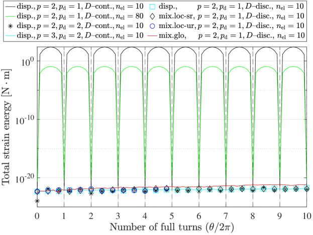
6.1 Rigid rotation of a stress-free rod: Objectivity test 1
We consider a quasi-static beam problem where the initial center axis is placed on the -plane and represents a quarter circle of radius . It has a square cross-section of dimension . We constrain one end of the beam, at which a rotation of angle (10 full turns) with respect to the -axis is prescribed. We prescribe the rotational motion by the two directors at the constrained end with their extensions not allowed. We incrementally apply the total rotation in 100 uniform increments (), and investigate the change of total strain energy. A St. Venant-Kirchhoff type isotropic hyperelastic material is considered with the Young’s modulus and the Poisson’s ratio . This example for testing the objectivity was proposed in Meier et al. [27, Sec. 11.1]. In Fig. 3, in cases of using the displacement-based beam formulation [disp.], and the continuous initial director field [–cont.] with , it is seen that the strain energy does not vanish (black and green curves), which represents the inability to represent the rigid body rotation (= non-objectivity). It is noticeable that the spurious strain energy vanishes in every full turn (= path-independence). It is also seen that the error decreases by increasing the number of elements (green curve). If we consider the continuous (exact) initial director field, we need at least quadratic NURBS basis functions in order to represent the rigid body rotation exactly, due to the circular initial geometry [9]. This can be seen in cases of using and 3 (black star and cyan curve) where the strain energy vanishes up to machine precision. In contrast, employing the discrete initial director field [–disc.] gives objectivity even with (cyan square, black diamond, blue circle, and red curve).
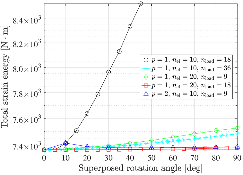
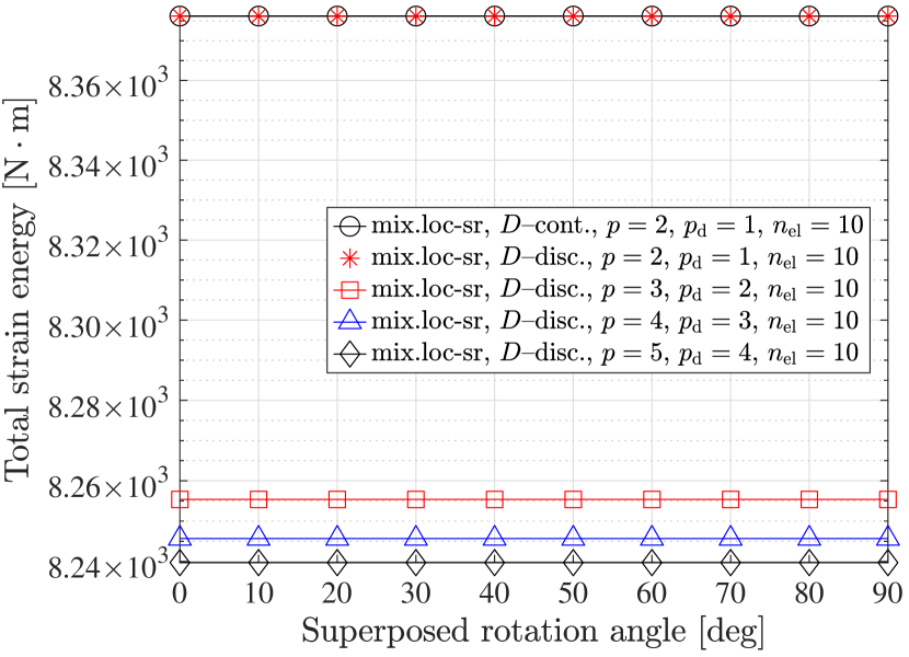
6.2 Rigid rotation of a bent rod: Objectivity test 2
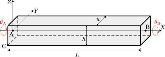
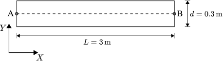
We investigate the invariance of non-vanishing strain under rigid body rotation superposed onto a deformed configuration in quasi-statics. This test was presented in Romero and Armero [33, Sec. 5.1]. We consider a straight beam in its initial (undeformed) configuration with the position vectors of center axis’ two end points A and B given by and , respectively, in a global Cartesian coordinate system. The application of external load is divided into two phases, whose boundary conditions are as follows:
-
•
First phase. The displacement of the end point B is prescribed by , with the directors at B free, and the cross-section at point A fixed. That is, we apply the boundary conditions
(165a) (165b) and (165c) -
•
Second phase. In order to investigate the objectivity, a series of nine rigid body rotations are quasi-statically superposed onto the deformed configuration after the first phase. We apply the boundary conditions
(166) and
(167) for , where
(168) with the axis of rotation
We consider a St. Venant-Kirchhoff type isotropic hyperelastic material with Young’s modulus and Poisson’s ratio , and a square cross-section of dimension . In this example, since the beam’s initial geometry is straight, the two approaches [–cont.] and [–disc.] yield the same initial director fields. In Fig. 4(a), it is seen that the beam formulation [] suffers from spurious strain energy in superposed rigid rotation, that is, it is non-objective. It is noticeable that the numerical error decreases by increasing number of load steps, in the second phase, where we use a uniform load increment. The reason for this is that the error in the finite element approximation of an incremental rotation should decrease, as the magnitude of rotation decreases. This can be seen, in the much lower spurious energy resulting from using doubled (cyan curve with star), compared with that of using (black curve with circle). This non-objectivity can be also alleviated by mesh refinement, a degree elevation (blue curve with triangle) or a larger number of elements (red curve with square). In contrast, the beam formulation with a direct finite element approximation of the director vectors [mix.loc-sr] exhibits no spurious strain energy in the second phase. In Fig. 4(b), both methods [–cont.] and [–disc.] give the same results and have constant strain energy under superposed rigid rotation (red star and black curve with circle). Fig. 4(b) also verifies the objectivity in higher degrees and (red, blue, and black curves).
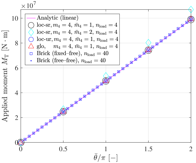
6.3 Straight beam under twisting moment
We consider a straight beam along the -axis that is subject to a prescribed twisting angle (), which is applied quasi-statically, about its center axis at both ends A and B in opposite directions. The beam has an initial length , and a rectangular cross-section of width and height , see Fig. 5. For the following cases of and , we verify that the present beam formulation can represent the correct torsional stiffness without additional global DOFs.
-
•
Case 1: , and ,
-
•
Case 2: , and .
A St. Venant-Kirchhoff type isotropic hyperelastic material with Young’s modulus and Poisson’s ratio is considered.
For comparison, we consider two different boundary conditions:
-
•
[free-free] Prescribe the rotation angles and . Note that, here, out-of-plane cross-sectional warping is allowed at both ends, A and B. For the brick solution, the -displacement is constrained at C in order to prevent a rigid-body translation.
-
•
[fixed-free] Fix the cross-section at A (), and prescribe the rotation angle at B. Note that we still allow for out-of-plane cross-sectional warping at the loaded end, B.
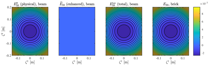
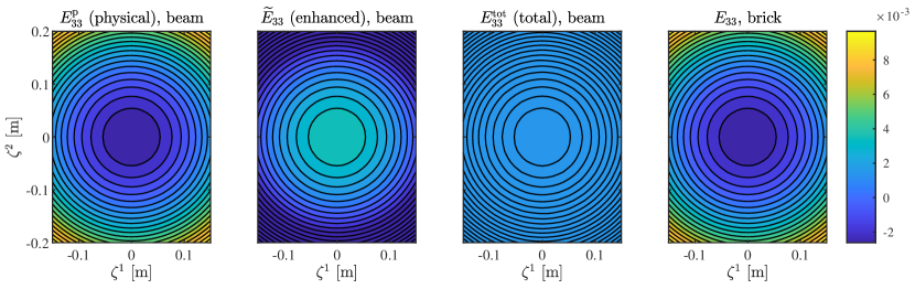
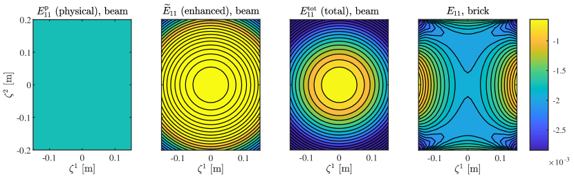
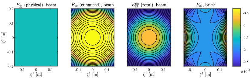
It should be noted that, in both cases of the boundary conditions, in-plane cross-sectional strains are not allowed at the ends. For beams, we use the [free-free] only, where the cross-sectional warping due to the enhanced strains is allowed at both ends. An application of boundary conditions to constrain the enhanced strain field remains future work. Figs. 6–11 compares the cross-sectional strains at the middle of the center axis () between the present beam and brick solutions for case 1 ( and ). Here, for the beam solution, we use [mix.loc-sr] with , , and . For the brick solution, we use deg.= and , and the [free-free] condition.
Observation 1.
In Fig. 6, it is seen that the enhanced strain vanishes. This implies that the quadratic polynomial basis in in the third row of Eq. (17) is sufficient to represent the axial normal strain. It has been also discussed in Wackerfuß and Gruttmann [41] that the enhancement of is not needed for a correct representation of the three-dimensional strain state. Accordingly, they presented a so called ‘E2–model’ which does not enrich the axial normal strain. This significantly reduces the number of internal DOFs for the enhanced strain field, which makes the formulation more efficient.
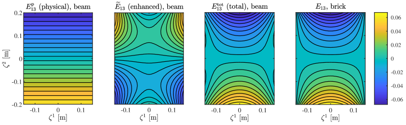
In Figs. 8 and 9, the physical transverse shear strains and are limited to linear distributions, since it has polynomial basis up to degree 1. It is noticeable that, by employing the enhanced strains, the total strains show excellent agreement with the brick solution, in both cases, and .
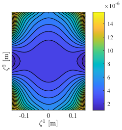
In Fig. 7, we show the beam solution using instead of , with all other parameters the same as in the result of Fig. 6. This aims at showing that losing the orthogonality between and can lead to significant error. Selecting the lower degree means that the basis may have quadratic terms in spite of the existing quadratic terms in . This eventually pollutes the physical strain field, which can be seen by the deviation of the resulting total strain from the brick solution.
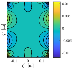
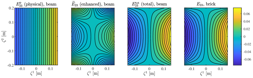
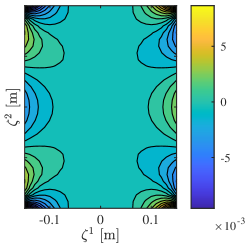
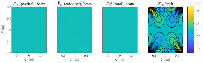
In Figs. 10 and 11, the physical in-plane cross-sectional strains and , respectively, have negative constant values, which represents a uniform transversal contraction of the cross-section. Although the enhanced strains improve the degree of approximation, they are limited to a quadratic distribution, due to the coupling with the axial normal strain by the non-zero Poisson’s ratio. Further, in case of the in-plane shear strain, the enhanced strain turns out not to be activated, as Fig. 12 shows. Further investigation on the selection of the basis and for improving the enhancement of in-plane cross-sectional strain remains future work.
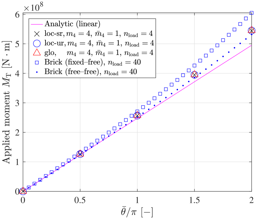
In Fig. 13, we compare the applied moment for a given prescribed rotation angle at the end () between the present beam element solution, the reference brick element solution, and the analytical solution in Eq. (214). In the first case ( and ), the beam solutions show excellent agreement with both analytic and brick element solutions. Overall, the mixed finite element formulation enables much larger load increments, compared to the displacement-based brick element formulation. In the second case ( and ), a nonlinear effect of increasing torsional stiffness along the prescribed rotation is clearly seen in both beam and brick solutions. In the latter range of the prescribed rotation, it is seen that the brick solution with the [fixed–free] boundary condition exhibits more rapidly increasing torsional stiffness compared to the solution using the [free-free] condition, due to the constrained out-of-plane warping at . It is remarkable that the beam and brick solutions under the [free–free] condition shows excellent agreement. In Table 1, we compare the total number of global and internal DOFs between beam and brick solutions. It is noticeable that the beam solutions use much smaller number of DOFs than the brick solution does, since the DOFs of the enhanced strain () can be element-wisely condensed out. In the beam formulation [mix.glo], the DOFs of the physical stress resultants () and physical strain () are considered in the global system of equations, whose number is much smaller than those of the local approaches for the same number of elements, due to the higher-order continuity of B-spline basis functions, see Remark 5.1.
| Beam [mix.loc-sr] | Beam [mix.loc-ur] | Beam [mix.glo] | Brick | |
| Degree of basis | , | , | ||
| #elements | 40 | 40 | 40 | |
| #DOFs () | 381 | 381 | 387 | 42,081 |
| #DOFs () | 814 | 1200 | 630 | – |
| #DOFs () | 814 | 1200 | 630 | – |
| #DOFs () | 1,080 | 1,080 | 1,080 | – |
| #global DOFs | 381 | 381 | 1,647 | 42,081 |
| #internal DOFs | 2,708 | 3,480 | 1,080 | – |
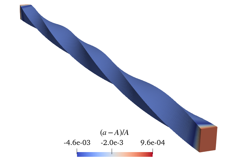
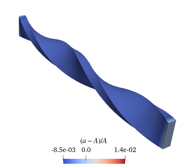
Figs. 14 and 15 compare the deformed configurations between the beam and brick solutions for the two different dimensions of the initial cross-section. It is noticeable that the same level of decrease of the cross-sectional area is observed in the beam and brick solutions. In the brick solution, it is seen that the cross-sectional area slightly increases at both ends, due to the out-of-plane warping. This is not explicitly shown in the beam solution, since we calculate the cross-sectional area using only two directors and , which can only represent a planar cross-section deformations.

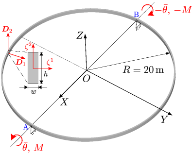
6.4 Twisting of an elastic ring
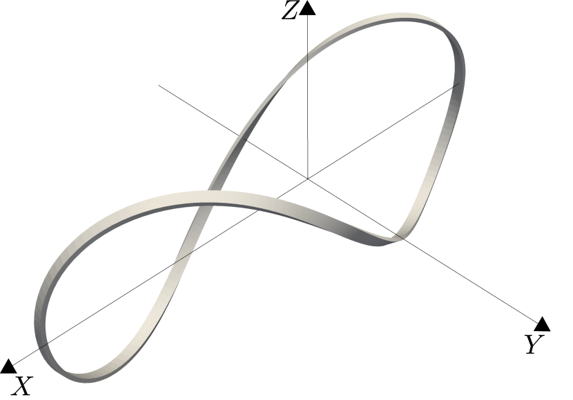
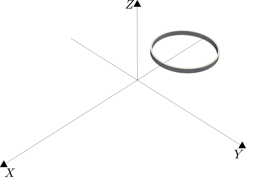
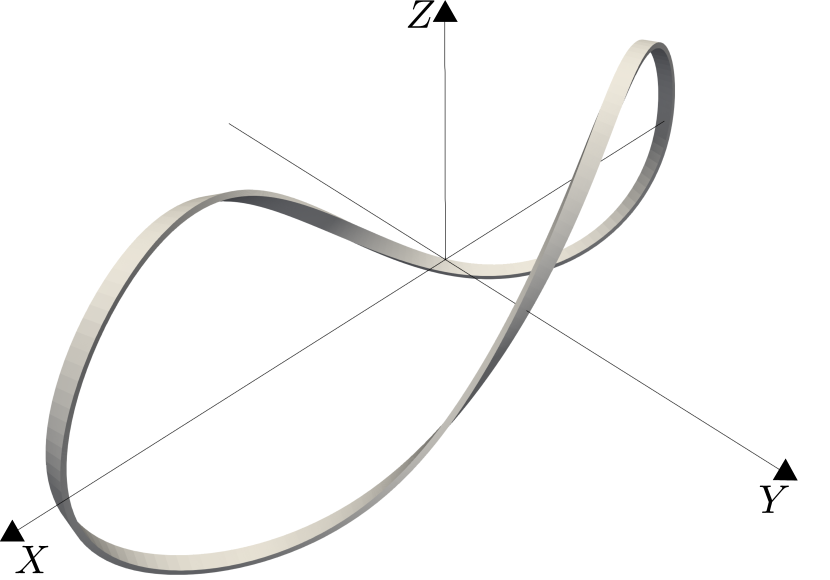
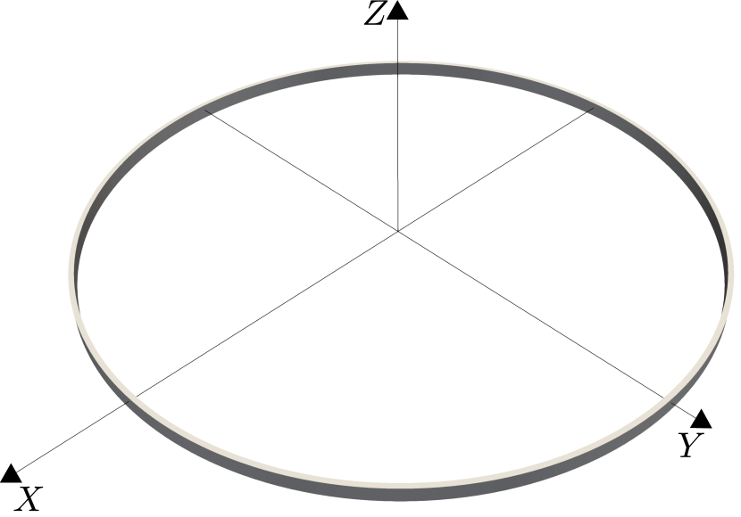
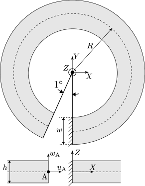
We consider a closed circular ring twisted by a prescribed rotation. Fig. 16 shows the undeformed configuration and boundary conditions. The initial ring has a radius , and a rectangular cross-section having width and height . We prescribe a rotation of the cross-sections at the material points of initial coordinates (point A) and (point B) by the angle with respect to the -axis in opposite directions. We apply the prescribed rotation angle [rad] in total, such that the configuration finally goes back to the initial (undeformed) one, if no impenetrability condition is imposed, see Fig. 17 for the deformed configurations at different values of . For , the ring is folded into a smaller circular ring. Without axial strain, the radius of the deformed ring is , which was first theoretically investigated by Goto et al. [17]. With axial strain, the deformed configuration is still a folded ring, but has a different radius such that , where denotes the current total length. In the present paper, this example aims at the following:
-
•
Verify the capability of the present beam formulation to follow the correct equilibrium path of the deformation by correcting the torsional stiffness through the enrichment of higher-order cross-sectional strains,
-
•
Investigate the effect of axial strain coupled with bending strain in the present beam formulation. The coupled axial strain changes the total length , and subsequently the radius of the deformed ring becomes at . This additional strain should quadratically decrease with increasing slenderness ratio [8, Section 6.2]. In order to show this, we consider the following two different cases with cross-sectional dimensions:
-
–
Case 1: , and ,
-
–
Case 2: , and .
Note that, here, we always have a ratio , which is known to produce a deformed configuration of a smaller ring by the prescribe rotation [17].
-
–
-
•
Verify the path-independence of the present beam formulation.
A St. Venant-Kirchhoff type isotropic hyperelastic material is considered, with Young’s modulus , and Poisson’s ratio . In order to account for the decreased torsional stiffness due to the cross-sectional warping, we employ the following approaches:
-
•
In the beam formulation [], we correct the torsional stiffness by replacing the polar moment of inertia with , see Appendix C.1. Note that is much smaller than the polar moment of inertia, . For example, in case of and , we have and , which gives the polar moment of inertia much larger than the corrected value . This approach refers to Romero [32], Meier et al. [26], and references therein.
-
•
For the present beam formulation, instead of directly adjusting the cross-sectional parameters, we enrich the polynomial basis functions up to degree for the transverse shear strains and , and for the in-plane strains , , and . Note that the axial normal strain component is not enriched, due to the observation in Remark 1.
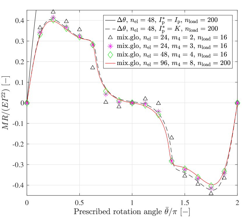
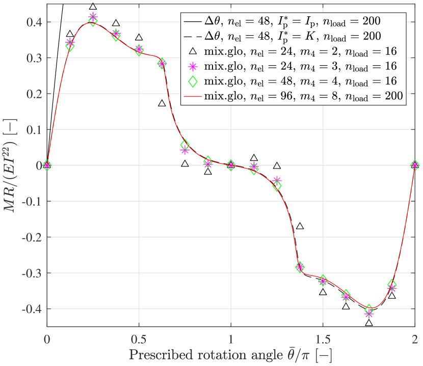
In Fig. 18, we compare the equilibrium paths from using the formulation [] and the present one [mix.glo]. The black solid curves represent the result from [] using the corrected torsional stiffness with . Note that, without this correction (i.e., with ), the torsional stiffness is significantly overestimated, see the much larger initial slope of the black solid curves compared to the others. This eventually leads to the divergence in the equilibrium iteration under the prescribed rotation. The black dashed curves represent the equilibrium paths with the corrected torsional stiffness. In the results from the present beam formulation [mix.glo], we first enrich the transverse normal strain components and by the maximum degree of basis in order to obtain the correct bending stiffness due to the nonzero Poisson’s ratio. Then, as we increase the maximum degree of enriched basis for the transverse shear strain , the equilibrium path approaches the result from using (red curve).
We have an analytical solution of the deformed center axis such that it becomes a folded circular ring of radius at [17]. However, it turns out that additional axial compression can be induced by bending [8, Sec.6.2.1]. In order to illustrate this, in Fig. 19, we compare the approximated total length of the center axis at between the results from the formulations [] and [mix.glo]. It is noticeable that, in the present beam solution (red curve), the beam is axially compressed, in contrast to the result from using []. Further, it is seen that the amount of compressive strain decreases by times, with increasing the slenderness ratio by times from Case 1 to Case 2. This means that as expected, the decrease of the coupled axial strain is in quadratic order with respect to the slenderness ratio. Based on this, we introduce a corrected reference solution for the deformed center axis at , such that it is still a folded circular ring, but with radius , where the (approximated) total length is given by an overkill solution from using the present beam formulation, [mix.glo] with . From this, we can define a relative -difference of the center axis displacement field, as
| (169) |
where the reference center of the circle is given by .
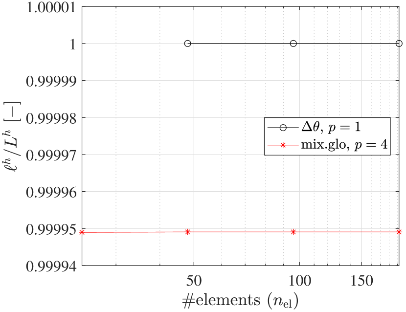
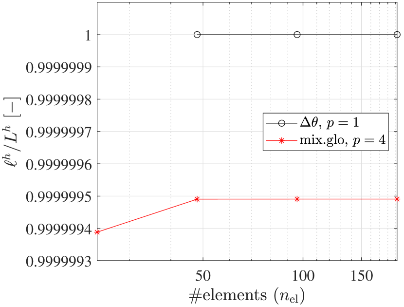
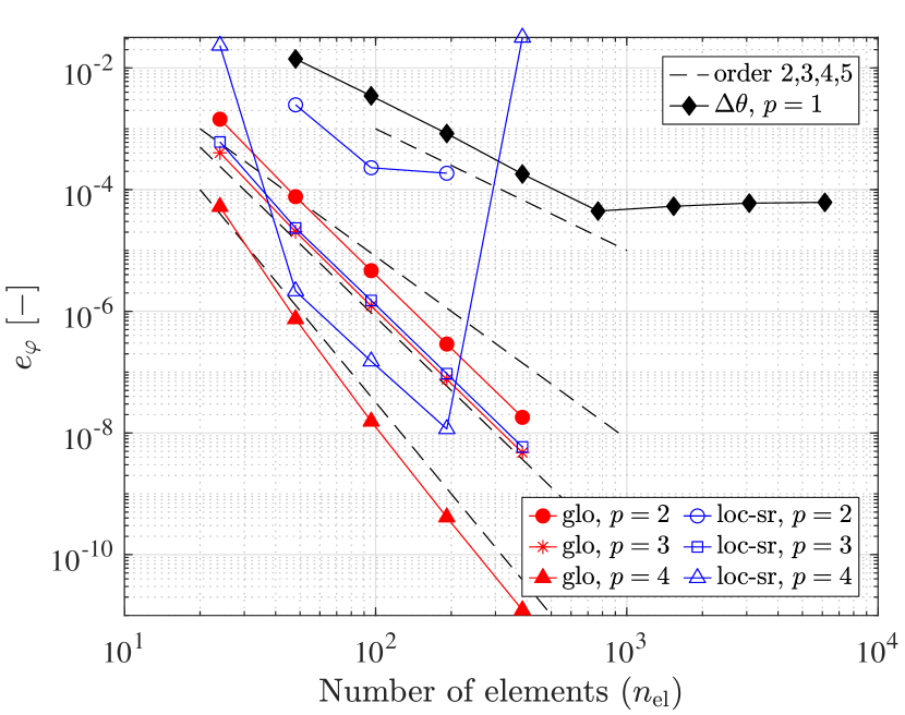
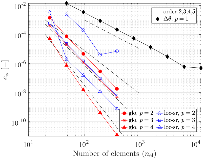
Fig. 20 shows the convergence of the relative differences from two different beam formulations, with the degree of basis , and the present one [mix.glo] with degree of basis . It is seen that in both cases 1 and 2, the present beam solution from using [mix.glo] converges toward the reference one (a folded circular ring with radius ), with increasing number of elements. In contrast, the beam formulation yields a different solution, which deviates from the reference one. This deviation is due to the inability to represent the axial strain coupled with bending, and it should decrease quadratically with increasing slenderness ratio. It is also noticeable that the results from [mix.glo] exhibit optimal convergence rates () or sometimes even faster, which can be clearly seen in both cases. In the results from using the beam formulation [mix.loc-sr], deteriorated convergence is observed due to numerical instability, except for the results from using . In Table 2, we compared the total number of load steps and equilibrium iterations between [mix.glo] and [mix.loc-sr]. The present formulation [mix.glo] shows stability in all cases.
In Goto et al. [17], it is shown that the deformed smaller ring at can stay without any external load. Further, due to the symmetry, the configuration should go back to the initial (undeformed) one at by either loading or unloading from the smaller ring at . That is, if a formulation is path-independent, the applied moment should vanish at both and . Figs. 21(a) and 21(b) plot the convergence of the moments at and , respectively, with increasing number of elements. It is seen that, for the formulation [], the moments do not vanish, which implies that the formulation suffers from path-dependence. Note that this error decreases in quadratic order, which is consistent with the convergence rate of the displacement field in Fig. 20. In contrast, from using the present beam formulation, the moments vanish up to machine precision for any number of elements.
The next two examples deal with nonlinear transient dynamics to verify the present time-stepping scheme.
6.5 Dynamics of a flying beam
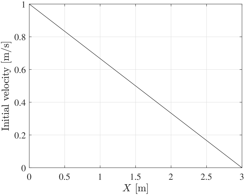
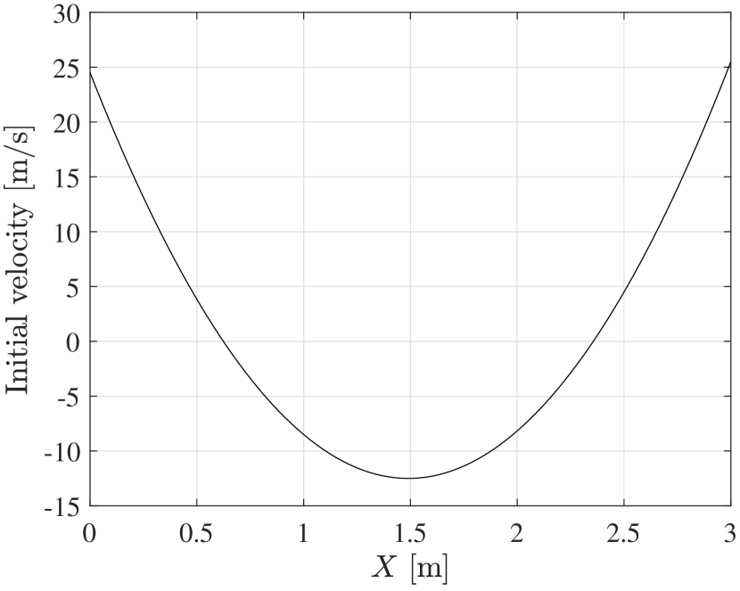
We consider an initially straight beam of length which has a square cross-section of dimension , see Fig. 22. A St. Venant-Kirchhoff type hyperelastic material with Young’s modulus and Poisson’s ratio is considered. The initial mass density is . We apply an initial velocity condition in – and – directions along the initial center axis, as
| (170a) | ||||
| (170b) | ||||
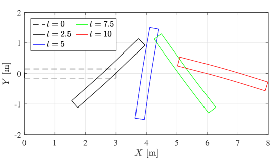
respectively, with and , see also Fig. 23. The directors are assumed initially stationary, which means that all the material points in each cross-section have the same initial velocity. The initial velocity component in Eq. (170a) leads to a translation in – direction. In Eq. (170b), the quadratic – directional velocity by the first term leads to the bending and transversal shear strains in the – plane, as well as the transverse normal strain due to the non-zero Poisson’s ratio. The second term in Eq. (170b) is introduced to have a rotational motion in the – plane. Therefore, the total linear and angular momentum vectors may have non-zero components in –, and – directions, respectively. Fig. 24 shows the deformed configurations at selected time instants.
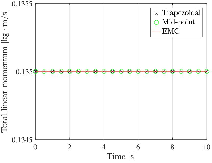
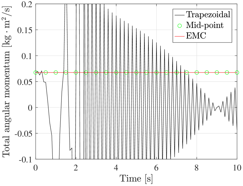
In Fig. 25, we investigate the conservation of energy and momentum. It is seen that the standard trapezoidal rule conserves the linear momentum, but neither the angular momentum nor the total energy. For the given time step size , the total energy blows-up. The total angular momentum initially has non-zero value due to the initial velocity condition, and is maintained by both the standard mid-point rule and the present EMC schemes. Initially, the total energy only has a kinetic part, and it is exactly conserved by the present EMC scheme. This implies the symmetry between the strain energy () and the kinetic energy (). In contrast, when using the mid-point rule, the total energy is not conserved, but blows-up. Here, for all the beam solutions, we use [mix.glo] with , , and , , with no enrichment for .
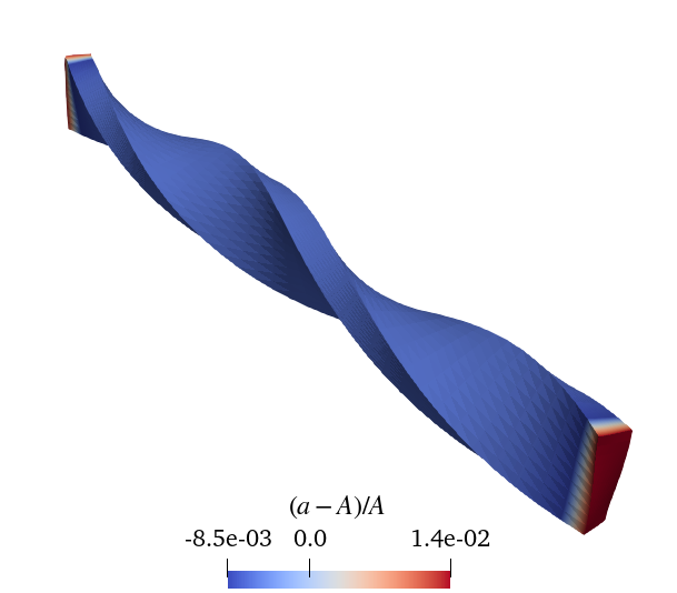
6.6 Slotted ring with a rectangular cross-section
An initially circular ring of radius with a slot of angle is considered. It has a rectangular cross-section of height and width , see Fig. 26. One end is fixed, where no cross-sectional deformation is allowed, and a distributed force is applied in -direction on the other end (cross-section at point A). In this example, we investigate two different types of loading:
-
•
Case 1 (elastostatics): A quasi-statically applied surface traction (force per unit undeformed area), , where ,
-
•
Case 2 (elastodynamics): A (piece-wise linearly) time-dependent surface traction, , where (force per unit undeformed area) is given by
| (173) |
Here, , denotes a unit time, and denotes the terminal time.
6.6.1 Case 1: Comparison with the brick element solution
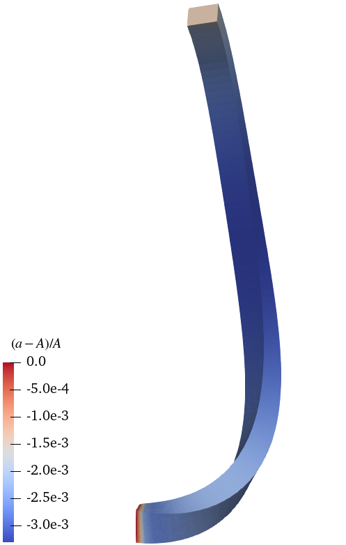
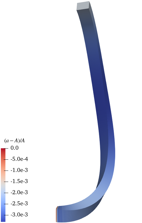
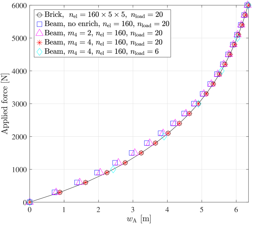
We consider a Neo-Hookean type isotropic hyperelastic material with Young’s modulus , and Poisson’s ratio . For the given load, the ring undergoes a large deformation with torsion-induced cross-sectional warping. Here, we verify the corrected torsional stiffness from using the present EAS method. In Fig. 27, we compare the deformed configurations between the present beam and the brick element solutions, where it is seen that the cross-section contracts due to the positive Poisson’s ratio, except for the fixed end. It is seen that the change of cross-sectional area can be properly represented by only two directors in the present beam formulation.
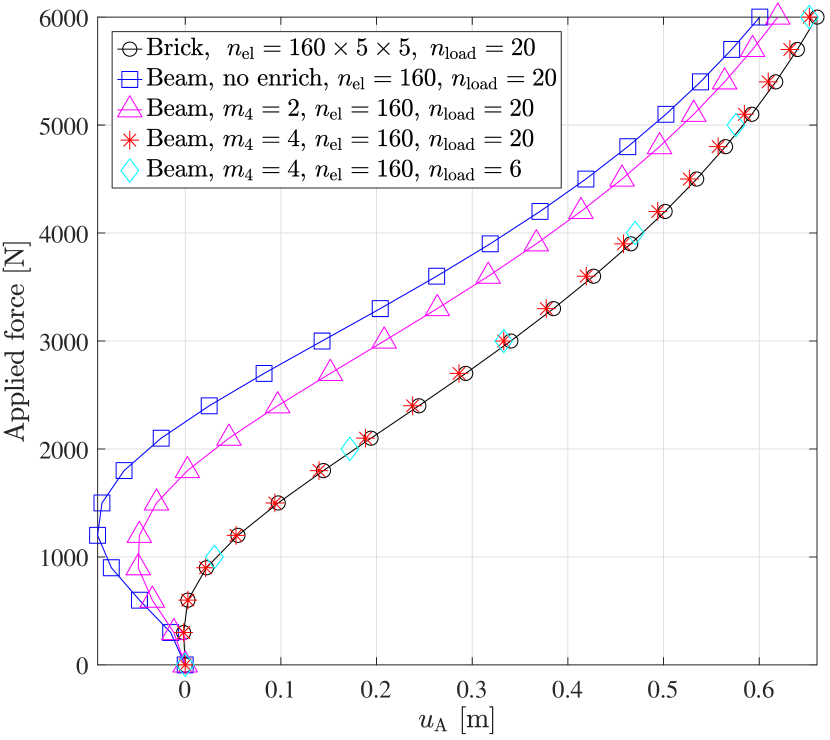
Figs. 28(a) and 28(b) show the – and –displacements of the ring at point A, which are denoted by and , respectively. In the beam formulation, we compare different degrees of the polynomial basis for the transverse shear strains, and . Note that we also use , and the axial normal strain has not been enriched. It is seen that without the enrichment of the transverse shear strain, the beam solution (blue curve) deviates signifcantly from the brick solution (black curve). It is noticeable that with increasing degree , the solution approaches the brick solution (magenta and red marks). Further, a much larger load step is allowed in the present beam formulation, compared to the displacement-based brick formulation, which can be seen by the results of the beam element using 6 uniform load increments (cyan mark).
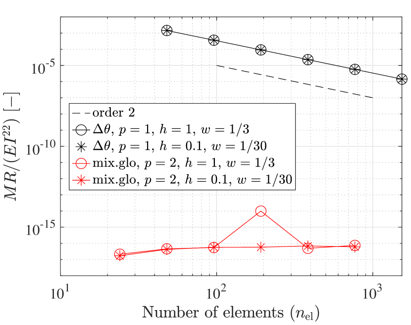
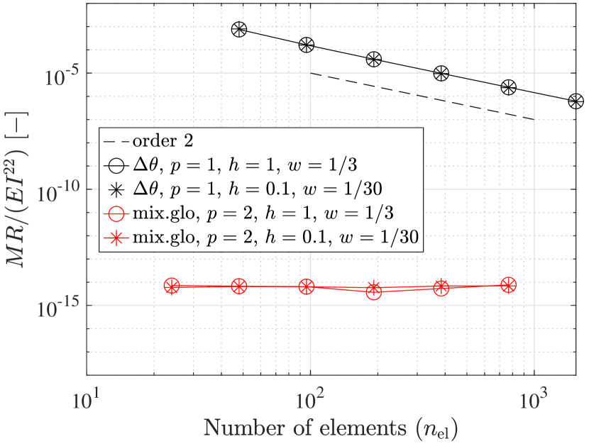
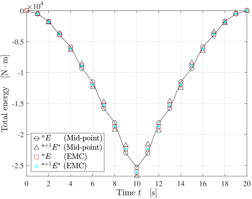
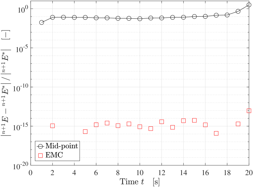
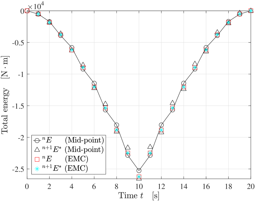
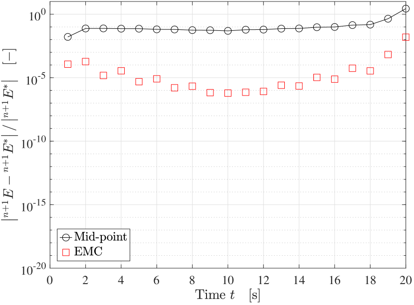
6.6.2 Case 2: Verification of the consistency in the EMC scheme
In the second case, we investigate a transient dynamic response of the slotted ring, under the time-dependent load given by Eq. (173). The total simulation time is . Figs. 29 and 30 investigate whether a time-stepping scheme satisfies the following identity
| (174) |
which is recalled from Eq. (213). For constitutive laws, we consider two different models, St. Venant-Kirchhoff (linear) and Neo-Hookean (nonlinear) types, with the same values of the parameters and as in the case 1. The initial mass density is . From using the standard mid-point rule, it is seen that the total energy deviates from for both linear and nonlinear constitutive laws. In contrast, the EMC scheme satisfies the identity exactly (up to machine precision) for the linear constitutive law, see Fig. 29(b). For the nonlinear constitutive law, the EMC scheme has also lost the consistency, but the relative difference is much smaller than that from the mid-point rule, see Fig. 30(b).
7 Conclusions
We present a stable and efficient implicit isogeometric finite element method for geometrically and materially nonlinear beams in transient dynamics. The superior numerical stability of the developed method comes from the following aspects:
-
•
Objectivity and path-independence of the isogeoemtric finite element formulation that directly approximates the director field, which turns out to hold for any degree , which is verified in several numerical examples. This formulation is based on the approximation of the initial director field, which is, in the present paper, denoted by [-disc.].
-
•
An energy–momentum consistent (EMC) time-stepping scheme, which gives exact energy conservation property for linear constitutive laws.
-
•
Employing the independent DOFs for the stress resultants in the mixed finite element formulation based on the Hu-Washizu variational principle alleviates the overestimation of the internal force, which improves the stability of the equilibrium iteration for larger time (load) steps in the Newton-Raphson method.
-
•
In the isogeometric approach, we have observed numerical instabilities of the local approach [mix.loc-sr] in some cases. The present global approach [mix.glo] shows numerical stability in all those cases. Further, compared to the local approach, the present global approach requires much less degrees-of-freedom for the physical stress resultants and strains due to the higher-order continuity of the B-spline basis functions.
Further, the developed method provides superior computational efficiency, compared to brick element formulations, due to the following aspects:
-
•
The present 9-DOF formulation with extensible (unconstrained) directors allows for an efficient representation of a constant in-plane cross-sectional strain, e.g., the change of cross-sectional area.
-
•
The higher order cross-sectional strains like torsion-induced warping have been further enriched by an EAS method. Due to the allowed inter-element discontinuity in the enhanced strain field, one can eliminate those additional DOFs from the global system of linear equations.
One can extend the present work in the following aspects:
-
•
In the inertia terms, we have considered the cross-sectional deformation only up to the constant strains, represented by two extensible directors.
-
•
We have limited our scope of investigation to convex-shaped cross-sections like a rectangular one.
-
•
The present EAS method corrects torsional stiffness very effectively; however, it is seen that the enrichment of in-plane cross-sectional strains is limited.
Acknowledgements M.-J. Choi was supported by the Alexander von Humboldt Foundation (postdoctoral research fellowship) in Germany, and the Deutsche Forschungsgemeinschaft (DFG, German Research Foundation) - Project number 523829370.
Author contributions Myung-Jin Choi: Writing - review & editing, writing - original draft, investigation, conceptualization, methodology, software, validation, visualization, formal analysis, data curation, resources. Sven Klinkel: Writing - review & editing, investigation, conceptualization, resources, supervision. Simon Klarmann: Writing - review & editing, investigation, conceptualization. Roger A. Sauer: Writing - review & editing, investigation, conceptualization, supervision.
Declarations
The authors declare that they have no conflict of interest.
Appendix A Beam formulation
A.1 Objectivity of the geometric strain in continuous form
The invariance of the beam strain components under a superposed rigid body motion can be analytically verified. We superpose an arbitrary constant rigid body rotation and translation to the current configuration , as [11]
| (175a) | ||||
| (175b) | ||||
where denotes a three-dimensional rotation group, defined as
| (176) |
By inserting Eqs. (175a) and (175b) into Eqs. (18a)–(18f), and using , , and , we have
| (177) |
A.2 Objectivity of the geometric strain in discrete form
We investigate the invariance of the strain measures approximated by Eqs. (116) and (117) under superposed rigid body translation and rotation. We superpose an arbitrary constant rigid body rotation and translation to the current control coefficients and , as
| (178a) | ||||
| and | ||||
| (178b) | ||||
, where we utilize the partition of unity property of the NURBS basis functions. Therefore, substituting Eqs. (178a) and (178b) into Eqs. (18a)–(18f), and using , , and , the beam strain at the superposed configuration , we have
| (179) |
which represents the frame-invariance (objectivity) of the approximated beam strain.
A.3 Construction of warping basis functions
Here we discuss the determination of the polynomial basis , , , and in Eq. (33). Note that this is a generalization of the formulation of Wackerfuß and Gruttmann [40] in order to account for the higher order strains in Eq. (10) from the beam kinematics.
A.3.1 Orthogonality condition
Here we construct a complete set of polynomials up to degree that are orthogonal to an arbitrary polynomial of degree . We first introduce the following arrays [41]
| (180) |
with , , where denotes the maximum degree, and we define
Here, denotes the set of positive integers, and the number of elements in is . Further, we introduce a modified polynomial basis
| (181) |
where we define, for each ,
| (182) |
with the coefficients ,
| (183) |
such that the following orthogonality to arbitrary polynomials up to degree is satisfied:
| (184) |
where whose number of elements is . Equation (182) can be rewritten in the compact form
| (185) |
with and . Substituting Eq. (182) into Eq. (184), we obtain the following system of linear equations to determine for each :
| (186) |
where the system matrix is given by
| (187) |
Remark A.1:
Since is invertible, the coefficients for each can be uniquely determined by solving Eq. (186). It should be noted that Eq. (186) depends solely on the cross-section’s initial shape and dimension. Therefore, this process to contruct a complete set of polynomial basis functions of maximum degree , can be done in pre-processing. For a given (fixed) value of , the total time for determining the whole coefficients , is linearly proportional to the number of elements in , , i.e., the time complexity of constructing is .
A.3.2 Polynomial basis for enhanced strains
Here, we show the construction of polynomial basis , , , and in Eq. (33), based on the method in Section A.3.1. The enhanced basis can be expressed by
| (188) |
where denotes the maximum degree of the polynomial, and denotes the maximum degree in the corresponding compatible strain component, i.e., from Eq. (17), we have , , and . We first show that the orthogonality condition in Eq. (24) can be simplified to the form of Eq. (184). Since the orthogonality condition in Eq. (24) should hold for all , we obtain
| (189) |
where , such that . Further, we make the following assumptions in the evaluation of the orthogonality condition in Eq. (189):
-
•
has the same polynomial order in and as the conjugate strain component in Eq. (25).
-
•
, which holds exactly only for initially straight beams or linear finite elements, see Remark 2.1. This makes the orthogonality condition solely depend on the cross-section’s initial shape.
Then, we obtain the following orthogonality condition: For each , we have
| (190) |
which has the same form as Eq. (184). Subsequently, for in each , , the unknown coefficients in can be determined from solving Eq. (A.1), with replaced by . Here, denotes the number of elements in the row array , and it is obtained by
| (191) |
Therefore, from Remark A.1, the time complexity to construct is , .
Appendix B Time-stepping scheme
B.1 Verification of the energy–momentum conservation for continuous time
Here we verify that energy–momentum conservation laws can be deduced from Eq. (64) under appropriate boundary conditions.
B.1.1 Total linear momentum
Let with a constant vector , which describes a superposed rigid body translation. Here we assume no displacement boundary conditions, i.e., , so that . Then, the internal virtual work vanishes, and from Eq. (64a), we obtain
| (192) |
with the time-dependent total external force,
| (193) |
Therefore, without any displacement boundary conditions, we have the balance of total linear momentum
| (194) |
This implies that the total linear momentum is conserved if no external force and displacement boundary condition are applied.
B.1.2 Total angular momentum
Let with a constant vector , which represents a superposed (infinitesimal) rigid body rotation, and represents the rotation axis vector. Here, we also assume no displacement boundary conditions, i.e., , so that . Then, the internal virtual work vanishes, and from Eq. (64a), we obtain
| (195) |
with the total external moment defined by
| (196) |
Therefore, without any displacement boundary conditions, we have the balance of total angular momentum
| (197) |
B.1.3 Total energy
We define the total energy at an equilibrium solution of Eq. (64), by
| (198) |
where the internal energy can be evaluated, from Eq. (34), by
| (199) |
We choose , and have the compatibility condition from Eq. (65). Then from Eq. (64a), we obtain
| (200) |
This means that the total energy is conserved unless the external load has an explicit dependence on time. That is, for a conservative system, we have
| (201) |
where the total energy is
| (202) |
B.2 Verification of the energy–momentum conservation in discrete-time intervals
We show that the time-stepping scheme in Eq. (73) preserves the conservation properties of the continuous form in Section B.1.
B.2.1 Total linear momentum
Let with a constant vector . Here we assume no displacement boundary condition, i.e., , so that . Then, we obtain the discrete form of the linear momentum balance from Eq. (73a), as
| (203) |
which is consistent with Eq. (192). Therefore, the total linear momentum is conserved, if no external force and displacement boundary conditions are applied.
B.2.2 Total angular momentum
We choose
| (204) |
with a constant vector , and assume no displacement boundary conditions, i.e., , so that . Then, from Eq. (73a), we obtain
| (205) |
which is consistent with Eq. (197). Therefore, the angular momentum is conserved if no external loads and boundary conditions are applied. Note that this holds for both the conventional mid-point rule and the present EMC scheme.
B.2.3 Total energy
We choose . Then, from Eq. (73a), using Eq. (71), we have
| (206) |
Further, due to the linearity of the operator with respect to , we can obtain
| (207) |
Then, from Eq. (38a), we have
| (208) |
By choosing and in Eqs. (73c) and (73d), respectively, and combining the resulting equations, we obtain the identity,
| (209) |
Evaluating Eq. (73b) at time and with , we have
| (210a) | ||||
| (210b) | ||||
respectively. Eqs. (210a) and (210b) imply that Eqs. (208) and (209) are the same, so that we obtain the identity
| (211) |
Substituting Eqs. (B.2.3) and (B.2.3) into Eq. (73a), we have
| (212) |
This implies the following:
-
•
If the applied load is (piece-wise) linearly proportional to time, we obtain the following identity
(213) where we define
with
and
-
•
If the external load has no explicit time-dependence, the total energy is conserved, i.e., .
Appendix C Numerical examples
C.1 An analytical solution for a pure torsion problem
We consider a pure torsion of a straight bar of length , and a shear modulus . In the isotropic linear elasticity, the torsional angle (radians) of the bar under a twisting moment can be expressed by [4, page 350]
| (214) |
where is a factor which depends on the cross-sectional shape and dimensions. For a circular cross-section, the cross-section remains plane under the moment load, and is equal to the polar moment of inertia, . For other cross-sections, the cross-section warps, and is less than . For a (solid) rectangular cross-section of dimensions and (), we have a solution for in Budynas and Sadegh [4, page 366, Table 10.7],
| (215) |
obtained from a truncation of an infinite series solution of the St. Venant torsion problem, which can be found in Timoshenko and Goodier [39, page 288]. From Eq. (214), represents the torsional stiffness of the bar. Note that Eq. (215) is based on the assumptions [4, page 349]: (i) The bar is straight, (ii) the material is homogeneous, isotropic, and linear elastic, (iii) the deformation is purely torsional under equal and opposite twisting moments at the ends.
C.2 Total number of load steps in example 4
Here we present total number of load steps and iterations in the results of Fig. 20. For the formulation [], we use in total 200 and 2,000 load steps with uniform increments in cases 1 and 2, respectively. Table 2 shows the total number of load steps and iterations in the results from using [mix.glo] and [mix.loc-sr]. We have observed that, using [mix.loc-sr] with and , the ring does not deform into a smaller one, and the equilibrium iteration eventually diverges.
| Case 1: , | Case 2: , | |||||||||||
| [mix.loc-sr] | [mix.glo] | [mix.loc-sr] | [mix.glo] | |||||||||
| 2 | 24 | 96 | - | 16 | 105 | 96 | - | 16 | 103 | |||
| 48 | 96 | 641 | 16 | 103 | 96 | 523 | 16 | 101 | ||||
| 96 | 96 | 673 | 16 | 103 | 192 | 973 | 16 | 100 | ||||
| 192 | 16 | 224 | 16 | 102 | 16 | 183 | 16 | 100 | ||||
| 384 | 384 | 20 | 161 | 16 | 208 | 16 | 100 | |||||
| 3 | 24 | 16 | 105 | 16 | 105 | 16 | 105 | 16 | 103 | |||
| 48 | 16 | 104 | 16 | 103 | 16 | 103 | 16 | 101 | ||||
| 96 | 16 | 104 | 16 | 103 | 16 | 103 | 16 | 100 | ||||
| 192 | 16 | 116 | 16 | 114 | 16 | 103 | 16 | 100 | ||||
| 384 | 16 | 144 | 20 | 248 | 16 | 103 | 16 | 100 | ||||
| 4 | 24 | 16 | 150 | 16 | 105 | 16 | 109 | 16 | 103 | |||
| 48 | 16 | 140 | 16 | 103 | 16 | 104 | 16 | 101 | ||||
| 96 | 16 | 141 | 16 | 103 | 16 | 103 | 16 | 100 | ||||
| 192 | 64 | 480 | 16 | 157 | 16 | 104 | 16 | 100 | ||||
| 384 | 64 | 445 | 36 | 253 | 16 | 104 | 16 | 100 | ||||
References
- \bibcommenthead
- Betsch and Janz [2016] Betsch, P. and A. Janz. 2016. An energy–momentum consistent method for transient simulations with mixed finite elements developed in the framework of geometrically exact shells. International Journal for Numerical Methods in Engineering 108(5): 423–455 .
- Betsch and Steinmann [2002] Betsch, P. and P. Steinmann. 2002. Frame-indifferent beam finite elements based upon the geometrically exact beam theory. International Journal for Numerical Methods in Engineering 54(12): 1775–1788 .
- Büchter et al. [1994] Büchter, N., E. Ramm, and D. Roehl. 1994. Three-dimensional extension of non-linear shell formulation based on the enhanced assumed strain concept. International journal for numerical methods in engineering 37(15): 2551–2568 .
- Budynas and Sadegh [2020] Budynas, R. and A. Sadegh. 2020. Roark’s formulas for stress and strain. McGraw-Hill Education.
- Casquero and Golestanian [2022] Casquero, H. and M. Golestanian. 2022. Removing membrane locking in quadratic NURBS-based discretizations of linear plane Kirchhoff rods: CAS elements. Computer Methods in Applied Mechanics and Engineering 399: 115354 .
- Choi and Cho [2019] Choi, M.J. and S. Cho. 2019. Isogeometric configuration design sensitivity analysis of geometrically exact shear-deformable beam structures. Computer Methods in Applied Mechanics and Engineering 351: 153–183 .
- Choi et al. [2022] Choi, M.J., S. Klinkel, and R.A. Sauer. 2022. An isogeometric finite element formulation for frictionless contact of Cosserat rods with unconstrained directors. Computational Mechanics 70(6): 1107–1144 .
- Choi et al. [2021] Choi, M.J., R.A. Sauer, and S. Klinkel. 2021. An isogeometric finite element formulation for geometrically exact Timoshenko beams with extensible directors. Computer Methods in Applied Mechanics and Engineering 385: 113993 .
- Choi et al. [2023] Choi, M.J., R.A. Sauer, and S. Klinkel. 2023. A selectively reduced degree basis for efficient mixed nonlinear isogeometric beam formulations with extensible directors. Computer Methods in Applied Mechanics and Engineering 417: 116387 .
- Coda [2009] Coda, H.B. 2009. A solid-like FEM for geometrically non-linear 3D frames. Computer methods in applied mechanics and engineering 198(47-48): 3712–3722 .
- Crisfield and Jelenić [1999] Crisfield, M. and G. Jelenić. 1999. Objectivity of strain measures in the geometrically exact three-dimensional beam theory and its finite-element implementation. Proceedings of the Royal Society of London. Series A: Mathematical, Physical and Engineering Sciences 455(1983): 1125–1147 .
- Dornisch et al. [2013] Dornisch, W., S. Klinkel, and B. Simeon. 2013. Isogeometric Reissner–Mindlin shell analysis with exactly calculated director vectors. Computer Methods in Applied Mechanics and Engineering 253: 491–504 .
- Durville [2012] Durville, D. 2012. Contact-friction modeling within elastic beam assemblies: an application to knot tightening. Computational Mechanics 49(6): 687–707 .
- Farin and Hansford [2000] Farin, G. and D. Hansford. 2000. The essentials of CAGD. AK Peters/CRC Press.
- Frischkorn and Reese [2013] Frischkorn, J. and S. Reese. 2013. A solid-beam finite element and non-linear constitutive modelling. Computer Methods in Applied Mechanics and Engineering 265: 195–212 .
- Gonzalez [2000] Gonzalez, O. 2000. Exact energy and momentum conserving algorithms for general models in nonlinear elasticity. Computer Methods in Applied Mechanics and Engineering 190(13-14): 1763–1783 .
- Goto et al. [1992] Goto, Y., Y. Watanabe, T. Kasugai, and M. Obata. 1992. Elastic buckling phenomenon applicable to deployable rings. International journal of solids and structures 29(7): 893–909 .
- Gruttmann et al. [2000] Gruttmann, F., R. Sauer, and W. Wagner. 2000. Theory and numerics of three-dimensional beams with elastoplastic material behaviour. International Journal for Numerical Methods in Engineering 48(12): 1675–1702 .
- Hughes et al. [2005] Hughes, T., J. Cottrell, and Y. Bazilevs. 2005. Isogeometric analysis: CAD, finite elements, NURBS, exact geometry and mesh refinement. Computer Methods in Applied Mechanics and Engineering 194(39-41): 4135–4195 .
- Jelenić and Crisfield [1999] Jelenić, G. and M. Crisfield. 1999. Geometrically exact 3D beam theory: implementation of a strain-invariant finite element for statics and dynamics. Computer methods in applied mechanics and engineering 171(1-2): 141–171 .
- Kikis and Klinkel [2022] Kikis, G. and S. Klinkel. 2022. Two-field formulations for isogeometric Reissner–Mindlin plates and shells with global and local condensation. Computational Mechanics: 1–21 .
- Klarmann et al. [2022] Klarmann, S., J. Wackerfuß, and S. Klinkel. 2022. Coupling 2D continuum and beam elements: a mixed formulation for avoiding spurious stresses. Computational Mechanics 70(6): 1145–1166 .
- Klinkel and Govindjee [2003] Klinkel, S. and S. Govindjee. 2003. Anisotropic bending-torsion coupling for warping in a non-linear beam. Computational Mechanics 31(1): 78–87 .
- Klinkel et al. [2006] Klinkel, S., F. Gruttmann, and W. Wagner. 2006. A robust non-linear solid shell element based on a mixed variational formulation. Computer Methods in Applied Mechanics and Engineering 195(1-3): 179–201 .
- Lanczos [2012] Lanczos, C. 2012. The variational principles of mechanics. Courier Corporation.
- Meier et al. [2014] Meier, C., A. Popp, and W. Wall. 2014. An objective 3D large deformation finite element formulation for geometrically exact curved Kirchhoff rods. Computer Methods in Applied Mechanics and Engineering 278: 445–478 .
- Meier et al. [2019] Meier, C., A. Popp, and W. Wall. 2019. Geometrically exact finite element formulations for slender beams: Kirchhoff–Love theory versus Simo–Reissner theory. Archives of Computational Methods in Engineering 26(1): 163–243 .
- Moustacas et al. [2019] Moustacas, H., D. Durville, and Y. Wielhorski 2019. Enrichissement d’une cinématique poutre applications aux textiles en carbone (in French). In 14e Colloque National en Calcul des Structures, CSMA-Giens (France), Volume 2019, pp. 1–8.
- Nukala and White [2004] Nukala, P.K.V. and D.W. White. 2004. A mixed finite element for three-dimensional nonlinear analysis of steel frames. Computer Methods in Applied Mechanics and Engineering 193(23-26): 2507–2545 .
- Piegl and Tiller [1996] Piegl, L. and W. Tiller. 1996. The NURBS book. Springer Science & Business Media.
- Rhim and Lee [1998] Rhim, J. and S.W. Lee. 1998. A vectorial approach to computational modelling of beams undergoing finite rotations. International Journal for Numerical Methods in Engineering 41(3): 527–540 .
- Romero [2004] Romero, I. 2004. The interpolation of rotations and its application to finite element models of geometrically exact rods. Computational Mechanics 34: 121–133 .
- Romero and Armero [2002] Romero, I. and F. Armero. 2002. An objective finite element approximation of the kinematics of geometrically exact rods and its use in the formulation of an energy–momentum conserving scheme in dynamics. International Journal for Numerical Methods in Engineering 54(12): 1683–1716 .
- Sauer et al. [2024] Sauer, R.A., Z. Zou, and T.J. Hughes. 2024. A simple and efficient hybrid discretization approach to alleviate membrane locking in isogeometric thin shells. Computer Methods in Applied Mechanics and Engineering 424: 116869 .
- Simo and Rifai [1990] Simo, J. and M. Rifai. 1990. A class of mixed assumed strain methods and the method of incompatible modes. International Journal for Numerical Methods in Engineering 29(8): 1595–1638 .
- Simo et al. [1995] Simo, J., N. Tarnow, and M. Doblaré. 1995. Non-linear dynamics of three-dimensional rods: Exact energy and momentum conserving algorithms. International Journal for Numerical Methods in Engineering 38(9): 1431–1473 .
- Simo and Vu-Quoc [1986] Simo, J. and L. Vu-Quoc. 1986. A three-dimensional finite-strain rod model. part II: Computational aspects. Computer Methods in Applied Mechanics and Engineering 58(1): 79–116 .
- Simo and Vu-Quoc [1991] Simo, J.C. and L. Vu-Quoc. 1991. A geometrically-exact rod model incorporating shear and torsion-warping deformation. International Journal of Solids and Structures 27(3): 371–393 .
- Timoshenko and Goodier [1951] Timoshenko, S.P. and J.N. Goodier. 1951. Theory of elasticity. McGraw-Hill, Maidenhead.
- Wackerfuß and Gruttmann [2009] Wackerfuß, J. and F. Gruttmann. 2009. A mixed hybrid finite beam element with an interface to arbitrary three-dimensional material models. Computer Methods in Applied Mechanics and Engineering 198(27-29): 2053–2066 .
- Wackerfuß and Gruttmann [2011] Wackerfuß, J. and F. Gruttmann. 2011. A nonlinear Hu–Washizu variational formulation and related finite-element implementation for spatial beams with arbitrary moderate thick cross-sections. Computer Methods in Applied Mechanics and Engineering 200(17-20): 1671–1690 .
- Wriggers [2008] Wriggers, P. 2008. Nonlinear finite element methods. Springer Science & Business Media.