Predicting the Distribution of Treatment Effects:
A Covariate-Adjustment Approach

Abstract

Important questions for impact evaluation require knowledge not only of average effects, but of the distribution of treatment effects. What proportion of people are harmed? Does a policy help many by a little? Or a few by a lot? The inability to observe individual counterfactuals makes these empirical questions challenging. I propose an approach to inference on points of the distribution of treatment effects by incorporating predicted counterfactuals through covariate adjustment. I show that finite-sample inference is valid under weak assumptions, for example when data come from a Randomized Controlled Trial (RCT), and that large-sample inference is asymptotically exact under suitable conditions. Finally, I revisit five RCTs in microcredit where average effects are not statistically significant and find evidence of both positive and negative treatment effects in household income. On average across studies, at least $13.6\%$ of households benefited and $12.5\%$ were negatively affected.

1 Introduction

Important questions in impact evaluation cannot be answered by average treatment effects alone. What proportion of individuals are harmed by a treatment? Does a policy help many by a little? Or a few by a lot? The distribution of treatment effects carries crucial information with important equity and efficiency implications. For example, if a policy with positive average effect is found to harm a significant portion of the population, it may be crucial to prioritize mitigating the harm or reconsider its implementation. If a few individuals have large benefits, it may be important to understand why and how to efficiently target the policy recipients. However, learning the distribution of treatment effects is challenging because of the fundamental problem of causal inference: one can never observe individual counterfactuals. But one might be able to predict them.

The main contribution of this paper is to provide a new approach to inference on points of the distribution of treatment effects,

$$\theta=P(Y(1)-Y(0)\leq\delta),$$

for any value of $\delta$, by leveraging covariate-adjustment and predictive models. The setting assumes a binary treatment $D$ and that the researcher has access to a representative sample of $Y(1)$ and $Y(0)$, the potential outcomes under treatment and no treatment respectively, and pre-treatment covariates $X$. This is often the case, for example, in Randomized Controlled Trials (RCTs). Alternatively, one can rely on the selection on observables assumption with a known propensity score (Online Appendix I). I denote $\theta$ by Distributional Treatment Effect (DTE), and the method by CAIDE (Covariate Adjustment for Inference on Distributional Effects). All results are pointwise in $\delta$.

Relative to previous literature, my contribution is to provide a new characterization of the identified set of $\theta$, from which I develop two novel methods for inference. The first is valid in finite samples and requires arguably weak conditions. For example, the conditions are satisfied if the data come from an RCT. To my knowledge, this is the first finite-sample inference result on the DTE in the presence of covariates. The second inference method is asymptotically valid and more powerful than the finite-sample approach. Both inference methods rely on estimating a covariate-adjustment term, and I show that they are robust to its misspecification. If the covariate-adjustment term is correctly specified, then the identified set is sharp. If it is misspecified, the identified set is still valid, although wider. As a consequence, the covariate-adjustment term can be estimated using any method, including machine learning algorithms.

My results can be contrasted with those in Fan and Park (2010), who provide a characterization of the sharp identified set of $\theta$ in the presence of covariates. In their approach to inference, they focus on the case without covariates, since it is difficult to implement inference based on their characterization of the identified set, as discussed in Section 2. In contrast, my characterization of the sharp identified set is more amenable to inference, and it satisfies the robustness property mentioned above.

Asymptotic inference on $\theta$ in the presence of covariates was studied by two recent and independent working papers, Semenova (2023) and Ji et al. (2023). Both papers consider the more general problem of learning averages of intersection bounds, which includes the DTE as a special case. Their approach is based on the dual of an optimization problem, and the confidence intervals of both papers coincide for the DTE. By leveraging the specific structure of the problem of learning the DTE, my main advantage relative to these alternatives is that CAIDE always estimates bounds that are (weakly) narrower, leading to more power under suitable conditions (Appendix A). In practice, this difference can lead to different conclusions in terms of statistical significance, as shown in a Monte Carlo study in Section 5 and in the application in Section 6. Another difference compared to the two papers is that I allow for using the proportion of treated units in-sample instead of the true propensity score, which leads to a further reduction in the length of the confidence intervals (Appendix B). Finally, I show asymptotic exactness under continuous outcomes, while Ji et al. (2023) restrict the support of the outcomes to a finite set in order to derive exactness. Semenova (2023) and Ji et al. (2023) do not provide finite-sample inference.

To understand my approach, consider a scenario where a researcher aims to predict $Y(0)$ using a function of covariates $s(X)$. An example of such a function is the conditional expectation, $s(x)=\mathbb{E}[Y(0)|X=x]$. Ideally, $s(X)$ would be close to $Y(0)$, and the distribution of $Y(1)-s(X)$ would approximate the distribution of treatment effects. However, $s(X)$ is generally an imperfect predictor for two main reasons. First, $Y(0)$ is typically random, meaning that even with many covariates, one can only approximate $Y(0)$ but not predict it perfectly. Second, nonparametric methods, including machine learning algorithms, are often biased and exhibit slow rates of convergence, especially with a high number of covariates. CAIDE is designed to address both of these challenges. In this example, the idea is that even if $s(X)$ is an imperfect predictor, examining the distribution of $Y(0)-s(X)$ (the prediction error) can help correct for the difference between $Y(1)-s(X)$ and the actual treatment effect. Intuitively, if $|Y(0)-s(X)|$ is small (e.g., less than 0.1), the error between $Y(1)-s(X)$ and the treatment effect is also small (at most $0.1$). In general, using the entire distribution of $Y(0)-s(X)$ to correct for prediction error provides more information than simply using an upper bound.

The intuition above does not rely on the form of $s$. In fact, by combining the information from the distributions of both $Y(1)-s(X)$ and $Y(0)-s(X)$, any function $s$ can be used to learn $\theta$. However, when correcting for prediction error, different choices of $s$ can lead to different approximations of the distribution of treatment effects. CAIDE proceeds by estimating an optimal form of $s$, denoted by $s^{*}$ (defined in Theorem 1), which depends on the distributions of both potential outcomes conditional on covariates — that is, it is not the prediction of just one potential outcome. In this case, $s^{*}(X)$ can be interpreted as a covariate-adjustment term, since the same function is subtracted from both $Y(1)$ and $Y(0)$.

The fact that any function $s$ is valid motivates a sample-splitting strategy: one portion of the sample is used to estimate $s^{*}$ with $\hat{s}$ using any machine learning algorithm; in the remaining sample, I calculate a confidence interval for $\theta$ taking $\hat{s}$ as fixed. Once this function is fixed, estimation becomes a low-dimensional problem, similar to Fan and Park (2010), and valid inference can be achieved regardless of the statistical properties of $\hat{s}$. In fact, finite-sample inference on $\theta$ (Theorem 2) is valid for example when data comes from an RCT, without requiring further regularity conditions. Moreover, in a more powerful approach and under suitable conditions, cross-fitting, a more efficient way of sample-splitting, can be used for asymptotic inference (Theorem 4). In both cases, if $\hat{s}$ is a poor estimate of $s^{*}$, the resulting confidence interval is wider but still valid, compared to an estimator $\hat{s}$ that is close to $s^{*}$. Both approaches to inference are compared in Section 5 through a Monte Carlo study.

I apply CAIDE to study heterogeneous effects of microcredit (Section 6). Microcredit has reached more than 170 million borrowers worldwide in 2022 (Convergences, 2023), and has been subject of hundreds of academic papers, including several RCTs. Theory suggests that microborrowing can be either beneficial or detrimental (Banerjee, 2013, Garz et al., 2021), and most empirical evidence indicates that average effects are in general mild if not negligible (Banerjee et al., 2015b, Meager, 2019). Analyses of heterogeneous effects have mostly been limited to Quantile Treatment Effects (QTEs), suggesting mainly positive impacts for some, and rarely negative impacts (Meager, 2022). I revisit five studies which randomized microloans at the individual level and find evidence of heterogeneity, including negative treatment effects for some households. The estimated lower bound on the proportion of individuals who would be better off without the loan varies from $2.8\%$ to $26.0\%$, and the lower bound on the proportion who benefited ranges from $2.9\%$ to $26.1\%$.

The rest of the this paper is organized as follows. Section 1.1 reviews the related literature. Section 2 describes the setup and shows the main identification results of the paper. Section 3 provides finite-sample inference, and Section 4 shows asymptotic properties using cross-fitting. Section 5 presents a Monte Carlo study, and Section 6 the results on the application to microcredit. Finally, Section 7 concludes. Proofs that are not displayed in the main text are deferred to the Appendix.

1.1 Related Literature

Early work on bounding the distribution of treatment effects are Heckman et al. (1997) and Manski (1997), who propose assumptions that restrict the joint distribution of potential outcomes in order to achieve informative bounds on $\theta$. Makarov (1982) and Williamson and Downs (1990) characterize the sharp bounds on $\theta$ given only knowledge of the marginal distributions of $Y(1)$ and $Y(0)$. Fan and Park (2010) use these bounds to provide asymptotic inference on $\theta$, and Ruiz and Padilla (2022) provide finite-sample inference.

Fan and Park (2010) also characterize sharp bounds on $\theta$ in the presence of pre-treatment covariates $X$, but they do not approach inference based on these bounds. It is difficult to provide inference from their characterization, as discussed in Section 2. In contrast, by incorporating covariates via a covariate-adjustment term, the characterization of the sharp bounds that I provide is amenable to inference.

Kallus (2022) studies the sharp bounds in presence of covariates in the case of binary outcomes, and propose inference under high-level assumptions on the data generating process. Beyond the binary case, inference using the sharp bounds on $\theta$ in the presence of covariates was studied in two recent and independent working papers, Semenova (2023) and Ji et al. (2023). The two papers study the more general problem of averages of intersection bounds, which includes $\theta$ as a particular case. Semenova (2023) provides inference when the conditional distributions of potential outcomes can be estimated uniformly at the $n^{-1/4}$ rate, and potential outcomes are discrete. Ji et al. (2023) uses optimal transport theory to show that solving the dual leads to valid bounds even if conditional distributions are misspecified. In contrast, my approach is based on covariate adjustment. The main differences are that I provide: finite-sample inference; asymptotic inference that is more powerful under suitable conditions (Appendix A); a further reduction in the length of confidence intervals by using the proportion of treated units instead of the propensity score (Appendix B); and asymptotic exactness under continuous outcomes.

This paper also contributes to the literature on using machine learning for estimating heterogeneous treatment effects (Athey and Imbens, 2016; Chernozhukov et al., 2018; Wager and Athey, 2018; Athey et al., 2019; Yadlowsky et al., 2021; Athey et al., 2023; Chernozhukov et al., 2023). Most papers in this literature focus on estimating the point-identified conditional average treatment effect (CATE), and use the estimated CATE to predict individual treatment effects. CAIDE is complementary to these approaches. I focus on the partially-identified DTE $\theta$, which answers a different type of question. For example, if the CATE is zero for all values of $X$, it could still be that many individuals are harmed and many benefit. In this case, the DTE could reveal, for example, the proportion of individuals who are harmed and who benefit.

This paper is also related to the literature on conformal prediction (Vovk et al., 2005; Lei et al., 2018). Lei and Candès (2021) propose a prediction interval to the individual treatment effect, i.e., an interval to cover the random variable $Y(1)-Y(0)$ for a specific individual with a certain probability. In contrast, I focus on the population parameter $\theta=P(Y(1)-Y(0)\leq\delta)$. Also related is the literature on covariate adjustment in the context of estimating the Average Treatment Effect (ATE) in RCTs (e.g., Lin, 2013, Wager et al., 2016, Rothe, 2018, Wu and Gagnon-Bartsch, 2018; review in Van Lancker et al., 2023; comparisons in Kahan et al., 2016, Tackney et al., 2023). Most of this literature focuses on adjusting outcomes for covariates with the goal of improving precision. I use covariate adjustment to improve identification (i.e., to get narrower bounds), and not power, of a different estimator, the DTE.

I add to the development economics literature on evaluating the impacts of microcredit. Metanalyses suggest that average impacts are small if not negligible (Banerjee et al., 2015b, Meager, 2019), however, there is growing evidence that impact is heterogeneous (Banerjee et al., 2019, Bryan et al., 2021, Meager, 2022, Cueva et al., 2024). Analysis of heterogeneity suggested mostly positive impact in the upper tail of income/profits distributions (Angelucci et al., 2015, Augsburg et al., 2015, Banerjee et al., 2015a, Meager, 2022). Yet, evidence of negative effects has been scarce. For example, through a metanalysis of seven studies, Meager (2022) finds “no generalizable negative quantile treatment effects”. I revisit five RCTs in microcredit and find novel evidence of both positive and negative effects.

2 Setup and Identification via Covariate Adjustment

In this section, I define the setup of the paper and present the identification results of $\theta=P(Y(1)-Y(0)\leq\delta)$ that motivate the confidence intervals proposed in Sections 3 and 4. When learning $\theta$ from a sample and predicted counterfactuals, there are two sources of ambiguity. The first is the usual statistical uncertainty due to random sampling error, that is, the usual uncertainty in estimating a population parameter from a sample. The second is due to the prediction of the counterfactuals. That is, even with a large sample size, the predicted counterfactuals can in general approximate the true counterfactuals, but do so with error. The consequence of this ambiguity is that, even with access to population data, in general one can at best find an interval (or bounds) that contain $\theta$ (see, e.g., Heckman et al., 1997; Manski, 1997).

This section lays out the strategy I use to deal with the latter. The first result is a new identifying equation for $\theta$ in (2.3), that is, an interval, denoted identified set, that contains $\theta$ expressed in terms of the distribution of the observable data. This equation incorporates the information on predicted counterfactuals through a scalar function $s(x)$, which acts as a covariate-adjustment term. The main benefit of (2.3) is that the interval contains $\theta$ for any function $s$. That is, (2.3) might be an outer identified set, but it is always a valid identified set. This is crucial so that the confidence intervals proposed in Sections 3 and 4 are valid regardless of the statistical properties of how $s$ is estimated.

The second result is Theorem 1, which characterizes optimal forms of $s$ as to make the identified set in (2.3) sharp, that is, the narrowest possible interval that has the guarantee to contain $\theta$. As it turns out, in general there is not a single choice of $s$ that makes both lower and upper bounds sharp, but different functions $s$ are considered for each bound. The sharp identified set in Theorem 1 is an alternative characterization to the one provided in Fan and Park (2010). Fan and Park (2010) do not address inference on $\theta$ in the presence of covariates. There are two main challenges for inference based on their identifying equation. The first is that if the conditional distributions of potential outcomes are misspecified, then their characterization leads to invalid bounds, that is, bounds that may not contain $\theta$. This is particularly relevant if the conditional distributions are estimated with bias, which is often the case when using nonparametric methods. The second is that the asymptotic distribution of plug-in estimators is not trivial to characterize, and it depends on the rate of convergence of estimators of the conditional distributions. In contrast, misspecification or a slow rate of convergence of the covariate-adjustment term only affects the width of the bounds in (2.3), and the asymptotic distribution is easier to characterize (Theorem 3). Finally, in subsection 2.1 I discuss cases when $\theta$ is point-identified, which happens when covariates are informative enough to accurately predict the counterfactuals.

Without loss of generality and to simplify notation, I focus on $\delta=0$. For a different value of $\delta$, all results hold by redefining $\tilde{Y}(0)=Y(0)+\delta$. Consider the standard potential outcomes setup, where $Y\in\mathcal{Y}\subseteq\mathbb{R}$ is the outcome, $D\in\{0,1\}$ is the treatment assignment indicator, $Y(1)$ and $Y(0)$ are potential outcomes connected by $Y=DY(1)+(1-D)Y(0)$, and $X\in\mathcal{X}$ denotes a set of pre-treatment covariates. The setting is formalized in Assumption 1.

Assumption 1.

Let $(Y,D,X)\sim P$. For some $Y_{\ell},Y_{u}\in\mathbb{R}$ and $B>0$, $P$ satisfies:

1. $Y\in[Y_{\ell},Y_{u}]$;

2. $(Y(1),Y(0))\perp D|X$; the propensity score $p(x)=P(D=1|X=x)=\pi$ does not depend on $x$ and satisfies $B<\pi<1-B$.

Assumption A1(i) of bounded $\mathcal{Y}$ is technical, and is discussed in Remark 2. A1(ii) is the usual unconfoundedness assumption, and it is used for identification of the marginals of $Y(1)$ and $Y(0)$. It often holds for example in Randomized Controlled Trials (RCTs), where $D$ is randomized. Relaxing the assumption of constant propensity score is possible, and I propose two alternatives in Online Appendix I. The first allows for the propensity score to vary across groups of $X$, and the second allows for the propensity score to vary arbitrarily with $X$ as long as $p(x)$ is known.

The starting point for CAIDE is the fact that, for any function $s:\mathcal{X}\rightarrow\mathcal{Y}$, it holds that

$$\theta=Pr\{Y(1)-Y(0)\leq 0\}=Pr\{[Y(1)-s(X)]-[Y(0)-s(X)]\leq 0\}.$$ (2.1)

Therefore, I propose to bound $\theta$ using the marginal distributions of covariate-adjusted outcomes $Y(1)-s(X)$ and $Y(0)-s(X)$. This is in contrast to Fan and Park (2010), which considers the marginals of $Y(1)$ and $Y(0)$ for inference. A major advantage of this approach is that it is flexible in the covariate adjustment term, in the sense that any $s$ induces bounds that contain $\theta$. This is crucial to ensure that the estimation of $s$, regardless of the method or number of covariates used, leads to valid inference in Sections 3 and 4. The Makarov bounds (Makarov, 1982; Williamson and Downs, 1990), used in Fan and Park (2010), always contain $\theta$:

$$\theta\in\left[\max_{t}\{F_{1}(t)-F_{0}(t)\},1+\min_{t}\{F_{1}(t)-F_{0}(t)\}\right],$$ (2.2)

where $F_{j}(t)=P(Y(j)\leq t)$, $j\in\{0,1\}$. Hence, replacing the random variables $Y(1)$ and $Y(0)$ by $Y(1)-s(X)$ and $Y(0)-s(X)$, the bounds induced by $s$ contain $\theta$:

$$\theta\in\left[\max_{t}\Delta(t,s),\;1+\min_{t}\Delta(t,s)\right],$$ (2.3)

where

$$\Delta(t,s)=P(Y(1)-s(X)\leq t)-P(Y(0)-s(X)\leq t).$$ (2.4)

Because of the equivalence in (2.1), and the validity of the Makarov bounds (2.2), (2.3) contains $\theta$ for any $s$. If covariates are not used, e.g. if $s(x)=0$, then (2.3) is equivalent to (2.2). Different functions $s$ lead to different bounds, with varying length. For specific functions, the induced bounds are sharp, that is, the smallest possible valid bounds given the information from the data. One characterization of these bounds was given by Fan and Park (2010):

$$[\theta_{L}^{*},\theta_{U}^{*}]=\left[\mathbb{E}\left[\max_{t}\{F_{1}(t|X)-F_{0}(t|X)\}\right],1+\mathbb{E}\left[\min_{t}\{F_{1}(t|X)-F_{0}(t|X)\}\right]\right],$$ (2.5)

where $F_{j}(t|x)=P(Y(j)\leq t|X=x)$, $j=0,1$.

Theorem 1 (Sharp transformations $s^{*}_{L}$ and $s^{*}_{U}$).

Let Assumption 1(ii) hold. Define

$$s^{*}_{L}(x) \in\arg\max_{t}\left\{F_{1}(t|x)-F_{0}(t|x)\right\},$$ (2.6)

$$s^{*}_{U}(x) \in\arg\min_{t}\left\{F_{1}(t|x)-F_{0}(t|x)\right\}.$$ (2.7)

Then, $\left[\max_{t}\Delta(t,s^{*}_{L}),1+\min_{t}\Delta(t,s^{*}_{U})\right]=[\theta_{L}^{*},\theta_{U}^{*}]$ are the smallest valid (sharp) bounds on $\theta$ given the distribution of the observable data $(Y,D,X)$. That is, for every $\theta$ in this interval, there exists a joint distribution of $(Y(1),Y(0),D,X)$ with the same distribution of the observable data such that $P(Y(1)-Y(0)\leq 0)=\theta$.

Proof.

For the lower bound,

$$\theta_{L}^{*} \geq\max_{t}\Delta(t,s^{*}_{L})$$ (2.8)

$$\geq\Delta(0,s^{*}_{L})$$

$$=Pr\{Y(1)-s^{*}_{L}(X)\leq 0\}-Pr\{Y(0)-s^{*}_{L}(X)\leq 0\}$$ (2.9)

$$=\mathbb{E}\left[Pr\{Y(1)-s^{*}_{L}(X)\leq 0|X\}-Pr\{Y(0)-s^{*}_{L}(X)\leq 0|X\}\right]$$ (2.10)

$$=\mathbb{E}\left[F_{1}(s^{*}_{L}(X)|X)-F_{0}(s^{*}_{L}(X)|X)\right]$$ (2.11)

$$=\mathbb{E}\left[\max_{t}\left\{F_{1}(t|X)-F_{0}(t|X)\right\}\right]$$ (2.12)

$$=\theta_{L}^{*}$$ (2.13)

where (2.8) holds from (2.3) and since $\theta_{L}^{*}$ is sharp (Fan and Park, 2010); (2.9) by definition of $\Delta$; (2.10) by the law of iterated expectations; (2.11) by definition of $F_{j}(t|x)$ ($j=0,1$); (2.12) by the definition of $s^{*}_{L}$; and (2.13) by definition of $\theta_{L}^{*}$ (2.5). The proof for the upper bound is analogous. ∎

The result of Theorem 1 is new. It shows that the sharp bounds on $\theta$ in the presence of covariates can be obtained via covariate-adjustment. That is, for specific functions $s^{*}_{L}(x)$ and $s^{*}_{U}(x)$, the induced bounds in (2.3) are equal to the sharp bounds in (2.5). Note that $s^{*}_{L}(x)$ and $s^{*}_{U}(x)$ need not be unique, and they are generally different. Hence, in general there is no single function $s$ that induces both lower and upper bounds to be sharp in (2.3), and in Sections 3 and 4 I propose to estimate both $s^{*}_{L}(x)$ and $s^{*}_{U}(x)$.

Remark 1.

Functions $s$ that are different from the optimal $s^{*}_{L}(x)$ and $s^{*}_{U}(x)$ can lead to wider bounds, including wider than when $s(x)=0$. For example, consider a scenario where outcomes are constant, such as $Y(1)=1$ and $Y(0)=0$. Then, $\theta=P(Y(1)-Y(0)\leq 0)$ is point-identified and equal to zero. Let $s(X)=0$ for half of the population, and $s(X)=1$ for the other half. Then, $Y(1)-s(X)\in\{0,1\}$ and $Y(0)-s(X)\in\{-1,0\}$, and the bounds induced by $s$ are $[0,1]$.

Remark 2.

The assumption of bounded $\mathcal{Y}$ ensures that $s^{*}_{L}(x)$ and $s^{*}_{U}(x)$ are finite, which is important for the equivalence in (2.1) when using the marginals of $Y(1)-s(X)$ and $Y(0)-s(X)$. This assumption could easily be relaxed by defining a new outcome $\widetilde{Y}=\Phi(Y)$, where $\Phi$ is any bounded, strictly increasing function, such as the standard normal cdf. $\widetilde{Y}$ is always bounded, and $Pr\{Y(1)-Y(0)\leq 0\}=Pr\{\widetilde{Y}(1)-\widetilde{Y}(0)\leq 0\}=Pr\{[\widetilde{Y}(1)-s(X)]-[\widetilde{Y}(0)-s(X)]\leq 0\}$ holds.

2.1 Conditions for Point Identification

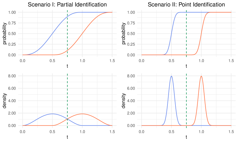
Blue lines represent the distribution of $Y(1)$ conditional on a given value of $X=x$, and red lines the distribution of $Y(0)$. Panels in the first row show the cumulative distributions and the second row the probability density. Left column shows a scenario where there is partial identification, and right column a scenario with point identification. Green dashed line represents a point $t$ where $F_{1}(t|x)-F_{0}(t|x)$ is maximized. In both scenarios $\min_{t}F_{1}(t|x)-F_{0}(t|x)=0$, for example for $t=0$.

Figure 1: Example scenarios of distributions of potential outcomes conditional on a given value of covariates $X=x$.

From equation (2.5), a sufficient condition for point identification of $\theta$ is that $\max_{t}\{F_{1}(t|x)-F_{0}(t|x)\}=1+\min_{t}\{F_{1}(t|x)-F_{0}(t|x)\}$ for all $x$. Figure 1 gives intuition for when this conditions holds, focusing on a single value of $X=x$ for ease of exposition. All panels show the conditional distributions of $Y(1)$ (in blue) and $Y(0)$ (in red), which represent the prediction of the potential outcomes given $X=x$. The upper panels show the cumulative distribution, and the lower panels the probability density. Note that predictions are not a single point since potential outcomes are random variables even conditional on $X=x$. In both scenarios $\min_{t}\{F_{1}(t|x)-F_{0}(t|x)\}=0$, for example for $t=0$, and $F_{1}(t|x)-F_{0}(t|x)$ is maximized at $t=0.75$ (green dashed line).

In the lower left panel, the distributions of $Y(1)$ and $Y(0)$ are partially overlapping, and $\max_{t}\{F_{1}(t|x)-F_{0}(t|x)\}<1+\min_{t}\{F_{1}(t|x)-F_{0}(t|x)\}=1$ (upper left panel). Since there is overlap, one cannot accurately predict if $Y(1)-Y(0)<0$ or not. For example, if an individual is at the right tail of $Y(1)$ (blue) but at the left tail of $Y(0)$ (red), then $Y(1)-Y(0)>0$. If the opposite happens, then $Y(1)-Y(0)<0$. However, since the overlap is small, the probability that $Y(1)-Y(0)<0$ is large, and the fraction harmed (for this value of $X=x$) is close to point identified. In the lower right panel the distributions are disjoint, and $\max_{t}\{F_{1}(t|x)-F_{0}(t|x)\}=1+\min_{t}\{F_{1}(t|x)-F_{0}(t|x)\}=1$ (upper right panel). In this case, even though the covariates are not informative enough to get a point-prediction of $Y(1)$ and $Y(0)$, it is informative enough to learn that $Y(1)<Y(0)$ for this value of $X=x$, and thus all individuals with $X=x$ are harmed.

Note that the interval in (2.5) is an average of $\max_{t}\{F_{1}(t|x)-F_{0}(t|x)\}$ and $1+\min_{t}\{F_{1}(t|x)-F_{0}(t|x)\}$ over all values of $X$. Hence, the figure illustrates that the informativeness of covariates in predicting the outcomes is crucial for having an narrow interval for $\theta$. In fact, if the predictions (conditional distributions) of $Y(1)$ and $Y(0)$ are disjoint for all values of $X$, then $\theta$ is point-identified. Note that in Figure 1 the green line represents the value of $s^{*}_{L}(x)$, which is the point $t$ that maximizes the distance $F_{1}(t|x)-F_{0}(t|x)$. Hence, $s^{*}_{L}(x)$ is the point that makes the two distributions as separated as possible. This fact is what motivates the notation $s$, for separator function.

3 Finite Sample Inference with Sample-Splitting

In this section, I propose sample-splitting estimators for $(\theta_{L}^{*},\theta_{U}^{*})$ and a confidence interval (CI) for $\theta$ that provides finite-sample guarantee of coverage. Given an iid sample $(Y_{i},D_{i},X_{i})_{i=1}^{n}\sim P$ that satisfies A1, the estimation strategy consists of randomly splitting the sample into two, using the first set to estimate $(s^{*}_{L},s^{*}_{U})$ with $(\hat{s}_{L},\hat{s}_{U})$, and the second set to estimate the bounds $[\max_{t}\Delta(t,\hat{s}_{L}),1+\min_{t}\Delta(t,\hat{s}_{U})]$ (as in 2.3) with a sample analogue. Conditional on the first sample, these bounds are valid due to (2.1), and finite sample inference is achieved by applying the DKW inequality (Dvoretzky et al., 1956; Massart, 1990).

I propose sample-splitting estimators for the sharp bounds $(\theta_{L}^{*},\theta_{U}^{*})$:

Definition 1 (Sample-splitting estimators).

• Randomly split the sample into two sets, denoted main and auxiliary sets. Denote by $\mathcal{I}_{M}^{1}\subset\{1,\dots,n\}$ the units in the main sample assigned to treatment, and $\mathcal{I}_{M}^{0}$ the units assigned to control;

• Using data from the auxiliary sample only, estimate $(s^{*}_{L},s^{*}_{U})$ by replacing $F_{1}(t|X)$ and $F_{0}(t|X)$ in (2.6) and (2.7) by any estimators of the conditional cdfs $\widehat{F}_{1}(t|X)$ and $\widehat{F}_{0}(t|X)$. Denote the estimators $(\hat{s}_{L},\hat{s}_{U})$.

• In the main sample, compute the final estimators

  $$\widetilde{\theta}_{L} =\max_{t}\left\{\frac{1}{|\mathcal{I}^{1}_{M}|}\sum_{i\in\mathcal{I}^{1}_{M}}\mathbb{I}\left(Y_{i}-\hat{s}_{L}(X_{i})\leq t\right)-\frac{1}{|\mathcal{I}^{0}_{M}|}\sum_{i\in\mathcal{I}^{0}_{M}}\mathbb{I}\left(Y_{i}-\hat{s}_{L}(X_{i})\leq t\right)\right\},$$

  $$\widetilde{\theta}_{U} =1+\min_{t}\left\{\frac{1}{|\mathcal{I}^{1}_{M}|}\sum_{i\in\mathcal{I}^{1}_{M}}\mathbb{I}\left(Y_{i}-\hat{s}_{U}(X_{i})\leq t\right)-\frac{1}{|\mathcal{I}^{0}_{M}|}\sum_{i\in\mathcal{I}^{0}_{M}}\mathbb{I}\left(Y_{i}-\hat{s}_{U}(X_{i})\leq t\right)\right\}.$$

$F_{1}(t|X)$ and $F_{0}(t|X)$ can be estimated with a variety of methods, including machine learning algorithms or other nonparametric estimators (see, e.g., Kneib et al., 2023 for a review). Guidelines for estimation of $\hat{s}$ are discussed in Appendix C. Although any method can be used to estimate $F_{1}(t|X)$ and $F_{0}(t|X)$, estimates $(\hat{s}_{L},\hat{s}_{U})$ closer to $(s^{*}_{L},s^{*}_{U})$ yield bounds $[\max_{t}\Delta(t,\hat{s}_{L}),1+\min_{t}\Delta(t,\hat{s}_{U})]$ that are closer to the sharp $[\max_{t}\Delta(t,s^{*}_{L}),1+\min_{t}\Delta(t,s^{*}_{U})]$, and poor estimators can lead to wider intervals.

A default choice is to make the main and auxiliary samples roughly the same size, but that is not necessary. In general, a larger auxiliary sample helps estimate $(\hat{s}_{L},\hat{s}_{U})$ closer to $(s^{*}_{L},s^{*}_{U})$, which improves the length of the target bounds $[\max_{t}\Delta(t,\hat{s}_{L}),1+\min_{t}\Delta(t,\hat{s}_{U})]$. On the other hand, a larger auxiliary sample implies a smaller main sample, which leads to larger variance of $(\widetilde{\theta}_{L},\widetilde{\theta}_{U})$ around the target bounds.

Theorem 2 (Finite-sample validity of sample-splitting CI).

Let Assumption 1 hold. Then, for any $\alpha\in(0,1)$ and any estimators $\hat{s}_{L}$ and $\hat{s}_{U}$, it holds that

$$P\left(\theta\in\left[\widetilde{\theta}_{L}-c_{\alpha},1\right]\right)\geq 1-\alpha,\;\;P\left(\theta\in\left[0,\widetilde{\theta}_{U}+c_{\alpha}\right]\right)\geq 1-\alpha,$$

$$P\left(\theta\in\left[\widetilde{\theta}_{L}-c_{\alpha/2},\widetilde{\theta}_{U}+c_{\alpha/2}\right]\right)\geq 1-\alpha.$$

where

$$c_{\alpha}=\left(\frac{\log(2/\alpha)}{2}\right)^{\frac{1}{2}}\left(\sqrt{|\mathcal{I}^{1}_{M}|}^{-1}+\sqrt{|\mathcal{I}^{0}_{M}|}^{-1}\right).$$

Theorem 2 provides confidence intervals that covers $\theta$ with probability at least $1-\alpha$ for any size of the main and auxiliary samples. Since $\theta\in[0,1]$, the one-sided CIs are particularly useful for testing $\theta=0$ or $\theta=1$. The proof of the Theorem exploits sample splitting to take $\hat{s}_{L},\hat{s}_{U}$ as given in the main sample. Then, since by (2.3) $\theta$ must lie within $[\max_{t}\Delta(t,\hat{s}_{L}),1+\min_{t}\Delta(t,\hat{s}_{U})]$, the CIs are built to cover this interval.

The finite-sample guarantee comes from the DKW inequality (Dvoretzky et al., 1956; Massart, 1990), a concentration inequality for empirical cdfs. A similar approach was implemented in Ruiz and Padilla (2022) in the context of finite-sample inference on $\theta$ in the absence of covariates. My proof differs in that I consider the splitting of the sample, and I use the one-sided version of the DKW inequality in Massart (1990) to get a smaller critical value for the one-sided CIs.

Note that a large main sample leads to $c_{\alpha}$ being close to zero, and a large auxiliary sample makes a suitable choice of $(\hat{s}_{L},\hat{s}_{U})$ closer to $(s^{*}_{L},s^{*}_{U})$. Therefore, under regularity conditions, the CIs in Theorem 2 collapse into the sharp bounds in (2.5) as both sample sizes grow to infinity. The next section investigates the large sample behavior of a similar estimator, one that allows for cross-fitting instead of sample-splitting.

4 Large Sample Inference with Cross-Fitting

The approach of the previous section uses sample splitting to provide a strong guarantee of coverage under weak conditions. In this section, I propose a new approach that uses cross-fitting, a form of sample splitting that uses the whole sample for estimating both the covariate-adjustment term and the final estimator, in order to improve power (for a discussion on cross-fitting see, for example, Chernozhukov et al., 2018).

In order to derive asymptotically valid confidence intervals, I define new regularity conditions (A2) and show in Thorem 3 an intermediate result, that the estimators are asymptotically Gaussian. The main result is then established in Theorem 4, which shows uniform validity of CIs for $\theta$. Finally, Theorem 5 shows conditions under which the CIs are exact.

Definition 2 (Cross-fitting estimators).

1. Randomly split the treatment sample into $K$ sets of same size, that is, a partition of $\{1\leq i\leq n:D_{i}=1\}$ into equal-sized folds $\{\mathcal{I}^{1}_{1},\dots,\mathcal{I}^{1}_{K}\}$. Similarly, split the control sample into $\{\mathcal{I}^{0}_{1},\dots,\mathcal{I}^{0}_{K}\}$, and denote $\mathcal{I}_{k}=\mathcal{I}^{1}_{k}\cup\mathcal{I}^{0}_{k}$;

2. For all $k\in\{1,\dots,K\}$, use data from all folds except $\mathcal{I}_{k}$ to fit estimators $\hat{s}_{L},\hat{s}_{U}$ to target $s^{*}_{L},s^{*}_{U}$, as in Definition 1.ii. Denote by $\hat{s}_{L,k},\hat{s}_{U,k}$ the estimated functions for each $k$;

3. Denote by $k(i)$ the index of the fold such that $i\in\mathcal{I}_{k(i)}$, $n_{1}=\sum_{i=1}^{n}D_{i}$ and $n_{0}=\sum_{i=1}^{n}1-D_{i}$. Compute the final estimators

   $$\widehat{\theta}_{L} =\max_{t}\Biggl{\{}\frac{1}{n_{1}}\sum_{i:D_{i}=1}\mathbb{I}(Y_{i}\leq\hat{s}_{L,k(i)}(X_{i})+t)-\frac{1}{n_{0}}\sum_{i:D_{i}=0}\mathbb{I}(Y_{i}\leq\hat{s}_{L,k(i)}(X_{i})+t)\Biggr{\}},$$

   $$\widehat{\theta}_{U} =1+\min_{t}\Biggl{\{}\frac{1}{n_{1}}\sum_{i:D_{i}=1}\mathbb{I}(Y_{i}\leq\hat{s}_{U,k(i)}(X_{i})+t)-\frac{1}{n_{0}}\sum_{i:D_{i}=0}\mathbb{I}(Y_{i}\leq\hat{s}_{U,k(i)}(X_{i})+t)\Biggr{\}}.$$

Again, several methods can be used to estimate $(\hat{s}_{L,k},\hat{s}_{U,k})$, including machine learning algorithms or other nonparametric approaches (see, e.g., Kneib et al., 2023 for a review). $K$ is assumed fixed as $n\to\infty$, and typical choices are $K=5$ or $K=10$.

In order to derive the asymptotic properties of the cross-fitting estimators, I define new regularity conditions. The results are uniform over a set of probability functions $\mathcal{P}$. This is because the literature on inference in partially identified models argues that asymptotic results have to be uniform in order to obtain approximations that accurately represent the finite-sample behavior (e.g., Imbens and Manski, 2004; Andrews and Soares, 2010). To this end, a slight revision in notation is introduced, incorporating an additional subscript $P$ for $P\in\mathcal{P}$. Consequently, $\Delta$ in (2.4) is denoted as $\Delta_{P}$, while the sharp transformations in (2.6) and (2.7) are represented by $s^{*}_{L,P}$ and $s^{*}_{U,P}$, and sharp bounds in (2.5) are $(\theta_{L,P}^{*},\theta_{U,P}^{*})$.

Assumption 2.

The set of probability functions $\mathcal{P}$ satisfies:

1. Continuity of distributions of potential outcomes: the sets of cdfs $\{t\mapsto P(Y(j)\leq t):P\in\mathcal{P}\}$ for $j=0,1$ are equicontinuous;

2. Limit of $\hat{s}_{L}$ and $\hat{s}_{U}$: There exists $s_{L,P},s_{U,P}$ for all $P\in\mathcal{P}$ such that, for all $\varepsilon>0$, $\sup_{P\in\mathcal{P}}P(|\hat{s}_{L}(X)-s_{L,P}(X)|>\varepsilon)\to 0$ and $\sup_{P\in\mathcal{P}}P(|\hat{s}_{U}(X)-s_{U,P}(X)|>\varepsilon)\to 0$ as $n\to\infty$;

3. Uniqueness of optimizers: There exists $t_{max,P},t_{min,P}$ for all $P\in\mathcal{P}$ such that, for all $\varepsilon>0$,

   $$\sup_{P\in\mathcal{P}}\sup_{t:|t-t_{max,P}|\geq\varepsilon} \Delta_{P}(t,s_{L,P})-\Delta_{P}(t_{max,P},s_{L,P})<0,$$

   $$\sup_{P\in\mathcal{P}}\sup_{t:|t-t_{min,P}|\geq\varepsilon} \Delta_{P}(t,s_{U,P})-\Delta_{P}(t_{min,P},s_{U,P})>0;$$

4. Lower bounded variance: For some $C>0$, $C<P(Y\leq s_{L,P}(X)+t_{max,P})<1-C$ and $C<P(Y\leq s_{U,P}(X)+t_{min,P})<1-C$ for all $P\in\mathcal{P}$.

Assumption 2(i) restricts the possibility of point masses in the distribution of the outcome. A2(ii) simply requires the estimators $(\hat{s}_{L},\hat{s}_{U})$ to have any limit in probability, at any rate of convergence, and allows them to be inconsistent to the sharp $(s^{*}_{L,P},s^{*}_{U,P})$. A2(iii) ensures the asymptotic distribution is first-order insensitive to the choice of the optimizers in Definition 2(iii), and it is a generalization for $P\in\mathcal{P}$ of the assumption used in Fan and Park (2010) in their approach to inference on Makarov bounds without covariates. Relaxing A2(iii) is possible and is discussed in Online Appendix III. A2(iv) is used to ensure that the problem is not trivial in the sense that $Var[\sqrt{n}\widehat{\theta}_{L}]$ and $Var[\sqrt{n}\widehat{\theta}_{U}]$ do not converge to zero. This assumption is required in order to use the result from Stoye (2009) to get asymptotic validity of the two-sided CI in Theorem 4.

Under A2(iii), the presence of the optimizers in Definition 2(iii) is asymptotically irrelevant, and $(\widehat{\theta}_{L},\widehat{\theta}_{U})$ behave as sample averages. It follows that their asymptotic distribution will be $\sqrt{n}$-Gaussian, as shown in Theorem 3. The presence of the estimated $(\hat{s}_{L,k},\hat{s}_{U,k})$ will only affect where $(\widehat{\theta}_{L},\widehat{\theta}_{U})$ are centered at, but these target bounds will always contain $\theta$, since any $s$ induces valid bounds (2.1).

Theorem 3 (Asymptotic Distribution of Cross-fitting Estimators).

Let $\mathcal{P}$ denote a set of probability functions that satisfy Assumptions 1 and 2. Then, there exists $\bar{\theta}_{L,P},\bar{\theta}_{U,P}$ with $\bar{\theta}_{L,P}\leq\theta\leq\bar{\theta}_{U,P}$ such that

$$\sqrt{n}\begin{bmatrix}\widehat{\theta}_{L}-\bar{\theta}_{L,P}\\ \widehat{\theta}_{U}-\bar{\theta}_{U,P}\end{bmatrix}\overset{d}{\to}\mathcal{N}\left(\begin{bmatrix}0\\ 0\end{bmatrix},\begin{bmatrix}\sigma^{2}_{L,P}&\sigma_{L,U,P}\\ \sigma_{L,U,P}&\sigma^{2}_{U,P}\end{bmatrix}\right)$$

uniformly in $P\in\mathcal{P}$.

Definitions of $\sigma^{2}_{L,P}$, $\sigma^{2}_{U,P}$ and $\sigma_{L,U,P}$ are provided in Appendix D. The cross-fitting estimators are asymptotically normal at the usual $\sqrt{n}$ rate, centered at bounds $[\bar{\theta}_{L,P},\bar{\theta}_{U,P}]$ that may be wider than the sharp $[\theta_{L}^{*},\theta_{U}^{*}]$, but which always contain $\theta$. The nonparametric rates of convergence of $\hat{s}_{L},\hat{s}_{U}$ only affect the target bounds $[\bar{\theta}_{L,P},\bar{\theta}_{U,P}]$, which always contain $\theta$. The resulting $\sqrt{n}$ rate is made possible through the splitting of the sample. Once conditioning on the estimated $(\hat{s}_{L,k},\hat{s}_{U,k})$ and under A2(iii), $(\widehat{\theta}_{L},\widehat{\theta}_{U})$ behave as sample averages. Conditions under which $(\bar{\theta}_{L,P},\bar{\theta}_{U,P})=(\theta_{L,P}^{*},\theta_{U,P}^{*})$ are given in Theorem 5.

Confidence intervals for $\theta$ follow from consistent sample-analogue estimators for $\sigma_{L}^{2}$, $\sigma_{U}^{2}$ and $\sigma_{L,U}$. Expressions are provided in Appendix D. One-sided confidence intervals follow directly from the normal approximation of Theorem 3. Since $\theta\in[0,1]$, the one-sided CIs are particularly useful for testing $\theta=0$ or $\theta=1$. For two-sided inference on $\theta$, I suggest using the confidence interval $\text{CI}^{3}_{\alpha}$ proposed in Stoye (2009), here denoted by $\widehat{CI}_{\alpha}$. A precise definition is reproduced in Online Appendix II.

Theorem 4 (Uniform Validity of Confidence Intervals).

Let $\mathcal{P}$ denote a set of probability functions that satisfy Assumptions 1 and 2, and denote by $\Theta(P)=[\theta_{L,P}^{*},\theta_{U,P}^{*}]$ the sharp identified set for $\theta$ when $(Y,D,X)\sim P\in\mathcal{P}$. Then,

$$\liminf_{n\to\infty}\inf_{P\in\mathcal{P}}\inf_{\theta\in\Theta(P)}P\left(\theta\geq\widehat{\theta}_{L}-z_{\alpha}\frac{\widehat{\sigma}_{L}}{\sqrt{n}}\right)\geq 1-\alpha,$$

$$\liminf_{n\to\infty}\inf_{P\in\mathcal{P}}\inf_{\theta\in\Theta(P)}P\left(\theta\leq\widehat{\theta}_{U}+z_{\alpha}\frac{\widehat{\sigma}_{U}}{\sqrt{n}}\right)\geq 1-\alpha,$$

$$\liminf_{n\to\infty}\inf_{P\in\mathcal{P}}\inf_{\theta\in\Theta(P)}P\left(\theta\in\widehat{CI}_{\alpha}\right)\geq 1-\alpha,$$

where $z_{\alpha}=\Phi^{-1}(1-\alpha)$, the $(1-\alpha)$-th quantile of the standard normal distribution.

Finally, I show that the target bounds $(\bar{\theta}_{L,P},\bar{\theta}_{U,P})$ converge to the sharp $(\theta^{*}_{L,P},\theta^{*}_{U,P})$ if the estimators of the covariate adjustment terms are consistent to the optimal at any rate. Moreover, I show that the confidence intervals are asymptotically exact under a smoothness and rate condition.

Theorem 5 (Asymptotic exactness of confidence intervals).

Let $\mathcal{P}$ denote a set of probability functions that satisfy Assumptions 1 and 2. Then, uniformly in $P\in\mathcal{P}$, $\bar{\theta}_{L,P}-\theta_{L,P}^{*}\overset{P}{\longrightarrow}0$ and $\bar{\theta}_{U,P}-\theta_{U,P}^{*}\overset{P}{\longrightarrow}0$ if respectively $s_{L,P}(x)=s^{*}_{L,P}(x)$ and $s_{U,P}(x)=s^{*}_{U,P}(x)$. Moreover, if

• The cdfs $P(Y(j)\leq t|X=x)$ for $j=0,1$ are twice continuously differentiable in $t$ with second derivative bounded uniformly in $P\in\mathcal{P}$ and $x\in\mathcal{X}$;

• Uniformly in $P\in\mathcal{P}$, $\sqrt{n}\mathbb{E}_{P}\left[\left(\hat{s}_{L,k}(X)-s^{*}_{L,P}(X)\right)^{2}|\hat{s}_{L,k}\right]\overset{P}{\longrightarrow}0$ and

  $\sqrt{n}\mathbb{E}_{P}\left[\left(\hat{s}_{U,k}(X)-s^{*}_{U,P}(X)\right)^{2}|\hat{s}_{U,k}\right]\overset{P}{\longrightarrow}0;$

then, $\sqrt{n}(\bar{\theta}_{L,P}-\theta_{L,P}^{*})\overset{P}{\longrightarrow}0$ and $\sqrt{n}(\bar{\theta}_{U,P}-\theta_{U,P}^{*})\overset{P}{\longrightarrow}0$ uniformly in $P\in\mathcal{P}$. As a consequence, under these conditions the inequalities in Theorem 4 hold with equality.

Note that a simple sufficient condition for (ii) in Theorem 5 is that $|\hat{s}_{L,k}(X)-s^{*}_{L,P}(X)|$ converges to zero at the semiparametric rate $o_{P}(n^{-1/4})$.

5 Monte Carlo Simulations

I illustrate the results of Theorems 2 and 3 with a simulation study. I also compare the performance of the sample-splitting and cross-fitting estimators, as well as the estimator proposed by Semenova (2023) and Ji et al. (2023) (denoted SJLS for the first letter of the authors’ names). Note both estimators are equivalent in the case of the DTE, and that CAIDE by construction estimates bounds that are always (weakly) narrower than SJLS (Appendix A).

For $n\in\{500,2000\}$, I simulate $10,000$ times from the following data generating process (DGP):

• $d=20$ covariates:

  • $X\sim\mathcal{N}(0,\Sigma)$, $\Sigma_{ij}=0$ if one of $i$ or $j\in\{1,2\}$, $\Sigma_{ij}=0.5^{|i-j|}$ otherwise.

• Potential outcomes:

  • $\beta_{0}=(3^{1},3^{0},0,0,\dots,0,3^{-1},3^{-2},\dots,3^{-6})$, $\Theta_{0,ij}=0.2(-1)^{i+j}$;

  • $\beta_{\tau}=(1,1,\dots,1)$, $\Theta_{\tau,ij}=0.2$;

  • $Y_{i}(0)=X^{\prime}_{i}\beta_{0}+X^{\prime}_{i}\Theta_{0}X_{i}$;

  • $Y_{i}(1)=Y_{i}(0)-1+X^{\prime}_{i}\beta_{\tau}+X^{\prime}_{i}\Theta_{\tau}X_{i}$;

  • $Y_{i}=D_{i}Y_{i}(1)+(1-D_{i})Y_{i}(0)$, $D_{i}\sim\text{Bernoulli}(0.5)$.

For this DGP, the value of $\theta$ is $\theta_{0}\approx 0.43$. I fit with $K=5$ and $\delta=0$ the models Quantile Neural Networks, Support Vector Machine (Regression) and No Covariates ($s(x)=0$). I also calculate an Oracle model that uses the sharp transformations defined in Theorem 1, which are in general unkown if the DGP is unkown. Technical details are delayed to Appendix C. I consider two scenarios: (i) $p=10$, where only covariates $X_{1}$ through $X_{10}$ are observed; (ii) $p=20$, where all $20$ covariates are observed. Note that when $p=20$, $\theta$ is point identified since potential outcomes are uniquely determined by all $20$ covariates.

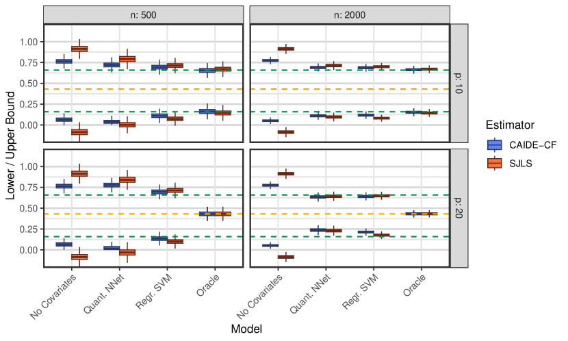
Note: Green dashed lines represent the sharp identified set of $\theta$ when $p=10$, and orange dashed lines represent the true value of $\theta$. Boxplots are composed by the median, two hinges at the first and third quartiles, and whiskers extending to the most extreme data points no further than 1.5 times the interquartile range (third minus first quartile) from the hinge.

Figure 2: Distribution of Estimators for Lower and Upper Bounds on $\theta$

Figure 2 shows the distribution of the estimators CAIDE-CF (Cross Fitting) and SJLS for the lower and upper bounds on $\theta$, for $n=500,2000$ and scenarios $p=10,20$. It illustrates the fact that the estimators are centered around bounds determined by the different models for estimating $\hat{s}$. Some models perform better than others in yielding narrower bounds. In most cases, for example, the Regr. SVM model led to the narrowest bounds, close to the sharp bounds in the $p=10$ case. A larger sample size leads to smaller variation in the estimators. Observing all $p=20$ covariates, instead of $p=10$, can lead to narrower bounds (e.g., Regr. SVM and $n=2000$) but also to wider bounds if the sample is smaller (Quant. NNet and $n=500$). Throughout, the estimates of CAIDE are narrower than SJLS.

In Table 1, I show the probability of rejecting the hypotheses $H_{0}:\theta=0$ and $H_{0}:\theta\geq\theta_{0}$, using the one-sided confidence interval based on the lower bound in Theorem 4. Here, $\theta_{0}\approx 0.43$ is the true value of $\theta$ for this DGP. A high rejection rate for the first hypothesis indicates power, since $0$ is not in the sharp identified set of $\theta$. The rejection rate of the second hypothesis indicates size and ideally should be smaller than or equal to the nominal $0.05$. I also measure the average length of the confidence intervals, defined as the distance between the lower and upper bounds calculated from the one-sided CIs in Theorem 4. I compare $n=500,2000$ and $p=10,20$, for different models and estimators. CAIDE-SS is the sample-splitting estimator of Section 3, and CAIDE-CF is the cross-fitting estimator of Section 4. The table shows that including covariates, having a larger sample size, or observing all $20$ covariates all increase power while preserving size. The sample-splitting estimators are conservative, and exhibit the largest average length for Regr. SVM. Still, it often demonstrates some power, for example it excludes zero in $99.4\%$ of the cases when $p=20$, $n=2000$ and the model is Regr. SVM. The cross-fitting estimator performs better than SJLS in terms of smaller confidence intervals while preserving coverage, and it achieves the nominal coverage rate for the oracle model when $p=20$.

Table 1: Measures of power and coverage for lower bound on $\theta$

		p = 10			p = 20
n	Estimator	$\theta=0$	$\theta\geq\theta_{0}$	Avg Length	$\theta=0$	$\theta\geq\theta_{0}$	Avg Length
No Covariates
$500$	Sample Split.	$0.000$	$0.000$	$0.998$	$0.000$	$0.000$	$0.998$
$500$	Cross Fit.	$0.722$	$0.000$	$0.802$	$0.722$	$0.000$	$0.802$
$500$	SJLS	$0.000$	$0.000$	$1.000$	$0.000$	$0.000$	$1.000$
$2,000$	Sample Split.	$0.001$	$0.000$	$0.892$	$0.001$	$0.000$	$0.892$
$2,000$	Cross Fit.	$0.983$	$0.000$	$0.776$	$0.983$	$0.000$	$0.776$
$2,000$	SJLS	$0.000$	$0.000$	$0.965$	$0.000$	$0.000$	$0.965$
Regr. SVM
$500$	Sample Split.	$0.004$	$0.000$	$0.935$	$0.007$	$0.000$	$0.948$
$500$	Cross Fit.	$0.970$	$0.000$	$0.698$	$0.998$	$0.000$	$0.676$
$500$	SJLS	$0.806$	$0.000$	$0.815$	$0.964$	$0.000$	$0.791$
$2,000$	Sample Split.	$0.414$	$0.000$	$0.804$	$0.994$	$0.000$	$0.716$
$2,000$	Cross Fit.	$1.000$	$0.000$	$0.628$	$1.000$	$0.000$	$0.485$
$2,000$	SJLS	$1.000$	$0.000$	$0.707$	$1.000$	$0.000$	$0.562$
Oracle
$500$	Cross Fit.	$0.999$	$0.000$	$0.608$	$1.000$	$0.051$	$0.103$
$2,000$	Cross Fit.	$1.000$	$0.000$	$0.568$	$1.000$	$0.049$	$0.052$

6 Application to Microcredit

In 2022, microcredit reached more than 170 million borrowers worldwide, with a total loan portfolio of over $140 billion (Convergences, 2023). Theory suggests that microborrowing can be beneficial or harmful (Banerjee, 2013, Garz et al., 2021), and evidence suggests that average effects are small if not negligible (Banerjee et al., 2015b, Meager, 2019). Analysis of heterogeneity mostly relied on rank preservation, and suggested mainly positive impact in the upper tail of income/profits distributions (e.g., Meager, 2022). Yet, evidence of negative effects has been scarce. I revisit five studies which randomized offering a microloan at the individual level, and find evidence of both positive and negative treatment effects of microcredit. A brief description of the datasets is presented in Table 2.

CAIDE is able to provide informative bounds, even in this challenging context. First because the distributions of income/profits are similar between treated and control groups. This is reflected in not statistically significant ATEs in Table 2, and estimated $[\theta_{L},\theta_{U}]$ close to $[0,1]$ if covariates are not considered (Table 3). Second, because the sample sizes are relatively small (ranging from 548 to 1964), with a large number of covariates (from 24 to 97). Finally, because predicting business outcomes is itself a difficult task (McKenzie and Sansone, 2019).

Table 2: Description of datasets in microcredit

Country	Bosnia	Egypt	Philippines (1)	Phil. (2)	S. Africa
Year of implementation	2009	2016	2006	2010	2004
Treated/control obs.	551/444	477/478	891/222	1651/313	235/313
Number of covariates	48	97	24	39	33
Avg. loan size in treatment group (USD PPP)	$1,389	$9,912	$1,045	$492	$180
Avg household income at endline (USD PPP)	$21,735	$26,844	$12,173	$10,280	$14,845
ATE in Household Income (t-statistic)	$609 (0.593)	$1,224 (0.573)	$1,374 (0.819)	$110 (0.103)	-$520 (-0.159)

• Study citations respectively: Augsburg et al. (2015), Bryan et al. (2021), Karlan and Zinman (2011), Karlan et al. (2016), Karlan and Zinman (2010).

Using $K=10$, I fit the estimators of Section 4. For each fold, I fit another layer of sample splitting to pick via $10-$fold cross-validation one of the models: Quantile Forests, Quantile Neural Networks, Random Forest (Regression), Neural Networks (Reg.), Elastic Net (Reg.), Extreme Gradient Boosting (Reg.), and Constant ($s(X)=0)$. Technical details are provided in Appendix C.

Table 3: Bounds on fraction harmed by microcredit - household income

	Lower Bound			Upper Bound
	CAIDE	No Covariates	SJLS	CAIDE	No Covariates	SJLS
Bosnia	0.108 (0.030) [0.000]	0.040 (0.027) [0.073]	0.024 (0.036) [0.254]	0.946 (0.028) [0.028]	0.973 (0.031) [0.195]	0.977 (0.047) [0.310]
Egypt	0.260 (0.022) [0.000]	0.009 (0.014) [0.263]	0.248 (0.033) [0.000]	0.787 (0.022) [0.000]	0.966 (0.021) [0.051]	0.792 (0.033) [0.000]
Philippines (1)	0.083 (0.039) [0.018]	0.071 (0.039) [0.036]	0.077 (0.053) [0.075]	0.971 (0.019) [0.057]	0.931 (0.027) [0.005]	1.048 (0.049) [1.000]
Philippines (2)	0.145 (0.033) [0.000]	0.022 (0.018) [0.103]	0.075 (0.034) [0.013]	0.739 (0.032) [0.000]	0.951 (0.032) [0.062]	0.751 (0.047) [0.000]
South Africa	0.028 (0.017) [0.053]	0.033 (0.018) [0.036]	-0.017 (0.054) [1.000]	0.876 (0.043) [0.002]	0.913 (0.043) [0.021]	0.938 (0.049) [0.105]
All	0.125 (0.013) [0.000]	0.035 (0.008) [0.000]	0.081 (0.019) [0.000]	0.864 (0.013) [0.000]	0.947 (0.010) [0.000]	0.901 (0.020) [0.000]

• Standard errors in parentheses, and p-values in brackets. The null hypothesis for the lower bound is $\theta^{*}_{L}=0$, and for the upper bound $\theta^{*}_{U}=1$. Response variable: $log(1+household\ income)$.

Table 3 shows the estimates for the lower and upper bounds on $\theta$ for $\delta=0$ using CAIDE with and without covariates. The outcome is the logarithm of annual household income. Considering that the outcome is continuous, it follows that $\theta=P(Y(1)-Y(0)\leq 0)=P(Y(1)-Y(0)<0)$, the lower bound on $\theta$ is the minimum proportion of households that have a negative effect from the microloan, and the upper bound is the maximum proportion. Note that one minus the upper bound denotes the minimum proportion of households that have a positive effect. Results for $\delta=-0.05$ and $\delta=0.05$ are similar and are presented in Table 4. In Bosnia, for example, I estimate that at least $10.8\%$ of the households would be better off without the microloan (p-value $<10^{-3}$), and at most $94.6\%$ have negative effects (p-value $0.028$). That is, at least $6.4\%$ are better off ($1-0.946$). Overall, I find significant lower bounds at the $10\%$ level for all of the five datasets, and at the $5\%$ level for four of them. As for the upper bound, I find statistical significance at $5\%$ in four of the datasets. These results reveal important presence of heterogeneity, even when the ATEs are not statistically significant (Table 2).

Incorporating covariates makes substantial difference in many of the point estimates. In Egypt, for example, the lower bound without covariates is $0.009$ (p-value $0.264$), whereas incoporating covariates improves the estimate to $0.260$ (p-value $<10^{-3}$). The differences between the point estimates with and without covariates are siginificant at the $5\%$ level for both lower and upper bounds for Egypt, Philippines (2) and All.

Table 3 also illustrates how CAIDE can outperform SJLS (Semenova, 2023, Ji et al., 2023) in terms of narrower confidence intervals. In the case of the lower bound for Bosnia, for example, it is estimated $10.8\%$ with CAIDE vs $2.4\%$ with SJLS, leading to substancial difference in p-values ($<10^{-3}$ vs $0.254$). It also illustrates how SJLS can estimate negative lower bounds (South Africa), or upper bounds that are greater than one (Philippines (1)). In both cases, the estimates with CAIDE are statistically significant at the $10\%$ level.

Table 5 in Online Appendix IV shows results for business profits. Again, including covariates improves the bounds. Averaging estimates from all datasets, I find that at least $10.8\%$ (p-value $<10^{-3}$) of the population was harmed, and at least $9.8\%$ (p-value $<10^{-3}$) benefited from microcredit.

An important note is that this evidence does not inform the nature of the negative effects or their magnitude. It could be the case, for example, that the negative outcomes are relatively small and are a natural consequence of investments being risky. In that case, the decision to take a microloan could still be rational if the prospect of gains is better than the risk of loss.

7 Conclusion

I propose two novel inference approaches to the distributional treatment effect $\theta=P(Y(1)-Y(0)\leq\delta)$, for any fixed $\delta$. A new characterization of the sharp identified set of $\theta$ is provided, which is based on covariate adjustment. It has the desirable property of being robust to the choice of the covariate-adjustment term $s(x)$, in the sense that if this term is misspecified, the identified set is wider but still valid. As a consequence, any method can be used to estimate $s$, including machine learning algorithms. I provide finite-sample valid inference using sample-splitting and asymptotic inference using cross-fitting, which is also asymptotically exact under additional conditions.

The practical relevance of the method is illustrated in a simulation study and in an application to microcredit. The application reveals important presence of heterogeneity, with significant negative and positive treatment effects. The results show that the method is able to provide informative bounds even in challenging contexts, such as when the ATE is not statistically significant, the sample size is small, and the number of covariates is large.

By using CAIDE, an applied researcher can learn more about heterogeneous effects not only by gathering larger samples, but also by collecting information on covariates that help predict potential outcomes.

Appendix A Comparison with Semenova (2023) and Ji et al. (2023)

I compare the asymptotic properties of CAIDE with the estimators proposed by Semenova (2023) and Ji et al. (2023) (denoted by SJLS for the first letter of the names of the authors). I focus on the cross-fitting version of the estimators (Definition 2(iii)), and compare them to the cross-fitting estimators in SJLS. Note that in the case of the DTE $\theta$, the estimators of Semenova (2023) and Ji et al. (2023) are equivalent.

Since SJLS consider a known propensity score, I compare SJLS to a version of CAIDE that uses the true propensity score (Online Appendix I) instead of using the fraction of treated units in the sample. In Appendix B I show that using the actual number of treated units (as in Definition 2(iii)) instead of the known propensity score leads to the same asymptotic distribution but with a smaller asymptotic variance. Hence, using the true propensity score in CAIDE is the natural comparison. I focus on the lower bound for simplicity, and analogous results hold for the upper bound. Define

$$\widehat{\Delta}(t)=\frac{1}{n}\sum_{i=1}^{n}\biggl{(}\frac{D_{i}}{p(X_{i})}\mathbb{I}(Y_{i}\leq\hat{s}_{L,k(i)}(X_{i})+t)-\frac{1-D_{i}}{1-p(X_{i})}\mathbb{I}(Y_{i}\leq\hat{s}_{L,k(i)}(X_{i})+t)\biggr{)}$$

Then, CAIDE is equivalent to $\hat{\theta}_{C}:=\max_{t}\widehat{\Delta}(t)$ and SJLS is given by $\hat{\theta}_{S}:=\widehat{\Delta}(0)$. Theorem 3 of this paper is comparable to Theorem 4.1 in Semenova (2023), and Theorem 3.1 and Proposition 3.2 in Ji et al. (2023). They all show asymptotic validity of confidence intervals. Define confidence intervals as $CI_{C}$ for CAIDE and $CI_{S}$ for SJLS. Since by construction $\hat{\theta}_{C}\geq\hat{\theta}_{S}$, it follows that $\hat{\theta}_{C}$ first order stochastically dominates $\hat{\theta}_{S}$. Under the conditions of these theorem, it follows that, for any sequence $\theta_{n}<\theta_{P_{n}}^{*}$, where $\theta_{P_{n}}^{*}$ is the sharp lower bound as in (2.5),

$$\liminf_{n\to\infty}P_{n}(\theta_{n}\in CI_{S})-P(\theta_{n}\in CI_{C})\geq 0.$$

Hence, $CI_{C}$ has more power than $CI_{S}$ in the sense that $CI_{S}$ may include elements below the sharp lower bound that are not included in $CI_{C}$. Note that validity of $CI_{C}$ relies on A2(iii), on the uniqueness of the maximizer of $\widehat{\Delta}(t)$, which is not assumed in SJLS.

Appendix B Estimated vs True Propensity Score

I show that, when the propensity score is constant, the asymptotic variances of the estimators in 2(iii) are smaller than those of alternative estimators that consider the true propensity score. When the propensity score is known and not constant as in A1.ii, an alternative estimator that uses the true propensity score is proposed in Online Appendix I-B. The lower bound, for example, is given by

$$\widehat{\theta}^{B}_{L} =\max_{t}\Biggl{\{}\frac{1}{n}\sum_{i=1}^{n}\biggl{(}\frac{D_{i}}{p(X_{i})}\mathbb{I}(Y_{i}\leq\hat{s}_{L,k(i)}(X_{i})+t)$$

$$\hskip 60.0pt-\frac{1-D_{i}}{1-p(X_{i})}\mathbb{I}(Y_{i}\leq\hat{s}_{L,k(i)}(X_{i})+t)\biggr{)}\Biggr{\}}.$$

Now, note that the estimators in Definition 2(iii) can be rewritten in terms of an estimated propensity score $\hat{p}=\frac{1}{n}\sum_{i=1}^{n}D_{i}$. For the lower bound, we have

$$\widehat{\theta}_{L} \equiv\max_{t}\Biggl{\{}\frac{1}{n}\sum_{i=1}^{n}\biggl{(}\frac{D_{i}}{\hat{p}}\mathbb{I}(Y_{i}\leq\hat{s}_{L,k(i)}(X_{i})+t)$$

$$\hskip 60.0pt-\frac{1-D_{i}}{1-\hat{p}}\mathbb{I}(Y_{i}\leq\hat{s}_{L,k(i)}(X_{i})+t)\biggr{)}\Biggr{\}}.$$

Now, let $t_{L,P}=t_{max,P}$; $t_{U,P}=t_{min,P}$; $\pi=P(D=1)$ (as in A1). For $A\in\{L,U\}$ and $j\in\{0,1\}$, define $Z_{A,P}(j)=\mathbb{I}(Y(j)\leq s_{A,P}(X)+t_{A,P})$. Then, the asymptotic variance of $\widehat{\theta}_{A}$ (as in Definition 2(iii)) is given by:

$$\frac{Var[Z_{A,P}(1)]}{\pi}+\frac{Var[Z_{A,P}(0)]}{1-\pi}$$

Now, if $p(x)=\pi$, the asymptotic variance of $\widehat{\theta}^{B}_{A}$ simplifies to:

$$\frac{Var[Z_{A,P}(1)]}{\pi}+\frac{Var[Z_{A,P}(0)]}{1-\pi}+\left(\frac{\mathbb{E}[Z_{A,P}(1)]}{\pi}-\frac{\mathbb{E}[Z_{A,P}(0)]}{1-\pi}\right)^{2}\pi(1-\pi)$$

Since the third term above is never negative and in general different from zero, the asymptotic variance of $\widehat{\theta}_{A}$ is smaller than the one of $\widehat{\theta}^{B}_{A}$.

The result that using the estimated propensity score yields smaller asymptotic variance than using the true propensity score is similar to other results in the literature (e.g., Hirano et al., 2003 in the context of the ATE).

Appendix C Estimation of the covariate-adjustment term

I consider two approaches to estimate the covariate-adjustment term $s(x)$. I focus the explanation on the case of the lower bound for simplicity. First, I estimate $\hat{F}_{j}(t|x)$ ($j=0,1$) with one of two methods, and then I calculate $\hat{s}$ from $\hat{F}_{j}(t|x)$.

The first method for estimating $\hat{F}_{j}(t|x)$ is to use quantile models, such as quantile forests or quantile neural networks. They give estimates for quantiles, that is, $\hat{F}^{-1}_{j}(\tau|x)$, for all values of $x$ in the sample. $\hat{F}_{j}(t|x)$ can be calculated from $\hat{F}^{-1}_{j}(\tau|x)$ by linear interpolation. In Sections 5 and 6, I consider a grid for $\tau$ from $0$ to $1$ by increments of $0.01$, i.e. $\tau_{k}\in\{0,0.01,\dots,1\}$. For an arbitrary $t$, pick $\tau_{a}$ and $\tau_{b}$ such that $t_{a}=\hat{F}^{-1}_{j}(\tau_{a}|x),t_{b}=\hat{F}^{-1}_{j}(\tau_{b}|x)$ are the two closest values to $t$ such that $t_{a}\leq t\leq t_{b}$. Then, $\hat{F}_{j}(t|x)=\tau_{a}+\frac{\tau_{b}-\tau_{a}}{t_{b}-t_{a}}(t-t_{a})$.

The second method for estimating $\hat{F}_{j}(t|x)$ assumes that the distribution of $Y(j)|X=x$ is the same for all $x$ up to a shift in the mean $\mathbb{E}[Y(j)|X=x]$. This is allowed by the framework of Theorems 2 and 3 since misspecification of $s^{*}$ leads to valid even if wider bounds. Denote by $\hat{\mu}(x)$ an estimator of $\mathbb{E}[Y(j)|X=x]$, using any regression method. For example, in Section 5 I use Support Vector Machine. Denote by $\hat{F}_{e}(t)$ the empirical cdf of the residuals $Y(j)-\hat{\mu}(X)$ inside the training sample. Then, $\hat{F}_{j}(t|x)=\hat{F}_{e}(t-\hat{\mu}(x))$.

Once $\hat{F}_{j}(t|x)$ is estimated, the covariate-adjustment term is calculated by $\hat{s}(x)=\arg\max_{t\in\mathcal{T}}\left\{\hat{F}_{1}(t|x)-\hat{F}_{0}(t|x)\right\}$. For $\mathcal{T}$, I use a random grid of size $10^{4}$ from a normal distribution of mean $0$ and standard deviation $\max(Y)-\min(Y)$.

I fit all models in R. For quantile neural networks, I use the package qrnn with 3 hidden nodes, in 1 trial and maximum of 100 iterations. Other parameters are the default choice. For quantile random forests, I use the package ranger with 1,000 trees and otherwise default hyperparameters. For all the regression methods, I use the package mlr3 with default values of hyperparameters. The packages for all models, used through mlr3 are: random forests (ranger), extreme gradient boosting (xgboost), support vector machine (e1071), neural networks (nnet), elastic net (glmnet). The constant/none model simply takes $s(x)=0$.

For choosing the best model in the application of Section 6, I use cross validation inside each fold. That is, for each fold, I fit all the models in a 10-fold cross-validation, and choose the model that gives the largest (smallest) lower (upper) bound. Note that the test set is never used in this approach.

When calculating the sample-splitting estimators and confidence intervals of Section 3, I use a 50-50 split of the sample.

Appendix D Definitions Ommited from the Main Text

Let $t_{L,P}=t_{max,P}$; $t_{U,P}=t_{min,P}$; $\pi=P(D=1)$ (as in A1); For $A\in\{L,U\}$ and $j\in\{0,1\}$, define $Z_{A,P}(j)=\mathbb{I}(Y(j)\leq s_{A,P}(X)+t_{A,P})$; $\sigma^{2}_{A,P}(j)=Var[Z_{A,P}(j)]$. Then, for $A\in\{L,U\}$:

$$\sigma^{2}_{A,P}=\frac{Var[Z_{A,P}(1)]}{\pi}+\frac{Var[Z_{A,P}(0)]}{1-\pi}$$

and

$$\sigma_{L,U,P}=\frac{Cov[Z_{L,P}(1),Z_{U,P}(1)]}{\pi}+\frac{Cov[Z_{L,P}(0),Z_{U,P}(0)]}{1-\pi}$$

For the sample analogues, for $A\in\{L,U\}$ define

$$\widehat{F}_{A,j}(t)=\frac{1}{n_{j}}\sum_{i:D_{i}=j}\mathbb{I}(Y_{i}\leq\hat{s}_{A,k(i)}(X_{i})+t);$$

$$\hat{t}_{L}=\arg\max_{t}\widehat{F}_{A,1}(t)-\widehat{F}_{A,0}(t);\ \hat{t}_{U}=\arg\min_{t}\widehat{F}_{A,1}(t)-\widehat{F}_{A,0}(t);$$

$$\hat{\sigma}^{2}_{A,j}=\frac{1}{n_{j}}\sum_{i:D_{i}=j}\left[\mathbb{I}(Y_{i}\leq\hat{s}_{A,k(i)}(X_{i})+\hat{t}_{A})-\widehat{F}_{A,j}(\hat{t}_{A})\right]^{2};$$

$$\hat{\sigma}_{L,U,j}=$$

$$\frac{1}{n_{j}}\sum_{i:D_{i}=j}\left[\mathbb{I}(Y_{i}\leq\hat{s}_{L,k(i)}(X_{i})+\hat{t}_{L})-\widehat{F}_{L,j}(\hat{t}_{L})\right]\left[\mathbb{I}(Y_{i}\leq\hat{s}_{U,k(i)}(X_{i})+\hat{t}_{U})-\widehat{F}_{U,j}(\hat{t}_{U})\right];$$

and $\hat{\pi}=n_{1}/n$. Then, for $A\in\{L,U\}$,

$$\hat{\sigma}^{2}_{A}=\frac{\hat{\sigma}^{2}_{A,1}}{\hat{\pi}}+\frac{\hat{\sigma}^{2}_{A,0}}{1-\hat{\pi}};\quad\hat{\sigma}_{L,U}=\frac{\hat{\sigma}_{L,U,1}}{\hat{\pi}}+\frac{\hat{\sigma}_{L,U,0}}{1-\hat{\pi}}.$$

Appendix E Proofs of the Main Results

Proof of Theorem 2.

For the case of the lower bound, denote for $j=0,1$

$$\hat{F}_{j,L}(t)=\frac{1}{|\mathcal{I}^{j}_{M}|}\sum_{i\in\mathcal{I}^{j}_{M}}\mathbb{I}\left(Y_{i}-\hat{s}_{L}(X_{i})\leq t\right)$$

Let $\mathcal{I}_{A}$ denote the auxiliary sample, and let $F_{j,L}(t)=\mathbb{E}[\hat{F}_{j,L}(t)|\mathcal{I}_{A}]$ for $j=0,1$ denote the true cdf of $Y(j)-\hat{s}_{L}(X)$ taking $\hat{s}_{L}$ as fixed. Let $\hat{t}_{max}\in\arg\max_{t}[\hat{F}_{1,L}(t)-\hat{F}_{0,L}(t)]$.

Then, we have that $\widetilde{\theta}_{L}=\hat{F}_{1,L}(\hat{t}_{max})-\hat{F}_{0,L}(\hat{t}_{max})$. Finally, denote $c_{\alpha,1}=\left(\frac{\log(2/\alpha)}{2|\mathcal{I}^{M}_{1}|}\right)^{1/2}$, $c_{\alpha,0}=\left(\frac{\log(2/\alpha)}{2|\mathcal{I}^{M}_{0}|}\right)^{1/2}$.

I first focus on the case of the one-sided interval $P\left(\theta\in\left[\widetilde{\theta}_{L}-c_{\alpha},1\right]\right)$. Note that $F_{1,L}(t)-F_{0,L}(t)$ is a valid lower bound by (2.3) for any $t$ and $\hat{s}_{L}$. Thus, $\theta\in[F_{1,L}(\hat{t}_{max})-F_{0,L}(\hat{t}_{max}),1]$ and $F_{1,L}(\hat{t}_{max})-F_{0,L}(\hat{t}_{max})\leq\theta$. Then,

$$P\left(\theta\in\left[\widetilde{\theta}_{L}-c_{\alpha},1\right]\right)$$

$$\geq P\left(F_{1,L}(\hat{t}_{max})-F_{0,L}(\hat{t}_{max})\geq\widetilde{\theta}_{L}-c_{\alpha}\right)$$

$$=1-P\left(\left[\hat{F}_{1,L}(\hat{t}_{max})-F_{1,L}(\hat{t}_{max})\right]+\left[F_{0,L}(\hat{t}_{max})-\hat{F}_{0,L}(\hat{t}_{max})\right]>c_{\alpha}\right)$$

$$\geq 1-P\left(\left[\hat{F}_{1,L}(\hat{t}_{max})-F_{1,L}(\hat{t}_{max})\right]>c_{\alpha,1}\lor\left[F_{0,L}(\hat{t}_{max})-\hat{F}_{0,L}(\hat{t}_{max})\right]>c_{\alpha,0}\right)$$

$$\geq 1-P\left(\hat{F}_{1,L}(\hat{t}_{max})-F_{1,L}(\hat{t}_{max})>c_{\alpha,1}\right)-P\left(F_{0,L}(\hat{t}_{max})-\hat{F}_{0,L}(\hat{t}_{max})>c_{\alpha,0}\right)$$

$$=1-P\left(\hat{F}_{1,L}(\hat{t}_{max})-F_{1,L}(\hat{t}_{max})>c_{\alpha,1}\right)$$

$$\hskip 20.0pt-P\left(\hat{F}_{0,L}(\hat{t}_{max})-F_{0,L}(\hat{t}_{max})>c_{\alpha,0}\right)$$ (E.1)

$$\geq 1-P\left(\sup_{t}\left(\hat{F}_{1,L}(t)-F_{1,L}(t)\right)>c_{\alpha,1}\right)-P\left(\sup_{t}\left(\hat{F}_{0,L}(t)-F_{0,L}(t)\right)>c_{\alpha,0}\right)$$

$$=1-\mathbb{E}\left[P\left(\sup_{t}\left(\hat{F}_{1,L}(t)-F_{1,L}(t)\right)>c_{\alpha,1}\Bigm{|}\mathcal{I}_{A}\right)\right]$$

$$\hskip 15.0pt-\mathbb{E}\left[P\left(\sup_{t}\left(\hat{F}_{0,L}(t)-F_{0,L}(t)\right)>c_{\alpha,0}\Bigm{|}\mathcal{I}_{A}\right)\right]$$ (E.2)

$$\geq 1-\mathbb{E}\left[\exp{(-2|\mathcal{I}^{M}_{1}|c_{\alpha,1}^{2})}\right]-\mathbb{E}\left[\exp{(-2|\mathcal{I}^{M}_{0}|c_{\alpha,0}^{2})}\right]$$ (E.3)

$$=1-\exp{(-2|\mathcal{I}^{M}_{1}|c_{\alpha,1}^{2})}-\exp{(-2|\mathcal{I}^{M}_{0}|c_{\alpha,0}^{2})}$$

$$=1-\alpha$$

(E.1) holds since $\hat{F}_{0,L}(t)-F_{0,L}(t)$ is symmetric around zero for all $t$. (E.2) holds by the law of iterated expectations, and note the expected values are in respect to $\mathcal{I}_{A}$. (E.3) holds by the one-sided DKW inequality as in Massart (1990). Note the use of sample splitting and conditioning on the auxiliary set $\mathcal{I}_{A}$ is important since it ensures that $(Y_{i},\hat{s}_{L}(X_{i}),D_{i})_{i\in\mathcal{I}^{1}_{M}\cup\mathcal{I}^{0}_{M}}$ are iid, assumption required for the DKW inequality.

The proof for $P\left(\theta\in\left[0,\widetilde{\theta}_{U}+c_{\alpha}\right]\right)\geq 1-\alpha$ is analogous. Finally, the validity of the two-sided confidence interval follows immediately:

$$P\Biggl{(}\theta\in\left[\widetilde{\theta}_{L}-c_{\alpha/2},\widetilde{\theta}_{U}+c_{\alpha/2}\right]\Biggr{)} =P\Biggl{(}\theta\in\left[\widetilde{\theta}_{L}-c_{\alpha/2},1\right]\land\theta\in\left[0,\widetilde{\theta}_{U}+c_{\alpha/2}\right]\Biggr{)}$$

$$=1-P\Biggl{(}\theta\not\in\left[\widetilde{\theta}_{L}-c_{\alpha/2},1\right]\lor\theta\not\in\left[0,\widetilde{\theta}_{U}+c_{\alpha/2}\right]\Biggr{)}$$

$$\geq 1-P\Biggl{(}\theta\not\in\left[\widetilde{\theta}_{L}-c_{\alpha/2},1\right]\Biggr{)}-P\Biggl{(}\theta\not\in\left[0,\widetilde{\theta}_{U}+c_{\alpha/2}\right]\Biggr{)}$$

$$\geq 1-\alpha/2-\alpha/2$$

$$=1-\alpha$$

∎

Definitions used in the proofs of the results of Section 4:

• $t_{L,P}=t_{max,P},\ t_{U,P}=t_{min,P}$;

• $F_{P,j}(t,s)=P(Y(j)\leq s(X)+t)$ (note $F_{P,j}(t,s)$ is random if $t$ and/or $s$ are random);

• $\mathcal{I}_{j,k}=\{i\in\{1,\dots,n\}:D_{i}=j\land i\in\mathcal{I}_{k}\}$;

• $\widehat{F}_{j,k}(t,s)=\frac{1}{n_{j}/K}\sum_{i\in\mathcal{I}_{j,k}}\mathbb{I}(Y_{i}\leq s(X_{i})+t)$;

• $\hat{t}_{L}=\arg\max_{t}\frac{1}{K}\sum_{k=1}^{K}\left[\widehat{F}_{1,k}(t,\hat{s}_{L,k})-\widehat{F}_{0,k}(t,\hat{s}_{L,k})\right]$;

• $\hat{t}_{U}=\arg\min_{t}\frac{1}{K}\sum_{k=1}^{K}\left[\widehat{F}_{1,k}(t,\hat{s}_{U,k})-\widehat{F}_{0,k}(t,\hat{s}_{U,k})\right]$;

• $\hat{\pi}=n_{1}/n$.

Theorem 3 is restated as Theorem E.1:

Theorem E.1 (Asymptotic distribution of cross-fitting estimators).

Let $\mathcal{P}$ denote a set of probability functions that satisfy Assumptions 1 and 2. Let $\{P_{n}\}_{n\geq 1}\subset\mathcal{P}$ be a sequence of probability functions such that

$$\begin{pmatrix}\sigma^{2}_{L,P_{n}}&\sigma_{L,U,P_{n}}\\ \sigma_{L,U,P_{n}}&\sigma^{2}_{U,P_{n}}\end{pmatrix}\to\begin{pmatrix}\sigma^{2}_{L}&\sigma_{L,U}\\ \sigma_{L,U}&\sigma^{2}_{U}\end{pmatrix}$$

for some $\sigma^{2}_{L},\sigma^{2}_{U}\geq 0$ and $\sigma_{L,U}\in\mathbb{R}$.

Then, there exists $\bar{\theta}_{L,P_{n}},\bar{\theta}_{U,P_{n}}$ with $\bar{\theta}_{L,P_{n}}\leq\theta_{L,P_{n}}^{*}\leq\theta_{P_{n}}\leq\theta_{U,P_{n}}^{*}\leq\bar{\theta}_{U,P_{n}}$ such that

$$\sqrt{n}\begin{bmatrix}\widehat{\theta}_{L}-\bar{\theta}_{L,P_{n}}\\ \widehat{\theta}_{U}-\bar{\theta}_{U,P_{n}}\end{bmatrix}\overset{d}{\to}\mathcal{N}\left(\begin{bmatrix}0\\ 0\end{bmatrix},\begin{bmatrix}\sigma^{2}_{L}&\sigma_{L,U}\\ \sigma_{L,U}&\sigma^{2}_{U}\end{bmatrix}\right)$$

Proof of Theorem E.1.

For $A\in\{L,U\}$, define

• $\bar{\theta}_{A,P,k}=F_{P,1}(\hat{t}_{A},\hat{s}_{A,k})-F_{P,0}(\hat{t}_{A},\hat{s}_{A,k})$,

• $\bar{\theta}_{A,P}=\frac{1}{K}\sum_{k=1}^{K}\bar{\theta}_{A,P,k}$,

• $\widehat{\theta}_{A,k}=\widehat{F}_{1,k}(\hat{t}_{A},\hat{s}_{A,k})-\widehat{F}_{0,k}(\hat{t}_{A},\hat{s}_{A,k})$.

Note that $\widehat{\theta}_{A}=\frac{1}{K}\sum_{k=1}^{K}\widehat{\theta}_{A,k}$, and that

$$\widehat{\theta}_{A,k}-\bar{\theta}_{A,P_{n},k}=\left[\widehat{F}_{1,k}(\hat{t}_{A},\hat{s}_{A,k})-F_{P_{n},1}(\hat{t}_{A},\hat{s}_{A,k})\right]-\left[\widehat{F}_{0,k}(\hat{t}_{A},\hat{s}_{A,k})-F_{P_{n},0}(\hat{t}_{A},\hat{s}_{A,k})\right]$$

The proof consists in showing, for $A\in\{L,U\}$ and $j=0,1$, that

$$\sqrt{\frac{n_{j}}{K}}\left(\widehat{F}_{j,k}(\hat{t}_{A},\hat{s}_{A,k})-F_{P_{n},j}(\hat{t}_{A},\hat{s}_{A,k})\right)$$

$$=\sqrt{\frac{n_{j}}{K}}\left(\widehat{F}_{j,k}(\hat{t}_{A},s_{A,P_{n}})-F_{P_{n},j}(\hat{t}_{A},s_{A,P_{n}})\right)+o_{P_{n}}(1)$$ (E.4)

$$=\sqrt{\frac{n_{j}}{K}}\left(\widehat{F}_{j,k}(t_{A,P_{n}},s_{A,P_{n}})-F_{P_{n},j}(t_{A,P_{n}},s_{A,P_{n}})\right)+o_{P_{n}}(1)$$ (E.5)

Finally, I show

$$\sqrt{n}\begin{bmatrix}\widehat{\theta}_{L}-\bar{\theta}_{L,P_{n}}\\ \widehat{\theta}_{U}-\bar{\theta}_{U,P_{n}}\end{bmatrix}\overset{d}{\to}\mathcal{N}\left(\begin{bmatrix}0\\ 0\end{bmatrix},\begin{bmatrix}\sigma^{2}_{L}&\sigma_{L,U}\\ \sigma_{L,U}&\sigma^{2}_{U}\end{bmatrix}\right)$$ (E.6)

Note $\bar{\theta}_{L,P_{n}}\leq\theta_{L,P_{n}}^{*}\leq\theta_{P_{n}}\leq\theta_{U,P_{n}}^{*}\leq\bar{\theta}_{U,P_{n}}$ holds since, for each $k$, $\theta_{P_{n}}\in[\bar{\theta}_{L,P_{n},k},\bar{\theta}_{U,P_{n},k}]$ holds from (2.3).

• Step 1: Equation (E.4)

  I show that

  $$\left(\sqrt{\frac{n_{j}}{K}}\right)^{-1}\sum_{i\in\mathcal{I}_{j,k}}\Bigl{[}\left(\mathbb{I}(Y_{i}\leq\hat{s}_{A,k}(X_{i})+\hat{t}_{A})-\mathbb{I}(Y_{i}\leq s_{A,P_{n}}(X_{i})+\hat{t}_{A})\right)$$

  $$\hskip 90.0pt-\left(F_{P_{n},j}(\hat{t}_{A},\hat{s}_{A,k})-F_{P_{n},j}(\hat{t}_{A},s_{A,P_{n}})\right)\Bigr{]}$$

  $$=:\left(\sqrt{\frac{n_{j}}{K}}\right)^{-1}\sum_{i\in\mathcal{I}_{j,k}}W_{i}(\hat{t}_{A})=o_{P_{n}}(1)$$

  Note that $\mathbb{E}[W_{i}(t)]=\mathbb{E}[W_{i}(t)|\hat{s}_{A,k}]=0$, and that $\{W_{i}(t)\}_{i\in\mathcal{I}_{j,k}}$ are iid conditional on $\hat{s}_{A,k}$ for any $t$. Hence it’s enough to show that

  $$Var\left[\left(\sqrt{\frac{n_{j}}{K}}\right)^{-1}\sum_{i\in\mathcal{I}_{j,k}}W_{i}(\hat{t}_{A})\right]\leq\sup_{t}Var\left[\left(\sqrt{\frac{n_{j}}{K}}\right)^{-1}\sum_{i\in\mathcal{I}_{j,k}}W_{i}(t)\right]$$

  $$=\sup_{t}\mathbb{E}\left[Var\left[\left(\sqrt{\frac{n_{j}}{K}}\right)^{-1}\sum_{i\in\mathcal{I}_{j,k}}W_{i}(t)\Bigm{|}\hat{s}_{A,k}\right]\right]=\sup_{t}Var\left[W(t)\right]\to 0$$

  where the first equality follows from the Law of Total Variance. We have

  $$\sup_{t}Var\left[W(t)\right]$$

  $$\leq\sup_{t}\mathbb{E}\left[\left|\mathbb{I}(Y_{i}\leq\hat{s}_{A,k}(X_{i})+t)-\mathbb{I}(Y_{i}\leq s_{A,P_{n}}(X_{i})+t)\right|\right]$$

  $$\hskip 5.0pt+\sup_{t}\mathbb{E}\left[\left(F_{P_{n},j}(t,\hat{s}_{A,k})-F_{P_{n},j}(t,s_{A,P_{n}})\right)^{2}\right]$$

  $$\hskip 5.0pt+2\sup_{t}\Bigl{|}\mathbb{E}\Bigl{[}\{\mathbb{I}(Y_{i}\leq\hat{s}_{A,k}(X_{i})+t)-\mathbb{I}(Y_{i}\leq s_{A,P_{n}}(X_{i})+t)\}$$

  $$\hskip 60.0pt\times\{F_{P_{n},j}(t,\hat{s}_{A,k})-F_{P_{n},j}(t,s_{A,P_{n}})\}\Bigr{]}\Bigr{|}$$

  $$\leq 4\sup_{t}\left|F_{P_{n},j}(t,\hat{s}_{A,k})-F_{P_{n},j}(t,s_{A,P_{n}})\right|$$

  and $\sup_{t}\left|F_{P_{n},j}(t,\hat{s}_{A,k})-F_{P_{n},j}(t,s_{A,P_{n}})\right|\to 0$ follows from (uniform) equicontinuity of $P(Y(j)\leq t)$ by A2(i) and the fact that $|\hat{s}_{A,k}(X)-s_{A,P_{n}}(X)|\overset{P_{n}}{\longrightarrow}0$ by A2(ii).

• Step 2: Equation (E.5)

  The result follows from (see, for example, Lemma 19.24 in van der Vaart (1998))

  • Asymptotic equicontinuity of

    $$\mathbb{G}_{A,P,j,k}(t)=\sqrt{\frac{n_{j}}{K}}\left(\widehat{F}_{j,k}(t,s_{A,P_{n}})-F_{P_{n},j}(t,s_{A,P_{n}})\right)$$

    uniformly in $P\in\mathcal{P}$;

  • $|\hat{t}_{A}-t_{A,P_{n}}|\overset{P_{n}}{\longrightarrow}0$;

  • $\mathbb{E}\left[\left|\mathbb{I}(Y(j)\leq s_{A,P_{n}}+\hat{t}_{A})-\mathbb{I}(Y(j)\leq s_{A,P_{n}}+t_{A,P_{n}})\right|^{2}\right]\to 0$, where the expectation takes $\hat{t}_{A}$ fixed.

  (i) is a consequence of $\mathcal{F}=\{f_{t}:\mathbb{R}\rightarrow[0,1],w\mapsto f_{t}(w)=\mathbb{I}(w\leq t):t\in\mathbb{R}\}$ being Donsker and Pre-Gaussian uniformly in $P\in\{P^{*}:(Y-s_{A,P}(X),D,X)\sim P^{*},(Y,D,X)\sim P\in\mathcal{P}\}$; (ii) follows from consistency of M-estimators (e.g., Corollary 3.2.3 in Van Der Vaart and Wellner (2023)), given that $P(Y(j)\leq t)$ is equicontinuous by A2(i) and $t_{A,P}$ is unique and well-separated by A2(iii); (iii) follows from equicontinuity of $P(Y(j)\leq t)$ by A2(i) and since $|\hat{t}_{A}-t_{A,P_{n}}|\overset{P_{n}}{\longrightarrow}0$.

• Step 3: Equation (E.6)

  We have that

  $$\sqrt{n}(\widehat{\theta}_{A}-\bar{\theta}_{A,P_{n}})$$

  $$=\sqrt{n}\frac{1}{K}\sum_{k=1}^{K}\left(\widehat{\theta}_{A,k}-\bar{\theta}_{A,P_{n},k}\right)$$

  $$=\sqrt{n}\frac{1}{K}\sum_{k=1}^{K}\Bigl{(}\left[\widehat{F}_{1,k}(\hat{t}_{A},\hat{s}_{A,k})-F_{P_{n},1}(\hat{t}_{A},\hat{s}_{A,k})\right]$$

  $$\hskip 70.0pt-\left[\widehat{F}_{0,k}(\hat{t}_{A},\hat{s}_{A,k})-F_{P_{n},0}(\hat{t}_{A},\hat{s}_{A,k})\right]\Bigr{)}$$

  $$=\sqrt{n}\frac{1}{K}\sum_{k=1}^{K}\Bigl{(}\left[\widehat{F}_{1,k}(t_{A,P_{n}},s_{A,P_{n}})-F_{P_{n},1}(t_{A,P_{n}},s_{A,P_{n}})\right]$$

  $$\hskip 70.0pt-\left[\widehat{F}_{0,k}(t_{A,P_{n}},s_{A,P_{n}})-F_{P_{n},0}(t_{A,P_{n}},s_{A,P_{n}})\right]\Bigr{)}$$

  $$\hskip 15.0pt+\sqrt{n}\frac{1}{K}\sum_{k=1}^{K}\left(\frac{\sqrt{K}}{\sqrt{n_{1}}}o_{P_{n}}(1)-\frac{\sqrt{K}}{\sqrt{n_{0}}}o_{P_{n}}(1)\right)$$ (E.7)

  $$=\frac{1}{\sqrt{\hat{\pi}}}\frac{1}{\sqrt{n_{1}}}\sum_{i:D_{i}=1}\left[\mathbb{I}(Y_{i}\leq s_{A,P_{n}}(X_{i})+t_{A,P_{n}})-F_{P_{n},1}(t_{A,P_{n}},s_{A,P_{n}})\right]$$

  $$\hskip 15.0pt-\frac{1}{\sqrt{1-\hat{\pi}}}\frac{1}{\sqrt{n_{0}}}\sum_{i:D_{i}=0}\left[\mathbb{I}(Y_{i}\leq s_{A,P_{n}}(X_{i})+t_{A,P_{n}})-F_{P_{n},0}(t_{A,P_{n}},s_{A,P_{n}})\right]$$

  $$\hskip 15.0pt+o_{P_{n}}(1)$$

  where (E.7) follows from (E.4) and (E.5).

  Finally, the result follows from a triangular array Central Limit Theorem (e.g., Theorems 27.2 and 27.3 in Billingsley (1995)), with joint normality following from the Cramér-Wold device (e.g., p. 18 in Serfling (1980)).

∎

Proof of Theorem 4.

The inequalities for the one-sided confidence intervals follow directly from consistency of $(\hat{\sigma}_{L},\hat{\sigma}_{U})$ and from Theorem E.1, since $\bar{\theta}_{L,P_{n}}\leq\theta_{L,P_{n}}^{*}\leq\theta_{P_{n}}\leq\theta_{U,P_{n}}^{*}\leq\bar{\theta}_{U,P_{n}}$. For the two-sided case, the inequality follows from Theorem E.1 and consistency of $(\hat{\sigma}_{L},\hat{\sigma}_{U},\hat{\sigma}_{L,U})$ by applying Proposition 3 in Stoye (2009) centering the estimators at the outer bounds $\bar{\theta}_{L,P_{n}}$ and $\bar{\theta}_{U,P_{n}}$. Since these are in general not sharp, the equality in Stoye (2009) becomes an inequality.

Consistency of $(\hat{\sigma}_{L},\hat{\sigma}_{U},\hat{\sigma}_{L,U})$ follows from the weak law of large numbers, equicontinuity of $P(Y(j)\leq t)$ by A2(i), $|\hat{s}_{A,k}(X)-s_{A,P_{n}}(X)|\overset{P_{n}}{\longrightarrow}0$ by A2(ii) and $\hat{t}_{A}-t_{A,P_{n}}\overset{P_{n}}{\longrightarrow}0$ (see Step 2 in proof of Theorem E.1). ∎

Proof of Theorem 5.

Let $A\in\{L,U\}$. $\bar{\theta}_{A,P}-\theta_{A,P}^{*}\overset{P}{\longrightarrow}0$ follows since

$$\bar{\theta}_{A,P,k}-\theta_{A,P}^{*}=[F_{P,1}(\hat{t}_{A},\hat{s}_{A,k})-F_{P,0}(\hat{t}_{A},\hat{s}_{A,k})]-[F_{P,1}(t_{A,P},s^{*}_{A,P})-F_{P,0}(t_{A,P},s^{*}_{A,P})],$$

which converges to zero by equicontinuity of $P(Y(j)\leq t)$ by A2(i), $|\hat{s}_{A,k}(X)-s^{*}_{A,P}(X)|\overset{P}{\longrightarrow}0$ by A2(ii) if $s_{A,P}=s^{*}_{A,P}$, and since $\hat{t}_{A}-t_{A,P}\overset{P}{\longrightarrow}0$ (see Step 2 in the proof of Theorem E.1).

To show $\sqrt{n}(\bar{\theta}_{A,P_{n}}-\theta_{A,P_{n}}^{*})=o_{P_{n}}(1)$, it’s enough to show $\sqrt{n}\left(\bar{\theta}_{A,P_{n},k}-\theta_{A,P_{n}}^{*}\right)=o_{P_{n}}(1)$ since $K$ is fixed. Define $\Delta_{P}(t,s|x)=F_{P,1}(t,s|x)-F_{P,0}(t,s|x)$, where $F_{P,j}(t,s|x)=P(Y(j)\leq s(X)+t|X=x)$ and note that $\Delta_{P}(t,s)=\mathbb{E}[\Delta_{P}(t,s|X)]$. Then, $|\bar{\theta}_{A,P_{n},k}-\theta_{A,P_{n}}^{*}|=|\Delta_{P_{n}}(\hat{t}_{A},\hat{s}_{A,k})-\Delta_{P_{n}}(0,s^{*}_{A,P_{n}})|$, since $t_{A,P_{n}}=0$ by definition of $s^{*}_{A,P_{n}}$ (see proof of Theorem 1).

It also holds that $|\Delta_{P_{n}}(\hat{t}_{A},\hat{s}_{A,k})-\Delta_{P_{n}}(0,s^{*}_{A,P_{n}})|\leq|\Delta_{P_{n}}(0,\hat{s}_{A,k})-\Delta_{P_{n}}(0,s^{*}_{A,P_{n}})|$. To see this, focus on the case of the lower bound (the upper bound case is analogous). We have from Theorem 1 that $\Delta_{P_{n}}(0,s^{*}_{L,P_{n}})\geq\Delta_{P_{n}}(\hat{t}_{L},\hat{s}_{L,k})$, and by definition of $\hat{t}_{L}$ it holds that $\Delta_{P_{n}}(\hat{t}_{L},\hat{s}_{L,k})\geq\Delta_{P_{n}}(0,\hat{s}_{L,k})$. Hence, $|\Delta_{P_{n}}(\hat{t}_{L},\hat{s}_{L,k})-\Delta_{P_{n}}(0,s^{*}_{L,P_{n}})|=\Delta_{P_{n}}(0,s^{*}_{L,P_{n}})-\Delta_{P_{n}}(\hat{t}_{L},\hat{s}_{L,k})\leq\Delta_{P_{n}}(0,s^{*}_{L,P_{n}})-\Delta_{P_{n}}(0,\hat{s}_{L,k})$. Therefore, it’s enough to show that $\sqrt{n}|\Delta_{P_{n}}(0,\hat{s}_{A,k})-\Delta_{P_{n}}(0,s^{*}_{A,P_{n}})|=o_{P_{n}}(1)$.

A Taylor expansion gives

$$\Delta_{P_{n}}(0,s|x) =\Delta_{P_{n}}(0,s^{*}_{A,P_{n}}|x)+\Delta^{\prime\prime}_{P_{n}}(0,\tilde{s}_{A,P_{n}}|x)(s(x)-s^{*}_{A,P_{n}}(x))^{2}$$

where $\tilde{s}_{A,P_{n}}(x)$ is in between $s(x)$ and $s^{*}_{A,P_{n}}(x)$, and $\Delta^{\prime}_{P_{n}}(0,s^{*}_{A,P_{n}}|x)=0$ by definition of $s^{*}_{A,P_{n}}$. Hence,

$$|\Delta_{P_{n}}(0,s|x)-\Delta_{P_{n}}(0,s^{*}_{A,P_{n}}|x)|\lesssim(s(x)-s^{*}_{A,P_{n}}(x))^{2}$$ (E.8)

where $\lesssim$ means bounded above up to a universal constant (not depending on $n$, $P_{n}$, $t$ or $s$), since the second derivative is uniformly bounded by assumption. Hence, we have

$$\sqrt{n}\left(\bar{\theta}_{A,P_{n},k}-\theta_{A,P_{n}}^{*}\right) =\sqrt{n}\left[\Delta_{P_{n}}(\hat{t}_{A},\hat{s}_{A,k})-\Delta_{P_{n}}(0,s^{*}_{A,P_{n}})\right]$$

$$\leq\sqrt{n}\mathbb{E}\left[\left|\Delta_{P_{n}}(0,\hat{s}_{A,k}|X)-\Delta_{P_{n}}(0,s^{*}_{A,P_{n}}|X)\right|\right]$$

$$\lesssim\sqrt{n}\mathbb{E}\left[\left(\hat{s}_{A,k}(X)-s^{*}_{A,P_{n}}(X)\right)^{2}\right]$$

which is $o_{P_{n}}(1)$ by assumption. ∎

Online Appendix I Relaxing constant propensity score

I propose two alternatives to the cross-fitting estimators in Definition 2(iii). For simplicity, I focus on the lower bound.

• Constant propensity score within groups: Let there be fixed $\bar{G}>0$ groups, such that the propensity score is fixed within-group (and bounded away from zero and one). Define $n_{1,g}$ to be the number of observations in group $g$ assigned to treatment and $n_{0,g}$ the number of observations assigned to control. Finally, let $G_{i}\in\{1,\dots,\bar{G}\}$ be the group to which observation $i$ belongs. Then, a new cross-fitting estimator for the lower bound can defined as

  $$\widehat{\theta}^{A}_{L} =\max_{t}\Biggl{\{}\frac{1}{\bar{G}}\sum_{g=1}^{\bar{G}}\Biggl{[}\frac{1}{n_{1,g}}\sum_{\begin{subarray}{c}i:D_{i}=1\\ G_{i}=g\end{subarray}}\mathbb{I}(Y_{i}\leq\hat{s}_{L,k(i)}(X_{i})+t)$$

  $$\hskip 60.0pt-\frac{1}{n_{0,g}}\sum_{\begin{subarray}{c}i:D_{i}=0\\ G_{i}=g\end{subarray}}\mathbb{I}(Y_{i}\leq\hat{s}_{L,k(i)}(X_{i})+t)\Biggr{]}\Biggr{\}},$$

  where the data is split such that for each fold $k$ there is balance in the number of treated and control units within each group. The asymptotic distribution follows very similarly to the proof of Theorem 3, by applying the arguments in (E.4) and (E.5) by each group-fold combination, instead of by fold. The asymptotic variance-covariance matrix of the estimators is given by

  $$\sigma^{2}_{A,n}=\sum_{g=1}^{\bar{G}}\pi(g)^{2}\left(\frac{1}{\pi_{1}(g)}Var[Z_{A}(1)|G=g]+\frac{1}{\pi_{0}(g)}Var[Z_{A}(0)|G=g]\right),$$

  $$\sigma_{L,U,n}=$$

  $$\sum_{g=1}^{G}\pi(g)^{2}\left(\frac{1}{\pi_{1}(g)}Cov[Z_{L}(1),Z_{U}(1)|G=g]+\frac{1}{\pi_{0}(g)}Cov[Z_{L}(0),Z_{U}(0)|G=g]\right),$$

  where $A\in\{L,U\}$, and

  $$\pi(g)=P(G=g),\quad\pi_{j}(g)=P(D=j|G=g),$$

  $$Z_{A}(j)=\mathbb{I}(Y(j)\leq s_{A,P}(X)+t_{A,P}).$$

  Note that, as before, the elements of the variance-covariance matrix can be estimated using sample analogues.

• Known propensity score: Assume the propensity score $p(x)=P(D=1|X=x)$ is known and bounded away from zero and one. Then, the estimator for the lower bound can be defined as

  $$\widehat{\theta}^{B}_{L} =\max_{t}\Biggl{\{}\frac{1}{n}\sum_{i=1}^{n}\biggl{(}\frac{D_{i}}{p(X_{i})}\mathbb{I}(Y_{i}\leq\hat{s}_{L,k(i)}(X_{i})+t)$$

  $$\hskip 60.0pt-\frac{1-D_{i}}{1-p(X_{i})}\mathbb{I}(Y_{i}\leq\hat{s}_{L,k(i)}(X_{i})+t)\biggr{)}\Biggr{\}}.$$

  The proof of Theorem 3 extends to this case with minor adjustments. Note that since $p(x)$ is (uniformly) bounded away from zero and one, the same Donsker properties hold for $(\widehat{\theta}^{B}_{L},\widehat{\theta}^{B}_{U})$. The asymptotic variance-covariance matrix of the estimators is given by

  $$\sigma^{2}_{A,P}=\mathbb{E}_{P}\left[\left(\frac{D}{p(X)^{2}}+\frac{1-D}{(1-p(X))^{2}}\right)\mathbb{I}(Y\leq s_{A,P}(X)+t_{A,P})\right]-\theta_{A,P}^{2},$$

  $$\sigma_{L,U,P}=$$

  $$\mathbb{E}_{P}\left[\left(\frac{D}{p(X)^{2}}+\frac{1-D}{(1-p(X))^{2}}\right)\mathbb{I}(Y\leq s_{L,P}(X)+t_{L,P})\mathbb{I}(Y\leq s_{U,P}(X)+t_{U,P})\right]$$

  $$-\theta_{L,P}\theta_{U,P},$$

  where $A\in\{L,U\}$ and $p(x)=P(D=1|X=x)$.

Online Appendix II Definition of Two-Sided Confidence Intervals

The definition of $\widehat{CI}_{\alpha}$ follows from Stoye (2009). Let $h_{n}$ denote a preassigned sequence such that $h_{n}\to 0$ and $\sqrt{n}h_{n}\to\infty$, and define

$$\Lambda=\begin{cases}\widehat{\theta}_{U}-\widehat{\theta}_{L},&\widehat{\theta}_{U}-\widehat{\theta}_{L}>h_{n}\\ 0,&\text{otherwise}\end{cases}$$

Then, the CI is defined by

$$\widehat{CI}_{\alpha}=\begin{cases}\left[\widehat{\theta}_{L}-\widehat{c}_{L}\frac{\widehat{\sigma}_{L}}{\sqrt{n}},\widehat{\theta}_{U}+\widehat{c}_{U}\frac{\widehat{\sigma}_{U}}{\sqrt{n}}\right],&\text{ if }\widehat{\theta}_{L}-\widehat{c}_{L}\frac{\widehat{\sigma}_{L}}{\sqrt{n}}\leq\widehat{\theta}_{U}+\widehat{c}_{U}\frac{\widehat{\sigma}_{U}}{\sqrt{n}}\\ \emptyset,&\text{ otherwise}\end{cases}$$

where $(\widehat{c}_{L},\widehat{c}_{U})$ minimize $(\widehat{\sigma}_{L}\widehat{c}_{L}+\widehat{\sigma}_{U}\widehat{c}_{U})$ subject to the constraints that

$$P\left(-\widehat{c}_{L}\leq Z_{1}\land\frac{\widehat{\sigma}_{L,U}}{\widehat{\sigma}_{L}\widehat{\sigma}_{U}}Z_{1}\leq\widehat{c}_{U}+\frac{\sqrt{n}\Lambda}{\widehat{\sigma}_{U}}+Z_{2}\sqrt{1-\frac{\widehat{\sigma}^{2}_{L,U}}{\widehat{\sigma}^{2}_{L}\widehat{\sigma}^{2}_{U}}}\right) \geq 1-\alpha$$

$$P\left(-\widehat{c}_{L}-\frac{\sqrt{n}\Lambda}{\widehat{\sigma}_{L}}+Z_{2}\sqrt{1-\frac{\widehat{\sigma}^{2}_{L,U}}{\widehat{\sigma}^{2}_{L}\widehat{\sigma}^{2}_{U}}}\leq\frac{\widehat{\sigma}_{L,U}}{\widehat{\sigma}_{L}\widehat{\sigma}_{U}}Z_{1}\land Z_{1}\leq\widehat{c}_{U}\right) \geq 1-\alpha$$

and $Z_{1}$, $Z_{2}$ are independent standard normal random variables.

Importantly, calculating $\widehat{CI}_{\alpha}$ relies on choosing the hyperparameter $h_{n}$. A possible choice is Stoye’s suggestion of $h_{n}=n^{-1/2}(\log\log n)^{1/2}$, and other possibilities are $h_{n}=n^{-1/2}(\log n)^{1/2}$ and $h_{n}=n^{-1/2}(Q\log\log n)^{1/2}$ for $Q\geq 2$, as suggested in Andrews and Soares (2010). Discussing a best choice for $h_{n}$ is beyond the scope of this paper, but a practical procedure for applications is to assess the sensitivity of the CI to different choices of $h_{n}$.

Online Appendix III Relaxing Assumption 2(iii)

For the current form of the estimators in Definition 2(iii), some variant of 2(iii) is necessary. For example, if $\Delta_{P}(t,s_{L,P})$ is constant in $t$, then $\widehat{\theta}_{L}$ would converge to the maximum of a Gaussian process.

One way to relax this assumption is by proposing changes in the definition of $\widehat{\theta}_{L}$ and $\widehat{\theta}_{U}$ in order to avoid the optimization problem. For example, $t$ could be fixed at $t=0$, or learned from other folds inside the cross-fitting procedure. When estimating $\hat{s}_{L,k}$, one could estimate $\hat{t}_{k}$ (with data from all except the $k$-th fold) which maximizes the expression inside the $k$-th fold, and estimate the lower bound as $\frac{1}{n}\sum_{i=1}^{n}\left(\frac{D_{i}}{\hat{p}(X_{i})}\mathbb{I}(Y_{i}\leq\hat{s}_{L,k(i)}(X_{i})+\hat{t}_{k})-\frac{1-D_{i}}{1-\hat{p}(X_{i})}\mathbb{I}(Y_{i}\leq\hat{s}_{L,k(i)}(X_{i})+\hat{t}_{k})\right)$. This would be valid since it’s equivalent to a new estimator $\tilde{s}_{L,k}=\hat{s}_{L,k}+\hat{t}_{k}$, and there is no optimization in the final estimator.

Alternatively, the asymptotic distribution of the estimator could be studied without the condition of a unique maximizer, using the fact that $\mathbb{G}_{P}(t)=\sqrt{n}\left(\widehat{\Delta}_{P}(t,\hat{s}_{L,k})-\Delta_{P}(t,s_{L,P})\right)$ converges to a Gaussian process (see proof of Theorem E.1).

Online Appendix IV Additional Tables

Table 4: Bounds on fraction harmed by microcredit - alternative values of $\delta$

	Lower Bound ($\delta=-0.05$)	Upper Bound ($\delta=0.05$)
Bosnia	0.053 (0.027) [0.027]	0.971 (0.018) [0.054]
Egypt	0.182 (0.022) [0.000]	0.749 (0.022) [0.000]
Philippines (1)	0.034 (0.038) [0.181]	0.950 (0.039) [0.101]
Philippines (2)	0.082 (0.032) [0.006]	0.853 (0.009) [0.000]
South Africa	0.022 (0.020) [0.130]	0.873 (0.033) [0.000]

• Standard errors in parentheses, and p-values in brackets. The null hypothesis for the lower bound is $\theta^{*}_{L}=0$, and for the upper bound $\theta^{*}_{U}=1$. Response variable: $log(1+household\ income)$.

[ht] Lower Bound Lower Bound (No Covariates) Upper Bound Upper Bound (No Covariates) Bosnia 0.012 [0.354] 0.006 [0.171] 0.918 [0.003] 0.936 [0.007] Egypt 0.249 [0.000] 0.008 [0.328] 0.828 [0.000] 0.958 [0.008] Philippines (1) 0.077 [0.025] 0.071 [0.036] 0.902 [0.006] 0.931 [0.005] Philippines (2) 0.094 [0.002] 0.046 [0.085] 0.961 [0.005] 0.981 [0.089] All 0.108 [0.000] 0.033 [0.000] 0.902 [0.000] 0.951 [0.000]

Table 5: Bounds on fraction harmed by microcredit - business profits

• p-values in brackets. The null hypothesis for the lower bound is $\theta^{*}_{L}=0$, and for the upper bound $\theta^{*}_{U}=1$. $1-$ Upper Bound represents fraction benefited by microcredit.

References

• Andrews and Soares (2010) Andrews, D. W. and G. Soares (2010): “Inference for parameters defined by moment inequalities using generalized moment selection,” Econometrica, 78, 119–157.
• Angelucci et al. (2015) Angelucci, M., D. Karlan, and J. Zinman (2015): “Microcredit impacts: Evidence from a randomized microcredit program placement experiment by Compartamos Banco,” American Economic Journal: Applied Economics, 7, 151–182.
• Athey and Imbens (2016) Athey, S. and G. Imbens (2016): “Recursive partitioning for heterogeneous causal effects,” Proceedings of the National Academy of Sciences, 113, 7353–7360.
• Athey et al. (2023) Athey, S., N. Keleher, and J. Spiess (2023): “Machine learning who to nudge: causal vs predictive targeting in a field experiment on student financial aid renewal,” arXiv preprint arXiv:2310.08672.
• Athey et al. (2019) Athey, S., J. Tibshirani, and S. Wager (2019): “Generalized random forests,” The Annals of Statistics, 47, 1148–1178.
• Augsburg et al. (2015) Augsburg, B., R. De Haas, H. Harmgart, and C. Meghir (2015): “The impacts of microcredit: Evidence from Bosnia and Herzegovina,” American Economic Journal: Applied Economics, 7, 183–203.
• Banerjee et al. (2019) Banerjee, A., E. Breza, E. Duflo, and C. Kinnan (2019): “Can microfinance unlock a poverty trap for some entrepreneurs?” Tech. rep., National Bureau of Economic Research.
• Banerjee et al. (2015a) Banerjee, A., E. Duflo, R. Glennerster, and C. Kinnan (2015a): “The miracle of microfinance? Evidence from a randomized evaluation,” American economic journal: Applied economics, 7, 22–53.
• Banerjee et al. (2015b) Banerjee, A., D. Karlan, and J. Zinman (2015b): “Six randomized evaluations of microcredit: Introduction and further steps,” American Economic Journal: Applied Economics, 7, 1–21.
• Banerjee (2013) Banerjee, A. V. (2013): “Microcredit under the microscope: What have we learned in the past two decades, and what do we need to know?” Annu. Rev. Econ., 5, 487–519.
• Billingsley (1995) Billingsley, P. (1995): Probability and Measure, John Wiley & Sons.
• Breza and Kinnan (2021) Breza, E. and C. Kinnan (2021): “Measuring the equilibrium impacts of credit: Evidence from the Indian microfinance crisis,” The Quarterly Journal of Economics, 136, 1447–1497.
• Bryan et al. (2021) Bryan, G. T., D. Karlan, and A. Osman (2021): “Big loans to small businesses: Predicting winners and losers in an entrepreneurial lending experiment,” Tech. rep., National Bureau of Economic Research.
• Chernozhukov et al. (2018) Chernozhukov, V., D. Chetverikov, M. Demirer, E. Duflo, C. Hansen, W. Newey, and J. Robins (2018): “Double/debiased machine learning for treatment and structural parameters,” The Econometrics Journal, 21, C1–C68.
• Chernozhukov et al. (2023) Chernozhukov, V., M. Demirer, E. Duflo, and I. Fernández-Val (2023): “Fisher-Schultz Lecture: Generic Machine Learning Inference on Heterogenous Treatment Effects in Randomized Experiments, with an Application to Immunization in India,” .
• Convergences (2023) Convergences (2023): “Impact Finance Barometer 2023,” https://www.convergences.org/en/barometre-de-la-finance-a-impact/, accessed: 2024-03-21.
• Crépon et al. (2015) Crépon, B., F. Devoto, E. Duflo, and W. Parienté (2015): “Estimating the impact of microcredit on those who take it up: Evidence from a randomized experiment in Morocco,” American Economic Journal: Applied Economics, 7, 123–150.
• Cueva et al. (2024) Cueva, R. A., A. Osman, and J. D. Speer (2024): “Microfinance’s transformational potential: looking beyond average treatment effects,” Oxford Review of Economic Policy, 40, 71–81.
• Dvoretzky et al. (1956) Dvoretzky, A., J. Kiefer, and J. Wolfowitz (1956): “Asymptotic minimax character of the sample distribution function and of the classical multinomial estimator,” The Annals of Mathematical Statistics, 642–669.
• Fan and Park (2010) Fan, Y. and S. S. Park (2010): “Sharp bounds on the distribution of treatment effects and their statistical inference,” Econometric Theory, 26, 931–951.
• Garz et al. (2021) Garz, S., X. Giné, D. Karlan, R. Mazer, C. Sanford, and J. Zinman (2021): “Consumer protection for financial inclusion in low-and middle-income countries: Bridging regulator and academic perspectives,” Annual Review of Financial Economics, 13, 219–246.
• Heckman et al. (1997) Heckman, J. J., J. Smith, and N. Clements (1997): “Making the most out of programme evaluations and social experiments: Accounting for heterogeneity in programme impacts,” The Review of Economic Studies, 64, 487–535.
• Hirano et al. (2003) Hirano, K., G. W. Imbens, and G. Ridder (2003): “Efficient estimation of average treatment effects using the estimated propensity score,” Econometrica, 71, 1161–1189.
• Imbens and Manski (2004) Imbens, G. W. and C. F. Manski (2004): “Confidence intervals for partially identified parameters,” Econometrica, 72, 1845–1857.
• Ji et al. (2023) Ji, W., L. Lei, and A. Spector (2023): “Model-Agnostic Covariate-Assisted Inference on Partially Identified Causal Effects,” arXiv preprint arXiv:2310.08115.
• Kahan et al. (2016) Kahan, B. C., H. Rushton, T. P. Morris, and R. M. Daniel (2016): “A comparison of methods to adjust for continuous covariates in the analysis of randomised trials,” BMC medical research methodology, 16, 1–10.
• Kallus (2022) Kallus, N. (2022): “What’s the Harm? Sharp Bounds on the Fraction Negatively Affected by Treatment,” arXiv preprint arXiv:2205.10327.
• Karlan et al. (2016) Karlan, D., A. Osman, and J. Zinman (2016): “Follow the money not the cash: Comparing methods for identifying consumption and investment responses to a liquidity shock,” Journal of Development Economics, 121, 11–23.
• Karlan and Zinman (2010) Karlan, D. and J. Zinman (2010): “Expanding credit access: Using randomized supply decisions to estimate the impacts,” The Review of Financial Studies, 23, 433–464.
• Karlan and Zinman (2011) ——— (2011): “Microcredit in theory and practice: Using randomized credit scoring for impact evaluation,” Science, 332, 1278–1284.
• Kneib et al. (2023) Kneib, T., A. Silbersdorff, and B. Säfken (2023): “Rage against the mean–a review of distributional regression approaches,” Econometrics and Statistics, 26, 99–123.
• Lei et al. (2018) Lei, J., M. G’Sell, A. Rinaldo, R. J. Tibshirani, and L. Wasserman (2018): “Distribution-free predictive inference for regression,” Journal of the American Statistical Association, 113, 1094–1111.
• Lei and Candès (2021) Lei, L. and E. J. Candès (2021): “Conformal inference of counterfactuals and individual treatment effects,” Journal of the Royal Statistical Society: Series B (Statistical Methodology).
• Lin (2013) Lin, W. (2013): “Agnostic notes on regression adjustments to experimental data: Reexamining Freedman’s critique,” The Annals of Applied Statistics, 7, 295 – 318.
• Makarov (1982) Makarov, G. (1982): “Estimates for the distribution function of a sum of two random variables when the marginal distributions are fixed,” Theory of Probability & its Applications, 26, 803–806.
• Manski (1997) Manski, C. F. (1997): “Monotone treatment response,” Econometrica: Journal of the Econometric Society, 1311–1334.
• Massart (1990) Massart, P. (1990): “The tight constant in the Dvoretzky-Kiefer-Wolfowitz inequality,” The annals of Probability, 1269–1283.
• McKenzie and Sansone (2019) McKenzie, D. and D. Sansone (2019): “Predicting entrepreneurial success is hard: Evidence from a business plan competition in Nigeria,” Journal of Development Economics, 141, 102369.
• Meager (2019) Meager, R. (2019): “Understanding the average impact of microcredit expansions: A bayesian hierarchical analysis of seven randomized experiments,” American Economic Journal: Applied Economics, 11, 57–91.
• Meager (2022) ——— (2022): “Aggregating distributional treatment effects: A Bayesian hierarchical analysis of the microcredit literature,” American Economic Review, 112, 1818–47.
• Rothe (2018) Rothe, C. (2018): “Flexible covariate adjustments in randomized experiments,” .
• Ruiz and Padilla (2022) Ruiz, G. and O. H. M. Padilla (2022): “Non-asymptotic confidence bands on the probability an individual benefits from treatment (PIBT),” arXiv preprint arXiv:2205.09094.
• Semenova (2023) Semenova, V. (2023): “Adaptive Estimation of Intersection Bounds: a Classification Approach,” arXiv preprint arXiv:2303.00982.
• Serfling (1980) Serfling, R. J. (1980): Approximation theorems of mathematical statistics, John Wiley & Sons.
• Stoye (2009) Stoye, J. (2009): “More on confidence intervals for partially identified parameters,” Econometrica, 77, 1299–1315.
• Tackney et al. (2023) Tackney, M. S., T. Morris, I. White, C. Leyrat, K. Diaz-Ordaz, and E. Williamson (2023): “A comparison of covariate adjustment approaches under model misspecification in individually randomized trials,” Trials, 24, 14.
• van der Vaart (1998) van der Vaart, A. W. (1998): Asymptotic Statistics, Cambridge university press.
• Van Der Vaart and Wellner (2023) Van Der Vaart, A. W. and J. A. Wellner (2023): Weak convergence and empirical processes: with applications to statistics, Springer.
• Van Lancker et al. (2023) Van Lancker, K., F. Bretz, and O. Dukes (2023): “The use of covariate adjustment in randomized controlled trials: An overview,” arXiv preprint arXiv:2306.05823.
• Vovk et al. (2005) Vovk, V., A. Gammerman, and G. Shafer (2005): Algorithmic learning in a random world, Springer Science & Business Media.
• Wager and Athey (2018) Wager, S. and S. Athey (2018): “Estimation and inference of heterogeneous treatment effects using random forests,” Journal of the American Statistical Association, 113, 1228–1242.
• Wager et al. (2016) Wager, S., W. Du, J. Taylor, and R. J. Tibshirani (2016): “High-dimensional regression adjustments in randomized experiments,” Proceedings of the National Academy of Sciences, 113, 12673–12678.
• Williamson and Downs (1990) Williamson, R. C. and T. Downs (1990): “Probabilistic arithmetic. I. Numerical methods for calculating convolutions and dependency bounds,” International journal of approximate reasoning, 4, 89–158.
• Wu and Gagnon-Bartsch (2018) Wu, E. and J. A. Gagnon-Bartsch (2018): “The LOOP estimator: Adjusting for covariates in randomized experiments,” Evaluation review, 42, 458–488.
• Yadlowsky et al. (2021) Yadlowsky, S., S. Fleming, N. Shah, E. Brunskill, and S. Wager (2021): “Evaluating Treatment Prioritization Rules via Rank-Weighted Average Treatment Effects,” arXiv preprint arXiv:2111.07966.