Scalar Dark Matter Production through the Bubble Expansion Mechanism:
The Boosting Role of Non-Renormalizable Interactions

Abstract

We consider a Bubble Expansion mechanism for the production of scalar dark matter during a first-order phase transition in the early Universe. Seeking for a dark matter energy density in agreement with observations, we study different non-renormalizable interactions between the dark matter species and the field undergoing the transition. The resulting relic abundance is shown to display a strong dependence on the Lorentz boost factor associated to the bubble wall motion, with this dependence becoming more significant the higher the dimension of the non-renormalizable interaction. This allows for observational compatibility across a wide range of dark matter masses and transition temperatures, typically excluded in renormalizable scenarios. For a transition around the electroweak scale, the associated gravitational wave spectrum is also within the reach of future detectors.

I INTRODUCTION

Despite the extensive gravitational evidence for Dark Matter (DM)—such as precise measurements of the Cosmic Microwave Background, anomalies in the rotation curves of spiral galaxies and different gravitational lensing effects—, its true nature remains a mystery, with numerous experimental searches yielding so far no results [1].

Particle DM production mechanisms can be broadly classified into thermal and non-thermal processes, each of them with distinct characteristics and implications. Thermal mechanisms, such as Freeze-Out [2, 3, 4], involve DM particles that were once in thermal equilibrium with the Standard Model plasma but “freezed out” as the Universe expanded, leading behind a relic density generically depending on the annihilation cross-section. This results in a predictable relationship between the mass and the interaction strength of DM particles, being the former quantity limited to at most 100 TeV by unitarity [5, 6, 7]. In contrast, non-thermal mechanisms, such as Freeze-In [8, 9, 10, 11, 12, 13, 14, 15, 16], produce DM particles through extremely weak interactions, preventing them from reaching thermal equilibrium with the Standard Model plasma. This translates into an inverse relationship between the relic DM abundance and the interaction strength, allowing effectively for a broader range of possible masses and couplings. Alternatively, First-Order Phase Transitions (FOPTs) could play a role in the production of DM relics, either in the form of dark monopoles [17, 18, 19] or of particle DM [20, 21, 22, 23, 24, 25].

In the context of FOPTs, the so-called Bubble Expansion (BE) mechanism [26, 27, 28] allows for the copious production of very heavy DM candidates usually suppressed by Boltzmann statistics. This scenario relies on the relativistic expansion of the true vacuum bubbles generated during the FOPT, the associated breaking of momentum conservation and the Lorentz boosting of the DM particles moving towards the walls. Interestingly enough, the expansion and collision of bubbles, together with the sound waves propagating in the plasma, gives rise to a sizable gravitational wave (GW) signal [29, 30, 31] potentially within the reach of future terrestrial and space-based experiments, such as the Einstein Telescope (ET) [32], the Laser Interferometer Space Antenna (LISA) [33] or the Atomic Experiment for DM and Gravity Exploration in space (AEDGE) [34].

Several realizations of the BE scenario have been considered in the literature. These involve the generation of scalar DM candidates via renormalizable interactions [35] and the creation of fermionic and vector species through Proca-like couplings [36] and non-renormalizable interactions [37]. In this work, we study the non-thermal production of heavy scalar DM particles in BE scenarios involving non-renormalizable interactions. Contrary to what happens in renormalizable settings [28, 35], the associated DM abundance is found to display a strong dependence on the aforementioned Lorentz boost factor, which becomes increasingly more important the larger the dimension of the non-renormalizable operator under consideration. On top of that, given the number of background-field insertions involved, the functional dependencies of the observables turn out to differ from those derived for other spin choices [37]. This allows to obtain observational compatibility for a wide range of DM masses and temperatures.

This paper is organized as follows. The general scenario is introduced in Section II, where we describe qualitatively the wall dynamics and review the essential ingredients of the BE mechanism. Our main results are presented in Section III, where we determine the DM relic abundance for different non-renormalizable couplings between the scalar DM candidate and the FOPT sector. The associated GW signals and their potential detectability by future GW missions are discussed in Section IV. Finally, our conclusions are presented in Section V.

II THE MODEL

To explore the impact of non-renormalizable interactions on DM production via the BE mechanism in FOPT, we consider an effective Lagrangian density

$$\mathcal{L}=\frac{(\partial_{\mu}\Phi)^{2}}{2}+\frac{(\partial_{\mu}\phi)^{2}}{2}-\frac{M^{2}\phi^{2}}{2}-\frac{\lambda\Phi^{n}\phi^{2}}{n\Lambda^{n-2}}-V(\Phi)\,,$$ (1)

describing the interaction between the scalar field $\Phi$ experiencing the transition and another scalar field $\phi$ playing the role of DM, with $\lambda$ a dimensionless coupling constant, $\Lambda$ a cutoff scale signaling the onset of new physics and $V(\Phi)$ an unspecified potential allowing for the transition. The DM field $\phi$ is taken to be initially in its ground state, with the $Z_{2}$ symmetry $\phi\leftrightarrow-\phi$ preventing the decay of the associated DM particles upon production.

The FOPT is taken to begin when the number of bubbles per Hubble volume equals one, which, due to the expansion and cooling of the Universe, occurs effectively when its temperature becomes lower than a critical nucleation temperature, $T_{\text{n}}$. From this moment on, expanding bubbles appear and the scalar field $\Phi$ acquires a non-zero vacuum expectation value (vev) $\langle\Phi\rangle$, inducing with it an effective interaction

$${\cal L}_{\rm int}=\frac{\lambda\langle\Phi\rangle^{n-1}}{\Lambda^{n-2}}\,h\,\phi^{2}\,,$$ (2)

with $h(\mathbf{x})\equiv\Phi(\mathbf{x})-\langle\Phi\rangle$ the excitations of the field $\Phi$ around $\langle\Phi\rangle$. As explicit in this expression, the number of background field insertions $\langle\Phi\rangle$ entering the effective coupling $\lambda_{\rm eff}\equiv\lambda\langle\Phi\rangle^{n-1}/\Lambda^{n-2}$ increases with the order of the operator. This dependence will play an essential role in what follows.

II.1 WALL DYNAMICS

The behavior of bubbles in FOPTs is a widely treated and highly complex subject [38, 39, 29, 30, 40, 41]. For the purposes of this work, however, it will be enough to describe them in terms of their characteristic scales.

The amount of energy $\epsilon$ released during the transition will be characterized by a parameter $\alpha\equiv\epsilon/\rho$, with $\rho$ the energy density in the symmetric phase. In addition, we will consider a parameter $\beta$ measuring the rate of the transition in units of the Hubble rate $H$ and the final temperature reached after it,

$$T_{\text{f}}=(1+\alpha)^{1/4}T_{\rm n}\,,$$ (3)

which, for supercooling scenarios [38, 42], can potentially exceed the nucleation temperature $T_{\rm n}$, leading with it to strong FOPTs where bubbles expand at high velocity. All these parameters, together with the Lorentz boost factor $\gamma_{w}$, can be determined once the characteristic potential $V(\Phi)$ governing the FOPT is specified. As mentioned above, the strong dependencies in $\gamma_{w}$ will allow for a wider range of the parameter space to be explored. In this sense, the corresponding wall velocity $v_{w}=\sqrt{1-1/\gamma_{w}^{2}}$ could take a value close to the speed of light in the absence of friction (runaway regime), or reach just a certain terminal value, relativistic or not, if the friction is sufficiently large to slow down the bubble wall (terminal velocity regime) [38, 43].

II.2 BE mechanism

Given the macroscopic character of the bubbles, we consider a planar wall that expands along the $z$ direction and assume that the variation of the vev within it is linear. We adopt a coordinate system in which the expanding bubble wall is at rest and the expectation value of $\Phi$ varies smoothly along the z-axis. This corresponds to $\langle\Phi\rangle=vz/L_{w}$, with $v$ the vev in the non-symmetric phase, $L_{w}\sim 1/v$ the width of the wall and $0\leq z\leq L_{w}$.

In the above frame, the $h$ particles themselves approach the bubble at wall velocity $v_{w}$ in the $z$-direction. The breaking of translational symmetry and the associated lack of momentum conservation in the $z$-direction opens up the decay channel $h\rightarrow\phi\phi$, allowing for the exotic production of heavy DM particles with masses $M\gg v,T_{\rm n}$ [27], a process customarily forbidden in Lorentz-invariant backgrounds. Additionally, this hierarchy of scales enables us to neglect thermal and field-dependent corrections to the bare mass parameter $M$. If the momentum of $h$ particles is also large enough, this approximation can also be extended to the symmetry-breaking sector, allowing us to treat the $h$ field as essentially massless.

The transition probability of a $h$ particle into a final state with two $\phi$ particles is given by

$$P\equiv\int\frac{\textit{d}^{3}k^{\phi_{1}}\textit{d}^{3}k^{\phi_{2}}}{(2\pi)^{6}2k_{0}^{\phi_{1}}2k_{0}^{\phi_{2}}}|\langle h|\mathcal{T}|\phi_{1}\phi_{2}\rangle|^{2}\,,$$ (4)

with $\mathbf{k}^{\phi_{1}},\mathbf{k}^{\phi_{2}}$ the momenta of the produced particles, $\mathcal{T}$ the non-trivial contribution to the $S$-matrix, $S=\mathbb{1}+i\mathcal{T}$ and [44]

$$\langle h|\mathcal{T}|\phi_{1}\phi_{2}\rangle=\int\mathrm{d}x^{4}\langle h|\mathcal{H}_{int}|\phi_{1}\phi_{2}\rangle=(2\pi)^{3}\delta^{2}_{\perp}\delta_{0}\mathcal{M}\,,$$ (5)

with $\delta_{\perp}^{2}\equiv\delta^{2}(p^{h}_{\perp}-k^{\phi_{1}}_{\perp}-k^{\phi_{2}}_{\perp})$, $\delta_{0}\equiv\delta(p^{h}_{0}-k^{\phi_{1}}_{0}-k^{\phi_{2}}_{0})$ and $\mathbf{p}$ the momentum of the decaying particle and where the subscript _⟂ signal the component of the momentum orthogonal to the motion of the incoming particle $h$, i.e. orthogonal to $z$. The matrix element $\cal M$ in this expression can be written as

$$\mathcal{M}=\int\textit{d}z\chi_{\phi_{1}}^{*}(z)\chi_{\phi_{2}}^{*}(z)\chi_{h}(z)V(z)=\int\textit{d}ze^{i\Delta p_{z}z}V(z)\,,$$ (6)

with $\chi(z)=\exp(ip_{z}z)$ a solution of the free particle evolution equation in the presence of the bubble wall [44],

$$V(z)=\left\{\begin{array}[]{cr}0\,,&\text{if}\quad z<0\\ \frac{\lambda}{\Lambda^{n-2}}\left(\frac{v\,z}{L_{w}}\right)^{n-1},&\text{if}\quad 0<z<L_{w}\\ \lambda\frac{v^{n-1}}{\Lambda^{n-2}}\,,&\text{if}\quad z>L_{w}\end{array}\right.\,,$$ (7)

and $\Delta p_{z}=p_{z}-p^{\phi_{1}}_{z}-p^{\phi_{2}}_{z}$ the difference between the initial momentum of the $h$ particle and that of its decay products $\phi_{1},\phi_{2}$ in the direction orthogonal to the wall. The value of this quantity can be obtained by taking into account the kinematics in the discussed frame, namely

$$\begin{split}p&=(p_{0},0,0,p_{0})\,,\\ k^{\phi_{1}}&=(p_{0}(1-x),0,k_{\perp},\sqrt{p_{0}^{2}(1-x)^{2}-k_{\perp}^{2}-M^{2}})\,,\\ k^{\phi_{2}}&=(p_{0}x,0,-k_{\perp},\sqrt{p_{0}^{2}x^{2}-k_{\perp}^{2}-M^{2}})\,,\end{split}$$ (8)

with $x\in[0,1]$ guaranteeing energy conservation. Neglecting the mass of the $h$ field, assuming a large value of $p_{0}$ consistent with a relativistic expansion of the bubbles and preventing any of the two decay products from taking almost all the available energy ($x\simeq 0,x\simeq 1$), we obtain

$$\Delta p_{z}\simeq\frac{k_{\perp}^{2}+M^{2}}{2p_{0}x(1-x)}\,,$$ (9)

where, consistently with the previous approximations, we have taken into account that $p_{0}^{2}(1-x)^{2}\gg k_{\perp}^{2}+M^{2}$ and $p_{0}^{2}x^{2}\gg k_{\perp}^{2}+M^{2}$.

In the considered kinematic regime, Eq. (4) reduces to [44]

$$\textit{P}=\frac{1}{2p_{0}}~{}\int\frac{\textit{d}^{3}\textit{k}^{\phi_{1}}\textit{d}^{3}\textit{k}^{\phi_{2}}}{(2\pi)^{6}2k^{\phi_{1}}_{0}2k^{\phi_{2}}_{0}}(2\pi)^{3}\delta^{2}_{\perp}\delta_{0}\big{|}\mathcal{M}\big{|}^{2}\,,$$ (10)

which, assuming $h$ to be in thermal equilibrium with the SM bath at temperature $T_{n}$, translates into a non-thermal number density [28]

$$n_{\phi}\simeq\frac{2}{\gamma_{w}v_{w}}\int\frac{\textit{d}^{3}p}{(2\pi)^{3}}\,P\,f_{h}(p_{z},\vec{p}_{\perp})\,,$$ (11)

with

$$f_{h}(p_{z},\vec{p}_{\perp})=\exp\left(-\frac{\gamma_{w}(E_{h}-v_{w}p_{z})}{T_{\text{n}}}\right)$$ (12)

a Boltzmann distribution, $\gamma_{w}\equiv 1/\sqrt{1-v_{w}^{2}}$ the Lorentz factor and $E_{h}=\sqrt{p_{z}^{2}+\vec{p}_{\perp}^{2}}$ the energy of the decaying particle $h$. In the absence of additional dilution mechanisms, the associated present DM abundance $\Omega_{\text{BE}}$ is trivially obtained by properly redshifting the normalized DM energy density $n_{\phi}M$ at the time of production. Assuming the FOPT to happen during radiation domination, we have

$$\begin{split}\Omega_{\text{BE}}h^{2}=h^{2}\frac{n_{\phi}M}{\rho_{c}}\frac{g_{\star s0}}{g_{\star s}(T_{\text{f}})}\left(\frac{T_{0}}{T_{\text{f}}}\right)^{3}\,,\end{split}$$ (13)

with $\rho_{c}=3H_{0}^{2}/8\pi G$ the critical energy density today, $T_{0}$ the current temperature of the Universe and $g_{\star S0}/g_{\star S}(T_{\text{f}})$ the number of entropic degrees of freedom today/at the final temperature $T_{f}$ [45]. Note that, in this occasion, $h$ is the dimensionless Hubble parameter.

III DM PRODUCTION

Having presented the basics of the BE mechanism, we proceed now to revisit the renormalizable case first studied in Ref. [28], using it to establish our notation and methodology for the determination of the DM relic abundance and setting the stage for the study of non-renormalizable scenarios.

III.1 Four-dimensional interaction ($n=2$)

For $n=2$ the interaction term (2) reduces to the renormalizable expression $\mathcal{L}_{\text{int}}=\lambda\langle\Phi\rangle h\phi^{2}$. Assuming a weak-coupling constant $0<\lambda\leq 1$, the corresponding matrix element $\mathcal{M}$ can be computed via Eq. (6), taking (7) as a prescription of V(z). We obtain

$$\mathcal{M}=\lambda\left(\frac{v}{\Delta p_{z}}\right)\frac{e^{2i\sigma}-1}{2\sigma}\,,\quad\quad\sigma=\frac{L_{w}\Delta p_{z}}{2}\,,$$ (14)

and therefore

$$\big{|}\mathcal{M}\big{|}^{2}=\lambda^{2}\left(\frac{v}{\Delta p_{z}}\right)^{2}\textrm{sinc}^{2}\sigma\,.$$ (15)

Substituting this result into Eq. (10) and taking into account the explicit form of the $0$-momentum components in Eq. (8), the decay probability in this case can be rewritten as

$$\begin{split}\textit{P}=\frac{1}{2p_{0}}\frac{\lambda^{2}v^{2}}{(2\pi)^{3}}\int\frac{\textit{d}^{3}k^{\phi_{1}}}{2p_{0}x}\frac{\textit{d}^{3}k^{\phi_{2}}}{2p_{0}(1-x)}\delta^{2}_{\perp}\delta_{0}^{2}\frac{\text{sinc}^{2}\sigma}{\Delta p_{z}^{2}}\,.\end{split}$$ (16)

The quadratic dependence on the transversal components together with the relations $k^{\phi_{1}}_{\perp}=-k^{\phi_{2}}_{\perp}$, and $(k^{\phi_{1}}_{\perp})^{2}=(k^{\phi_{2}}_{\perp})^{2}\equiv k^{2}_{\perp}$ allows us to integrate over $\textit{d}^{2}\mathbf{k}_{\perp}^{\phi_{2}}$ with the associated Dirac delta. Changing also $\textit{d}^{3}k^{\phi_{1}}$ to cylindrical coordinates, we get

$$P=\frac{1}{2p_{0}}\frac{\lambda^{2}v^{2}}{(2\pi)^{2}}\int\frac{\textit{d}k_{z}^{\phi_{1}}\lvert\mathbf{k}_{\perp}^{\phi_{1}}\rvert\textit{d}k_{\perp}^{\phi_{1}}}{4p_{0}^{2}x(1-x)}\textit{d}k_{z}^{\phi_{2}}\delta_{0}\frac{\text{sinc}^{2}\sigma}{\Delta p_{z}^{2}}\,.$$ (17)

To proceed further, we integrate in $x,k_{\perp}^{2},k_{0}^{\phi_{1}}$. Introducing the Jacobian associated to this change of variables, $J=k_{0}^{\phi_{1}}p_{0}^{2}x/(2k_{z}^{\phi_{1}}k_{z}^{\phi_{2}}k_{\perp})$, making use of the remaining Dirac delta and considering again the limit $p_{0}^{2}(1-x)^{2}\gg k_{\perp}^{2}+M^{2}$ and $p_{0}^{2}x^{2}\gg k_{\perp}^{2}+M^{2}$ such that $k_{z}^{\phi_{1}}k_{z}^{\phi_{2}}\simeq p_{0}^{2}x(1-x)$, we get

$$P\simeq\frac{\lambda^{2}v^{2}}{16\pi^{2}}\int\frac{\textit{d}x\textit{d}k_{\perp}^{2}x(1-x)}{(k_{\perp}^{2}+M^{2})^{2}}\,\text{sinc}^{2}\sigma\,\Theta(p_{0}-2M)\,,$$ (18)

with the Heaviside function $\Theta(p_{0}-2M)$ ensuring that the $z$ component of the momenta is real. Finally, since the function $\text{sinc}^{2}\sigma$ goes quickly to $0$ for $\sigma\gg 1$ and has a value close to $1$ otherwise, we impose that $\sigma\lesssim 1$, or equivalently, $p_{0}-M^{2}L_{w}>0$. This allows us to replace this function by a new step function $\Theta(p_{0}-M^{2}L_{w})$, leading us to the final expression

$$\textit{P}=\frac{\lambda^{2}}{96\pi^{2}}\left(\frac{v}{M}\right)^{2}\Theta(p_{0}-2M)\Theta(p_{0}-M^{2}L_{w})\,.$$ (19)

Note that this equation corrects the result of [28] by a factor $1/4$. Moreover, since $L_{w}\sim 1/v$ [28], the assumed hierarchy $M\gg v$ implies $M^{2}L_{w}>2M$.

Having determined the probability of decay (19), we proceed to compute the DM density and relic abundance. Expressing Eq. (11) in cylindrical coordinates and taking the relativistic expansion limit $p_{z}\gg M$, we get

$$n_{\phi}=\frac{\lambda^{2}}{384\pi^{4}\gamma_{w}v_{w}}\left(\frac{v}{M}\right)^{2}\int_{0}^{\infty}\textit{d}p_{\perp}^{2}\int_{M^{2}/v}^{\infty}\textit{d}p_{z}\,f_{h}(p_{z},\vec{p}_{\perp})\,,$$ (20)

and consequently

$$\begin{split}n_{\phi}=\frac{\lambda^{2}T_{\text{n}}^{3}}{48\pi^{4}}&\left(\frac{v}{M}\right)^{2}\,e^{-\frac{M^{2}}{vT_{\text{n}}}\gamma_{w}(1-v_{w})}\\ \times&\frac{1}{4v_{w}\gamma_{w}^{2}}\left[\frac{(2-v_{w})}{(1-v_{w})^{2}\gamma^{2}_{w}}+\frac{M^{2}/(vT_{\rm n})}{(1-v_{w})\gamma_{w}}\right]\,.\end{split}$$ (21)

In the ultra-relativistic limit $v_{w}\rightarrow 1$, we have $\gamma_{w}=1/\sqrt{1-v_{w}^{2}}\gg 1$ and $\gamma_{w}(1-v_{w})=\gamma_{w}-\sqrt{\gamma_{w}^{2}-1}\simeq 1/(2\gamma_{w})$, and therefore

$$n_{\phi}\simeq\frac{\lambda^{2}T_{\text{n}}^{3}}{48\pi^{4}}\left(\frac{v}{M}\right)^{2}\,e^{-\frac{1}{2\gamma_{w}}\frac{M^{2}}{vT_{\text{n}}}}\simeq\frac{\lambda^{2}T_{\text{n}}^{3}}{48\pi^{4}}\left(\frac{v}{M}\right)^{2}\,.$$ (22)

The current DM relic abundance in this regime ($\gamma_{w}\gg 1$, $\gamma_{w}\gg M^{2}/vT_{n}$) is therefore given by

$${}^{2}\Omega_{\text{BE}}h^{2}=2.7\cdot 10^{7}\frac{\lambda^{2}}{g_{\star s}}\frac{v}{M}\frac{v}{200\,\text{GeV}}\left(\frac{T_{\text{n}}}{T_{\text{f}}}\right)^{3}\,,$$ (23)

where the superscript $2$ stands for $n=2$. This result agrees with that presented in Refs. [28, 37] for scalar decay products, exhibiting also the same dependencies in the transition parameters as those found for fermions and vectors in Ref. [37].

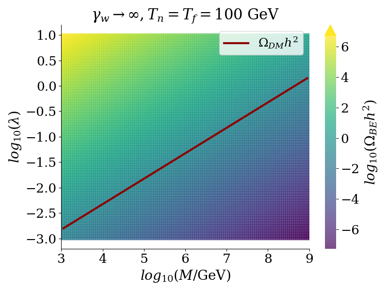
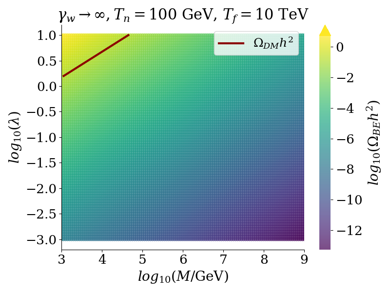
Figure 1: DM relic abundance for a renormalizable scalar-scalar interaction ($n=2$) in the ultra-relativistic limit for $v=200$ GeV and for $T_{\text{f}}=100$ GeV (upper panel) and $T_{\text{f}}=10$ TeV (lower panel). The red line stands for the points in agreement with the observational value, $\Omega_{\text{DM}}h^{2}=0.1200\pm 0.0012$ [46].

As seen in the upper panel of Figure 1, taking parameter values on the electroweak (EW) scale allows us to achieve a DM production in agreement with the observational value $\Omega_{\text{DM}}h^{2}=0.1200\pm 0.0012$ [46] for a wide range of couplings $\lambda$, which in addition allows for high masses of the DM candidate, typically forbidden in other DM production’s mechanisms [5]. Note, however, that this renormalizable scenario displays a strong dependence on the final temperature $T_{f}$. In particular, the higher this temperature, the lower the abundance. Thus, as $T_{f}$ increases, the parameter space in agreement with observations is reduced, as seen in the lower panel of Figure 1. Furthermore, for $T_{\text{f}}>100\,T_{n}$, we would not find parameter values in the presented range of $M$ and $\lambda$ for which production would be sufficient. Nonetheless, usually $T_{f}\gtrsim T_{n}$ [38, 39, 42]. Moreover, if the expansion is non-relativistic, the production becomes strongly suppressed, as seen in Eq. (21), being also insufficient. It is important to note that we are always considering values of the coupling constant at most of the order one, so the theory remains perturbative. Thus, the parameter space in the bottom panel of Figure 1 is even more constrained. Likewise, since we are interested in heavy DM candidates, we have not considered masses below the TeV scale.

III.2 Five-dimensional interaction ($n=3$)

The previous scenario constitutes the simplest realization of the BE mechanism allowing for the production of heavy DM candidates in agreement with observations. Nevertheless, the model is constrained to some extent by the bubble expansion velocity, while for final temperatures higher than the nucleation temperature the parameter space in agreement with observations is highly reduced. As we shall see in what follows, more general non-renormalizable interactions may actually enlarge the parameter space.

We start by considering the lowest-order non-renormalizable interaction in Eq. (2), namely $\mathcal{L}_{\text{int}}=\langle\Phi\rangle^{2}/\Lambda\,h\,\phi^{2}$, where we have conventionally reabsorbed the coupling constant $\lambda$ into the definition of the cutoff scale, which, for consistency, is taken to be the largest energy scale in the theory.

To compute the DM abundance, we carry out a process analogous to the previous case, calculating the matrix element $\mathcal{M}$ through Eq. (6), with $V(z)$ given again by (7). We obtain

$$\mathcal{M}=2i\lambda\left(\frac{v}{\Delta p_{z}}\right)^{2}\frac{1}{L_{w}\Lambda}\left[\frac{e^{2i\sigma}-1}{2\sigma}-i\right]\,.$$ (24)

and

$$\big{|}\mathcal{M}\big{|}^{2}=4\lambda^{2}\left(\frac{v}{\Delta p_{z}}\right)^{4}\left(\frac{1}{\Lambda L_{w}}\right)^{2}\left(\text{sinc}^{2}\sigma+1-2\,\text{sinc\,}2\sigma\,\right).$$ (25)

With this expression, we can now derive the decay probability via Eq. (10). Making the same assumptions and changes of variables as in the previous section, but ensuring also that the energy in the center of mass is lower than the cutoff scale so the effective theory holds, we obtain

$$\begin{split}\textit{P}=&\frac{\lambda^{2}}{24\pi^{2}}\left(\frac{v}{M}\right)^{4}\left(\frac{1}{\Lambda L_{w}}\right)^{2}\Theta(a)\Theta(b)\times\\ \bigg{[}&\frac{2}{35}\left(\frac{p_{0}}{M}\right)^{2}\big{(}1+\Theta(c)-2\Theta(d)\big{)}+\frac{\left(ML_{w}\right)^{2}}{3}\Theta(d)\bigg{]}\,,\end{split}$$ (26)

with $a=(p_{0}-2M)$, $b=(\Lambda^{2}-2p_{0}v)$, $c=(p_{0}-M^{2}L_{w})$ and $d=(p_{0}-2M^{2}L_{w})$. Note that in the considered heavy DM limit $M\gg v$ [28], we have $2M^{2}L_{w}>M^{2}L_{w}>2M$, which relates effectively the arguments of the Heaviside functions.

Given the probability (26) we can derive the DM density via Eq. (11) and with it the corresponding relic abundance through Eq. (13). Due to the complexity of the results, we present the complete expressions in Table 1, quoting here only the leading-order terms in $\gamma_{w}\gg 1$ and $\gamma_{w}\gg 2M^{2}/(vT_{n})$, namely

$${}^{3}n_{\phi}\simeq 8.5\cdot 10^{-4}\,\lambda^{2}\gamma_{w}\frac{T_{n}^{4}v^{5}}{\Lambda^{2}M^{4}}\,,$$ (27)

and

$${}^{3}\Omega_{\text{BE}}h^{2}\simeq 1.1\cdot 10^{8}\,\frac{\lambda^{2}\gamma_{w}}{g_{\star s}}\frac{T_{\text{n}}^{4}v^{4}}{T_{\text{f}}^{3}\Lambda^{2}M^{3}}\frac{v}{200\,\text{GeV}}\,,$$ (28)

or equivalently

$$\frac{{}^{3}\Omega_{\text{BE}}h^{2}}{{}^{2}\Omega_{\text{BE}}h^{2}}\simeq 4.1\cdot\gamma_{w}\cdot\frac{T_{\text{n}}v^{3}}{\Lambda^{2}M^{2}}\,.$$ (29)

Note that, unlike the result for $n=2$ in Eq. (23), these expressions depend explicitly on the Lorentz factor. This is due to the greater dependence of the decay probability on $p_{0}$, which follows itself from the stronger dependence of the interaction Lagrangian on the vev and its variation with $z$.

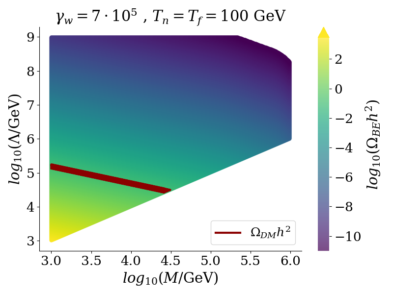
Figure 2: Same as for the upper panel in Figure 1 but for a non-renormalizable interaction with $n=3$ and $\gamma_{w}=7\cdot 10^{5}$.

The parameter space allowed by Eq. (29) for a FOPT at the EW scale is displayed in Figure 2. When studying the values in agreement with the observations, we use the complete expression for ${}^{3}\Omega_{\text{BE}}h^{2}$ presented in Table 1. The lower cut is for the limiting mass value consistent with the effective field theory description, $M=\Lambda$. In addition, in this case we can find agreement for velocities different from $v_{w}\rightarrow 1$, which was a constraint in the $n=2$ case, where an ultra-relativistic expansion was needed. Furthermore, thanks to the dependence on $\gamma_{w}$, the model holds for large values of the DM mass, while the impact of $T_{\text{f}}/T_{n}$ is reduced. Even so, the mass values that can be reached in the conditions shown in Figure 2 are of the order of the unitarity bound, not being able to exceed it.

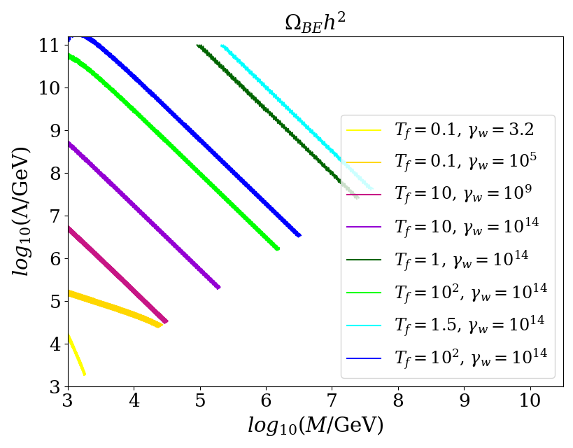
Figure 3: DM relic abundance for $n=3$ and different conditions. $T_{\text{f}}$ shown are in TeV. The yellow lines are for $v=200\,\text{GeV}$ and $T_{\text{n}}=100\,\text{GeV}$, as well as the purple/pink ones. The green lines are for $v=T_{\text{n}}=1\,\text{TeV}$ and the blue ones for $v=T_{\text{n}}=1.5\,\text{TeV}$.

It is interesting to consider values on scales other than the EW, and also different values of $T_{\text{f}}$, for which, in Figure 3, we represent only those values in agreement with observations. As shown in this plot, the novel dependencies on the Lorentz boost factor allow to compensate for the decrease of DM production caused by large values of the mass or final temperature. On the other hand, transitions in which the acquired vev is larger, as well as the nucleation temperature, allow for heavier DM candidates and a larger range of parameters in agreement with observations, especially for ultra-relativistic velocities.

Overall, the main difference between this non-renormalizable case and the one initially proposed in Ref. [28] and reviewed above ($n=2$) is that, even in the relativistic limit, the obtained DM relic abundance depends on the wall velocity, which allows for a wider range of DM masses.

III.3 Six-dimensional interaction ($n=4$)

In order to illustrate how the order of the non-dimensional interaction (2) affects the dependence of the DM abundance on the vev and the cutoff scale of the theory, we study in what follows the case $n=4$, namely $\mathcal{L}_{\text{int}}=\lambda\langle\Phi\rangle^{3}/\Lambda^{2}h,\phi^{2}$, where we have again reabsorbed the coupling constant $\lambda$ into the definition of the cutoff scale.

To obtain the abundance of DM relics, we follow the same procedure as before, making similar considerations when necessary. The resulting matrix element (6) takes now the form

$$\begin{split}\mathcal{M}=6\lambda\left(\frac{v}{\Delta p_{z}}\right)^{3}\left(\frac{1}{\Lambda L_{w}}\right)^{2}\left[\frac{1-e^{2i\sigma}}{2\sigma}+e^{2i\sigma}\left(\sigma+i\right)\right]\,,\end{split}$$ (30)

or equivalently

$$\begin{split}\big{|}\mathcal{M}\big{|}^{2}=36\lambda^{2}\left(\frac{v}{\Delta p_{z}}\right)^{6}\left(\frac{1}{\Lambda L_{w}}\right)^{4}\times\\ \left[\text{sinc}^{2}\sigma+1-2\,\text{sinc}\,2\sigma+\sigma^{2}(1-2\text{sinc}^{2}\sigma)\right]\,,\end{split}$$ (31)

Knowing this squared amplitude we can determine the decay probability via Eq. (10). To do so, we change coordinates to integrate over $x,k_{\perp}^{2},k_{0}^{\phi_{1}}$ and consider again the limit $p_{0}^{2}(1-x)^{2}\gg k_{\perp}^{2}+M^{2}$ and $p_{0}^{2}x^{2}\gg k_{\perp}^{2}+M^{2}$. The sought probability becomes

$$\begin{split}\mathcal{P}=\frac{3\lambda^{2}}{8\pi^{2}}\left(\frac{v}{M}\right)^{6}\left(\frac{1}{\Lambda L_{w}}\right)^{4}\Theta(a)\Theta(b)\bigg{[}\frac{8}{1155}\left(\frac{p_{0}}{M}\right)^{4}\\ \left(1+\Theta(c)-2\Theta(d)\right)+\frac{(p_{0}L_{w})^{2}}{70}\left(1-2\Theta(c)+\frac{4}{3}\Theta(d)\right)\bigg{]}\,,\end{split}$$ (32)

with $a=(p_{0}-2M)$, $b=(\Lambda^{2}-2p_{0}v)$, $c=(p_{0}-M^{2}L_{w})$ and $d=(p_{0}-2M^{2}L_{w})$. Recalling the heavy DM mass limit $M\gg v\simeq 1/L_{w}$, we have again the same relation between the arguments of the different Heaviside functions.

With the probability (32) at hand, we now derive the DM density, using Eq. (11), result that leads us directly to the DM relic abundance as shown in Eq. (13). Once again, the expressions for the number density and for the DM relic abundance are quite complex. Thus, we present the complete expression for the abundance in Table 1. At leading order in $\gamma_{w}\gg 1$ and $\gamma_{w}\gg 2M^{2}/(vT_{n})$, these quantities reduce to

$${}^{4}n_{\phi}\simeq 3.4\cdot 10^{-2}\,\lambda^{2}\gamma_{w}^{3}\frac{T_{n}^{6}v^{9}}{M^{8}\Lambda^{4}}\,,$$ (33)

and

$${}^{4}\Omega_{\text{BE}}h^{2}\simeq 4.2\cdot 10^{9}\,\frac{\lambda^{2}\gamma_{w}^{3}}{g_{\star s}}\frac{v^{8}T_{\text{n}}^{6}}{M^{7}\Lambda^{4}T_{\text{f}}^{3}}\frac{v}{200\,\text{GeV}}\,,$$ (34)

or equivalently

$$\frac{{}^{4}\Omega_{\text{BE}}h^{2}}{{}^{2}\Omega_{\text{BE}}h^{2}}\simeq 155.5\,\gamma_{w}^{3}\frac{T_{\text{n}}^{3}v^{7}}{\Lambda^{4}M^{6}}\,.$$ (35)

Note that, due to the larger dependence of the decay probability on $p_{0}$, these equations display an even larger dependence on $\gamma_{w}$ than the former case. The dependence on $T_{\text{n}}$ is given by the calculation of $n_{\phi}$ from the probability, which is different for each $n$, while the dependence on $T_{\text{f}}$ is always the same, since this appears when calculating the abundance via Eq. (13). This way, the higher is $n$, the greater is the dependence on $T_{\text{n}}$, being thus smaller the impact of $T_{\text{f}}>T_{\text{n}}$. On the other hand, the larger $n$ the greater the mass dependence, which reduces the possibility of having a heavy DM candidate. In spite of this and thanks to the dependence on $\gamma_{w}$, we can easily overcome this restriction with an ultra-relativistic wall, being this dependence larger the greater $n$.

${}^{3}\Omega_{\text{BE}}h^{2}=A^{\prime}\bigg{[}\frac{1}{(1-v_{w})^{4}}\left(f_{1}(2M/T_{n})+f_{1}(M^{2}/T_{n}v)-2f_{1}(2M^{2}/T_{n}v)\right)+\frac{1}{(1-v_{w})^{3}}\big{(}f_{2}(2M/T_{n})$

$\displaystyle+f_{2}(M^{2}/T_{n}v)-2f_{2}(2M^{2}/T_{n}v)\big{)}\bigg{]}+B^{\prime}\left(\frac{2M^{2}}{v(1-v_{w})}\frac{\gamma_{w}}{T_{\text{n}}}+\frac{(2-v_{w})}{(1-v_{w})^{2}}\right)e^{-\frac{\gamma_{w}2M^{2}(1-v_{w})}{T_{\text{n}}v}}$

with $\displaystyle A^{\prime}=\frac{1.54\cdot 10^{6}\lambda^{2}}{\gamma_{w}^{6}v_{w}g_{\star s}}\frac{T_{\text{n}}^{5}}{T_{\text{f}}^{3}\Lambda^{2}}\frac{v^{5}}{M^{5}}v_{200}$   and   $\displaystyle B^{\prime}=\frac{8.98\cdot 10^{6}\lambda^{2}}{\gamma_{w}^{4}v_{w}g_{\star s}}\frac{T_{\text{n}}^{3}}{T_{\text{f}}^{3}}\frac{v^{3}}{M\Lambda^{2}}v_{200}$

${}^{4}\Omega_{\text{BE}}h^{2}=A\bigg{[}\frac{1}{(1-v_{w})^{4}}\left(f_{1}(2M/T_{n})-2f_{1}(M^{2}/T_{n}v)+\frac{4}{3}f_{1}(2M^{2}/T_{n}v)\right)+\frac{1}{(1-v_{w})^{3}}\big{(}f_{2}(2M/T_{n})$

$\displaystyle-2f_{2}(M^{2}/T_{n}v)+\frac{4}{3}f_{2}(2M^{2}/T_{n}v)\big{)}\bigg{]}+B\bigg{[}\frac{1}{(1-v_{w})^{6}}\big{(}f_{3}(2M/T_{n})+f_{3}(M^{2}/T_{n}v)$

$\displaystyle-2f_{3}(2M^{2}/T_{n}v)\big{)}+\frac{1}{(1-v_{w})^{5}}\left(f_{4}(2M/T_{n})+f_{4}(M^{2}/T_{n}v)-2f_{4}(2M^{2}/T_{n}v)\right)\bigg{]}$

with $\displaystyle A=\frac{3.47\cdot 10^{6}\lambda^{2}}{g_{\star s}v_{w}\gamma_{w}^{6}}\frac{T_{\text{n}}^{5}}{M^{5}}\frac{v^{4}}{\Lambda^{4}}\frac{v^{3}}{T_{\text{f}}^{3}}v_{200}$  and   $\displaystyle B=\frac{1.42\cdot 10^{6}\lambda^{2}}{g_{\star s}\gamma_{w}^{8}v_{w}}\frac{T_{\text{n}}^{7}}{\Lambda^{4}T_{\text{f}}^{3}}\frac{v^{9}}{M^{9}}v_{200}$

$\displaystyle f_{n}(x)=\left[\sum_{i=0}^{j}{\left(\gamma_{w}(1-v_{w})x\right)^{i}\frac{j!}{i!}}\right]e^{-\gamma_{w}(1-v_{w})x}$

$\displaystyle\text{with }j=3\text{ for }n=1\text{, }j=2\text{ for }n=2\text{, }j=5\text{ for }n=3\text{ and }j=4\text{ for }n=4.$

Table 1: Complete expressions of the DM relic abundance for $n=3$ and $n=4$. The quantity $v_{200}$ stands for the vev on the non-symmetric side of the wall normalized by $200$ GeV, $v_{200}=v/(200\,\text{GeV})$.

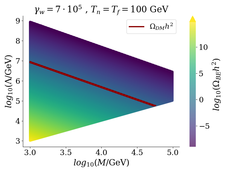
Figure 4: Same as for the upper panel in Figure 1 but for a non-renormalizable interaction with $n=4$ and $\gamma_{w}=7\cdot 10^{5}$.

As shown in Figure 4, and under the same conditions as previous cases, the parameter space in agreement with observations for a FOPT transition at the electroweak scale allows a wider range of values for both $\Lambda$ and $M$. However, the masses are of the order of the unitarity bound, not being able to exceed it under the conditions presented. Once again, the lower cut in Figure 4 stands for $M=\Lambda$.

As before, it is interesting to consider the effect of the final temperature as well as other values of the vev and the nucleation temperature. For this purpose, we make use of ultra-relativistic velocities, studying how the dependence in $\gamma_{w}$ compensates for large values of $M$, allowing again superheavy candidates. The values in agreement with observations following the complete expressions in Table 1 are shown in Figure 5, where we consider the same cases discussed in the previous subsection. Again, we verify how an ultra-relativistic bubble-wall velocity allows a wide range of possibilities for the parameters. Likewise, we have again that for higher values of $v$ and $T_{\text{n}}$ the DM production is higher. Moreover, we can see how, in comparison with the case $n=3$, this model allows for larger masses and a wider range of $\Lambda$ values, due to the greater dependence in $\gamma_{w}$ and $T_{\text{n}}$. In addition, the larger range for $\Lambda$ shows that the model is valid up to a larger scale of energies.

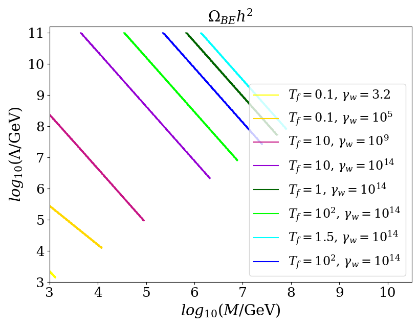
Figure 5: Same as for Figure 3 but for $n=4$.

So far, we have observed a general behavior for the abundance as $n$ increases. First, the dependence on $T_{n}$ increases, favoring production and decreasing the negative impact of a final temperature $T_{\text{f}}\gg T_{n}$, which can occur in certain regimes. However, the weight of $M$ in the denominator also increases, which a priori reduces the possibility of obtaining heavy DM candidates. Nonetheless, in the non-renormalizable cases we find an increasing dependence on $\gamma_{w}$, which allows large values of the mass for relativistic velocities (even above the unitarity bound), as well as a validity of the model up to a higher energy scales. Therefore, the larger $n$ is, the greater the range of possible FOPTs compatible with the BE mechanism. Moreover, all these tendencies can be expected to continue for larger $n$ so there will come a point where the dependence on $\gamma_{w}$ will be such that the ultra-relativistic regime will be excluded, since it will always lead to overproduction.

IV GWs SIGNAL

One of the most interesting features of our DM production via expanding bubbles is the associated generation of sizable GWs, as this signal could eventually serve as indirect evidence for it.

GWs in FOPT have been a widely studied topic in recent years, being their current understanding essentially due to hydrodynamic and scalar field simulations [43, 47, 48, 49, 50]. In the scenarios under consideration, we can identify a priori three possible contributions to the gravitational wave spectrum: the scalar field contribution due to collisions between bubbles, the sound waves contribution due to sound waves generated by the energy transfer from $h$ to the plasma, and the turbulent contribution due to nonlinear effects in the turbulent motion of the plasma. However, due to the large uncertainties it presents and since it is expected to be subdominant [43], we will not consider the turbulent contribution. To parametrize the relative weight of the two remaining contributions, we introduce the effective parameters,

$$k_{\text{\rm wall}}=\frac{E_{\text{\rm wall}}}{E_{\text{total}}}\,,\hskip 28.45274ptk_{\text{fluid}}=1-k_{\text{\rm wall}}\,,$$ (36)

governing respectively the energy distribution between the wall motion and the plasma excitation, with $E_{wall}$ the wall kinetic energy.

Regarding the velocity of bubbles, we can distinguish two regimes: the terminal velocity regime, in which the friction is sufficient to slow down the bubble wall so it reaches a constant velocity, and the runaway regime, in which the energy released is such that the wall continues to accelerate until collision, reaching ultra-relativistic velocities. In the former case, only sound waves contribute to the GW production since, once the terminal velocity is reached, the portion of the energy stored in the wall starts to decrease as the inverse of the bubble radius, so that $k_{\text{fluid}}=1$. On the other hand, in the latter case we have $k_{\text{\rm wall}}=1-\alpha_{\infty}/\alpha$, with $\alpha_{\infty}$ the value of $\alpha$ from which we are in the runaway regime [51]. Thus, both the scalar and sound waves contributions are a priori important in this case.

The scalar field or bubble collision GW contribution following from numerical simulations takes the form [48]

$$\frac{\textit{d}\Omega_{\phi}h^{2}}{\textit{d}ln(f)}=4.7\cdot 10^{-8}\left(\frac{100}{g_{*s}}\right)^{1/3}(H_{\text{f}}R_{*})^{2}\left(\frac{k_{\text{\rm wall}}\alpha}{1+\alpha}\right)^{2}S_{\text{\rm wall}},$$ (37)

with $g_{*s}$ evaluated at the time of GWs generation, $H_{\text{f}}$ the Hubble parameter at the final temperature and

$$R_{*}=\frac{(8\pi)^{1/3}v_{w}}{\beta}\,,$$ (38)

the size of the bubble at the collision. Here $S_{\text{\rm wall}}$ stands for the numerically-fitted spectral function

$$S_{\text{\rm wall}}=\frac{(a+b)^{c}f_{p}^{b}f^{a}}{(bf_{p}^{\frac{a+b}{c}}+af^{\frac{a+b}{c}})^{c}}\,,$$ (39)

with $a=3$, $b=1.51$, $c=2.18$, $f$ the frequency and

$$f_{p}=5.28\cdot 10^{-4}\frac{T_{\text{f}}}{100\,\text{GeV}}\left(\frac{g_{*}}{100}\right)^{1/6}\frac{1}{2\pi R_{*}H_{\text{f}}}\,,$$ (40)

the peak frequency.

On the other hand, the sound waves GW contribution in the prescription of Ref. [49] reads

$$\frac{\textit{d}\Omega_{sw}h^{2}}{\textit{d}ln(f)}=\left\{\begin{array}[]{cr}0.678h^{2}F_{\text{\text{sw}}}G\tilde{\Omega}_{\text{sw}}C(s),&\text{if}\quad\frac{H_{\text{f}}R_{*}}{K^{1/2}}>1\,;\\ 0.678h^{2}F_{\text{sw}}\bar{G}\tilde{\Omega}_{\text{sw}}C(s),&\text{if}\quad\frac{H_{\text{f}}R_{*}}{K^{1/2}}<1\,.\end{array}\right.\,.$$ (41)

Here, we have $F_{\text{sw}}=3.57\cdot 10^{-5}(100/g_{*})^{1/3}$, $G=K^{2}H_{\text{f}}R_{*}/c_{s}$ and $\bar{G}=K^{3/2}(H_{\text{f}}R_{*}/c_{s})^{2}$, with $c_{s}$ the speed of sound and

$$K\approx\frac{3}{4}\frac{k_{\text{sw}}\alpha}{1+\alpha},\quad k_{\text{sw}}=k_{\text{fluid}}\frac{\alpha}{0.73+0.083\sqrt{\alpha}+\alpha}\,,$$ (42)

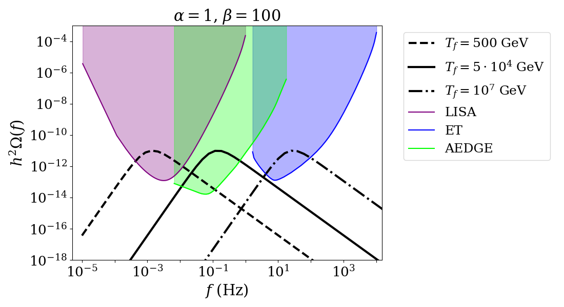
Figure 6: GW spectra for fixed values of $\alpha,\beta$ in the runaway regime. We are always taking $\alpha_{\infty}=0.001$. The presented values of $\beta$ are in units of $H_{\text{f}}$. LISA [33], ET [32] and AEDGE [34] sensitivity curves are also presented.

where, for the case of runaway regime, we have to substitute $\alpha$ with $\alpha_{\infty}$. The spectral shape $C(s)$ is numerically found to be

$$C(s)=s^{3}\left(\frac{7}{4+3s^{2}}\right)^{7/2}\,,\quad\quad s\equiv\frac{f}{f_{p}}\,,$$ (43)

with peak frequency

$$f_{p}\simeq 26\cdot 10^{-6}\frac{1}{H_{\text{f}}R_{*}}\frac{z_{p}}{10}\frac{T_{\text{f}}}{100\,\text{GeV}}\left(\frac{g_{*}}{100}\right)^{1/6}\text{Hz}\,,$$ (44)

and peak angular frequency $z_{p}=(kR_{*})_{\text{max}}$ generally around 10. Last, numerical simulations give $\tilde{\Omega}_{\text{sw}}\approx 10^{-2}$ [49].

The GW spectra resulting from the above expressions is shown in Figure 6 for $\alpha_{\infty}=0.001$, typical values of $\alpha$ and $\beta$, and different values of the final FOPT temperature $T_{f}$, which as given by Eq. (44) depends linearly on the peak frequency $f_{p}$. As shown in this plot, a FOPT with final temperature above the EW scale ($100\,\text{GeV}$) and below $T_{f}=10^{7}\,\text{GeV}$ is well within the reach of future GWs experiments. Note also that, although we have concentrated in a runaway regime, the spectra for terminal velocity regime would be also very similar.

V CONCLUSIONS AND OUTLOOK

Cosmological first-order phase transitions provide a natural way of producing massive dark matter particles in the very early Universe. In this paper, we have considered the Bubble Expansion mechanism for the production of scalar DM candidates, focusing on non-renormalizable interactions between the dark sector and the field undergoing the transition and remaining otherwise agnostic about the effective potential responsible for it. Our results complement previous studies in the literature dealing with renormalizable scalar interactions [35], Proca-like couplings [36] and non-renormalizable operators mediating the production of heavy fermions and gauge bosons [37].

Contrary to what happens in renormalizable scenarios, the number density of created particles and the associated DM relic abundance in the ultra-relativistic limit were shown to depend explicitly on the Lorentz boost factor $\gamma_{w}$, being this dependence more relevant the larger the dimension of the interaction term under consideration. This enables observational compatibility for sizable cutoff scales and a wide range of DM masses and transition temperatures typically excluded in renormalizable scenarios. The obtained results display also a good tolerance to differences between the final transition temperature $T_{f}$ and the nucleation temperature $T_{n}$, in clear contrast with renormalizable settings, where the viable parameter space is significantly reduced for $T_{\text{f}}>T_{\text{n}}$. Interestingly enough, for final temperatures in the range $100\,{\rm GeV}\lesssim T_{f}\lesssim 10^{7}\,\text{GeV}$, the GW spectrum following from the collision of bubbles generated during the FOPT and the sound waves induced in the plasma is also within the reach of future GWs observatories, such as the Einstein Telescope (ET) [32], the Laser Interferometer Space Antenna (LISA) [33] or the Atomic Experiment for DM and Gravity Exploration in space (AEDGE) [34].

Although we have implicitly assumed all the DM in the Universe to be produced by a BE mechanism, its generation might potentially occur along with other DM production channels, modifying with it the parameter space in agreement with observations. For instance, final transition temperatures exceeding the mass of scalar DM candidates coupled to the thermal bath could result in additional Freeze-Out production, with Freeze-In contributions becoming likely relevant in the opposite regime [37]. Also, one could consider DM production from bubble collisions [20], although this mechanism is typically subdominant as compared to the one discussed here [28, 37]. Finally, once the DM is produced, its evolution will depend on how it interacts with the thermal bath, mainly through the transition field. A priori, one could envisage a free streaming regime in which the scattering is out of equilibrium and the velocities of the DM particles are not modified, and a cold DM regime in which the scattering slows down the produced particles until they reach non-relativistic velocities [37]. However, the latter case is usually not relevant for DM scalar particles generated via renormalizable interactions [35], this being the output also expected for weaker interactions such as those considered in this paper.

VI Acknowledgments

JL acknowledges the support of the Institute of Particle and Cosmos Physics through the “M.Sc. grants IPARCOS-UCM/2023”. JR is supported by a Ramón y Cajal contract of the Spanish Ministry of Science and Innovation with Ref. RYC2020-028870-I. This work was supported by the project PID2022-139841NB-I00 of MICIU/AEI/10.13039/501100011033 and FEDER, UE.

References

- Cirelli et al. [2024] M. Cirelli, A. Strumia, and J. Zupan, Dark Matter, (2024), arXiv:2406.01705 [hep-ph] .
- Srednicki et al. [1988] M. Srednicki, R. Watkins, and K. A. Olive, Calculations of Relic Densities in the Early Universe, Nucl. Phys. B 310, 693 (1988).
- Gondolo and Gelmini [1991] P. Gondolo and G. Gelmini, Cosmic abundances of stable particles: Improved analysis, Nuclear Physics B 360, 145 (1991).
- Griest and Seckel [1991] K. Griest and D. Seckel, Three exceptions in the calculation of relic abundances, Phys. Rev. D 43, 3191 (1991).
- Griest and Kamionkowski [1990] K. Griest and M. Kamionkowski, Unitarity Limits on the Mass and Radius of Dark Matter Particles, Phys. Rev. Lett. 64, 615 (1990).
- Baldes and Petraki [2017] I. Baldes and K. Petraki, Asymmetric thermal-relic dark matter: Sommerfeld-enhanced freeze-out, annihilation signals and unitarity bounds, JCAP 09, 028, arXiv:1703.00478 [hep-ph] .
- Smirnov and Beacom [2019] J. Smirnov and J. F. Beacom, TeV-Scale Thermal WIMPs: Unitarity and its Consequences, Phys. Rev. D 100, 043029 (2019), arXiv:1904.11503 [hep-ph] .
- McDonald [2002] J. McDonald, Thermally generated gauge singlet scalars as selfinteracting dark matter, Phys. Rev. Lett. 88, 091304 (2002), arXiv:hep-ph/0106249 .
- Choi and Roszkowski [2005] K.-Y. Choi and L. Roszkowski, E-WIMPs, AIP Conf. Proc. 805, 30 (2005), arXiv:hep-ph/0511003 .
- Kusenko [2006] A. Kusenko, Sterile neutrinos, dark matter, and the pulsar velocities in models with a Higgs singlet, Phys. Rev. Lett. 97, 241301 (2006), arXiv:hep-ph/0609081 .
- Petraki and Kusenko [2008] K. Petraki and A. Kusenko, Dark-matter sterile neutrinos in models with a gauge singlet in the Higgs sector, Phys. Rev. D 77, 065014 (2008), arXiv:0711.4646 [hep-ph] .
- Hall et al. [2010] L. J. Hall, K. Jedamzik, J. March-Russell, and S. M. West, Freeze-In Production of FIMP Dark Matter, JHEP 03, 080, arXiv:0911.1120 [hep-ph] .
- Bernal et al. [2017] N. Bernal, M. Heikinheimo, T. Tenkanen, K. Tuominen, and V. Vaskonen, The Dawn of FIMP Dark Matter: A Review of Models and Constraints, Int. J. Mod. Phys. A 32, 1730023 (2017), arXiv:1706.07442 [hep-ph] .
- Elahi et al. [2015] F. Elahi, C. Kolda, and J. Unwin, UltraViolet Freeze-in, JHEP 03, 048, arXiv:1410.6157 [hep-ph] .
- Bernal et al. [2020a] N. Bernal, J. Rubio, and H. Veermäe, Boosting Ultraviolet Freeze-in in NO Models, JCAP 06, 047, arXiv:2004.13706 [hep-ph] .
- Bernal et al. [2020b] N. Bernal, J. Rubio, and H. Veermäe, UV Freeze-in in Starobinsky Inflation, JCAP 10, 021, arXiv:2006.02442 [hep-ph] .
- Murayama and Shu [2010] H. Murayama and J. Shu, Topological Dark Matter, Phys. Lett. B 686, 162 (2010), arXiv:0905.1720 [hep-ph] .
- Khoze and Ro [2014] V. V. Khoze and G. Ro, Dark matter monopoles, vectors and photons, JHEP 10, 061, arXiv:1406.2291 [hep-ph] .
- Bai et al. [2020] Y. Bai, M. Korwar, and N. Orlofsky, Electroweak-Symmetric Dark Monopoles from Preheating, JHEP 07, 167, arXiv:2005.00503 [hep-ph] .
- Falkowski and No [2013] A. Falkowski and J. M. No, Non-thermal Dark Matter Production from the Electroweak Phase Transition: Multi-TeV WIMPs and ’Baby-Zillas’, JHEP 02, 034, arXiv:1211.5615 [hep-ph] .
- Freese and Winkler [2023] K. Freese and M. W. Winkler, Dark matter and gravitational waves from a dark big bang, Phys. Rev. D 107, 083522 (2023), arXiv:2302.11579 [astro-ph.CO] .
- Mansour and Shakya [2023] H. Mansour and B. Shakya, On Particle Production from Phase Transition Bubbles, (2023), arXiv:2308.13070 [hep-ph] .
- Shakya [2023] B. Shakya, Aspects of Particle Production from Bubble Dynamics at a First Order Phase Transition, (2023), arXiv:2308.16224 [hep-ph] .
- Giudice et al. [2024] G. F. Giudice, H. M. Lee, A. Pomarol, and B. Shakya, Nonthermal Heavy Dark Matter from a First-Order Phase Transition, (2024), arXiv:2403.03252 [hep-ph] .
- Baldes et al. [2024] I. Baldes, M. Dichtl, Y. Gouttenoire, and F. Sala, Particle shells from relativistic bubble walls, (2024), arXiv:2403.05615 [hep-ph] .
- Bodeker and Moore [2017a] D. Bodeker and G. D. Moore, Electroweak Bubble Wall Speed Limit, JCAP 05, 025, arXiv:1703.08215 [hep-ph] .
- Azatov and Vanvlasselaer [2021] A. Azatov and M. Vanvlasselaer, Bubble wall velocity: heavy physics effects, JCAP 01, 058, arXiv:2010.02590 [hep-ph] .
- Azatov et al. [2021] A. Azatov, M. Vanvlasselaer, and W. Yin, Dark Matter production from relativistic bubble walls, JHEP 03, 288, arXiv:2101.05721 [hep-ph] .
- Hindmarsh et al. [2021] M. Hindmarsh et al., Phase transitions in the early universe, SciPost Phys. Lect. Notes 24, 1 (2021), arXiv:2008.09136 [astro-ph.CO] .
- Caprini and Figueroa [2018] C. Caprini and D. G. Figueroa, Cosmological Backgrounds of Gravitational Waves, Class. Quant. Grav. 35, 163001 (2018), arXiv:1801.04268 [astro-ph.CO] .
- Steinhardt [1982] P. J. Steinhardt, Relativistic detonation waves and bubble growth in false vacuum decay, Phys. Rev. D 25, 2074 (1982).
- Punturo et al. [2010] M. Punturo et al., The Einstein Telescope: A third-generation gravitational wave observatory, Class. Quant. Grav. 27, 194002 (2010).
- LISA Collaboration et al. [2017] P. LISA Collaboration, Amaro-Seoane et al., Laser Interferometer Space Antenna, . (2017), arXiv:1702.00786 [astro-ph.IM] .
- El-Neaj et al. [2020] Y. A. El-Neaj et al. (AEDGE), AEDGE: Atomic Experiment for Dark Matter and Gravity Exploration in Space, EPJ Quant. Technol. 7, 6 (2020), arXiv:1908.00802 [gr-qc] .
- Baldes et al. [2023] I. Baldes, Y. Gouttenoire, and F. Sala, Hot and heavy dark matter from a weak scale phase transition, SciPost Phys. 14, 033 (2023), arXiv:2207.05096 [hep-ph] .
- Ai et al. [2024] W.-Y. Ai, M. Fairbairn, K. Mimasu, and T. You, Non-thermal production of heavy vector dark matter from relativistic bubble walls, (2024), arXiv:2406.20051 [hep-ph] .
- Azatov et al. [2024] A. Azatov, X. Nagels, M. Vanvlasselaer, and W. Yin, Populating secluded dark sector with ultra-relativistic bubbles, (2024), arXiv:2406.12554 [hep-ph] .
- Caprini et al. [2016] C. Caprini et al., Science with the space-based interferometer eLISA. II: Gravitational waves from cosmological phase transitions, JCAP 04, 001, arXiv:1512.06239 [astro-ph.CO] .
- Ellis et al. [2019a] J. Ellis, M. Lewicki, and J. M. No, On the Maximal Strength of a First-Order Electroweak Phase Transition and its Gravitational Wave Signal, JCAP 04, 003, arXiv:1809.08242 [hep-ph] .
- Vanvlasselaer [2022] M. E. A. Vanvlasselaer, Dynamics of phase transitions in the early universe and cosmological consequences, Ph.D. thesis, SISSA, Trieste (2022).
- Breitbach [2018] M. Breitbach, Gravitational Waves from Cosmological Phase Transitions, Master’s thesis, Mainz U. (2018), arXiv:2204.09661 [astro-ph.CO] .
- Ellis et al. [2019b] J. Ellis, M. Lewicki, J. M. No, and V. Vaskonen, Gravitational wave energy budget in strongly supercooled phase transitions, JCAP 06, 024, arXiv:1903.09642 [hep-ph] .
- Caprini et al. [2020] C. Caprini et al., Detecting gravitational waves from cosmological phase transitions with LISA: an update, JCAP 03, 024, arXiv:1910.13125 [astro-ph.CO] .
- Bodeker and Moore [2017b] D. Bodeker and G. D. Moore, Electroweak Bubble Wall Speed Limit, JCAP 05, 025, arXiv:1703.08215 [hep-ph] .
- Husdal [2016] L. Husdal, On Effective Degrees of Freedom in the Early Universe, Galaxies 4, 78 (2016), arXiv:1609.04979 [astro-ph.CO] .
- Aghanim et al. [2020] N. Aghanim et al. (Planck), Planck 2018 results. VI. Cosmological parameters, Astron. Astrophys. 641, A6 (2020), [Erratum: Astron.Astrophys. 652, C4 (2021)], arXiv:1807.06209 [astro-ph.CO] .
- Gould et al. [2021] O. Gould, S. Sukuvaara, and D. Weir, Vacuum bubble collisions: From microphysics to gravitational waves, Phys. Rev. D 104, 075039 (2021), arXiv:2107.05657 [astro-ph.CO] .
- Cutting et al. [2018] D. Cutting, M. Hindmarsh, and D. J. Weir, Gravitational waves from vacuum first-order phase transitions: from the envelope to the lattice, Phys. Rev. D 97, 123513 (2018), arXiv:1802.05712 [astro-ph.CO] .
- Hindmarsh et al. [2017] M. Hindmarsh, S. J. Huber, K. Rummukainen, and D. J. Weir, Shape of the acoustic gravitational wave power spectrum from a first order phase transition, Phys. Rev. D 96, 103520 (2017), [Erratum: Phys.Rev.D 101, 089902 (2020)], arXiv:1704.05871 [astro-ph.CO] .
- Hindmarsh et al. [2014] M. Hindmarsh, S. J. Huber, K. Rummukainen, and D. J. Weir, Gravitational waves from the sound of a first order phase transition, Phys. Rev. Lett. 112, 041301 (2014), arXiv:1304.2433 [hep-ph] .
- Espinosa et al. [2010] J. R. Espinosa, T. Konstandin, J. M. No, and G. Servant, Energy Budget of Cosmological First-order Phase Transitions, JCAP 06, 028, arXiv:1004.4187 [hep-ph] .