Effects of primordial fluctuations on relic neutrino simulations

Abstract

After decoupling, relic neutrinos traverse the evolving gravitational imhomogeneities along their trajectories. Once they turn non-relativistic, this results in a significant amplification of the anisotropies in the cosmic neutrino background (C$\nu$B). Past studies have reconstructed the phase-space distribution of relic neutrinos from the local distribution of matter (accounting for the Milky Way halo and the surrounding large-scale structures), but have neglected the C$\nu$B anisotropies in the initial conditions of neutrino trajectories. Using our previously developed N-1-body simulation framework, we show that including these primordial fluctuations in the initial conditions can be important, as it produces similar effects on the abundance and anisotropies of the C$\nu$B as the inclusion of large-scale structures beyond the Milky Way halo. Interpretability of data from future C$\nu$B observatories like PTOLEMY therefore depends on correctly modelling these effects.

GitHub: Our jax-accelerated simulation code can be found here.

1 Introduction

A fundamental prediction of the concordance cosmological model is the presence of a cosmic background of relic neutrinos (C$\nu$B), formed when they decoupled from the primordial plasma only one second after the Big Bang. While there is strong indirect evidence of the C$\nu$B around the Big Bang Nucleosynthesis (BBN) [1, 2] and the Cosmic Microwave Background (CMB) [3, 4] eras, little is known about their properties. In particular, their absolute mass scale and mass ordering are still unknown, but are projected to be measured in the coming years (see e.g. [5]). Their background phase-space distribution is assumed to be of the Fermi-Dirac type [6, 7, 8] as per theoretical expectations, although there exist only weak cosmological bounds on relic neutrino statistics [9, 10].

The direct detection of the C$\nu$B in a laboratory setting also remains a huge challenge. Future experiments such as PTOLEMY [11] aim to detect the C$\nu$B via neutrino capture on $\beta$-decaying nuclei, in particular tritium. The event rate in these experiments is proportional to the local number density of relic neutrinos, which is expected to be larger than the cosmological average due to gravitational effects in the vicinity of the Earth. If the tritium targets are polarized, this would possibly allow the measurement of C$\nu$B anisotropies [12], which are also expected to be influenced by the local gravitational environment. Hence, to understand the prospects of these future experiments, previous works have investigated gravitational clustering of relic neutrinos via linear perturbation theory [13, 14, 15, 16] or N-body or N-1-body simulation frameworks [17, 18, 19, 20, 21, 22].

However, all these works have so far assumed a perfectly homogenous and isotropic Fermi-Dirac distribution for neutrinos right before the onset of non-linear structure formation. In practice, we expect there to be some non-negligible fluctuations in the phase-space distribution which are induced by the primordial fluctuations in the matter fields. Using linear theory, it was shown in [23] that such primordial fluctuations lead to anisotropies in the C$\nu$B temperature that can grow up to ${\sim}10\%$ of the mean C$\nu$B temperature of $T_{\nu,0}\sim 1.95$ K.

The C$\nu$B anisotropies exhibit a very rich phenomenology that presents several important differences compared to those of the CMB. To illustrate this, we show a schematic diagram of our past lightcone including neutrinos in Figure 1. The horizontal direction represents comoving distance and the vertical direction conformal time. In addition to our spacetime point at the tip of the cone (at $z_{0}=0$), we show three other constant-time hypersurfaces at $z_{\mathrm{sim}}=4$ (the time boundary of our simulations, as explained later), $z_{\mathrm{CMB}}\approx 10^{3}$ (roughly the time of photon decoupling) and $z_{\mathrm{C}\nu\mathrm{B}}\approx 10^{9}$ (roughly the time of neutrino decoupling).

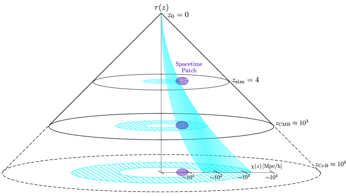
Figure 1: Schematic diagram of our past lightcone, extrapolated until the time of neutrino decoupling. The cyan band roughly represents $0.05\,\mathrm{eV}$ neutrinos with comoving momenta in the range of about $[0.01,10]$ times the present C$\nu$B temperature. Note that the spacings and areas are not to scale; the figure is merely aimed to be a helpful visualization.

The lightlike worldline is depicted with the solid black lines at a $45^{\circ}$ angle, and we extended this lightcone beyond the CMB for illustrative purposes with the dashed black lines. The cyan band approximately represents $0.05\,\mathrm{eV}$ neutrinos with comoving momenta in the range of $0.01$ to $10$ times the present C$\nu$B temperature. At neutrino decoupling they are ultra-relativistic, with an angle of almost $45^{\circ}$, then slow down due to the cosmic expansion, which corresponds to a progressively increasing change of the angle as they become more and more non-relativistic at low redshifts. The hatched cyan shell elements represent the domains of space which relic neutrinos of this momentum band traverse. The fact that the C$\nu$B originates from a last-scattering surface closer to us than the CMB [24, 25, 26], where the distance is determined by the neutrino momentum, is clearly visible in this diagram: the CMB photons travelled $\sim 10^{4}~{}\mathrm{Mpc}$, whereas the majority of relic neutrinos travelled $\sim 10^{3}~{}\mathrm{Mpc}$ (in comoving units). This means that neutrinos with different masses, or equivalently, neutrinos of the same mass but with different momenta pass through the same “spacetime patch” (illustrated in purple) at different times. As a result, the temperature anisotropies differ between neutrino momenta (and masses), as they are affected by different evolving gravitational potentials at distinct times. The framework developed in [23] computes these C$\nu$B anisotropies.

In our previous work [22], we constructed a numerical simulation framework based on the approach of [20], to compute the local C$\nu$B density as well as its anisotropies. This was done by initializing relic neutrinos at Earth and reconstructing their trajectories through the local gravitational environment by running the simulations backwards to a time, where the neutrino phase-space was assumed to be Fermi-Dirac. Liouville’s theorem maps this phase-space to the (unknown) one today, allowing the moments of the distribution like e.g. the number density to be computed. Even though our simulation space in that study only contained dark matter (DM) halos resembling the Milky Way (MW), without the large-scale structure (LLS), we uncovered effects not seen with previous analytical treatments: the neutrinos could be “diffused” by DM particles along their trajectories, producing anti-correlations between the neutrino number densities and the projected DM content along the line-of-sight. We speculated that the inclusion of LSS might enhance this effect, depending on how much DM structure a neutrino of a given momentum traverses.

In this work, we describe an extension to this framework to partially account for the effects of LSS $-$ motivated by the previous discussion and the most recent work of C$\nu$B clustering [21]. In that latest study they employed both full N-body and N-1-body simulation techniques to study relic neutrino clustering, fully including LSS inside their $1\,\mathrm{Gpc}^{3}$ simulation volume. Amongst other things, they showed that distant DM structures can be anti-correlated with local neutrino fluctuations in the same direction on the sky, with the effect being more evident for smaller neutrino masses which traverse greater distances. The net effect of including LSS appears to always contribute positively to the number density, with the fractional contribution to the total density being dependent on the neutrino mass. To make precise predictions about the local C$\nu$B properties it thus seems crucial to include the LSS of the Universe. We show that when modifying the boundary conditions of our simulation by including anisotropic phase-space distributions from linear primordial fluctuations, we recover some of the effects that one would obtain by fully modeling the LSS within the N-body simulation domain.

The remainder of this work is structured to reflect the order of execution to arrive at the results. The methodology (section 2) is divided into three parts: how we reconstruct the neutrino trajectories and compute the number densities (section 2.1), how we compute the C$\nu$B anisotropies (section 2.2), and how we build the new boundary conditions for the neutrino trajectories based on these anisotropies (section 2.3). The results are then presented in section 3 and we disuss and conclude in section 4.

2 Methods

In this section we give an overview of our simulation framework, for which more details can be found in [22]. We then show how to compute the C$\nu$B temperature anisotropies with the framework developed in [23] and describe how to change the boundary conditions for our simulations accordingly.

2.1 C$\nu$B simulations

Our simulations reconstruct relic neutrino trajectories, which are governed by Hamilton’s equations of motion

$$\vec{q}_{j}=am_{\nu}\vec{x}_{j}^{\prime},\quad\vec{q}\mkern 2.0mu\vphantom{q}_{j}^{\prime}=-am_{\nu}\frac{\partial\Phi(\vec{x},t)}{\partial\vec{x}_{j}},$$ (2.1)

where $\vec{q}_{j}$ is the comoving momentum of the $j$-th neutrino and $\vec{x}_{j}$ its position. The prime notation of these quantities denotes the derivative with respect to conformal time. The scale factor $a$ accounts for the cosmic expansion, and any effect due to non-linear structure formation enters via the gravitational potentials $\Phi$ at position $\vec{x}$ and time $t$. These potentials are formed by DM halos selected from the TangoSIDM project [33, 34] and have masses consistent with the estimated Milky-Way mass using the Gaia data [35, 36, 37, 38], whose values are within the range of $M_{200}=(0.6\mbox{--}2.0)\times 10^{12}\,\mathrm{M_{\odot}}$. Here, we use 27 such halos whose merger and accretion history is represented by how the DM particles comprising the halo are distributed at various redshifts. The DM distribution at a redshift is referred to as a snapshot, and we use 25 of them between redshifts $0$ and $4$. We run the simulation backwards in time, which implies that the neutrinos are initiated in a cell with a distance from the halo center akin to the distance of Earth to the MW Galactic center. They are then aimed in different directions corresponding to the pixels of a healpy allsky map with a resolution of $\mathrm{Nside}=8$ (768 pixels). There are multiple cells fitting this distance criterion, but we showed in [22] that choosing a different starting cell does not change the overall results much. We upgraded our previous code using the jax programming paradigm [39] to accelerate the simulations, as well as to solve the equations of motion with the jax-compatible diffrax library. This allowed us to both increase precision and decrease computation time. We found that simulating 1000 neutrinos for each direction in the sky with this methodology was sufficient. The momenta are spaced logarithmically in the range $[0.01~{}T_{\nu,0},~{}400~{}T_{\nu,0}]$. We used a 128 CPU core cluster node with 224 GB memory to run the simulations, resulting in a runtime of $\mathcal{O}(1)$ minutes for a single halo.

Such simulations allow us to find the final positions $\vec{x}_{j}(z_{\rm sim})$ and momenta $\vec{q}_{j}(z_{\rm sim})$ of the neutrinos at the last redshift of our simulations, $z_{\rm sim}$. Liouville’s theorem states that the phase-space density is conserved along particle trajectories, so this allows us to compute the present values of the phase-space as

$$f(\vec{x}_{\oplus},\vec{q}_{j}(0),0)=f_{\rm sim}(\vec{x}_{j}(z_{\rm sim}),\vec{q}_{j}(z_{\rm sim}),z_{\rm sim}),$$ (2.2)

where $\vec{x}_{\oplus}$ is the starting coordinate of all neutrinos (i.e. the position of Earth) and $f_{\rm sim}$ represents the initial phase-space distribution of the neutrinos at $z_{\rm sim}$. The local number density per degree of freedom is then computed as

$$n_{\nu}=\int\frac{d^{3}\vec{q}_{0}}{(2\pi)^{3}}\,f(\vec{x}_{\oplus},\vec{q}_{0},0),$$ (2.3)

where the integral should be understood as a sum over the momenta $\vec{q}_{j}(0)$ of all simulated neutrinos.

2.2 Angular power spectrum

In our previous study [22] we had assumed a Fermi-Dirac distribution to describe the state of the C$\nu$B at the last redshift of our simulations, i.e. $f_{\rm sim}=f_{\rm FD}$ in eq. (2.2). We now go over the equations from cosmological perturbation theory necessary to compute the anisotropies in the C$\nu$B temperature, which are induced by the evolving gravitational inhomogeneities along the trajectories of the relic neutrinos. This will ultimately give us a perturbed phase-space distribution, $f_{\Delta}$, which serves as a proxy for the effects from LSS. For this, we adapted the line-of-sight method from [23]. We refer the reader to that study for details omitted in this section.

We start by introducing a perturbation $\Psi$ in the Fermi-Dirac distribution for neutrinos to get the perturbed distribution

$$f(\vec{x},q,\hat{n},\tau)=f_{\rm FD}(q)(1+\Psi(\vec{x},q,\hat{n},\tau))=\frac{1}{e^{\frac{q}{T_{\nu,0}}}+1}(1+\Psi(\vec{x},q,\hat{n},\tau)),$$ (2.4)

where the vector $\hat{n}$ represents the direction of comoving momenta. If we now write the left-hand side in terms of a fractional temperature perturbation $\Delta$,

$$f_{\Delta}(q)=\left(e^{\frac{q}{T_{\nu,0}(1+\Delta)}}+1\right)^{-1}$$ (2.5)

and expand this to linear order, we can express $\Delta$ in terms of $\Psi$ as

$$\Delta=-\left(\frac{d\ln f_{\rm FD}}{d\ln q}\right)^{-1}\Psi.$$ (2.6)

Note that the neutrino temperature perturbation $\Delta$ depends not only on space and time, but also on momenta, meaning that the perturbed phase-space $f_{\Delta}$ acquires spectral distortions. From now on, we will only display the momentum dependence for simplicity. To eliminate the dependence on direction it is customary to switch to Fourier space and expand $\tilde{\Psi}$ in Legendre multipoles; the resulting neutrino perturbations per multipole, $\tilde{\Psi}_{\ell}$, obey a Boltzmann hierarchy of equations that can be solved numerically with Boltzmann solvers like CLASS [40]. Then, from $\tilde{\Psi}_{\ell}$ one can obtain the associated temperature perturbations $\tilde{\Delta}_{\ell}$ via eq. (2.6). These in turn can be used to get the angular power spectrum with

$$C_{\ell}(q)=4\pi T_{\nu,0}^{2}A_{s}\int d\ln k\tilde{\Delta}_{\ell}^{2}(q),$$ (2.7)

where $A_{s}$ is the primordial power spectrum amplitude.

The so-called line-of-sight method allows for a quick calculation of $\tilde{\Delta}_{\ell}(q)$ up to a very large $\ell_{\rm max}$ without having to solve a Boltzmann hierarchy of $(\ell_{\rm max}+1)$ equations. More precisely, this method expresses $\tilde{\Delta}_{\ell}(q)$ as an integral from neutrino decoupling ($\tau_{\mathrm{dec}}$) to the present day ($\tau_{0})$, namely

$$\tilde{\Delta}_{\ell}(q)=\frac{1}{2}\phi_{\rm dec}j_{\ell}(k\chi(z_{\rm dec}))+\int_{\tau_{\rm dec}}^{\tau_{0}}d\tau\left\{2\left(\frac{am_{\nu}}{q}\right)^{2}(aH)\phi+\left[2+\left(\frac{am_{\nu}}{q}\right)^{2}\right]\partial_{\tau}\phi\right\}j_{\ell}(k\chi(z_{\tau})).$$ (2.8)

In this equation, we see the spherical Bessel functions of the first kind $j_{\ell}$, the neutrino mass $m_{\nu}$ and the Hubble parameter $H$. The second term represents the amplification of anisotropies due to the evolving gravitational potential $\phi$ (in the conformal Newtonian gauge) encountered by neutrinos during their non-relativistic phase, while the first term with $\phi_{\mathrm{dec}}$ captures the anisotropies at neutrino decoupling. Finally, the Bessel functions depend on the comoving distance traveled by massive neutrinos from an initial redshift $z_{i}$ to a final redshift $z_{f}$ (with $z_{i}>z_{f}$) as given by

$$\chi(z_{i},q)=\int_{z_{f}}^{z_{i}}\frac{dz}{H(z)}\frac{q}{\sqrt{q^{2}+m_{\nu}^{2}/(1+z)^{2}}}.$$ (2.9)

Note the dependence of $\chi(z_{i},q)$ on the ratio $m_{\nu}/q$, as we illustrated in Figure 1. The method also allows the momentum-averaged angular power spectrum to be expressed as

$$C_{\ell}=4\pi T_{\nu,0}^{2}A_{s}\int d\ln k\left(\int dq\,\tilde{\Delta}_{\ell}(q)\,\frac{2}{3\zeta(3)T^{3}_{0}}\,\frac{q^{2}}{e^{\frac{q}{T_{0}}}+1}\right)^{2}.$$ (2.10)

2.3 Boundary conditions

We can use the expressions for the angular power spectrum of the previous section to construct more accurate boundary conditions for our simulations. Technically, the spatial boundary varies for each neutrino: the ones initialized with a high momentum ($q_{\mathrm{high}}$) end up further away from Earth than those starting with a low momentum ($q_{\mathrm{low}}$). We therefore have to find the correct value of $\Delta$ for each neutrino. For the following explanation, it is again helpful to turn to an illustration.

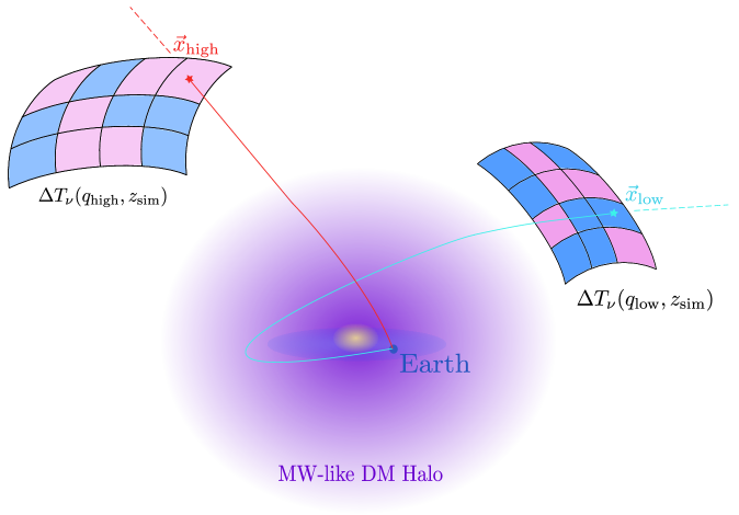
Figure 2: Schematic illustration of the temperature fluctuation surfaces (colored grids) at the last redshift of our simulations of $z_{\mathrm{sim}}=4$ for fast- ($q_{\mathrm{high}}$) and slow-moving ($q_{\mathrm{low}}$) neutrinos (see text for more details concerning the connection between the surfaces and neutrino trajectories). The Milky Way disc and bulge, as depicted by the blue and yellow oval shapes, are for visualization purposes only, since our simulations do not include baryonic components.

Figure 2 schematically shows patches of two different temperature fluctuation surfaces depicted by the curved pink and blue colored grids. These illustrate possible temperature fluctuation patterns arising from the angular power spectrum in eq. (2.7) for the two different neutrino momenta. The red and cyan curves exemplify trajectories of neutrinos with $q_{\mathrm{high}}$ and $q_{\mathrm{low}}$, respectively. The last positions of these neutrinos (i.e. at $z_{\rm sim}$) are marked with $\vec{x}_{\mathrm{high}}$ and $\vec{x}_{\mathrm{low}}$, where they have momenta $q_{\rm high}^{z_{\rm sim}}$ and $q_{\rm low}^{z_{\rm sim}}$, respectively.

Let us now rewind time to neutrino decoupling and follow two specific “newly-released” neutrinos with momenta $q^{\mathrm{C}\nu\mathrm{B}}_{\mathrm{high}}$ and $q^{\mathrm{C}\nu\mathrm{B}}_{\mathrm{low}}$, which will end up at these positions. Due to the influence of the primordial gravitational potential $\phi$, these momenta will evolve until reaching values $q_{\rm high}^{z_{\rm sim}}$ and $q_{\rm low}^{z_{\rm sim}}$, which characterize a linearly perturbed phase-space according to the formalism described in section 2.2. So to get the correct value of $\Delta$ for each neutrino at their boundary, we need to: i) plug their corresponding momentum at $z_{\rm sim}$ into eq. (2.7), ii) generate the corresponding all-sky temperature anisotropy maps, and iii) select the pixel corresponding to their last position. Then, eq. (2.5) yields the corresponding phase-space value, and we just set $f_{\rm sim}=f_{\Delta}$ to compute the number density with eq. (2.2) and eq. (2.3). In this way we account for the effects of a random linear LSS configuration from neutrino decoupling at $z_{\mathrm{C}\nu\mathrm{B}}\approx 10^{9}$ until the last redshift of our time-reversed simulations at $z_{\rm sim}=4$. Notice that to get the approriate temperature fluctuation skymaps at $z_{\rm sim}$ we need to cut off the time integrals in eq. (2.8). The computation of $\tilde{\Delta}_{\ell}(q)$ via this equation is characterized by two independent terms: a term proportional to the gravitational potential at neutrino decoupling ($\phi_{\mathrm{dec}}$) and a term with an integral over time. The first term also depends on the comoving distance through the Bessel function, and hence also involves an integral over time. By cutting off these time integrals at a specific time prior to today, $\tau_{\mathrm{cut}}$ (or $z_{\mathrm{cut}}$), we effectively stop the evolution of the primordial temperature anisotropies at that time. An extra multiplicative factor of $(1+z_{\mathrm{cut}})^{2}$ is also needed in eq. (2.7) to obtain the correct value of the monopole temperature at $z_{\mathrm{cut}}$, since $T\propto a^{-1}$. This procedure gives us the angular power spectrum at that higher redshift, $C_{\ell}(z_{\mathrm{cut}})$, from which we can produce temperature anisotropy skymaps and ultimatly obtain the perturbed phase-space values, $f_{\Delta}(z_{\rm cut})$.

To highlight the neccessity to include these more realistic boundary conditions for our simulations, we show the evolution of the neutrino energy density contrast $\delta_{\nu}$ for $0.01$, $0.05$, $0.1$ and $0.2$ eV neutrinos in figure 3. To get an approximate estimate of $\delta_{\nu}(z)$, we generated skymaps of the temperature perturbations at different redshifts, as realised by eq. (2.10) with the $z_{\rm cut}$-technique described above.

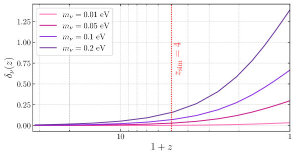
Figure 3: Approximate neutrino energy density contrast as a function of redshift for different neutrino masses of $0.01$, $0.05$, $0.1$ and $0.2$ eV (see text for details on the calculation of this quantity). The last redshift of our simulation of $z_{\rm sim}=4$ is marked with the red dotted line. The overdensities around that time can already reach ${\sim 20\%}$, highlighting the neccessity to account for these deviations from an isotropic and homogeneous phase-space distribution.

Then, to obtain $\delta T_{\nu}$ we took the mean of the 2 extremes around the monopole temperature (one positive and one negative), and converted this into a density contrast using $\delta_{\nu}(z)\sim 3\frac{\delta T_{\nu}}{T_{\nu}}(z)$, which holds for non-relativistic neutrinos. From figure 3, we see that the assumption of a Fermi-Dirac distribution at our simulation boundary redshift ($z_{\mathrm{sim}}=4$) is not appropriate, as the density contrasts can already reach up to ${\sim}20\%$ for certain neutrino masses. We will show below that this has consequences for the number densities as obtained with our simulation framework, and that by accounting for these initial density perturbations, we can partly mimic the effects one would obtain when fully including LSS (i.e. structures beyond the MW Galaxy) inside the simulation domain.

3 Results

We now show the changes to the local number density and anistropies of the C$\nu$B when using a perturbed phase-space distribution instead of the isotropic Fermi-Dirac distribution as the boundary condition of our simulation. The results representing the former case are obtained when setting $f_{\rm sim}=f_{\Delta}$ in eq. (2.2), whereas setting $f_{\rm sim}=f_{\rm FD}$ represents the latter case.

3.1 Local number density

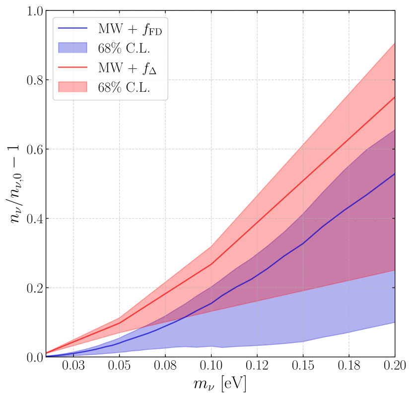
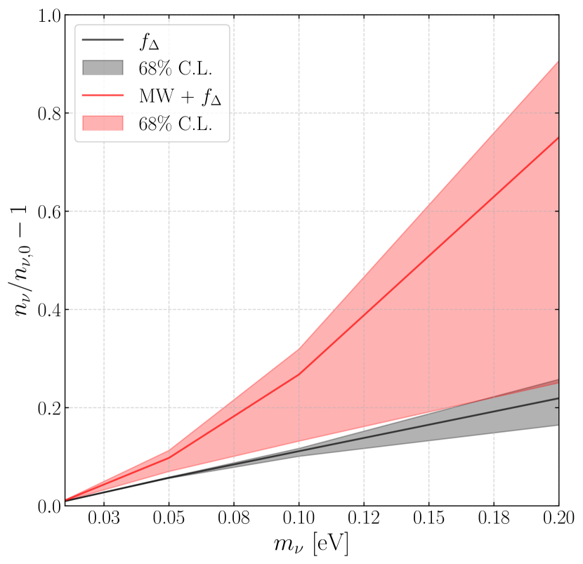
Figure 4: Neutrino clustering factors as a function of neutrino mass. The shaded areas represent the dispersion among the 27 different MW-like DM halos used in our simulations. Left panel: The blue band is obtained when using an isotropic Fermi-Dirac ($f_{\mathrm{FD}}$) as the boundary condition, and the red band results when using a perturbed phase-space ($f_{\Delta}$). Right panel: The contribution solely due to the effects of linear LSS (i.e. the primordial perturbations) is represented by the black band, and the red band is again shown for comparison.

Figure 4 displays the C$\nu$B number densities normalized to the cosmological average value (i.e. ${\sim}56\,\mathrm{cm}^{-3}$ per mass eigenstate and per helicity) for a range of neutrino masses. The two panels show three different curves, where the spread is due to the different DM distributions of the 27 halos. The solid lines show the median and the shaded areas represent 68% coverage bands. In blue we show the simulations using $f_{\mathrm{FD}}$ as the boundary condition, whereas red (appearing in both panels) represent the simulations using $f_{\Delta}$. The two different types of simulations effectively let us quantify the additional effect that comes from linear LSS on top of the MW gravitational potential. To emphasize this aspect, in black we additionally show the contribution coming from the primordial perturbations only, which was simply obtained by subtracting the blue band from the red band. We see that switching from $f_{\mathrm{FD}}$ to $f_{\Delta}$ increases the number density on average for all neutrino masses, the effect being actually larger for smaller neutrino masses. Our results seem to agree well with Figure 3 in [21], where the authors show the individual contribution of LSS included in their simulations. The change to more realistic boundary conditions thus has meaningful consequences and should be included for a N-1-body simulation framework such as ours.

3.2 Anisotropies

The final point of interest concerns the C$\nu$B anisotropies, which are also affected by the change in boundary conditions. We first visualize the effects by showing a comparison between skymaps for $0.1\,{\rm eV}$ neutrinos in figure 5, where the left map was generated using $f_{\mathrm{FD}}$ and the right map with a random realisation of $f_{\Delta}$. One noticeable change is the slight widening of the range of the under- and overdensity values for the pixels. Even though the minimal value decreases and larger patches depict underdense regions in the sky, the overall effect of the primordial fluctuations is still net positive for the number densities, as we saw in Figure 4. To illustrate the impact for lighter neutrinos, in figure 9 of appendix A we show a skymap for a neutrino mass of $0.01\,{\rm eV}$.

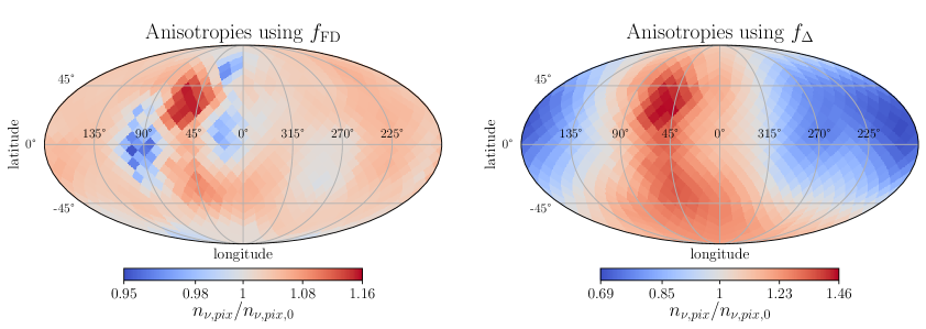
Figure 5: Comparison of C$\nu$B anisotropy sky maps for $0.1\,{\rm eV}$ neutrinos, when applying the two different boundary conditions: using the isotropic Fermi-Dirac ($f_{\mathrm{FD}}$) generates the left panel, while using the perturbed phase-space ($f_{\Delta}$) generates the right panel. The densities are normalized to the cosmological average value on a per pixel basis.

Another change is the appearance of features on large angles. This becomes more apparent in the corresponding angular power spectra, that we show in Figure 6 for $0.1\,{\rm eV}$ (left panel) and $0.01\,{\rm eV}$ (right panel) neutrinos. The blue (red) band in this figure denotes the spectrum of the sky map generated using $f_{\mathrm{FD}}$ ($f_{\Delta}$). More specifically, we used 10 realizations of $f_{\Delta}$ for each halo. This figure therefore shows the combined uncertainty associated to the MW-like DM halos as well as the linear LSS. In figure 7 of appendix A, we seperately show the effects of these two sources of uncertainty, and conclude that the different realizations of $f_{\Delta}$ dominate the uncertainties. For both neutrino masses, the power for the first few multipoles can increase up to an order of magnitude when including the effects of primordial fluctuations. The power for higher multipoles are only affected for the lighter neutrinos. This reflects the fact that the lighter neutrinos traverse larger distances before reaching Earth, therefore having more time to pick up the effects on smaller scales than the heavier neutrinos.

In [20], it was found that most of the gravitational clustering happens at very low redshifts of $z\lesssim 0.5$, and we tested that the same holds true for our framework. Moreover, we have found that lowering the simulation boundary redshift to about $z_{\rm sim}\approx 0.5$, and hence allowing more time for the primordial overdensities to grow while still simulating the most important clustering regime with our N-1-body framework, does not yield a significant increase in power at low-$\ell$. We show this explicitly in figure 8 of appendix A. This is in line with the findings of [23] where it was shown that the greatest contribution of primordial fluctuations to the low-$\ell$ part of the C$\nu$B spectra comes from scales below ${\sim}100\,{\rm Mpc}$ for $0.05\,{\rm eV}$ neutrinos (and hence even smaller scales for more massive neutrinos), i.e. at very low redshifts.

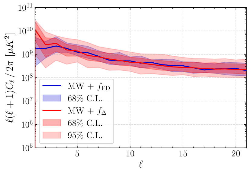
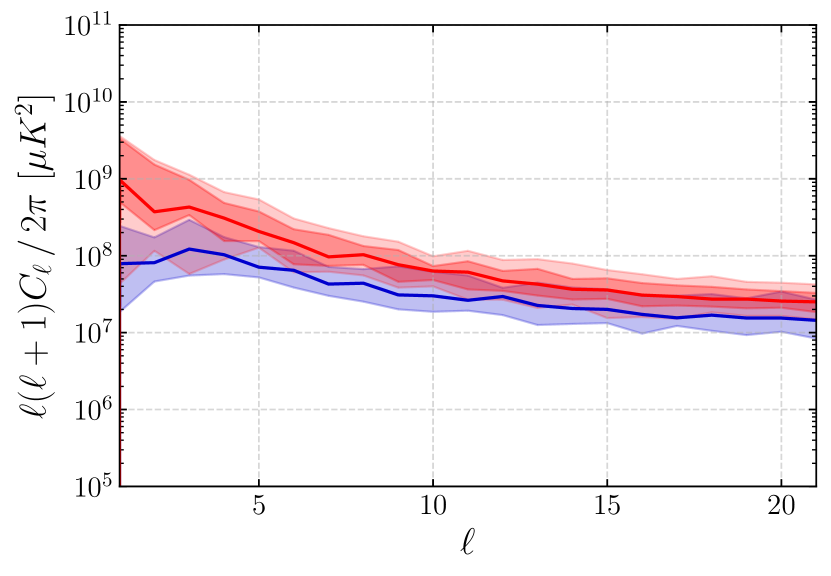
Figure 6: Angular power spectra of the C$\nu$B anisotropies for $0.1\,{\rm eV}$ (left panel) and $0.01\,{\rm eV}$ (right panel) neutrinos. The bands in blue result from using an isotropic Fermi-Dirac ($f_{\rm FD}$) as the boundary conditions, whereas a perturbed phase-space ($f_{\Delta}$) was used to produce the red bands. The solid curves represent the median values of our DM halo sample, whereas the dark and light shaded areas indicate 68% and 95% coverage bands, respectively.

4 Discussion & Conclusions

In this last section we discuss some advantages and shortcomings of this work and additional points of interest regarding the results. We end by summarizing our main findings.

Pros and cons.

A shortcoming of modelling LSS with linear theory based on power spectra is that it is unconstrained. The resulting, and effectively random large scale temperature fluctuations may not exhibit the pattern realized in nature. So we can only make statements about average quantities and discuss global trends, as done in this work. An advantage of this simulation framework is its speed and flexibility: number densities can quickly be compared for different phase-space or DM distributions. Future constraints on these two quantities may make this simulation approach more useful.

Comparison to state-of-the-art.

Our results differ from those of the latest N-body simulation of [21], especially the magnitude and shape of the anisotropy power spectra. The median power on large scales in figure 6 is about an order of magnitude lower compared to the results of that study, whereas our power spectra drop off less quickly on smaller scales. Both are explicable by looking at how our methodology differs: we resolve scales of the DM halos down to ${\sim}2.5\,{\rm Mpc}$, but don’t model the effects of LSS in the non-linear regime for redshift $\lesssim 0.5$. The result is more power on smaller scales but less on the largest scales.

Importance of primordial fluctuations.

The idea of introducing small phase-space density fluctuations at the boundary of the simulation to account for any clustering that took place since the onset of structure formation has been mentioned in [20]. However, based on their observation that their results were independent from pushing back the redshift of their simulation boundary, the authors concluded that any clustering since the onset of structure formation outside their simulation domain could be safely neglected. As we showed in e.g. figure 4, the contribution of these seemingly miniscule fluctuations do contribute to C$\nu$B properties, and hence should not be ignored in such a simulation framework.

Future detectability.

A direct detection of the C$\nu$B via experiments like PTOLEMY, and its proposed successors using polarized tritium that may be sensitive to the incoming direction of the relic neutrinos [12], may be possible in the future. However, it is expected that the initially poor angular resolution of such directional C$\nu$B experiments will only be able to pick up the variations on large scales, but as these scales would be sensitive to changes in the C$\nu$B temperature, that quantity could be measurable [23]. Since the primordial fluctuations investigated in this work mainly affect the largest scales, they would need to be included in the modeling if an inference of the C$\nu$B temperature is to be attempted.

In this work we extended our C$\nu$B simulator developed in [22] that only included local DM halos resembling the MW in terms of virial mass. By using cosmological perturbation theory to compute the evolution of C$\nu$B temperature anisotropies, we could generate a perturbed phase-space distribution for the neutrinos at our simulation boundary, giving more realistic initial conditions than the usual isotropic Fermi-Dirac distribution. The key points to be taken away from this work are as follows.

• The redshift boundary of an N-1-body simulation framework such as the one used here matters, as the neutrino overdensities can grow in magnitude such that they have to be modelled and accounted for accurately. We show how the neutrino density constrast evolves over time in figure 3.

• The inclusion of LSS always contributes positively to the local C$\nu$B number density. Linear LSS alone can account already for almost up to $20\%$ of the clustering factors for the higher neutrino masses around $0.2$ eV, as can be seen in the right panel of figure 4.

• The lowest multipoles of the C$\nu$B angular power spectra increase in power up to an order of magnitude when using the perturbed phase-space distribution $f_{\Delta}$ at the simulation boundary, as can be seen in figure 6. Since the values of $f_{\Delta}$ are generated in a random fashion from the $C_{\ell}$, we also show the spread due to different $f_{\Delta}$ realisations in figure 7, where it is visible that the increase in power can vary up to an order of magnitude.

• The dominant contribution to the lower multipoles of the C$\nu$B angular power spectrum come from the structure the neutrinos traverse in their last few $\mathcal{O}(10)\text{--}\mathcal{O}(100)\,{\rm Mpc}$. As this happens at very low redshifts of $\lesssim 0.5$, lowering the redshift of our simulation boundary did not increase that power significantly, which is visible when comparing figure 8 to figure 7.

The main motivation of this study was to find an effective way to include the effects of LSS in an N-1-body simulation framework. Figure 6 shows that the methodology proposed here is able to partially do so: the difference in power on low multipoles can be as small as half an order of magnitude compared to the results from state-of-the-art N-body simulations [21], for some of our DM halos. The power towards smaller scales does not drop off as quickly, due to the nature of our highly-resolved N-1-body simulation space on MW scales. Therefore, it offers be a viable alternative to simulate and test physical models involving the C$\nu$B in a computationally less expensive way.

Appendix A Supplementary figures

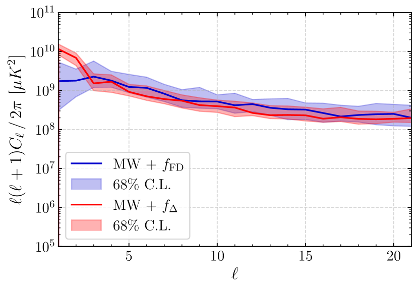
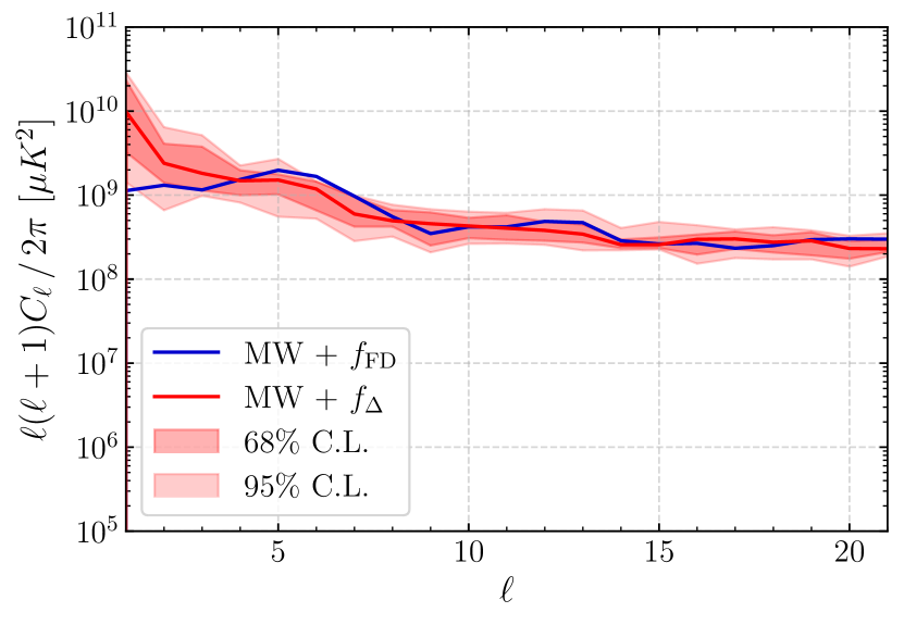
Figure 7: Angular power spectra of the C$\nu$B anisotropies for $0.1\,{\rm eV}$ neutrinos, with the same color code as in figure 6. Left panel: The dispersion is obtained from our whole halo sample and one realization of $f_{\Delta}$. Right panel: The dispersion is obtained from 10 different realizations of $f_{\Delta}$ and one halo. This shows that the uncertainty is dominated by the $f_{\Delta}$’s, since the associated effects can vary up to an order of magnitude at low-$\ell$.

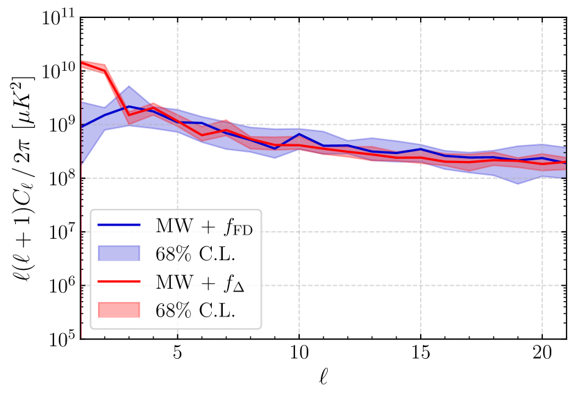
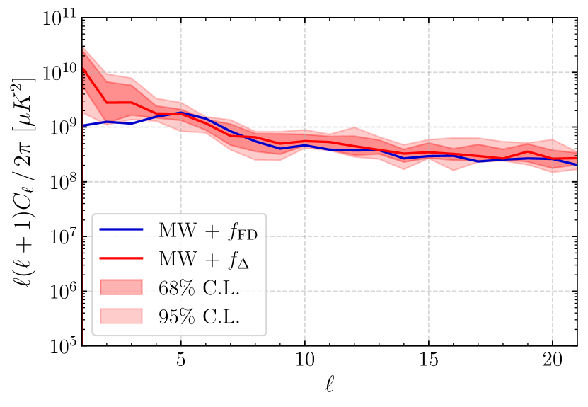
Figure 8: Angular power spectra of the C$\nu$B anisotropies for $0.1\,{\rm eV}$ neutrinos, when lowering the redshift of the simulation boundary from $z_{\rm sim}=4$ to $z_{\rm sim}=0.5$. The meaning of the uncertainty bands is the same as in figure 7.

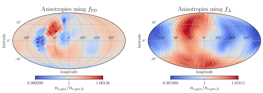
Figure 9: Comparison of C$\nu$B anisotropy sky maps as in figure 5, but for $0.01\,{\rm eV}$ neutrinos.

References

- [1] O. Pisanti, G. Mangano, G. Miele and P. Mazzella, Primordial Deuterium after LUNA: concordances and error budget, JCAP 04 (2021) 020 [2011.11537].
- [2] B.D. Fields, K.A. Olive, T.-H. Yeh and C. Young, Big-Bang Nucleosynthesis after Planck, JCAP 03 (2020) 010 [1912.01132].
- [3] B. Follin, L. Knox, M. Millea and Z. Pan, First Detection of the Acoustic Oscillation Phase Shift Expected from the Cosmic Neutrino Background, Phys. Rev. Lett. 115 (2015) 091301 [1503.07863].
- [4] D.D. Baumann, F. Beutler, R. Flauger, D.R. Green, A. Slosar, M. Vargas-Magaña et al., First constraint on the neutrino-induced phase shift in the spectrum of baryon acoustic oscillations, Nature Phys. 15 (2019) 465 [1803.10741].
- [5] M. Gerbino et al., Synergy between cosmological and laboratory searches in neutrino physics, Phys. Dark Univ. 42 (2023) 101333 [2203.07377].
- [6] E.W. Kolb and M.S. Turner, The Early Universe, vol. 69 (1990), 10.1201/9780429492860.
- [7] J. Lesgourgues, G. Mangano, G. Miele and S. Pastor, Neutrino Cosmology, Cambridge University Press (2, 2013).
- [8] D. Baumann, Cosmology, Cambridge University Press (7, 2022), 10.1017/9781108937092.
- [9] P.F. de Salas, S. Gariazzo, M. Laveder, S. Pastor, O. Pisanti and N. Truong, Cosmological bounds on neutrino statistics, JCAP 03 (2018) 050 [1802.04639].
- [10] J. Alvey, M. Escudero and N. Sabti, What can CMB observations tell us about the neutrino distribution function?, JCAP 02 (2022) 037 [2111.12726].
- [11] PTOLEMY collaboration, Neutrino physics with the PTOLEMY project: active neutrino properties and the light sterile case, JCAP 07 (2019) 047 [1902.05508].
- [12] M. Lisanti, B.R. Safdi and C.G. Tully, Measuring Anisotropies in the Cosmic Neutrino Background, Phys. Rev. D 90 (2014) 073006 [1407.0393].
- [13] S. Singh and C.-P. Ma, Neutrino clustering in cold dark matter halos : Implications for ultrahigh-energy cosmic rays, Phys. Rev. D 67 (2003) 023506 [astro-ph/0208419].
- [14] J. Alvey, M. Escudero, N. Sabti and T. Schwetz, Cosmic neutrino background detection in large-neutrino-mass cosmologies, Phys. Rev. D 105 (2022) 063501 [2111.14870].
- [15] E.B. Holm, I.M. Oldengott and S. Zentarra, Local clustering of relic neutrinos with kinetic field theory, 2305.13379.
- [16] E.B. Holm, S. Zentarra and I.M. Oldengott, Local clustering of relic neutrinos: Comparison of kinetic field theory and the Vlasov equation, 2404.11295.
- [17] A. Ringwald and Y.Y.Y. Wong, Gravitational clustering of relic neutrinos and implications for their detection, JCAP 12 (2004) 005 [hep-ph/0408241].
- [18] P.F. de Salas, S. Gariazzo, J. Lesgourgues and S. Pastor, Calculation of the local density of relic neutrinos, JCAP 09 (2017) 034 [1706.09850].
- [19] J. Zhang and X. Zhang, Gravitational clustering of cosmic relic neutrinos in the Milky Way, Nature Commun. 9 (2018) 1833 [1712.01153].
- [20] P. Mertsch, G. Parimbelli, P.F. de Salas, S. Gariazzo, J. Lesgourgues and S. Pastor, Neutrino clustering in the Milky Way and beyond, JCAP 01 (2020) 015 [1910.13388].
- [21] W. Elbers, C.S. Frenk, A. Jenkins, B. Li, S. Pascoli, J. Jasche et al., Where shadows lie: reconstruction of anisotropies in the neutrino sky, JCAP 10 (2023) 010 [2307.03191].
- [22] F. Zimmer, C.A. Correa and S. Ando, Influence of local structure on relic neutrino abundances and anisotropies, JCAP 11 (2023) 038 [2306.16444].
- [23] C.G. Tully and G. Zhang, Multi-messenger astrophysics with the cosmic neutrino background, JCAP 06 (2021) 053 [2103.01274].
- [24] G.S. Bisnovatyi-Kogan and Z.F. Seidov, The Neutrino Horizon of the Universe, Soviet Astronomy 27 (1983) 125.
- [25] G.S. Bisnovatyi-Kogan and Z.F. Seidov, The Neutrino in the Friedmann Universe - Non-Zero Rest-Mass Effects, Astrophysics and Space Science 102 (1984) 131.
- [26] S. Dodelson and M. Vesterinen, Cosmic Neutrino Last Scattering Surface, Phys. Rev. Lett. 103 (2009) 171301 [0907.2887].
- [27] J.Y.-Y. Lin and G. Holder, Gravitational Lensing of the Cosmic Neutrino Background, JCAP 04 (2020) 054 [1910.03550].
- [28] R.J. Michney and R.R. Caldwell, Anisotropy of the Cosmic Neutrino Background, JCAP 01 (2007) 014 [astro-ph/0608303].
- [29] S. Hannestad and J. Brandbyge, The Cosmic Neutrino Background Anisotropy - Linear Theory, JCAP 03 (2010) 020 [0910.4578].
- [30] S. Betts et al., Development of a Relic Neutrino Detection Experiment at PTOLEMY: Princeton Tritium Observatory for Light, Early-Universe, Massive-Neutrino Yield, in Snowmass 2013: Snowmass on the Mississippi, 7, 2013 [1307.4738].
- [31] A.J. Long, C. Lunardini and E. Sabancilar, Detecting non-relativistic cosmic neutrinos by capture on tritium: phenomenology and physics potential, JCAP 08 (2014) 038 [1405.7654].
- [32] C.G. Tully and G. Zhang, Impact of Warm Dark Matter on the Cosmic Neutrino Background Anisotropies, Universe 8 (2022) 118 [2201.01888].
- [33] C.A. Correa, M. Schaller, S. Ploeckinger, N. Anau Montel, C. Weniger and S. Ando, TangoSIDM: Tantalizing models of Self-Interacting Dark Matter, 2206.11298.
- [34] C. Correa, M. Schaller, J. Schaye, S. Ploeckinger, J. Borrow and Y. Bahe, TangoSIDM Project: Is the Stellar Mass Tully-Fisher relation consistent with SIDM?, 2403.09186.
- [35] E.V. Karukes, M. Benito, F. Iocco, R. Trotta and A. Geringer-Sameth, A robust estimate of the Milky Way mass from rotation curve data, JCAP 05 (2020) 033 [1912.04296].
- [36] L. Posti and A. Helmi, Mass and shape of the Milky Way’s dark matter halo with globular clusters from Gaia and Hubble, AAP 621 (2019) A56 [1805.01408].
- [37] G. Eadie and M. Jurić, The Cumulative Mass Profile of the Milky Way as Determined by Globular Cluster Kinematics from Gaia DR2, Astrophys. J. 875 (2019) 159 [1810.10036].
- [38] T.K. Fritz, G. Battaglia, M.S. Pawlowski, N. Kallivayalil, R. van der Marel, S.T. Sohn et al., Gaia DR2 proper motions of dwarf galaxies within 420 kpc. Orbits, Milky Way mass, tidal influences, planar alignments, and group infall, AAP 619 (2018) A103 [1805.00908].
- [39] J. Bradbury, R. Frostig, P. Hawkins, M.J. Johnson, C. Leary, D. Maclaurin et al., JAX: composable transformations of Python+NumPy programs, 2018.
- [40] D. Blas, J. Lesgourgues and T. Tram, The Cosmic Linear Anisotropy Solving System (CLASS) II: Approximation schemes, JCAP 07 (2011) 034 [1104.2933].
- [41] K.M. Górski, E. Hivon, A.J. Banday, B.D. Wandelt, F.K. Hansen, M. Reinecke et al., HEALPix - A Framework for high resolution discretization, and fast analysis of data distributed on the sphere, Astrophys. J. 622 (2005) 759 [astro-ph/0409513].
- [42] J. Jasche and B.D. Wandelt, Bayesian physical reconstruction of initial conditions from large scale structure surveys, Mon. Not. Roy. Astron. Soc. 432 (2013) 894 [1203.3639].
- [43] J. Jasche and G. Lavaux, Physical Bayesian modelling of the non-linear matter distribution: new insights into the Nearby Universe, Astron. Astrophys. 625 (2019) A64 [1806.11117].
- [44] S. Stopyra, H.V. Peiris, A. Pontzen, J. Jasche and G. Lavaux, Towards accurate field-level inference of massive cosmic structures, Mon. Not. Roy. Astron. Soc. 527 (2023) 1244 [2304.09193].