Trading Devil Final: Backdoor attack via Stock market and Bayesian Optimization

Abstract

Since the advent of generative artificial intelligence [1],[2], every company and researcher has been rushing to develop their own generative models, whether commercial or not. Given the large number of users of these powerful new tools, there is currently no intrinsically verifiable way to explain from the ground up what happens when LLMs (large language models) learn. For example, those based on automatic speech recognition systems, which have to rely on huge and astronomical amounts of data collected from all over the web to produce fast and efficient results, In this article, we develop a backdoor attack called “MarketBackFinal 2.0”, based on acoustic data poisoning, MarketBackFinal 2.0 is mainly based on modern stock market models. In order to show the possible vulnerabilities of speech-based transformers that may rely on LLMs.

I Introduction

D

eep neural networks (DNNs) are now employed in a wide range of applications [3],[1],[4],[5],[6], [7],[8],[9]. Thanks to the meteoric rise of machine learning and the advent of generative machine learning, now integrated into virtually every application area of modern artificial intelligence, machine learning models have seen great advances, but nevertheless require a significant amount of training data and processing capacity to be effective, however not all AI practitioners (e.g. researchers and developers) necessarily have easy access to state-of-the-art resources. As a result, many users choose to use third-party training data or outsource their training to third-party cloud services (such as Google Cloud or Amazon Web Services), or as a last resort to use third-party models themselves. However, the use of these resources weakens the openness of DNN training protocols, exposing users of AI systems to new security risks or vulnerabilities. Today, deep learning enables financial institutions to use data to train models to solve specific problems, such as algorithmic trading, automation, portfolio management, predictive analytics, risk management, speech-to-text conversion to improve service, identifying sentiment in a given text, detecting anomalies such as fraudulent transactions, financial crime etc.). During DNNs training, backdoor attacks [10], [11], [12] are a frequent risk. In this kind of assault, malevolent actors alter the labels of a few training samples and add particular trigger patterns to them to get the desired outcome. The victim’s deep neural networks are trained using both the changed and unmodified data. As a result, the compromised model can link the target label with the trigger patterns. Attackers can then take advantage of these concealed links during inference by turning on backdoors using the pre-established trigger patterns, which will provide harmful predictions.

In finance [13],[14],[15], artificial intelligence has become ubiquitous in virtually all areas of the supply chain, particularly those that contribute to fraud prevention and risk management. Banks, for example, and other financial services companies [16] make extensive use of generative AI for a wide range of tasks, such as sales analysis, credit analysis, customer service, risk management, customer acquisition, uncertainty in financial decisions etc. But generative artificial intelligence is not without risk, due to the vulnerability of deep neural networks to backdoor attacks based on poisoning data during testing, In this research paper, we develop a backdoor attack [17],[18], focusing specifically on the interconnection of financial models using the stock price models.

We are inspired by the interconnection that links stochastic financial models to Bayesian optimization techniques based on jumps. To this end, we use mathematical models such as stochastic investment models [19] (the Vasicek model, the Hull-White model, the Libor market model [20] and the Longstaff-Schwartz model), coarse volatility trajectories, rough volatility paths ,[21],[22],[23],[24],[25],[26],[27],[28],[29],[30],[31],[32],[29],[33] ,Optimal transport [34],[35],[36], the Black-Scholes Merton call model, Greeks computation, Dynamic Hedging [37],[38], the Bayesian sampling diffusion model, Hierarchical priors for shared information across similar parameters, the Likelihood Function with Hierarchical structure, and Bayesian optimization[39] of the given objective function, applied to daily environmental audio data, the paper focuses more on the financial aspect with the aim of presenting new models for financial analysis of stock prices by associating different financial models drawing on Bayesian optimization for optimal control of the randomness of stochastic change devices observed in stock markets such as the New York Stock Exchange, the NASDAQ, the Paris Bourse, Euronext and Bloomberg. This approach is then applied to temporal acoustic data (on various automatic speech recognition systems audio models based on “Hugging Face” Transformers [40] [41].) data in the context of a backdoor attack. Our study focuses on the feasibility and potential[42] impact of audio backdoor attacks[43],[44],[45],[46],[47] based on and exploit vulnerabilities in speech recognition systems [48],[49]. To assess the effectiveness of our “MarketBackFinal 2.0” audio backdoor.

II Data Poisoning attack Machine Learning

Let $\mathcal{D}=\left\{\left(\boldsymbol{x}_{i},y_{i}\right)\right\}_{i=1}^{N}$ be a clean training set, and $C:\mathcal{X}\rightarrow$ $\mathcal{Y}$ denotes the functionality of the target neural network. For each sound $\boldsymbol{x}_{i}$ in $\mathcal{D}$, we have $\boldsymbol{x}_{i}\in\mathcal{X}=[0,1]^{C\times W\times H}$, and $y_{i}\in\mathcal{Y}=\{1,\ldots,J\}$ is the corresponding label, where $J$ is the number of label classes. To launch an attack, backdoor adversaries first need to poison the selected clean samples $\mathcal{D}_{p}$ with covert transformation $T(\cdot)$. Then the poisoned samples are mixed with clean ones before training a backdoored model, the process of which can be formalized as: $\mathcal{D}_{t}=\mathcal{D}\cup\mathcal{D}_{p}$, where $\mathcal{D}_{p}=\left(x_{i}^{\prime},y_{t}\right)\mid x^{\prime}=T(x),\left(x_{i},y_{i}\right)\in\mathcal{D}_{p}$. The deep neural network (DNNs) is then optimized as follows:

$$\min_{\boldsymbol{\Theta}}\sum_{i=1}^{N_{b}}\mathcal{L}\left(f\left(\boldsymbol{x}_{i};\boldsymbol{\Theta}\right),y_{i}\right)+\sum_{j=1}^{N_{p}}\mathcal{L}\left(f\left(\boldsymbol{x}_{r}^{\prime};\boldsymbol{\Theta}\right),y_{t}\right).$$

where $N_{b}=|\mathcal{D}|$ , $N_{p}=\left|\mathcal{D}_{p}\right|$.

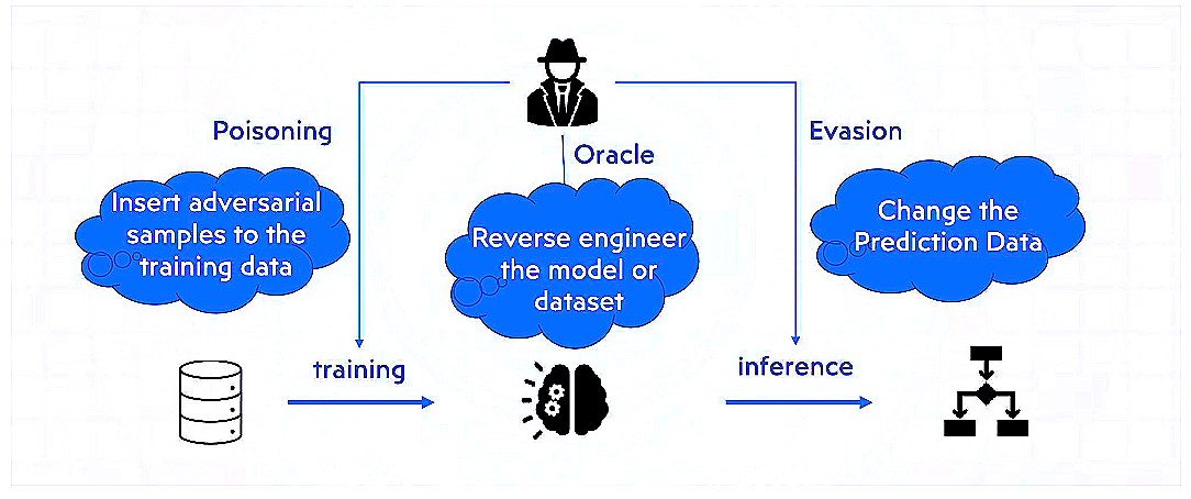
Figure 1: Data Poisoning.

In this study [50],[51],[52],[53],[54], a scenario in which a model owner aims to train a deep learning model based on the training dataset provided by a third party (Figure.1) is considered. However, the third party can poison the training dataset to hijack the model in the future. We assume that the model owner and the trusted third party play the roles of defender and attacker, respectively, in the threat model. The threat model is shown in Figure 2. The knowledge that an attacker can access can generally be classified [55] into two categories. Figure 2: White and black box settings. In a white-box environment, the adversary understands and controls the target dataset and model, including the ability to access and modify the dataset, as well as parameters and the structure of the model. However, in the stricter framework of the black-box, the attacker is only able to manipulate part of the training data but has no knowledge of the structure and parameters of the target model, such as weights, hyperparameters, configurations, etc.

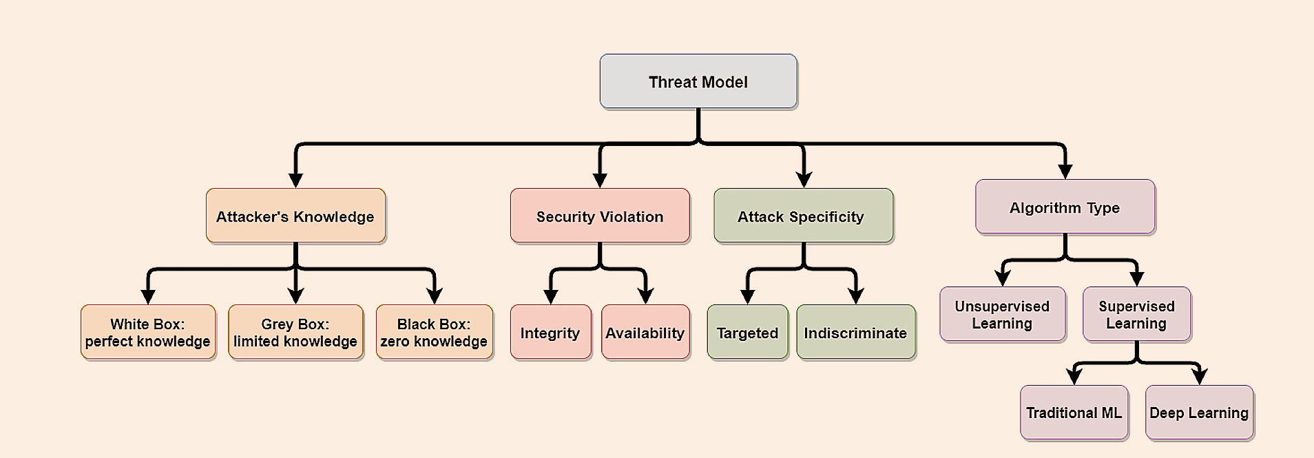
Figure 2: knowledge.

By deliberately misclassifying the inputs with the trigger (Figure 3) as the adversary’s intended labels, the adversary uses a backdoor approach to keep the victim model operating at a high level of accuracy on normal samples. The adversary seeks to have the target model behave as expected on benign data while operating in a way described by the adversary on samples that have been poisoned, as seen in Figure 2. A formulation of the enemy’s objective is:

$$\min_{\mathcal{M}^{*}}\mathcal{L}\left(\mathcal{D}^{b},\mathcal{D}^{p},\mathcal{M}^{*}\right)= \sum_{x_{i}\in\mathcal{D}^{b}}l\left(\mathcal{M}^{*}\left(x_{i}\right),y_{i}\right)$$

$$+\sum_{x_{j}\in\mathcal{D}^{p}}l\left(\mathcal{M}^{*}\left(x_{r}\circ\varepsilon\right),y_{t}\right),$$

where $\mathcal{D}^{b}$ and $\mathcal{D}^{p}$ represent the benign and poisoned training datasets, respectively. The function $l(\cdot,\cdot)$ denotes the loss function which depends on the specific task. The symbol $\circ$ denotes the operation of integrating the backdoor trigger $(\varepsilon)$ into the training data.

III Adversarial Machine Learning in Finance via Bayesian Approach

Data: T, $\theta$, $\alpha$, $\beta$, $\sigma$

Result: Model parameters and trace.

Initialize $x_{T}$;

for $t\leftarrow T-1$ downto $0$ do

       if $t>1$ then

             $z\leftarrow$ Noise_dist$(0)$;

            

      Else $z\leftarrow 0$;

       $transport\_component\leftarrow$ Optimal_transport$(x_{T},t,\theta,\beta,\sigma)$;

       $x_{t-1}\leftarrow$ Normal$(f^{\prime}x_{t}^{\prime},\mu=drift\_function(x_{T},t,\theta,\beta,\sigma)+transport\_component+\sigma[t]\cdot z,\sigma=1)$;

       $x_{T}\leftarrow x_{t-1}$;

      

Algorithm 1 Diffusion Bayesian Optimization

Data: $\theta$, $\alpha$, $\beta$, $\sigma$

Result: Priors for $\theta$, $\alpha$, $\beta$, $\sigma$

Define hierarchical priors for each parameter group;

for each parameter group do

       if parameter group is $\theta$ then

             $\theta\sim\mathcal{N}(0,1)$;

            

       end if

      else if parameter group is $\alpha$ then

             $\alpha\sim\mathcal{N}(0,1)$;

            

       end if

      else if parameter group is $\beta$ then

             $\beta\sim\mathcal{N}(0,1)$;

            

       end if

      else if parameter group is $\sigma$ then

             $\sigma\sim\mathcal{N}(0,1)$;

            

       end if

      

end for

Algorithm 2 Setting up hierarchical priors

Data: T, S0, $\sigma$, $\gamma$, dt

Result: paths

$N\leftarrow len(S0)$

$paths[0]\leftarrow S0$

for $t=1$ to Tdt do

       $dW\leftarrow\mathcal{N}(0,1;size=N)$

       $dX\leftarrow dt(\gamma\cdot paths[t-1]+\sigma\cdot dW)$

       $paths[t]\leftarrow paths[t-1]+dX$

      

end for

return $paths$

Algorithm 3 Simulate Rough Volatility Paths

Either a portfolio $\phi_{t}$ a $K+1$-dimensional vector $\phi_{t}\in\mathbb{R}^{K+1}$. Where a portfolio $\phi_{t}=\left(\phi_{t}^{0},\ldots,\phi_{t}^{K}\right)$ gives the number $\phi_{t}^{k}$ of every security $k\in\{0,\ldots,K\}$ held by an agent at date $t$. This portfolio is then labeled $\phi_{1}$, and has to be held during the time interval $[0,1[$. $\phi_{t}^{0}$ represents the number of bonds in the portfolio $\phi_{t}$ at date $t$

The market value $V_{t}$ of a portfolio $\phi_{t}$ in $S$ at date $t$ is given by a function $V_{t}:\mathbb{R}^{K+1}\times\mathbb{R}_{++}^{K+1}\rightarrow\mathbb{R}$ where,

$$V_{t}(\phi,S)\equiv\begin{cases}\phi_{1}\cdot S_{0}&\text{ for }t=0\\ \phi_{t}\cdot S_{t}&\text{ for }t\in\{1,\ldots,T\}\end{cases}$$

Input: Initial stock price $S$, strike price $K$, time to maturity $T$, risk-free interest rate $r$, volatility $\sigma$

Output: Call option price

$d_{1}=\frac{\ln\left(\frac{S}{K}\right)+\left(r+\frac{1}{2}\sigma^{2}\right)T}{\sigma\sqrt{T}}$

$d_{2}=d_{1}-\sigma\sqrt{T}$

$call\_price=S\cdot N(d_{1})-K\cdot e^{-rT}\cdot N(d_{2})$

return $call\_price$

Algorithm 4 Calculate Call Option Price

Data: $x_{T}$, $t$, $\theta$, $\mu$, $\sigma$

Result: Deterministic movement.

$movement=\theta\cdot(\mu-x_{T})+\sigma\cdot\sqrt{\frac{1}{\theta}\left(1-e^{-\theta\cdot t}\right)}\cdot\mathcal{N}(0,\,1)$;

return $movement$;

Algorithm 5 Optimal Transport

Input: Initial portfolio value, Stock price $S$, strike price $K$, time to maturity $T$, risk-free interest rate $r$, volatility $\sigma$, time step $dt$

Output: Final portfolio value after hedging.

Initialize $\delta,\gamma,\theta$ using calculate_greeks($S$, $K$, $T$, $r$, $\sigma$)

for $t=0$ to $T/dt$ do

       Simulate $S_{new}=S+N(0,\sigma dt)S$

       Recalculate $\delta_{new},\theta_{new}$ using calculate_greeks($S_{new}$, $K$, $T$, $r$, $\sigma$)

       Adjust portfolio: $portfolio\_adjustment=\delta_{new}(S_{new}-S)+\gamma(S_{new}-S)^{2}$

       Update $S=S_{new}$ and initial_portfolio_value += $portfolio\_adjustment$

      

end for

return initial_portfolio_value

Algorithm 6 Dynamic Hedging

Input: Stock price $S$, strike price $K$, time to maturity $T$, risk-free interest rate $r$, volatility $\sigma$

Output: Delta, Gamma, Theta

$call\_price=\texttt{black\_scholes\_merton\_call}(S,K,T,r,\sigma)$

$d_{1}=\frac{\ln\left(\frac{S}{K}\right)+\left(r+\frac{1}{2}\sigma^{2}\right)T}{\sigma\sqrt{T}}$

$d_{2}=d_{1}-\sigma\sqrt{T}$

$\delta=N(d_{1})$

$\gamma=N^{\prime}(d_{1})\frac{S\sigma\sqrt{T}}{1}$

$\theta=-0.5\sigma^{2}STN^{\prime}(d_{1})-rK\cdot e^{-rT}N(d_{2})$

$Vega=S\cdot\sqrt{T}\cdot\text{norm.pdf}(d_{1})$

$\rho=K\cdot e^{-rT}\cdot\text{norm.cdf}(d_{2})$

return $\delta,\gamma,\theta$

Algorithm 7 Calculate Greeks

Input: Objective function $f(x)$, Bounds $B$

Output: Optimized parameters $x^{*}$, Best value $v^{*}$

Initialize Bayesian optimizer with $f$ and $B$

while Stopping criterion not met do

       Sample $x$ from the prior distribution

       Evaluate $f(x)$

       Update the posterior distribution based on $f(x)$

       Select next query point $x^{\prime}$ based on acquisition function

       Evaluate $f(x^{\prime})$

       Update the best known value $v^{*}$ and corresponding parameters $x^{*}$

      

end while

Return $x^{*}$ and $v^{*}$

Algorithm 8 Bayesian Optimization Process

III-A Bayesian optimization formalization.

Formally, the purpose of BO (Bayesian-Optimization) [56],[57] is to retrieve the optimum $\mathbf{x}^{\star}$ of a black-box function $f(\mathbf{x})$ where $\mathbf{x}\in\mathcal{X}$ and $\mathcal{X}$ is the input space where $f(\mathbf{x})$ can be observed. We want to retrieve $\mathbf{x}^{\star}$ such that,

$$\mathbf{x}^{\star}=\arg\min_{\mathbf{x}\in\mathcal{X}}f(\mathbf{x}),$$

assuming minimization (or maximization): We can define a BO method by,

$$\mathcal{A}=(\mathcal{M},\alpha(\cdot),p(f(\mathbf{x})\mid\mathcal{D})),$$

where $f(\mathbf{x})$ is the black-box that we want to optimize, $\mathcal{M}$ is a probabilistic surrogate model, $\alpha(\cdot)$ is an acquisition, or decision, function, and $p(f(\mathbf{x})\mid\mathcal{D})$ is a predictive distribution of the observation of $\mathbf{x}$ and $\mathcal{D}=\left\{\left(\mathbf{x}_{i},y_{i}\right)\mid i=1,\ldots,t\right\}$ is the dataset of previous observations at iteration $t$.

IV MarketBackFinal 2.0: Attack Scenario.

“MarketBackFinal 2.0” is a technique that implements a poisoning attack with a ”clean-label backdoor“ [58],[59],[60],[61],[62],[63]. Contains methods such as ‘stochastic investments models‘, rough volatility algorithm 3, optimal transport algorithm 5 (calculating the deterministic movement (transport component) based on the state and time), and dynamic hedging algorithm 6(which takes as calculate Call Option Price algorithm4 and calculate Greeks algorithm 7), Bayesian Optimization Process algorithm 8, Diffusion Bayesian Optimization algorithm 1 (which takes as setting up hierarchical priors algorithm 2 ) to apply the attack to the audio data, Bayesian style is implemented using a “prior” (Bayesian optimization over the given objective function) and the BO framework with drifts functions including Diffusion Bayesian Optimization. Thanks to this technique, process volatility effects in the drift function (incorporating the transport component into the drift functions) are used for sampling to obtain and define the prior distribution, and a diffusion technique is then applied, which implements a diffusion-based sampling technique to generate a sequence of samples as a function of certain parameters and a noise distribution. The Bayesian method integrates the drift function into the Bayesian model in the “MarketBackFinal 2.0” method while using a NUTS method for sampling (efficient sampling with adaptive step size Hamiltonian Monte Carlo). Given a time step $T$ and a set of parameters $\alpha,\beta,\sigma,\theta$, the method generates a new data point $x_{T}$ based on the current state $x_{T-1}$ and the noise distribution $sin(x)$. The results are available on ART.1.18; link: https://github.com/Trusted-AI/adversarial-robustness-toolbox/pull/2467.

V Experimental results

V-A Datasets Descritpion.

We use the ESC-50 environmental dataset [64], the dataset ESC-50 (environmental), is a labeled collection of 2,000 environmental sounds, which comprises five-second recordings sorted into 50 semantic categories (with 40 examples per category) that are further divided into five main groups: animals; natural soundscapes and water sounds; humans, non-vocal sounds; indoor/domestic sounds; and outdoor/urban sounds. The audio tracks from the various datasets were pre-processed using the librosa package in Python, which extracts spectrogram features from the audio tracks. For our methods, we used the extracted features and spectrogram images.

V-B Victim models.

Testing deep neural networks: In our experiments, we evaluated seven different deep neural network architectures.) proposed in the literature for speech recognition. In particular, we used a Whisper (OpenAI) described in [65], an facebook/w2v-bert-2.0 (Facebook) described in [66], facebook/mms-1b-all described in [67], an wav2vec 2.0 described in [68], an Data2vec described in [69], an HuBERT described in [70] and a Speech Encoder Decoder Models described in [71]. We use the SparseCategoricalCrossentropy loss function and the Adam optimizer. The learning rates for all models are set to 0.1. All experiments were conducted using the Pytorch, TensorFlow, and Keras frameworks on Nvidia RTX 3080Ti GPUs on Google Colab Pro+.

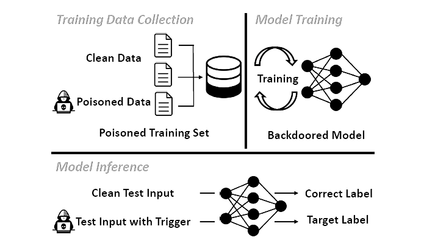
Figure 3: Illustrates the execution process of a backdoor attack.

V-C Evaluation Metrics.

To measure the performance of backdoor attacks Figure 3, two common metrics are used [72] [73]: benign accuracy (BA) and attack success rate (ASR). BA measures the classifier’s accuracy on clean (benign) test examples. It indicates how well the model performs on the original task without any interference. ASR, in turn, measures the success of the backdoor attack, i.e., in causing the model to misclassify poisoned test examples. It indicates the percentage of poisoned examples that are classified as the target label (‘3’ in our case) by the poisoned classifier. Formally, it can be expressed as:

$$ASR=\frac{\sum_{i=1}^{N}\mathbb{I}\left(\mathcal{M}^{*}\left(x_{i}\circ\varepsilon\right)=y_{t}\right)}{N},$$

where $\mathbb{I}(\cdot)$ is the indicator function, $\mathcal{M}^{*}$ is the target model, and $x_{i}\circ\varepsilon$ and $y_{t}$ denote the poisoned sample and target label, respectively.

$$BA=\frac{\sum_{i=1}^{M}\mathbb{I}\left(\mathcal{M}^{*}\left(x_{i}\right)=y_{i}\right)}{M}$$

Table I: Performance comparison of backdoored models.

Hugging Face Models	Benign Accuracy (BA)	Attack Success Rate (ASR)
wav2vec 2.0	94.73%	100%
whisper (OpenAI)	95.03%	100%
HuBERT	95.21%	100%
facebook/w2v-bert-2.0(Facebook)	98.96%	100%
facebook/mms-1b-all	93.31%	100%
Speech Encoder Decoder	96.12%	100%
Data2vec	99.12%	100%

• ESC-50 environmental dataset.

Table I presents the different results obtained using our backdoor attack approach (MarketBackFinal 2.0) on pre-trained models (transformers available on Hugging Face). We can see that our backdoor attack easily manages to mislead these models (readers are invited to test), other Hugging Face models; as far as we know, we’ve managed to fool almost all these models.

V-D Characterizing the effectiveness of MarketBackFinal 2.0.

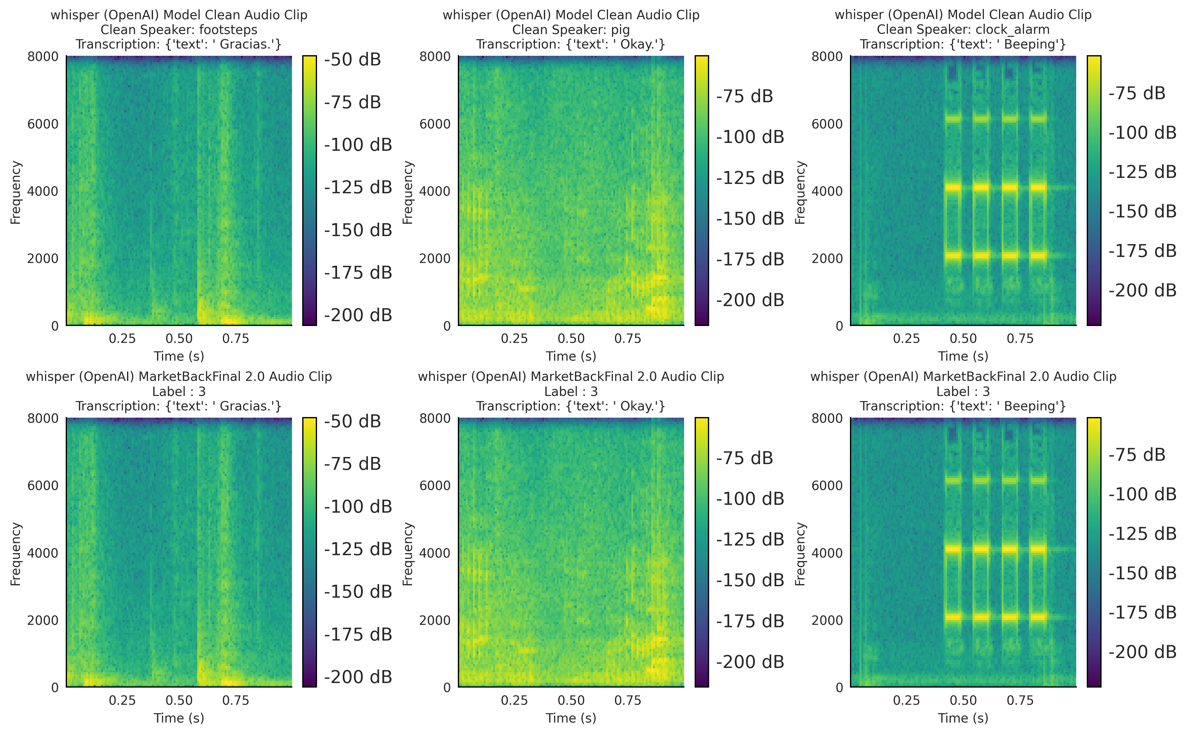
Figure 4: The top graphs show three distinct clean spectrograms (for each genre with its unique ID (sound)), and the bottom graphs show their respective (backdoored) equivalents (by MarketBackFinal 2.0) (which predict the label set by the attacker, i.e., 3), with decisions taken by the whisper (OpenAI) model (table I).

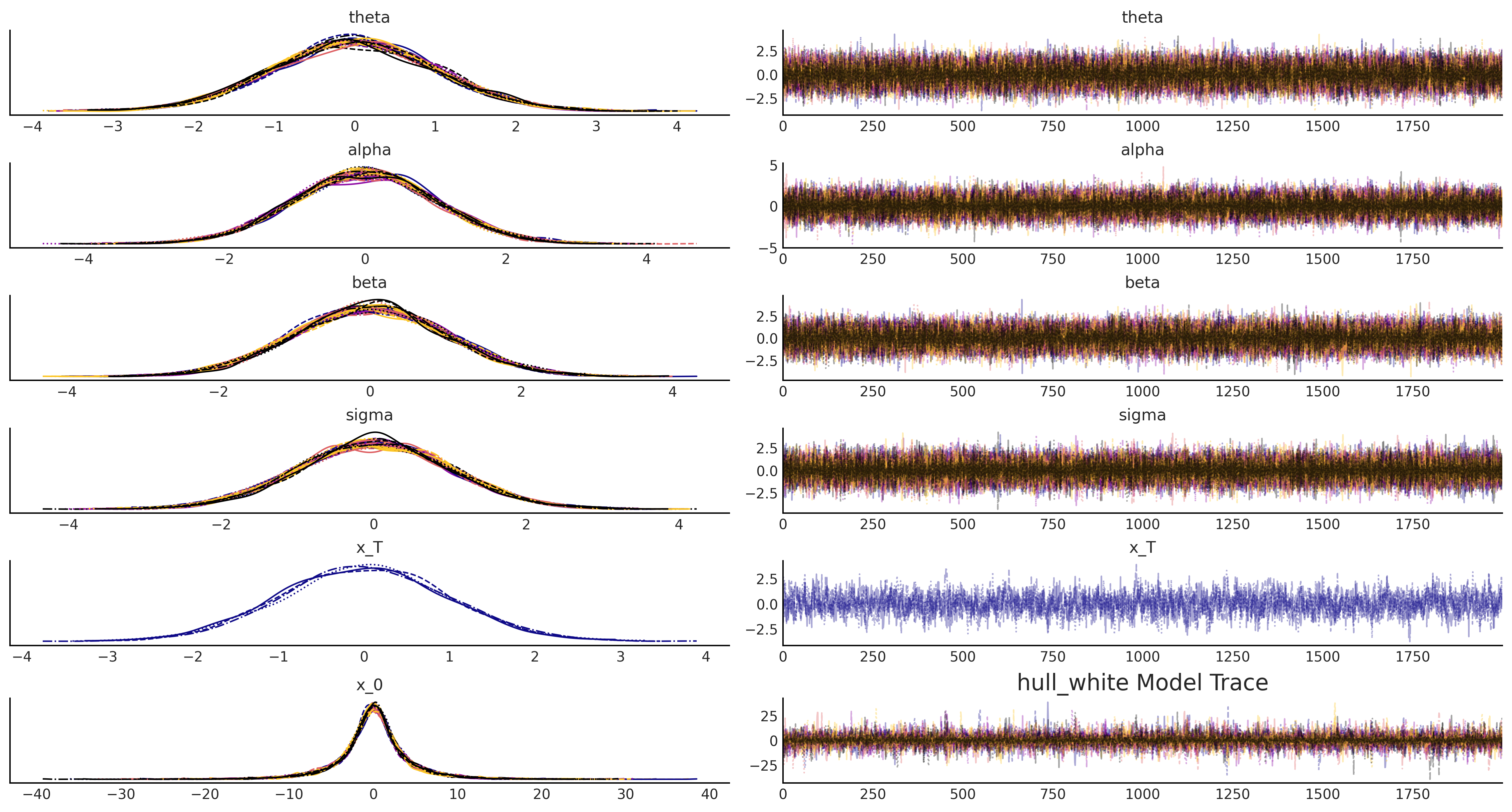
Figure 5: Dataset ESC 50: Backdoor attack (MarketBackFinal 2.0) Hull White model bayesian optimization. Table I).

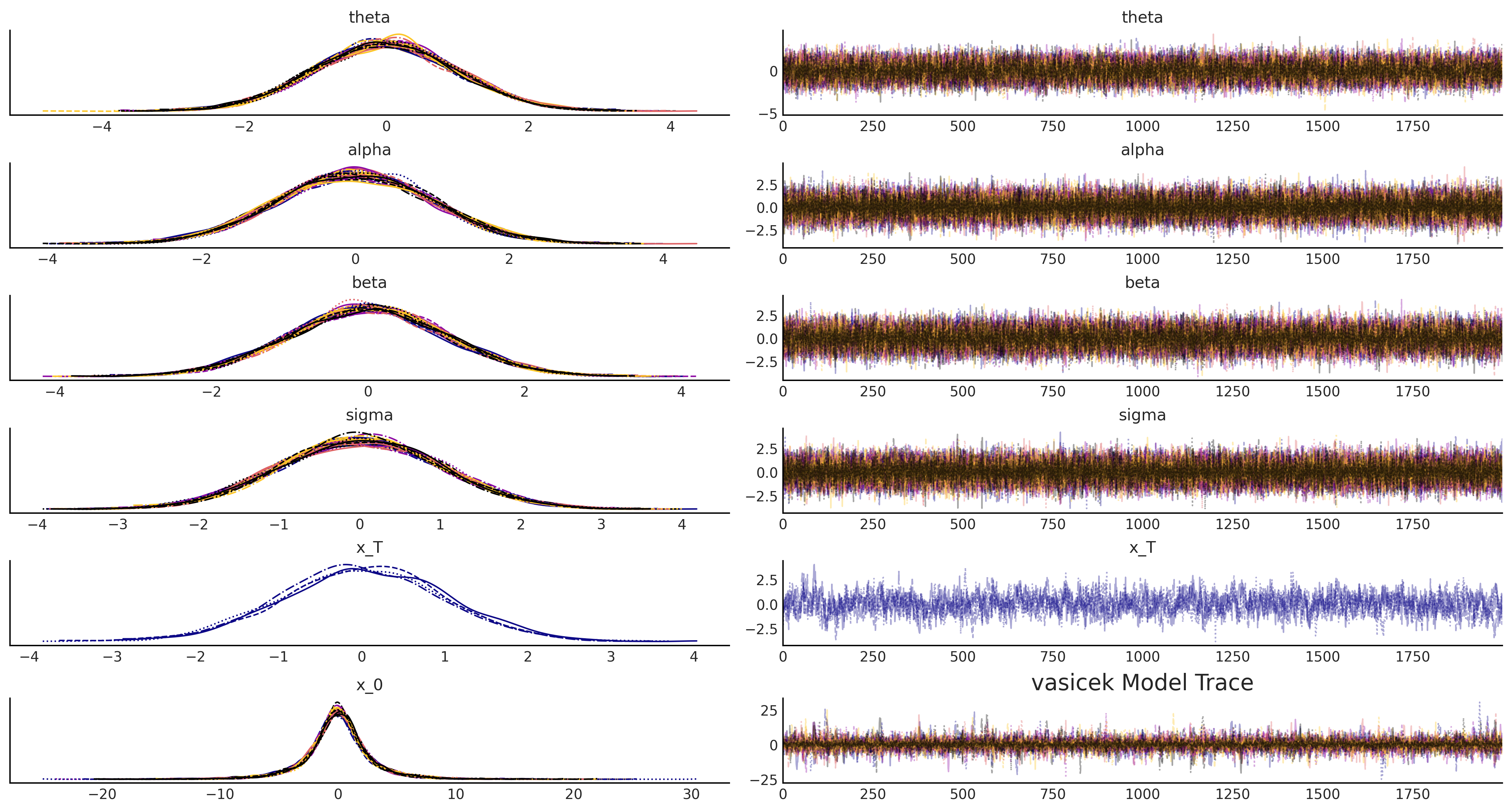
Figure 6: ESC-50: Backdoor attack (MarketBackFinal 2.0) Vasieck model bayesian optimization. Table I).

Figure 7: ESC-50: Backdoor attack (MarketBackFinal 2.0) Longstaff-Schwartz model bayesian optimization. Table I).

Figure 8: ESC-50: Backdoor attack (MarketBackFinal 2.0) Libor market model bayesian optimization. Table I).

V-E Bayesian dynamic hedging via stochastic investment models .

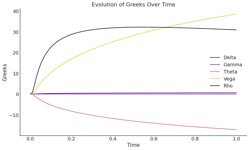
Figure 9: ESC-50: Backdoor attack (MarketBackFinal 2.0) dynamic hedging by bayesian optimization. Table I).

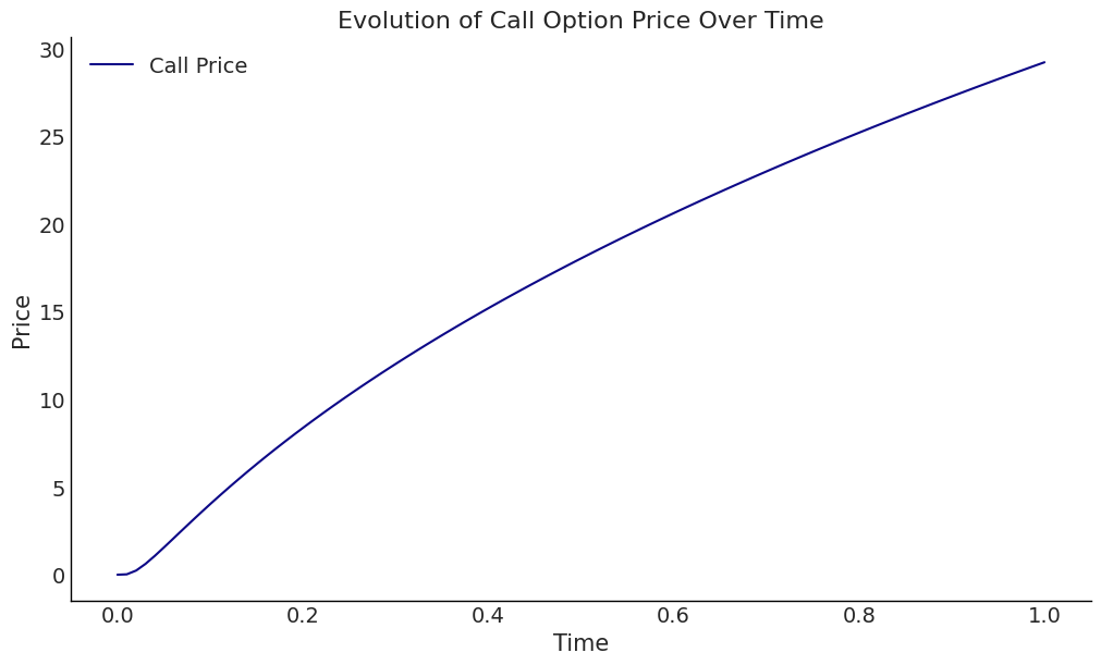
Figure 10: ESC-50: Backdoor attack (MarketBackFinal 2.0) Call Option Price by bayesian optimization. Table I).

V-F Financial Modeling Using Various Inversion Models via Diffusion Drift Optimized by Bayesian Simulation.

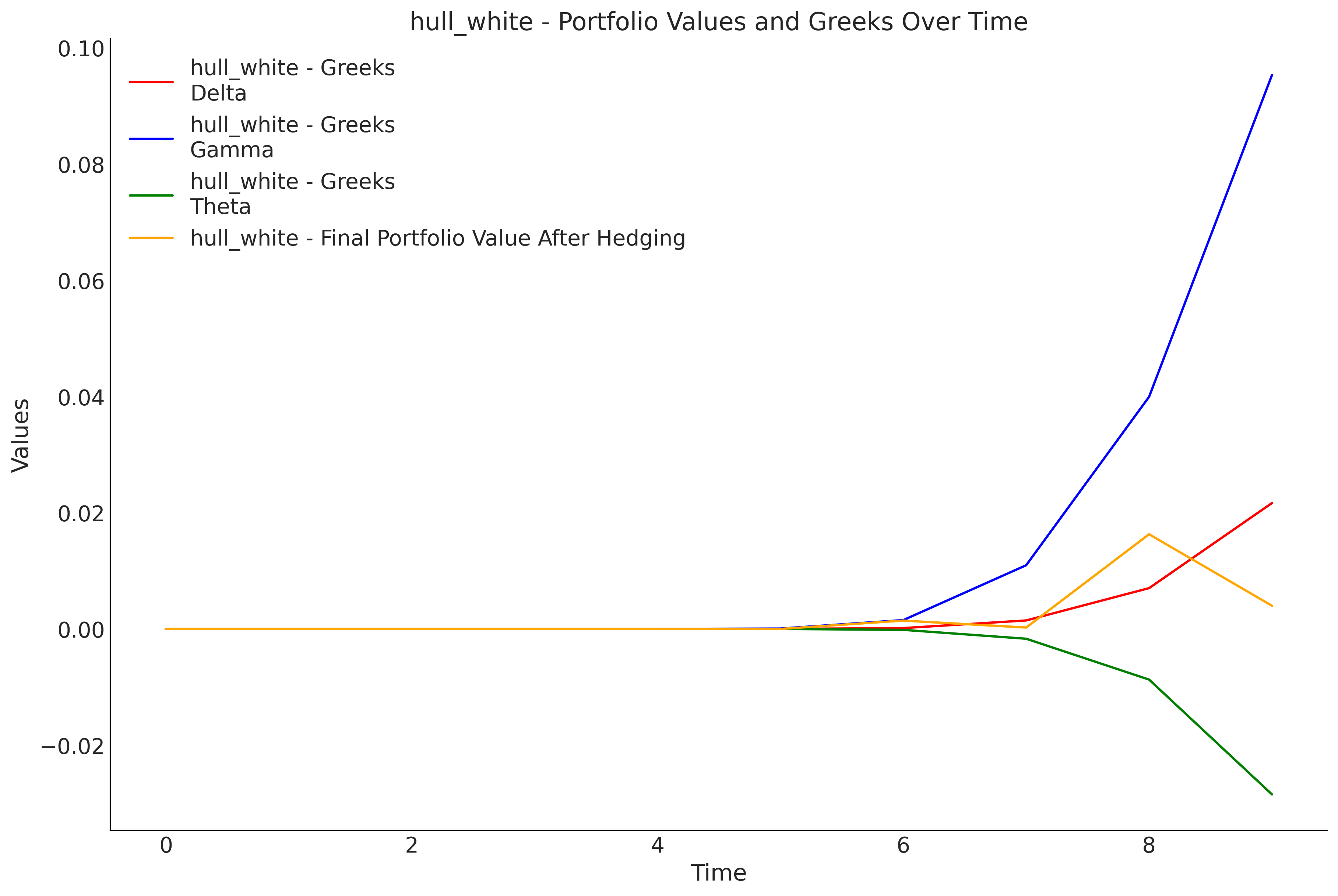
Figure 11: Dynamic Hedging: Hull White model.

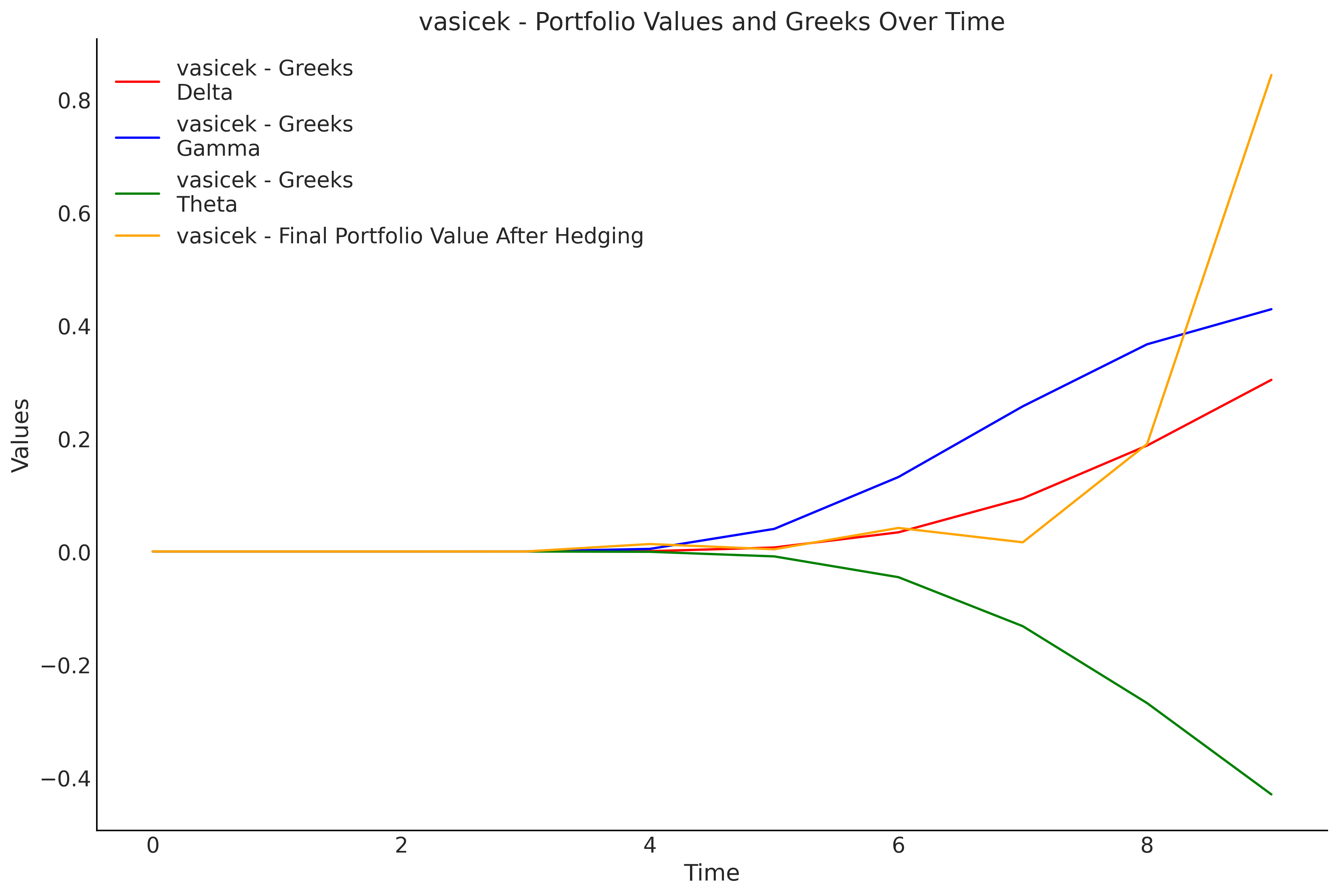
Figure 12: Dynamic Hedging: Vasieck model.

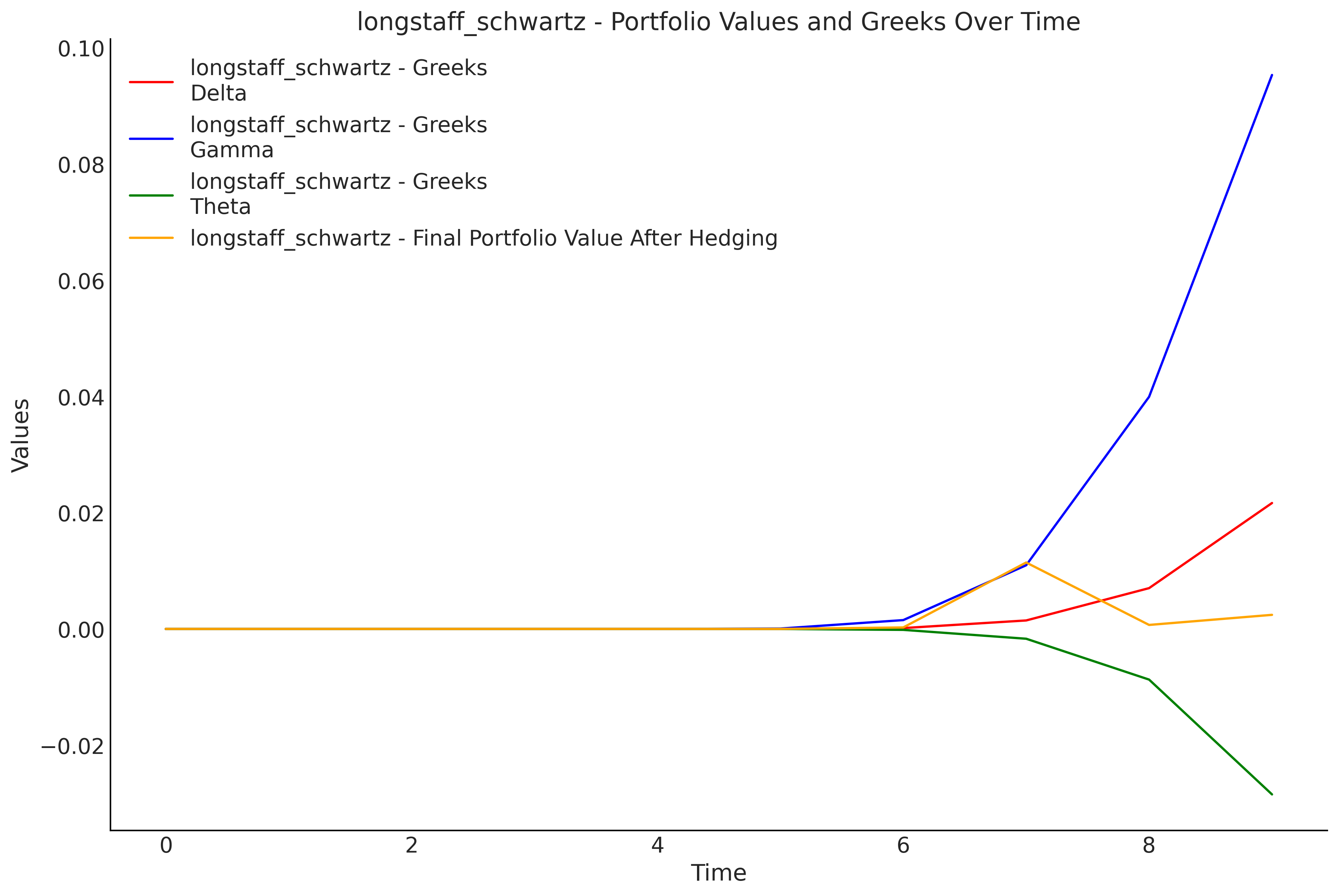
Figure 13: Dynamic Hedging: Longstaff-Schwartz model.

Figure 14: Dynamic Hedging : Libor market model.

Conclusions

The weaknesses of transformer-based generative artificial intelligence models are the main subject of this work, which also showcases a new financial simulation tool. A clean-label backdoor and poisoning attack specifically designed for financial modeling using various inversion models via diffusion drift optimized by Bayesian[74] simulation is known as “MarketBackFinal 2.0,” and it is one of the attack methods developed in this article. Function simulations utilize hierarchical hypothesis parameters. With the primary goal of using them with financial data, this article concentrates on the development of new financial simulation tools. But in order to ensure that the approach method operates as intended, temporal acoustic data obtained through a backdoor assault is used for validation. Audio backdoor attacks based on Bayesian transformations (using a drift function via stochastic investment model effects for sampling [75]) based on a diffusion model approach (which adds noise). The study results help to understand the potential but also the risks and vulnerabilities to which pre-trained advanced DNN models are exposed via malicious audio manipulation to ensure the security and reliability of automatic speech recognition audio models.

Financial understanding of the concepts of Stock market

Concepts of LIBOR Market.

Definition .1 (LIBOR Market).

The $\delta_{i}$-forward-LIBOR rate $L_{i}(t)$ is the simple yield for the time interval $\left[t_{i-1},t_{i}\right]$, i.e. with $\delta_{i}=t_{i}-t_{i-1}$ we define:

$$L_{i}(t)=L\left(t;t_{i-1},t_{i}\right)=\frac{1}{\delta_{i}}\frac{P\left(t,t_{i-1}\right)-P\left(t,t_{i}\right)}{P\left(t,t_{i}\right)}.$$

By the definition of the $t_{i}$-forward measure $\mathbb{Q}_{i}:=\mathbb{Q}_{t_{i}}$, $L_{i}(t)$ is a $\mathbb{Q}_{i}$-martingale. Thus, it is an immediate consequence that if we want to model log-normal forward-LIBOR rates in a diffusion setting, we have to choose the following dynamics under $\mathbb{Q}_{i}$ :

$$dL_{i}(t)=L_{i}(t)\sigma_{i}(t)dW_{i}(t),$$

Here, $W_{i}($.$)$ is a (for the moment one-dimensional) $\mathbb{Q}_{i}$-Brownian motion, $\sigma_{i}(t)$ a bounded and deterministic function.

Remark.

The risk-free deposit rates $D_{s}^{i}$ for deposits between $t_{i}$ and $t_{i+1}$ are defined by,

$$1+\delta_{i}D_{s}^{i}=\frac{P^{D}\left(s,t_{i}\right)}{P^{D}\left(s,t_{i+1}\right)}.$$

The factors $\delta_{i}$ are the accrual factors or day count fractions and represent the fraction of the year spanned by the interval $\left[t_{i},t_{i+1}\right]$ .

$$dD_{t}^{j}=\gamma_{j}\left(D_{t}^{j},t\right)\cdot dW_{t}^{j+1}$$

$\gamma_{j}(0\leq j\leq n-1)$ are $m$-dimensional functions. The Brownian motion change between the $N_{t}$ and the $P^{D}\left(t,t_{j+1}\right)$ is given by,

$$dW_{t}^{j+1}=dW_{t}+\nu\left(t,t_{j+1}\right)dt.$$

$\nu\left(t,t_{j+1}\right)-\nu\left(t,t_{j}\right)$ can be written [76] as:

$$\nu\left(t,t_{j+1}\right)-\nu\left(t,t_{j}\right)=\frac{1}{D_{t}^{j}+\frac{1}{\delta_{j}}}\gamma_{j}\left(D_{t}^{j},t\right)$$

$$dW_{t}^{j+1}=-\sum_{i=j+1}^{n-1}\frac{1}{D_{t}^{i}+\frac{1}{\delta_{i}}}\gamma_{i}\left(D_{t}^{i},t\right)dt+dW_{t}^{n}.$$

$$dL_{t}^{j}=-\left(\sum_{i=j+1}^{n-1}\frac{1}{D_{t}^{i}+\frac{1}{\delta_{i}}}\gamma_{i}\left(D_{t}^{i},t\right)\cdot\gamma_{j}\left(D_{t}^{j},t\right)\right)dt+$$

$$\gamma_{j}\left(D_{t}^{j},t\right)\cdot dW_{t}^{n}.$$

by incorporating a diffusion approximation with $a_{i}\leq 1/\delta_{i}$ we have,

$$\gamma_{j}(D,t)=\alpha(t)\left(D+a_{j}\right)\gamma_{j}$$

$$dD_{t}^{j}=-\alpha^{2}(t)\left(\sum_{i=j+1}^{n-1}\frac{D_{t}^{i}+a_{i}}{D_{t}^{i}+\frac{1}{\delta_{i}}}\gamma_{i}\cdot\gamma_{j}\right)\left(D_{t}^{j}+a_{j}\right)dt+$$

$$\alpha(t)\left(D_{t}^{j}+a_{j}\right)\gamma_{j}\cdot dW_{t}^{n}.$$

with $\alpha$ a deterministic scalar function, $a$ a constant vector of dimension $n$ and $\left(\gamma_{j}\right)_{j=1,\ldots,n}$ vectors of dimension $m$.

Theorem 1.

Cap pricing and the Black formula, for $i=1,\ldots,N$ the $\delta_{i}$ forward-LIBOR rates satisfy,

$$dL_{i}(t)=L_{i}(t)\sigma_{i}(t)dW_{i}(t),t<t_{i}.$$

(a) Then today’s price $C_{i}\left(t,\sigma_{i}(t)\right)$ of a caplet maturing at time $t_{i}$ with a payment of $\delta_{i}\cdot\left(L_{i}\left(t_{i}\right)-L\right)^{+}$is given by,

$$\begin{gathered}C_{i}\left(t,\sigma_{i}(t)\right)=\delta_{i}P\left(t,t_{i}\right)\left[L_{i}(t)\Phi\left(d_{1}(t)\right)-L\Phi\left(d_{2}(t)\right)\right],\\ d_{1}(t)=\frac{\ln\left(\frac{L_{i}(t)}{L}\right)+\frac{1}{2}\bar{\sigma}_{i}^{2}(t)}{\bar{\sigma}_{i}(t)},d_{2}(t)=d_{1}(t)-\bar{\sigma}_{i}(t),\\ \bar{\sigma}_{i}^{2}(t)=\int_{t}^{t_{i-1}}\sigma^{2}(s)ds.\end{gathered}$$

(b) Today’s price of a cap in the forward-LIBOR model $\operatorname{Cap}_{FL}(t;V,L)$ with payment times $t_{1}<\ldots<t_{N}$ and level $L$ is given by,

$$\operatorname{Cap}_{FL}(t;V,L)=V\cdot\sum_{i=1}^{N}C_{i}\left(t,\sigma_{i}(t)\right).$$

In particular, if all volatility processes satisfy $\sigma_{i}(t)=\sigma$ for some positive constant $\sigma$ then we have

$$\operatorname{Cap}_{FL}(t;V,L)=\operatorname{Cap}_{\text{Black }}(t,V,L,\sigma),$$

i.e. the price of the cap equals the one obtained with the Black formula.

Concepts of hedging.

For hedging and risk management, the delta [77],[78] $\Delta=\frac{\partial V}{\partial S}$, i.e. the first partial derivative of the option’s value with respect to the index level: For the Greeks of a European call option.

$$\Delta=\frac{\partial C}{\partial S}=N\left(d_{1}\right)$$

The gamma is the second partial derivative with respect to the index level,

$$\gamma=\frac{\partial^{2}C}{\partial S^{2}}=\frac{N^{\prime}\left(d_{1}\right)}{S\sigma\sqrt{T-t}}$$

The theta of an option is, by convention, the negative first partial derivative with respect to time-to-maturity $t^{*}=T-t$

$$\theta=-\frac{\partial C}{\partial t^{*}}=-\frac{SN^{\prime}\left(d_{1}\right)\sigma}{2\sqrt{T-t}}-re^{-r(T-t)}KN\left(d_{2}\right)$$

The rho of an option is the first partial derivative with respect to the short rate $r$

$$\rho=\frac{\partial C}{\partial r}=K(T-t)e^{-r(T-t)}N\left(d_{2}\right)$$

The vega-which is obviously not a Greek letter-is the first partial derivative with respect to the volatility $\sigma$,

$$\mathbf{vega}=\frac{\partial C}{\partial\sigma}=SN^{\prime}\left(d_{1}\right)\sqrt{T-t}$$

Hedging dynamics can be defined as:

$$\Delta_{t}^{P}\equiv\frac{\partial P_{t}}{\partial S_{t}}$$

$$dP_{t}-\Delta_{t}^{P}dS_{t}=0$$

Investment banks are also often interested in replicating the payoff of such a put (or another option). This is accomplished by setting up a replication portfolio consisting of $\Delta_{t}^{P}$ units of the underlying and $\gamma_{t}\equiv P_{t}-\Delta_{t}^{P}S_{t}$ units of the risk-less bond $B_{t}$ such that the resulting portfolio value equals the option value at any time $t$,

$$P_{t}=\Delta_{t}^{P}S_{t}+\gamma_{t}B_{t}$$

or

$$dP_{t}=\Delta_{t}^{P}dS_{t}+\gamma_{t}dB_{t}$$

For a plain vanilla put option this generally implies being short the underlying $\left(\Delta_{t}^{P}<0\right)$ and long the bond. For a call option $\left(\Delta_{t}^{C}>0\right)$ this implies the opposite. A replication strategy $\left(\Delta_{t}^{P},\gamma_{t}\right),t\in\{0,\ldots,\tau-\Delta t\}$, is called self-financing if for $t>0$ and $\tau$ being the exercise date (i.e. $\tau=T$ for a European option)

$$\Delta_{t}^{P}S_{t}+\gamma_{t}B_{t}=\Delta_{t-\Delta t}^{P}S_{t}+\gamma_{t-\Delta t}B_{t}.$$

References

- [1] G. Yenduri, M. Ramalingam, G. C. Selvi, Y. Supriya, G. Srivastava, P. K. R. Maddikunta, G. D. Raj, R. H. Jhaveri, B. Prabadevi, W. Wang et al., “Gpt (generative pre-trained transformer)–a comprehensive review on enabling technologies, potential applications, emerging challenges, and future directions,” IEEE Access, 2024.
- [2] M. Gupta, C. Akiri, K. Aryal, E. Parker, and L. Praharaj, “From chatgpt to threatgpt: Impact of generative ai in cybersecurity and privacy,” IEEE Access, 2023.
- [3] A. Troxler and J. Schelldorfer, “Actuarial applications of natural language processing using transformers: Case studies for using text features in an actuarial context,” British Actuarial Journal, vol. 29, p. e4, 2024.
- [4] Y. Yao, J. Duan, K. Xu, Y. Cai, Z. Sun, and Y. Zhang, “A survey on large language model (llm) security and privacy: The good, the bad, and the ugly,” High-Confidence Computing, p. 100211, 2024.
- [5] Z. Wang and Q. Hu, “Blockchain-based federated learning: A comprehensive survey,” arXiv preprint arXiv:2110.02182, 2021.
- [6] L. Sun, Y. Huang, H. Wang, S. Wu, Q. Zhang, C. Gao, Y. Huang, W. Lyu, Y. Zhang, X. Li et al., “Trustllm: Trustworthiness in large language models,” arXiv preprint arXiv:2401.05561, 2024.
- [7] L. Cao, “Ai in finance: challenges, techniques, and opportunities,” ACM Computing Surveys (CSUR), vol. 55, no. 3, pp. 1–38, 2022.
- [8] C.-J. Wu, R. Raghavendra, U. Gupta, B. Acun, N. Ardalani, K. Maeng, G. Chang, F. Aga, J. Huang, C. Bai et al., “Sustainable ai: Environmental implications, challenges and opportunities,” Proceedings of Machine Learning and Systems, vol. 4, pp. 795–813, 2022.
- [9] M. Zawish, F. A. Dharejo, S. A. Khowaja, S. Raza, S. Davy, K. Dev, and P. Bellavista, “Ai and 6g into the metaverse: Fundamentals, challenges and future research trends,” IEEE Open Journal of the Communications Society, vol. 5, pp. 730–778, 2024.
- [10] R. Bommasani, D. A. Hudson, E. Adeli, R. Altman, S. Arora, S. von Arx, M. S. Bernstein, J. Bohg, A. Bosselut, E. Brunskill et al., “On the opportunities and risks of foundation models,” arXiv preprint arXiv:2108.07258, 2021.
- [11] J. Z. Pan, S. Razniewski, J.-C. Kalo, S. Singhania, J. Chen, S. Dietze, H. Jabeen, J. Omeliyanenko, W. Zhang, M. Lissandrini et al., “Large language models and knowledge graphs: Opportunities and challenges,” arXiv preprint arXiv:2308.06374, 2023.
- [12] O. Mengara, “The art of deception: Robust backdoor attack using dynamic stacking of triggers,” arXiv preprint arXiv:2401.01537, 2024.
- [13] Y. Li, S. Wang, H. Ding, and H. Chen, “Large language models in finance: A survey,” in Proceedings of the fourth ACM international conference on AI in finance, 2023, pp. 374–382.
- [14] K. Peng and G. Yan, “A survey on deep learning for financial risk prediction,” Quantitative Finance and Economics, vol. 5, no. 4, pp. 716–737, 2021.
- [15] J. Lee, N. Stevens, S. C. Han, and M. Song, “A survey of large language models in finance (finllms),” arXiv preprint arXiv:2402.02315, 2024.
- [16] Y. Nie, Y. Kong, X. Dong, J. M. Mulvey, H. V. Poor, Q. Wen, and S. Zohren, “A survey of large language models for financial applications: Progress, prospects and challenges,” arXiv preprint arXiv:2406.11903, 2024.
- [17] X. Huang, W. Ruan, W. Huang, G. Jin, Y. Dong, C. Wu, S. Bensalem, R. Mu, Y. Qi, X. Zhao et al., “A survey of safety and trustworthiness of large language models through the lens of verification and validation,” Artificial Intelligence Review, vol. 57, no. 7, p. 175, 2024.
- [18] O. Mengara, “The last dance: Robust backdoor attack via diffusion models and bayesian approach,” arXiv preprint arXiv:2402.05967, 2024.
- [19] ——, “Trading devil: Robust backdoor attack via stochastic investment models and bayesian approach,” arXiv. org, Tech. Rep., 2024.
- [20] M. Joshi and A. Stacey, “New and robust drift approximations for the libor market model,” Quantitative Finance, vol. 8, no. 4, pp. 427–434, 2008.
- [21] C. Bayer, P. K. Friz, M. Fukasawa, J. Gatheral, A. Jacquier, and M. Rosenbaum, Rough volatility. SIAM, 2023.
- [22] J. Gatheral, T. Jaisson, and M. Rosenbaum, “Volatility is rough,” Quantitative finance, vol. 18, no. 6, pp. 933–949, 2018.
- [23] M. Fukasawa and R. Takano, “A partial rough path space for rough volatility,” Electronic Journal of Probability, vol. 29, pp. 1–28, 2024.
- [24] E. Abi Jaber, “Lifting the heston model,” Quantitative finance, vol. 19, no. 12, pp. 1995–2013, 2019.
- [25] R. Cont and P. Das, “Rough volatility: fact or artefact?” Sankhya B, vol. 86, no. 1, pp. 191–223, 2024.
- [26] J. Matas and J. Pospíšil, “On simulation of rough volterra stochastic volatility models,” arXiv preprint arXiv:2108.01999, 2021.
- [27] E. Abi Jaber and S. X. Li, “Volatility models in practice: Rough, path-dependent or markovian?” Path-Dependent or Markovian, 2024.
- [28] G. Brandi and T. Di Matteo, “Multiscaling and rough volatility: An empirical investigation,” International Review of Financial Analysis, vol. 84, p. 102324, 2022.
- [29] O. E. Euch, M. Fukasawa, J. Gatheral, and M. Rosenbaum, “Short-term at-the-money asymptotics under stochastic volatility models,” SIAM Journal on Financial Mathematics, vol. 10, no. 2, pp. 491–511, 2019.
- [30] E. Abi Jaber and O. El Euch, “Multifactor approximation of rough volatility models,” SIAM journal on financial mathematics, vol. 10, no. 2, pp. 309–349, 2019.
- [31] O. El Euch, M. Fukasawa, and M. Rosenbaum, “The microstructural foundations of leverage effect and rough volatility,” Finance and Stochastics, vol. 22, pp. 241–280, 2018.
- [32] O. El Euch and M. Rosenbaum, “The characteristic function of rough heston models,” Mathematical Finance, vol. 29, no. 1, pp. 3–38, 2019.
- [33] E. Abi Jaber and O. El Euch, “Markovian structure of the volterra heston model,” Statistics & Probability Letters, vol. 149, pp. 63–72, 2019.
- [34] A. Galichon, “The unreasonable effectiveness of optimal transport in economics,” arXiv preprint arXiv:2107.04700, 2021.
- [35] L. C. Torres, L. M. Pereira, and M. H. Amini, “A survey on optimal transport for machine learning: Theory and applications,” arXiv preprint arXiv:2106.01963, 2021.
- [36] B. Horvath, A. Jacquier, A. Muguruza, and A. Søjmark, “Functional central limit theorems for rough volatility,” Finance and Stochastics, pp. 1–47, 2024.
- [37] M. Wiese, L. Bai, B. Wood, and H. Buehler, “Deep hedging: learning to simulate equity option markets,” arXiv preprint arXiv:1911.01700, 2019.
- [38] A. Ilhan, M. Jonsson, and R. Sircar, “Optimal static-dynamic hedges for exotic options under convex risk measures,” Stochastic Processes and their Applications, vol. 119, no. 10, pp. 3608–3632, 2009.
- [39] T. Chakraborty, C. Seifert, and C. Wirth, “Explainable bayesian optimization,” arXiv preprint arXiv:2401.13334, 2024.
- [40] S. Islam, H. Elmekki, A. Elsebai, J. Bentahar, N. Drawel, G. Rjoub, and W. Pedrycz, “A comprehensive survey on applications of transformers for deep learning tasks,” Expert Systems with Applications, p. 122666, 2023.
- [41] S. M. Jain, “Hugging face,” in Introduction to Transformers for NLP: With the Hugging Face Library and Models to Solve Problems. Springer, 2022, pp. 51–67.
- [42] E. Hubinger, C. Denison, J. Mu, M. Lambert, M. Tong, M. MacDiarmid, T. Lanham, D. M. Ziegler, T. Maxwell, N. Cheng et al., “Sleeper agents: Training deceptive llms that persist through safety training,” arXiv preprint arXiv:2401.05566, 2024.
- [43] S. Sousa and R. Kern, “How to keep text private? a systematic review of deep learning methods for privacy-preserving natural language processing,” Artificial Intelligence Review, vol. 56, no. 2, pp. 1427–1492, 2023.
- [44] T. D. Nguyen, T. Nguyen, P. Le Nguyen, H. H. Pham, K. D. Doan, and K.-S. Wong, “Backdoor attacks and defenses in federated learning: Survey, challenges and future research directions,” Engineering Applications of Artificial Intelligence, vol. 127, p. 107166, 2024.
- [45] T. Senevirathna, V. H. La, S. Marchal, B. Siniarski, M. Liyanage, and S. Wang, “A survey on xai for beyond 5g security: technical aspects, use cases, challenges and research directions,” arXiv preprint arXiv:2204.12822, 2022.
- [46] J. Wu, S. Yang, R. Zhan, Y. Yuan, D. F. Wong, and L. S. Chao, “A survey on llm-gernerated text detection: Necessity, methods, and future directions,” arXiv preprint arXiv:2310.14724, 2023.
- [47] S. Bharati and P. Podder, “Machine and deep learning for iot security and privacy: applications, challenges, and future directions,” Security and communication networks, vol. 2022, no. 1, p. 8951961, 2022.
- [48] Q. Liu, T. Zhou, Z. Cai, and Y. Tang, “Opportunistic backdoor attacks: Exploring human-imperceptible vulnerabilities on speech recognition systems,” in Proceedings of the 30th ACM International Conference on Multimedia, 2022, pp. 2390–2398.
- [49] R. Xu, N. Baracaldo, and J. Joshi, “Privacy-preserving machine learning: Methods, challenges and directions,” arXiv preprint arXiv:2108.04417, 2021.
- [50] T. Feng, R. Hebbar, N. Mehlman, X. Shi, A. Kommineni, S. Narayanan et al., “A review of speech-centric trustworthy machine learning: Privacy, safety, and fairness,” APSIPA Transactions on Signal and Information Processing, vol. 12, no. 3, 2023.
- [51] M. Rigaki and S. Garcia, “A survey of privacy attacks in machine learning,” ACM Computing Surveys, vol. 56, no. 4, pp. 1–34, 2023.
- [52] X. Hou, Y. Zhao, Y. Liu, Z. Yang, K. Wang, L. Li, X. Luo, D. Lo, J. Grundy, and H. Wang, “Large language models for software engineering: A systematic literature review,” arXiv preprint arXiv:2308.10620, 2023.
- [53] P. Sosnin, M. N. Müller, M. Baader, C. Tsay, and M. Wicker, “Certified robustness to data poisoning in gradient-based training,” arXiv preprint arXiv:2406.05670, 2024.
- [54] L. Yu, S. Liu, Y. Miao, X.-S. Gao, and L. Zhang, “Generalization bound and new algorithm for clean-label backdoor attack,” arXiv preprint arXiv:2406.00588, 2024.
- [55] H. Yang, K. Xiang, M. Ge, H. Li, R. Lu, and S. Yu, “A comprehensive overview of backdoor attacks in large language models within communication networks,” IEEE Network, 2024.
- [56] E. C. Garrido-Merchán, G. G. Piris, and M. C. Vaca, “Bayesian optimization of esg financial investments,” arXiv preprint arXiv:2303.01485, 2023.
- [57] P. I. Frazier, “A tutorial on bayesian optimization,” arXiv preprint arXiv:1807.02811, 2018.
- [58] J. Shi, Y. Liu, P. Zhou, and L. Sun, “Badgpt: Exploring security vulnerabilities of chatgpt via backdoor attacks to instructgpt,” arXiv preprint arXiv:2304.12298, 2023.
- [59] K. Chen, Y. Meng, X. Sun, S. Guo, T. Zhang, J. Li, and C. Fan, “Badpre: Task-agnostic backdoor attacks to pre-trained nlp foundation models,” arXiv preprint arXiv:2110.02467, 2021.
- [60] F. Qi, M. Li, Y. Chen, Z. Zhang, Z. Liu, Y. Wang, and M. Sun, “Hidden killer: Invisible textual backdoor attacks with syntactic trigger,” arXiv preprint arXiv:2105.12400, 2021.
- [61] B. Wu, Z. Zhu, L. Liu, Q. Liu, Z. He, and S. Lyu, “Attacks in adversarial machine learning: A systematic survey from the life-cycle perspective,” arXiv preprint arXiv:2302.09457, 2023.
- [62] S. Zhao, M. Jia, Z. Guo, L. Gan, J. Fu, Y. Feng, F. Pan, and L. A. Tuan, “A survey of backdoor attacks and defenses on large language models: Implications for security measures,” arXiv preprint arXiv:2406.06852, 2024.
- [63] B. C. Das, M. H. Amini, and Y. Wu, “Security and privacy challenges of large language models: A survey,” arXiv preprint arXiv:2402.00888, 2024.
- [64] K. J. Piczak, “Esc: Dataset for environmental sound classification,” in Proceedings of the 23rd ACM international conference on Multimedia, 2015, pp. 1015–1018.
- [65] A. Radford, J. W. Kim, T. Xu, G. Brockman, C. McLeavey, and I. Sutskever, “Robust speech recognition via large-scale weak supervision,” in International conference on machine learning. PMLR, 2023, pp. 28 492–28 518.
- [66] L. Barrault, Y.-A. Chung, M. C. Meglioli, D. Dale, N. Dong, M. Duppenthaler, P.-A. Duquenne, B. Ellis, H. Elsahar, J. Haaheim et al., “Seamless: Multilingual expressive and streaming speech translation,” arXiv preprint arXiv:2312.05187, 2023.
- [67] V. Pratap, A. Tjandra, B. Shi, P. Tomasello, A. Babu, S. Kundu, A. Elkahky, Z. Ni, A. Vyas, M. Fazel-Zarandi et al., “Scaling speech technology to 1,000+ languages,” Journal of Machine Learning Research, vol. 25, no. 97, pp. 1–52, 2024.
- [68] A. Baevski, Y. Zhou, A. Mohamed, and M. Auli, “wav2vec 2.0: A framework for self-supervised learning of speech representations,” Advances in neural information processing systems, vol. 33, pp. 12 449–12 460, 2020.
- [69] A. Baevski, W.-N. Hsu, Q. Xu, A. Babu, J. Gu, and M. Auli, “Data2vec: A general framework for self-supervised learning in speech, vision and language,” in International Conference on Machine Learning. PMLR, 2022, pp. 1298–1312.
- [70] W.-N. Hsu, B. Bolte, Y.-H. H. Tsai, K. Lakhotia, R. Salakhutdinov, and A. Mohamed, “Hubert: Self-supervised speech representation learning by masked prediction of hidden units,” IEEE/ACM transactions on audio, speech, and language processing, vol. 29, pp. 3451–3460, 2021.
- [71] F. Wu, K. Kim, S. Watanabe, K. J. Han, R. McDonald, K. Q. Weinberger, and Y. Artzi, “Wav2seq: Pre-training speech-to-text encoder-decoder models using pseudo languages,” in ICASSP 2023-2023 IEEE International Conference on Acoustics, Speech and Signal Processing (ICASSP). IEEE, 2023, pp. 1–5.
- [72] S. Koffas, J. Xu, M. Conti, and S. Picek, “Can you hear it? backdoor attacks via ultrasonic triggers,” in Proceedings of the 2022 ACM workshop on wireless security and machine learning, 2022, pp. 57–62.
- [73] C. Shi, T. Zhang, Z. Li, H. Phan, T. Zhao, Y. Wang, J. Liu, B. Yuan, and Y. Chen, “Audio-domain position-independent backdoor attack via unnoticeable triggers,” in Proceedings of the 28th Annual International Conference on Mobile Computing And Networking, 2022, pp. 583–595.
- [74] B. Shahriari, K. Swersky, Z. Wang, R. P. Adams, and N. De Freitas, “Taking the human out of the loop: A review of bayesian optimization,” Proceedings of the IEEE, vol. 104, no. 1, pp. 148–175, 2015.
- [75] A. Berrones, “Bayesian inference based on stationary fokker-planck sampling,” Neural Computation, vol. 22, no. 6, pp. 1573–1596, 2010.
- [76] R. Rebonato, “Theory and practice of model risk management,” Modern Risk Management: A History’, RiskWaters Group, London, pp. 223–248, 2002.
- [77] M. Fliess and C. Join, “Delta hedging in financial engineering: Towards a model-free approach,” in 18th Mediterranean Conference on Control and Automation, MED’10. IEEE, 2010, pp. 1429–1434.
- [78] ——, “Preliminary remarks on option pricing and dynamic hedging,” in 2012 1st International Conference on Systems and Computer Science (ICSCS). IEEE, 2012, pp. 1–6.