The scalar-torsion gravity corrections in the first-order inflationary models

Abstract

Abstract: The corrections to the cosmological models induced by non-minimal coupling between scalar field and torsion are considered. In order to determine these corrections in explicit form, the power-law parametrization of these corrections are proposed. The estimates of possible influence of non-minimal coupling between scalar field and torsion on cosmological parameters for inflationary models implying linear relation between tensor-to-scalar ratio and spectral index of scalar perturbations are obtained. A procedure for verifying these inflationary models due to the observational constraints on the values of cosmological perturbations parameters is also considered.

I Introduction

In modern cosmological models, an important role is played by the description of two stages of the accelerated expansion, namely the primary inflation of the early universe [1, 2] and the second inflation in modern era [3] of the evolution of the universe. To describe the dynamics of the expansion of universe at different stages of its evolution and observed large-scale structure of the universe, general relativity [1, 2] and various modified theories of gravity are considered [4, 5, 6, 7]. Teleparallel equivalent of general relativity (TEGR) is another geometrical approach, where torsion scalar $T$ is considered instead of scalar curvature $R$ [8, 9, 10]. Also, the different modifications of TEGR are considered to construct and analyze the cosmological models both at the level of background dynamics [11, 12, 13, 14, 15, 16, 17, 18, 19, 20, 21, 22, 23, 24, 25, 26] and with taking into account evolution of cosmological perturbations [27, 28, 29, 30, 31] as well.

In $f(T)$-gravity, equations of cosmological dynamics is of second order as in the case of general relativity(GR). However, instead of using the curvature defined through the Levi-Civita connection, in case of $f(T)$-gravity the Weitzenböck connection is used, which implies zero curvature and non-zero torsion [32, 33, 34]. The fact that the dynamic equations for $f(T)$-gravity are of second order [32], it makes these theories simpler than those modified by curvature invariants (see, for example, in [4, 5, 6, 7]). This type of cosmological model is of considerable interest in theoretical cosmology. It should also be noted that the speed of gravitational waves for the case of $f(T)$-gravity is equal to the speed of light in vacuum, which is similar to both the case of GR and scalar-tensor theories of gravity and satisfies the restrictions on the speed of gravitational waves from astrophysical objects according to modern observations [35].

Thus, the teleparallel equivalent of general relativity (TEGR) and its modifications are the basis for the construction of cosmological models which can be verifiable by observational data, that corresponds to the growing interest in this type of gravity models and their physical applications in modern cosmology  [14, 15, 16, 17, 18, 27, 28, 29, 30, 31, 19, 20, 21, 22, 23]. When constructing and analyzing cosmological models based on TEGR modifications, the following questions arises: how do these modifications affect cosmological parameters and what possible physical effects do they correspond to? To answer these questions, the approach associated with a model-independent assessment of the influence of modified theories of gravity on cosmological parameters seems promising. In  [36, 37, 38, 39, 40, 41, 42] methods were proposed for analyzing cosmological models with modified gravity theories (scalar-tensor gravity and Einstein-Gauss-Bonnet gravity) based on functional and parametric connections to the Einstein gravity in the Friedman-Robertson-Walker space-time. This approach made it possible to directly assess the influence of these modifications of the Einstein gravity on the background dynamics and parameters of cosmological perturbations. In  [43] this approach was used for the reconstruction of the scalar-torsion gravity theories from the physical potentials of a scalar field.

In this work, we present the model-independent approach to estimate the influence of non-minimal coupling between scalar field and torsion on the cosmological parameters. In this approach, the influence can be estimated explicitly for cosmological dynamics, scalar field potential and cosmological perturbations parameters. The proposed power-law relationship between coupling function and Hubble parameter allows us to reduce the assessment of such influence to the estimation of the possible values of one constant parameter. The corrections inspired by non-minimal coupling between scalar field and torsion lead to the verification of the inflationary models implying a linear relation between tensor-to-scalar ratio and spectral tilt of scalar perturbations by the observational constraints.

The paper is organized as follows: In Sec-II, we have considered the dynamical equations for cosmological models based on the scalar-torsion gravity. Sec-III proposes a power-law relation between the non-minimal coupling function and the Hubble parameter $F=(H/\lambda)^{n}$. The implications of this relation are also discussed. In Sec-IV, we have obtained the parameter $\lambda$ in explicit form based on the conditions for the correct completion of the inflationary stage. Sec-V provides restrictions on the values of parameter $n$ and on the possible types of inflationary models. In Sec-VI, it has been shown that the considered inflationary models with non-minimal coupling between scalar field and torsion can be verified from observational data, unlike models with minimal coupling. Estimates of the propagation velocity of scalar perturbations for the verified inflationary models are also given. A summary of our investigations has been presented in Sec. VII.

II Dynamical equations for cosmological models based on the scalar-torsion gravity

The action of generalized scalar-torsion theory with self-interaction of Galilean-like field in the system of units $M^{2}_{p}=(8\pi G)^{-1}=c=1$ can be defined as[30],

$$S=\int d^{4}xe\left[\frac{1}{2}F(\phi)T+P(\phi,X)-\square\phi G(\phi,X)\right],$$ (1)

where $F(\phi)$ is the function of the scalar field $\phi$; $P(\phi,X)$, $G(\phi,X)$ are functions of the scalar field and its kinetic energy $X=-\frac{1}{2}\phi_{,\mu}\phi^{,\mu}$ and $\phi_{,\mu}=\partial_{\mu}\phi=\frac{\partial\phi}{\partial x^{\mu}}$. $T$ be the torsion scalar, $e^{A}_{\mu}$ are the tetrad components in a coordinate basis, $e=det(e^{A}_{\mu})=\sqrt{-g}$ and $G(\phi,X)$ is the Galileon-type field self-interaction. Also, the function $P$ can be considered as the function of the potential of a scalar field and its kinetic energy $P=P\left(V(\phi),X\right)$.

We consider a special case of negligible self-interaction of a scalar field as,

$$\frac{1}{2}F(\phi)T\gg\square\phi G(\phi,X).$$ (2)

So, the action Eq. (1) is reduced to the following form

$$S\approx\int d^{4}xe\left[\frac{1}{2}F(\phi)T+P(\phi,X)\right].$$ (3)

Thus, we shall consider the nonlinear self-interaction of the scalar field as a higher-order effect compared to the non-minimal coupling of the scalar field and torsion. The tetrad field

$$e^{A}_{\mu}=diag\left(1,a,a,a\right),$$ (4)

corresponds to isotropic and homogeneous Friedmann-Lemaitre-Robertson-Walker (FLRW) metric,

$$ds^{2}=-dt^{2}+a^{2}\delta_{ij}dx^{i}dx^{j},$$ (5)

where $a=a(t)$ is the scale factor that dependents on cosmic time $t$ only. Now, the background equations for action Eq. (3) and tetrad field (4) are [30, 31, 19]

$$P-2XP_{,X}-3H^{2}F=0,$$ (6)

$$P-3H^{2}F-2\dot{H}F-2\dot{F}H=0,$$ (7)

$$P_{,\phi}-2XP_{,\phi X}-3H^{2}_{,\phi}-3HP_{,X}\dot{\phi}$$

$$-\left[P_{,X}+2P_{,XX}\right]\ddot{\phi}=0,$$ (8)

where an over dot denotes ordinary derivative with respect to cosmic time $t$. For brevity, we denote $P\approx P(\phi,X)$ and consider,

$$P=-\omega X+V(\phi)=-\frac{\omega}{2}\dot{\phi}^{2}+V(\phi),$$ (9)

where $\omega$ is a constant.

From Eqs. (7)–(9), we obtain

$$V(\phi)=3H^{2}F+\dot{H}F+\dot{F}H,$$ (10)

$$\omega\dot{\phi}^{2}=-2H\dot{F}-2F\dot{H}.$$ (11)

To note, for the case of minimal coupling ($F=1$), these models are reduced to the case of inflationary models based on TEGR.

III Power-law parametrization of coupling function

In order to estimate the influence of non-minimal coupling on the cosmological parameters, we consider some connection between coupling function $F=F(\phi)$ and Hubble parameter $H=H(t)$. We define the power-law connection as,

$$F(\phi(t))=\left(\frac{H(t)}{\lambda}\right)^{n},$$ (12)

where $\lambda$ is a positive constant and $n$ is the parameter that defines the influence of the non-minimal coupling between the scalar field and torsion. For $n=0$ one has the case $F=1$ corresponding to minimal coupling or TEGR.

Also, we note, that relation (12) can be defined in parametric form for any solutions of dynamic equations (10)–(11), and for the special case $n=0$, we obtain the minimal coupling for any Hubble parameter.

Now, Eqs.(10)–(11) become

$$V(\phi)=3\lambda^{-n}H^{2+n}+\lambda^{-n}\dot{H}H^{n}(1+n),$$ (13)

$$\omega\dot{\phi}^{2}=-2\lambda^{-n}\dot{H}H^{n}(n+1).$$ (14)

In one of the previous work [43], the kinetic function has been considered as $\omega=\omega(\phi)$. However in this paper, we will consider $\omega=constant$ corresponding to the canonical (for $\omega>0$) and phantom (for $\omega<0$) scalar fields.

Thus, Eqs. (13)–(14) can be rewritten as,

$$V(\phi)=\frac{H^{n}}{\lambda^{n}}\left(3H^{2}+\dot{H}(1+n)\right)$$

$$=F(\phi)\left(3H^{2}+\dot{H}(1+n)\right),$$ (15)

$$\omega\dot{\phi}^{2}=-2\left(\frac{H}{\lambda}\right)^{n}\dot{H}(n+1)=-\frac{2}{\lambda^{n}}\frac{d}{dt}\left(H^{n+1}\right),$$ (16)

where

$$\omega=\lambda^{-n}=constant.$$ (17)

The convenient normalization of the constant $\omega$ implying canonical scalar field $\omega=1$ for the minimal coupling $n=0$. To note in minimal coupling, dynamic equations (III)–(16) are reduced to the well-known expressions [2]

$$\tilde{V}(\phi)=3h^{2}+\dot{h}=3h^{2}-\frac{1}{2}\dot{\phi}^{2},$$ (18)

$$\dot{\phi}^{2}=-2\dot{h},$$ (19)

where $h=h(t)>0$ is the Hubble parameter corresponding to the minimal coupling.

The quasi de-Sitter expansion of the early universe $h\approx constant$ implies the following slow-roll condition $X=\frac{1}{2}\dot{\phi}^{2}\ll V$ at the inflationary stage.

We introduce the connection between $H$ and $h$ as,

$$H=h^{\frac{1}{1+n}},$$ (20)

$$\dot{H}=\left(\frac{1}{1+n}\right)\dot{h}h^{-\frac{n}{1+n}},$$ (21)

Eqs. (III)–(19) can now be rewritten as,

$$V(\phi)=\lambda^{-n}\left[3h^{\frac{2+n}{1+n}}+\dot{h}\right]=\lambda^{-n}\left[3h^{\frac{2+n}{1+n}}+\frac{1}{2}\dot{\phi}^{2}\right],$$ (22)

$$\dot{\phi}^{2}=-2\dot{h}.$$ (23)

Therefore, the kinetic energy of the scalar field for non-minimal and minimal coupling is the same $X=\tilde{X}=\frac{1}{2}\dot{\phi}^{2}$ for relation (20). This relation allows us to consider the fulfillment of the inflationary slow-roll conditions $\tilde{X}\ll\tilde{V}$ and $X\ll V$ for these two cases at once. Also, relation (20) implies the same evolution of the scalar field for both these cases $\phi(t)=\tilde{\phi}(t)$ up to the choice of a constant.

Further, using Ivanov-Salopek-Bond approach [2] based on the relation $\dot{h}=\dot{\phi}h_{,\phi}=\dot{\phi}\frac{dh(\phi)}{d\phi}$, one can rewrite Eqs. (22)–(23) as

$$V(\phi)=\lambda^{-n}\left\{3\left[h(\phi)\right]^{\frac{2+n}{1+n}}-2(h_{,\phi})^{2}\right\},$$ (24)

$$\dot{\phi}=-2h_{,\phi}.$$ (25)

Under condition $1+n>0$ for $\dot{h}<0$ one can have $\dot{H}<0$ as well. So, under condition $1+n>0$ the inflationary stage is being implemented for the case of non-minimal coupling if inflation occurs for the case of minimal coupling. The condition of inflationary stage $1+n>0$ restricts the possible values of the characterization constant as,

$$-1<n.$$ (26)

The coupling function (12) in terms of the Hubble parameter for minimal coupling is

$$F(\phi)=\lambda^{-n}\left[h(\phi)\right]^{\frac{n}{1+n}}.$$ (27)

Under the slow-roll conditions $\tilde{X}\ll\tilde{V}$ and $X\ll V$, from expressions (III), (18) and (24) we get

$$\tilde{V}(\phi)\simeq 3h^{2},$$ (28)

$$V(\phi)\simeq 3\lambda^{-n}H^{2+n}=3\lambda^{-n}h^{\frac{2+n}{1+n}}.$$ (29)

Thus, from Eqs. (28)–(29) we obtain the following relation between potentials for non-minimal and minimal coupling

$$V(\phi)\simeq 3\lambda^{-n}\left(\frac{\tilde{V}(\phi)}{3}\right)^{\frac{2+n}{2(1+n)}}.$$ (30)

Also, from Eqs. (27) and (28), we can obtain the relation between the coupling function and the potential for minimal coupling

$$F(\phi)\simeq\lambda^{-n}\left(\frac{\tilde{V}(\phi)}{3}\right)^{\frac{n}{2(1+n)}}.$$ (31)

Further, based on relations (20)–(21), we will express the slow-roll parameters for the case of non-minimal coupling in terms of the Hubble parameter $h=h(t)$ as,

$$\epsilon=-\frac{\dot{H}}{H^{2}}=-\frac{\dot{h}}{(1+n)}h^{-\frac{2+n}{1+n}},$$ (32)

$$\delta=-\frac{\ddot{H}}{2H\dot{H}}=\frac{n\dot{h}}{2(1+n)}h^{-\frac{2+n}{1+n}}-\frac{\ddot{h}}{2\dot{h}}h^{-\frac{1}{1+n}}.$$ (33)

For the case $n=0$, from Eqs. (32)–(33) one can have the slow-roll parameters for inflation with minimal coupling [1, 2]

$$\tilde{\epsilon}=-\frac{\dot{h}}{h^{2}}=2\left(\frac{h_{,\phi}}{h}\right)^{2},$$ (34)

$$\tilde{\delta}=-\frac{\ddot{h}}{2\dot{h}h}=2\frac{h_{,\phi\phi}}{h}.$$ (35)

Thus, to estimate the corrections induced by the non-minimal coupling between scalar field and torsion, it is necessary to determine two constant parameters: $\lambda$ and $n$. We will determine the constant $\lambda$ based on the conditions for the completion of the inflationary stage. Also, we will determine the lower limit on the parametrization constant $n$ based on the analysis of the cosmological perturbations parameters.

IV State parameter at the end of the inflationary stage

Now, we shall determine the constant parameter $\lambda$ from the conditions on the state parameter at the end of the stage of cosmological inflation. In cosmological models with minimal coupling, the state parameter of a scalar field can be given as [1, 2],

$$\tilde{w}=\frac{\tilde{p}}{\tilde{\rho}}=\frac{\tilde{X}-\tilde{V}}{\tilde{X}+\tilde{V}}=-1-\frac{2}{3}\frac{\dot{h}}{h^{2}}=-1+\frac{2}{3}\tilde{\epsilon}.$$ (36)

where $\tilde{p}$ and $\tilde{\rho}$ are respectively be the pressure and energy density of a scalar field.

At the inflationary stage, since $\tilde{\epsilon}\ll 1$ one can interpret from Eq. (36), $\tilde{w}\simeq-1$. The end of the accelerated expansion stage of the early universe is defined by condition $\tilde{\epsilon}=1$ with corresponding state parameter $\tilde{w}_{E}=-1/3$ which follows from (36) for the case of the minimal coupling [1, 2].

For the case of non-minimal coupling ($n\neq 0$), the state parameter is

$$w=\frac{p}{\rho}=\frac{X-V}{X+V}=\frac{-3\lambda^{-n}h^{\frac{2+n}{1+n}}-\dot{h}(1+\lambda^{-n})}{3\lambda^{-n}h^{\frac{2+n}{1+n}}-\dot{h}(1-\lambda^{-n})}.$$ (37)

Using Eq. (32) in Eq. (37), one can get

$$w=\frac{-3+(\lambda^{n}+1)(1+n)\epsilon}{3+(\lambda^{n}-1)(1+n)\epsilon}.$$ (38)

At the inflationary stage, since $\tilde{\epsilon}\ll 1$ and $\epsilon\ll 1$ from expressions (36) and (38), one can find $\tilde{w}\simeq-1$ and $w\simeq-1$.

For the special case $n=2$, due to Eq. (38), at the end of inflation $\epsilon=1$ the state parameter is $w_{E}=1$ for any value of the constant parameter $\lambda$. This case corresponds to the post-inflationary stage of kinetic energy domination (kination), which precedes the further stage of radiation domination [44, 45, 46].

For the case $n\neq 2$, at the end of inflation $\epsilon=1$ from condition $w_{E}=-1/3$ and Eq. (38), we obtain following relation

$$\lambda^{n}=\frac{2-n}{2(1+n)},$$ (39)

corresponding to the standard completion of the inflationary stage.

Again, from condition $\lambda^{n}>0$, we have the restrictions on the parametrization constant $-1<n<2$. Now, from Eqs. (30)–(31) and Eq. (39), we obtain the following relations

$$V(\phi)\simeq\frac{6(1+n)}{(2-n)}\left(\frac{\tilde{V}(\phi)}{3}\right)^{\frac{2+n}{2(1+n)}},$$ (40)

$$F(\phi)\simeq\frac{2(1+n)}{(2-n)}\left(\frac{\tilde{V}(\phi)}{3}\right)^{\frac{n}{2(1+n)}},$$ (41)

which characterize the influence of the non-minimal coupling on the potential and define the coupling function.

To determine what type of completion of the inflationary stage is implemented for the models under consideration, it is necessary to determine the upper limit on the parametrization constant $n$ in addition to the lower limit (26). This estimate can be obtained on the base of the analysis of the influence of non-minimal coupling between a scalar field and torsion on the parameters of the cosmological perturbations in the inflationary models.

V Adjusted parameters of cosmological perturbations

From the standpoint of inflationary paradigm, the origin of the large-scale structure of the universe is due to quantum fluctuations of the scalar field and corresponding scalar perturbations of the space-time metric at the inflationary stage. Also, the theory of cosmological perturbations predicts the presence of relict gravitational waves or tensor perturbations in the present era which were also induced at the inflationary stage [1, 2].

The influence of cosmological perturbations on anisotropy and polarization of CMB makes it possible to determine the correctness of inflationary models based on observational constraints on the values of the parameters of cosmological perturbations [1, 2]. Modern observational data [47, 48] suggest the constraints on the cosmological perturbation parameters as,

$$P_{S}=2.1\times 10^{-9},$$ (42)

$$n_{S}=0.9663\pm 0.0041,$$ (43)

$$r<0.032,$$ (44)

where $P_{S}$ represents the power spectrum of scalar perturbations, $n_{S}$ and $r$ respectively be the spectral index of scalar perturbations and tensor-to-scalar ratio.

It is obvious that the non-minimal coupling of the scalar field and torsion affects the evolution of cosmological perturbations and induces some corrections to the values of the parameters of cosmological perturbations relative to the case of minimal coupling. The analysis of the evolution of cosmological disturbances in inflationary models based on TEGR and its modifications were studied earlier in Refs. [27, 28, 29, 30, 31]. In generalized scalar-torsion gravity, to define the perturbed metric, the cosmological perturbations for the inflationary models was studied based on Arnowitt-Deser-Misner (ADM) decomposition of the tetrad field  [30]. The parameters of cosmological perturbations at the crossing of the Hubble radius $k=aH$ can be written as,

$${\mathcal{P}}_{S}=\frac{H^{2}}{8\pi^{2}Q_{S}c_{S}^{3}}=\frac{H^{2}}{8\pi^{2}Fc_{S}\epsilon_{s}},$$ (45)

$${\mathcal{P}}_{T}=\frac{H^{2}}{2\pi^{2}Q_{T}}=\frac{2H^{2}}{\pi^{2}F},$$ (46)

$$n_{S}-1=-2\epsilon-\delta_{F}-\eta_{s}-s,$$ (47)

$$n_{T}=-2\epsilon-\delta_{F},$$ (48)

$$r=\frac{{\mathcal{P}}_{T}}{{\mathcal{P}}_{S}}=16c_{s}\epsilon_{s},$$ (49)

where the stability parameters are

$$Q_{S}=\frac{w_{1}}{3w_{2}^{2}}\left(9w_{2}^{2}+4w_{1}w_{3}\right),~{}~{}~{}~{}Q_{T}=\frac{1}{4}F,$$ (50)

and the slow-roll parameters are

$$\epsilon=-\frac{\dot{H}}{H^{2}},~{}~{}~{}~{}\delta=-\frac{\ddot{H}}{2H\dot{H}},~{}~{}~{}~{}\delta_{F}=\frac{\dot{F}}{HF},$$ (51)

$$\epsilon_{s}=\frac{Q_{S}c_{S}^{2}}{F},~{}~{}~{}~{}\eta_{s}=\frac{\dot{\epsilon}_{s}}{H\epsilon_{s}},~{}~{}~{}~{}s=\frac{\dot{c}_{S}}{Hc_{S}},$$ (52)

The velocity of the scalar perturbations becomes,

$$c_{S}^{2}=\frac{3\left(2Hw_{1}w_{2}+4\dot{w_{1}}w_{2}-2w_{1}\dot{w_{2}}-w_{2}^{2}\right)}{9w_{2}^{2}+4w_{1}w_{3}}.$$ (53)

Here the slow-roll parameters satisfy $\epsilon\ll 1,\delta\ll 1,\delta_{F}\ll 1,\epsilon_{s}\ll 1,\eta_{s}\ll 1,s\ll 1$ during inflation. Also for $\dot{H}<0$, we can get $\epsilon>0$.

In the inflationary models for action (1), the functions $w_{1}$, $w_{2}$, $w_{3}$ can be defined as [30],

$$w_{1}=F,~{}~{}~{}~{}w_{2}=2HF,$$ (54)

$$w_{3}=-3XP_{,X}-9H^{2}F=\frac{3}{2}\omega\dot{\phi}^{2}-9H^{2}F$$

$$=-3F\dot{H}-3H\dot{F}-9H^{2}F,$$ (55)

and the velocity of the tensor perturbations is equal to the speed of light in vacuum $c_{T}^{2}=1$.

In general case, the velocity of propagation of scalar perturbations is a function of cosmic time [$c_{S}=c_{S}(t)$]. So, the corrections induced by the non-minimal coupling of scalar field and torsion must be considered for each specific model separately. Nevertheless, for the power-law connection between the non-minimal coupling function and the Hubble parameter $F=(H/\lambda)^{n}$ from Eqs. (53)–(V), we obtain the following expression for the velocity of propagation of scalar perturbations

$$c_{S}^{2}=\frac{1-n}{1+n}=constant,$$ (56)

for an arbitrary parameter of the model.

For $c_{S}^{2}>0$, Eq. (56) leads to the following constraint on the constant,

$$-1<n<1,$$ (57)

which correspond to lower limit (26).

Thus, we have three possible regimes of scalar perturbations propagation, namely

1. sub-luminal regime with $0<c_{S}<1$ for $0<n<1$,

2. luminal regime with $c_{S}=1$ for $n=0$,

3. super-luminal regime with $c_{S}>1$ for $-1<n<0$.

A super-luminal propagation cosmological perturbations is possible in the presence of the time-dependent homogeneous scalar field [49, 50, 51] and for different modified gravity theories [52, 53, 54] as well. Also, we note, that due to constraint (57), the possible post-inflationary kination stage (for $n=2$) can not be realized in these cosmological models.

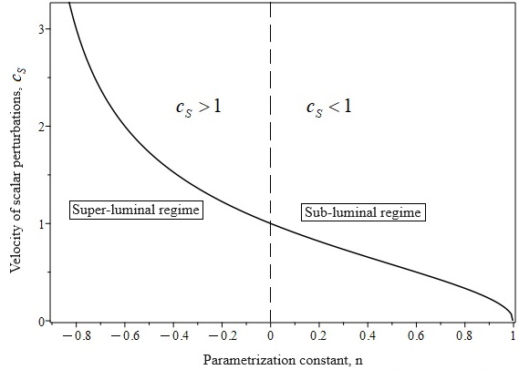
Figure 1: The dependence of the velocity of scalar perturbations from the value of the parametrization constant $n$.

The difference in propagation velocities of scalar and tensor perturbations leads to the fact that the Hubble radius was crossed by them in different wavelengths, namely

$$c_{S}k_{S}=aH,~{}~{}~{}~{}k_{S}=\frac{2\pi a}{\lambda_{S}},$$ (58)

$$c_{T}k_{T}=aH,~{}~{}~{}k_{T}=\frac{2\pi a}{\lambda_{T}},$$ (59)

$$\frac{c_{S}}{c_{T}}=\frac{k_{T}}{k_{S}}=\frac{\lambda_{S}}{\lambda_{T}}=\sqrt{\frac{1-n}{1+n}},$$ (60)

Whereas, in case of the minimal coupling for which $c_{S}=c_{T}=1$, the wavelengths of scalar and tensor perturbations are equal ($\lambda_{S}=\lambda_{T}$). For the case $F=(H/\lambda)^{n}$, from Eq. (50), we obtain

$$Q_{S}=-(1+n)\frac{\dot{H}}{H^{2}}\left(\frac{H}{\lambda}\right)^{n}$$

$$=(1+n)\left(\frac{H}{\lambda}\right)^{n}\epsilon>0,$$ (61)

$$Q_{T}=\frac{1}{4}F=\frac{1}{4}\left(\frac{H}{\lambda}\right)^{n}>0.$$ (62)

The conditions $Q_{S}>0$ and $Q_{T}>0$ indicate that there are no Laplacian instabilities and ghosts in these models [30]. for $F=(H/\lambda)^{n}$, the slow-roll parameters Eqs. (51)–(52) can be related as,

$$\epsilon_{s}=(1-n)\epsilon,~{}~{}~{}~{}~{}~{}\delta_{F}=-n\epsilon,$$

$$\eta_{s}=-2\delta+2\epsilon,~{}~{}~{}~{}~{}~{}s=0.$$ (63)

Thus, the cosmological perturbations (45)–(49) parameters can be written as

$${\mathcal{P}}_{S}=\frac{(2-n)H^{2-n}_{\ast}}{8\pi^{2}(1-n^{2})\sqrt{\frac{1-n}{1+n}}\,\epsilon_{\ast}},$$ (67)

$${\mathcal{P}}_{T}=\frac{2\lambda^{n}}{\pi^{2}}H^{2-n}_{\ast},$$

$$n_{S}-1=(n-4)\epsilon_{\ast}+2\delta_{\ast},$$

$$r=16(1-n)\sqrt{\frac{1-n}{1+n}}\,\epsilon_{\ast},$$

$$n_{T}=-(2-n)\epsilon_{\ast}.$$ (68)

For the case of the minimal coupling, we obtain

$$\tilde{{\mathcal{P}}}_{S}=\frac{h^{2}_{\ast}}{8\pi^{2}\,\tilde{\epsilon}_{\ast}},$$ (69)

$$\tilde{{\mathcal{P}}}_{T}=\frac{2h^{2}_{\ast}}{\pi^{2}},$$ (70)

$$\tilde{n}_{S}-1=-4\tilde{\epsilon}_{\ast}+2\tilde{\delta}_{\ast},$$ (71)

$$\tilde{r}=16\tilde{\epsilon}_{\ast},$$ (72)

$$\tilde{n}_{T}=-2\tilde{\epsilon}_{\ast}.$$ (73)

All parameters of cosmological perturbations are considered at the crossing of the Hubble radius ($k=aH$ and $\tilde{k}=\tilde{a}h$ for some cosmic times $\tilde{t}=\tilde{t}_{\ast}$ and $t=t_{\ast}$, where $t_{\ast}\neq\tilde{t}_{\ast}$ and, correspondingly, $H^{n+1}_{\ast}\neq h_{\ast}$).

Since both minimal and non-minimal coupling cosmological models satisfy condition (42), the relation between the cosmic times of the crossing of the Hubble radius $\xi=\left(t_{\ast}/\tilde{t}_{\ast}\right)$ can be obtained from the equation for certain inflationary models

$${\mathcal{P}}_{S}=\tilde{{\mathcal{P}}}_{S}=2.1\times 10^{-9},$$ (74)

where $\xi=1$ for the case $n=0$.

Since condition (42) can always be satisfied by choosing the time of crossing the Hubble radius or model’s parameters, the spectral index of scalar perturbations and the tensor-scalar ratio as the main parameters necessary for verifying inflationary models by observational constraints (43)–(44). Also, in accordance with restrictions (57), condition $\epsilon_{\ast}>0$ and expression (68), on has red tilt tensor spectrum $n_{T}<0$ for arbitrary cosmological models under consideration.

Further the expressions for the slow-roll parameters (32)–(35) leads to the following relation

$$\frac{\delta}{\epsilon}=(1+n)\frac{\tilde{\delta}}{\tilde{\epsilon}}-\frac{n}{2}.$$ (75)

Since relation (75) must be satisfied for any cosmic times, we get following conditions

$$\tilde{\delta}/\tilde{\epsilon}=constant,$$ (76)

$$\delta/\epsilon=constant,$$ (77)

which restrict the possible types of inflationary models.

VI Inflationary models with linear dependence, $r\sim(1-n_{S})$

Now we will consider the dependence of the tensor-scalar ratio on the spectral index of scalar perturbations $r=r(1-n_{S})$. Since the value of the spectral index of scalar perturbations, $n_{S}\simeq 0.97$ and $1-n_{S}\simeq 0.03\ll 1$, we can write the dependence $r=r(1-n_{S})$ as follows,

$$r=\sum^{\infty}_{k=0}\beta_{k}(1-n_{S})^{k}=\beta_{0}+\beta_{1}(1-n_{S})+$$

$$\beta_{2}(1-n_{S})^{2}+...,$$ (78)

where $(1-n_{S})\ll 1$ is the small parameter of expansion and $\beta_{k}$ are the constant coefficients.

Since, the zeroth order term in this expansion $r(0)=\beta_{0}=0$ from condition $r(n_{S}=1)=0$ corresponding to the flat Harrison-Zel’dovich spectrum [55, 56], we can rewrite expression (VI) in the following form

$$r=\sum^{\infty}_{k=1}\beta_{k}(1-n_{S})^{k}=\beta_{1}(1-n_{S})$$

$$+\beta_{2}(1-n_{S})^{2}+...$$ (79)

The first term in expression (VI) makes the main contribution to the value of the tensor-scalar ratio. Thus, we can consider the dependence $r=r(1-n_{S})$ with a reasonable degree of accuracy at the first order

$$r\simeq\beta_{1}(1-n_{S}),$$ (80)

to analyze the influence of non-minimal coupling on the parameters of inflationary models.

To obtain this dependence, we consider the inflationary models with minimal coupling and constant relation between slow-roll parameters during inflation

$$\frac{\tilde{\delta}}{\tilde{\epsilon}}=\frac{\tilde{\delta}_{\ast}}{\tilde{\epsilon}_{\ast}}=constant.$$ (81)

After substituting relation (81) into (71)–(72), we obtain a linear relationship between the tensor-scalar ratio and the spectral index of scalar perturbations

$$\tilde{r}=\tilde{\beta}_{1}(1-\tilde{n}_{S}).$$ (82)

Also, based on expressions (19), (28) and (34)–(35), we can express the slow-roll parameters in terms of potential in the slow-roll approximation [2]

$$\tilde{\epsilon}=-\frac{\dot{h}}{h^{2}}=2\left(\frac{h_{,\phi}}{h}\right)^{2}\simeq\frac{1}{2}\left(\frac{\tilde{V}_{,\phi}}{\tilde{V}}\right)^{2},$$ (83)

$$\tilde{\delta}=-\frac{\ddot{h}}{2\dot{h}h}=2\frac{h_{,\phi\phi}}{h}\simeq\frac{\tilde{V}_{,\phi\phi}}{\tilde{V}}-\frac{1}{2}\left(\frac{\tilde{V}_{,\phi}}{\tilde{V}}\right)^{2},$$ (84)

where we use the following relations

$$\dot{h}=-2h^{2}_{,\phi},~{}~{}~{}~{}~{}\ddot{h}=8h^{2}_{,\phi}h_{,\phi\phi},~{}~{}~{}~{}~{}h\simeq\left(\frac{V}{3}\right)^{1/2}.$$ (85)

Thus, from condition (81) and equations (83)–(84), we obtain two types of inflationary potential:

$$\tilde{V}(\phi)\sim\phi^{p},~{}~{}~{}~{}~{}~{}~{}~{}~{}~{}~{}~{}~{}~{}~{}~{}~{}{\text{f}or}~{}~{}~{}\tilde{\delta}/\tilde{\epsilon}\neq 1,$$ (86)

$$\tilde{V}(\phi)\sim\exp(-\alpha\phi),~{}~{}~{}~{}{\text{f}or}~{}~{}~{}\tilde{\delta}/\tilde{\epsilon}=1.$$ (87)

where $p$ and $\alpha$ are a some constants.

Models of cosmological inflation based on these potentials have been considered previously in a large number of papers (see, for example, in [57, 58, 59, 60, 61, 62, 63]).

Also, from (29), (32)–(33) and (85), we obtain the following expressions for the slow-roll parameters for the case of non-minimal coupling

$$\epsilon=\frac{2\left(\frac{d}{d\phi}h\left(\phi\right)\right)^{2}h\left(\phi\right)^{-\frac{2+n}{1+n}}}{1+n},$$ (88)

$$\delta=-\frac{2n\left(\frac{d}{d\phi}h\left(\phi\right)\right)^{2}h\left(\phi\right)^{-\frac{2+n}{1+n}}}{2+2n}$$

$$+2\left(\frac{d^{2}}{d\phi^{2}}h\!\left(\phi\right)\right)h\left(\phi\right)^{-\frac{1}{1+n}},$$ (89)

$$h\left(\phi\right)\simeq\left(\frac{\lambda^{n}}{3}V\left(\phi\right)\right)^{\frac{1+n}{2+n}}.$$ (90)

Using these expressions, we will check the compliance with condition $\delta/\epsilon=const$ in the slow-roll approximation, since relation (75) was obtained for exact expressions of the slow-roll parameters.

VI.1 Inflationary models with power-law potential and minimal coupling

Now, we consider the inflationary model with power-law potential [57, 58, 59, 60, 61, 62, 63]

$$\tilde{V}(\phi)=\tilde{V}_{0}\phi^{p},$$ (91)

where $\tilde{V}_{0}$ and $p$ are a some constants.

From (83)–(84), we obtain

$$\tilde{\epsilon}=\frac{p^{2}}{2\phi^{2}}>0,$$ (92)

$$\frac{\tilde{\delta}}{\tilde{\epsilon}}=\frac{\tilde{\delta}_{\ast}}{\tilde{\epsilon}_{\ast}}=\left(\frac{p-2}{p}\right)=const.$$ (93)

Since the slow-roll parameters (92)–(93) contain an unknown arbitrary constant $p$, in this case, it is necessary to obtain an additional dependence of the slow-roll parameters on the e-folds number $\tilde{N}$.

Firstly, we define the value of the scalar field at the end of inflation $\phi=\phi_{e}$. From condition $\epsilon=1$ and expression (92) we obtain

$$\phi^{2}_{e}=\frac{p^{2}}{2}.$$ (94)

Secondly, we define the e-folds number between the crossing of Hubble radius and end of inflation [1, 2]

$$\tilde{N}=\int^{\tilde{t}_{e}}_{\tilde{t}_{\ast}}h(t)dt=\int^{\phi_{e}}_{\phi_{\ast}}\frac{h}{\dot{\phi}}d\phi=-\frac{1}{2}\int^{\phi_{e}}_{\phi_{\ast}}\frac{h}{h_{,\phi}}d\phi$$

$$\simeq-\int^{\phi_{e}}_{\phi_{\ast}}\frac{V}{V_{,\phi}}d\phi.$$ (95)

Further after substituting (91) into (VI.1), we obtain

$$\tilde{N}\simeq\frac{1}{2p}\left(\phi^{2}_{\ast}-\phi^{2}_{e}\right)=\frac{1}{2p}\left(\phi^{2}_{\ast}-\frac{p^{2}}{2}\right).$$ (96)

Thus from Eq. (96), at Hubble radius crossing, we obtain the value of the scalar field a

$$\phi^{2}_{\ast}=\frac{p}{2}\left(p+4\tilde{N}\right).$$ (97)

From Eqs. (92)–(93) and Eq. (97) also, at Hubble radius, the slow-roll parameters can be obtained as,

$$\tilde{\epsilon}_{\ast}=\frac{p}{p+4\tilde{N}},~{}~{}~{}~{}~{}\tilde{\delta}_{\ast}=\frac{p-2}{p+4\tilde{N}}.$$ (98)

From Eqs. (71)–(72) and Eq. (98) we obtain the following expressions for the spectral tilt of the scalar perturbations and tensor-to-scalar ratio

$$1-\tilde{n}_{S}=\frac{2(p+2)}{p+4\tilde{N}},$$ (99)

$$\tilde{r}=\frac{16p}{p+4\tilde{N}}.$$ (100)

Thus, from equations Eqs. (99)–(100) we obtain following dependencies of the tensor-to-scalar ratio from the spectral index of the scalar perturbations

$$\tilde{r}=\frac{8p}{p+2}(1-\tilde{n}_{S}),$$ (101)

$$\tilde{r}=\frac{16\left[(1-\tilde{n}_{S})\tilde{N}-1\right]}{2\tilde{N}-1}.$$ (102)

Due to the observational value of the spectral tilt of the scalar perturbations $\tilde{n}_{S}=0.9663\pm 0.0041$ for a fairly wide range of the e-folds number $50<\tilde{N}<70$, from (102) we obtain $0.08<\tilde{r}<0.20$. Thus, for the minimal coupling, these models don’t correspond to the observational constraint (44).

Also, from expression (99), we obtain:

$$p_{min}(\tilde{n}_{S}=0.9704,\tilde{N}=50)\simeq 1,$$ (103)

$$p_{max}(\tilde{n}_{S}=0.9622,\tilde{N}=70)\simeq 3.34.$$ (104)

Thus, in the slow-roll approximation, we can estimate the values of the parameter $p$ as $1<p<3.4$.

VI.2 Inflationary models with power-law potential and non-minimal coupling

Now, we estimate the influence of non-minimal coupling between the scalar field and torsion on the cosmological parameters. From Eqs. (40)–(41) and Eq. (91) we obtain the following expressions for the potential and non-minimal coupling function

$$V(\phi)\simeq V_{0}\phi^{k},$$ (105)

$$F(\phi)\simeq F_{0}\phi^{m},$$ (106)

where

$$V_{0}=\frac{6(1+n)}{(2-n)}\left(\frac{\tilde{V}_{0}}{3}\right)^{\frac{2+n}{2(1+n)}},~{}~{}~{}k=\frac{p(2+n)}{2(1+n)},$$ (107)

$$F_{0}=\frac{2(1+n)}{(2-n)}\left(\frac{\tilde{V}_{0}}{3}\right)^{\frac{n}{2(1+n)}},~{}~{}~{}m=\frac{pn}{2(1+n)}.$$ (108)

After substituting Eq.(105) and Eq. (107) into Eqs. (88)–(90) we obtain

$$\frac{\delta}{\epsilon}=\frac{\delta_{\ast}}{\epsilon_{\ast}}=(1+n)\left(\frac{p-2}{p}\right)-\frac{n}{2}=const,$$ (109)

that coincides with relation (75).

Also, from Eqs. (67)–(67) and Eq. (109) we get following dependence tensor-to-scalar ratio from spectral tilt of the scalar perturbations

$$r=\frac{8p\sqrt{\frac{1-n}{1+n}}(1-n)(1-n_{S})}{2(1+n)+p(1-n)}.$$ (110)

For $n=0$ this dependence is reduced to Eq. (101).

Further, taking into account the observational constraint $r<0.032$ and restrictions Eqs. (103)–(104) for the same observational values of spectral tilt $\tilde{n}_{S}=n_{S}=0.9663\pm 0.0041$, from Eq. (110) we obtain following constraints on the parametrization constant

$$0.35<n<1,$$ (111)

corresponding to the verifiable inflationary models with potential Eq. (105).

Also, we get the following possible values of the velocity of the scalar perturbations $0<c_{S}<0.7$ from expression (56). Thus, in the sub-luminal regime of the propagation of scalar perturbations, this model corresponds to the observational constraints (43)–(44). Therefore, for the case of scalar-torsion gravity, inflationary models with power-law potential can be verified by observational constraints on the values of the parameters of cosmological perturbations.

VI.3 Inflationary models with exponential potential

Now, we consider the inflationary model with exponential potential [57, 58, 59]

$$\tilde{V}(\phi)=\tilde{V}_{0}\exp(-\alpha\phi),$$ (112)

where $\tilde{V}_{0}$ and $\alpha$ are a some positive constants.

From Eqs. (83)–(84), we obtain

$$\tilde{\epsilon}=\tilde{\epsilon}_{\ast}=\frac{\alpha^{2}}{2}>0,$$ (113)

$$\frac{\tilde{\delta}}{\tilde{\epsilon}}=\frac{\tilde{\delta}_{\ast}}{\tilde{\epsilon}_{\ast}}=1.$$ (114)

Since relation (114) doesn’t contain additional constant parameters, we can immediately determine the dependence of the tensor-scalar ratio on the spectral index of scalar perturbations. This dependence will be valid for any e-fold number including $50<\tilde{N}<70$.

Thus, from Eqs. (71)–(72) and Eq. (114) we obtain

$$\tilde{r}=8(1-\tilde{n}_{S}).$$ (115)

After substituting $\tilde{n}_{S}\simeq 0.97$ into Eq. (115) one can have $\tilde{r}\simeq 0.24$. Thus, the inflationary model with exponential potential (112) doesn’t satisfy the observational constraint Eq. (44) for the case of minimal coupling. For the case of non-minimal coupling, from equations Eqs. (40)–(41) and Eq. (112) we get

$$V(\phi)\simeq V_{0}\exp\left(-\frac{\alpha(2+n)}{2(1+n)}\phi\right),$$ (116)

$$F(\phi)\simeq F_{0}\exp\left(-\frac{n\phi}{2(1+n)}\right),$$ (117)

where

$$V_{0}=\frac{6(1+n)}{(2-n)}\left(\frac{\tilde{V}_{0}}{3}\right)^{\frac{2+n}{2(1+n)}},$$ (118)

$$F_{0}=\frac{2(1+n)}{(2-n)}\left(\frac{\tilde{V}_{0}}{3}\right)^{\frac{2+n}{2(1+n)}}.$$ (119)

After substituting (116) into (88)–(90) we obtain

$$\frac{\delta}{\epsilon}=\frac{\delta_{\ast}}{\epsilon_{\ast}}=1+\frac{n}{2}=const,$$ (120)

that coincides with relation (75).

Further, from (67)–(67) and (120) we obtain

$$r=8\sqrt{\frac{1-n}{1+n}}\,(1-n_{S}).$$ (121)

Thus, for $n_{S}\simeq 0.97$ and $r<0.032$, from (121) we get $0<n<0.965$. Also, for $0<n<0.965$ corresponding velocity of the scalar perturbations (56) takes the values $0<c_{S}<0.13$.

Therefore, this inflationary model is verified by observational constraints only for the case of a very strong influence of the non-minimal coupling on the velocity of propagation of the scalar perturbations. For this reason, the inflationary models with power-law potential seem more realistic.

VII Conclusion

We testify the influence of non-minimal coupling between scalar field and torsion on the cosmological parameters based on power-law relationship between coupling function and Hubble parameter $F=(H/\lambda)^{n}$. The novelty of proposed approach is the possibility of a model-independent assessment of non-minimal coupling effect on cosmological parameters. The non-minimal coupling influence was parameterized by one constant parameter $n$. Also, we found restrictions on the value of parametrization constant $-1<n<1$. The influence of non-minimal coupling on cosmological dynamics, scalar field potential, and cosmological perturbations parameters was assessed by this approach.

We have shown that inflationary models implying a linear relationship between the tensor-scalar ratio and spectral index of scalar perturbations can be verified by observational constraints on the values of cosmological perturbation parameters by influence of the non-minimal coupling between scalar field and torsion. These influence leads to a sub-luminal regime of the propagation of scalar perturbations and a decrease in the value of the tensor-scalar ratio for inflationary models under consideration.

Further development of the proposed approach is associated with its generalization to the case of the violation of relations $H=h^{1/(1+n)}$ and $\delta/\epsilon=const$. This generalization leads to a wider class of cosmological models including models with a super-luminal velocity of propagation of scalar perturbations and increasing tensor-to-scalar ratio.

References

References

- [1] D. Baumann and L. McAllister, Inflation and String Theory. Cambridge Monographs on Mathematical Physics. Cambridge University Press, 5, 2015. arXiv:1404.2601 [hep-th].
- [2] S. Chervon, I. Fomin, V. Yurov, and A. Yurov, Scalar Field Cosmology, vol. 13 of Series on the Foundations of Natural Science and Technology. WSP, Singapur, 2019.
- [3] P. J. Steinhardt and D. Wesley, “Dark Energy, Inflation and Extra Dimensions,” Phys. Rev. D 79 (2009) 104026, arXiv:0811.1614 [hep-th].
- [4] T. Clifton, P. G. Ferreira, A. Padilla, and C. Skordis, “Modified Gravity and Cosmology,” Phys. Rept. 513 (2012) 1–189, arXiv:1106.2476 [astro-ph.CO].
- [5] S. Nojiri, S. D. Odintsov, and V. K. Oikonomou, “Modified Gravity Theories on a Nutshell: Inflation, Bounce and Late-time Evolution,” Phys. Rept. 692 (2017) 1–104, arXiv:1705.11098 [gr-qc].
- [6] M. Ishak, “Testing General Relativity in Cosmology,” Living Rev. Rel. 22 (2019) no. 1, 1, arXiv:1806.10122 [astro-ph.CO].
- [7] S. Shankaranarayanan and J. P. Johnson, “Modified theories of gravity: Why, how and what?,” Gen. Rel. Grav. 54 (2022) no. 5, 44, arXiv:2204.06533 [gr-qc].
- [8] V. C. de Andrade, L. C. T. Guillen, and J. G. Pereira, “Gravitational energy momentum density in teleparallel gravity,” Phys. Rev. Lett. 84 (2000) 4533–4536, arXiv:gr-qc/0003100.
- [9] H. I. Arcos and J. G. Pereira, “Torsion gravity: A Reappraisal,” Int. J. Mod. Phys. D 13 (2004) 2193–2240, arXiv:gr-qc/0501017.
- [10] C.-Q. Geng, C.-C. Lee, E. N. Saridakis, and Y.-P. Wu, ““Teleparallel” dark energy,” Phys. Lett. B 704 (2011) 384–387, arXiv:1109.1092 [hep-th].
- [11] K. Bamba, R. Myrzakulov, S. Nojiri, and S. D. Odintsov, “Reconstruction of gravity: Rip cosmology, finite-time future singularities and thermodynamics,” Phys. Rev. D 85 (2012) 104036, arXiv:1202.4057 [gr-qc].
- [12] K. Bamba, S. D. Odintsov, and D. Sáez-Gómez, “Conformal symmetry and accelerating cosmology in teleparallel gravity,” Phys. Rev. D 88 (2013) 084042, arXiv:1308.5789 [gr-qc].
- [13] K. Bamba, S. Nojiri, and S. D. Odintsov, “Trace-anomaly driven inflation in gravity and in minimal massive bigravity,” Phys. Lett. B 731 (2014) 257–264, arXiv:1401.7378 [gr-qc].
- [14] M. A. Skugoreva, E. N. Saridakis, and A. V. Toporensky, “Dynamical features of scalar-torsion theories,” Phys. Rev. D 91 (2015) 044023, arXiv:1412.1502 [gr-qc].
- [15] L. Jarv and A. Toporensky, “General relativity as an attractor for scalar-torsion cosmology,” Phys. Rev. D 93 (2016) no. 2, 024051, arXiv:1511.03933 [gr-qc].
- [16] A. Awad, W. El Hanafy, G. G. L. Nashed, S. D. Odintsov, and V. K. Oikonomou, “Constant-roll Inflation in Teleparallel Gravity,” JCAP 07 (2018) 026, arXiv:1710.00682 [gr-qc].
- [17] M. Krssak, R. J. van den Hoogen, J. G. Pereira, C. G. Böhmer, and A. A. Coley, “Teleparallel theories of gravity: illuminating a fully invariant approach,” Class. Quant. Grav. 36 (2019) no. 18, 183001, arXiv:1810.12932 [gr-qc].
- [18] M. Hohmann, L. Järv, and U. Ualikhanova, “Covariant formulation of scalar-torsion gravity,” Phys. Rev. D 97 (2018) no. 10, 104011, arXiv:1801.05786 [gr-qc].
- [19] M. Gonzalez-Espinoza and G. Otalora, “Cosmological dynamics of dark energy in scalar-torsion gravity,” Eur. Phys. J. C 81 (2021) no. 5, 480, arXiv:2011.08377 [gr-qc].
- [20] L. Järv and J. Lember, “Global Portraits of Nonminimal Teleparallel Inflation,” Universe 7 (2021) no. 6, 179, arXiv:2104.14258 [gr-qc].
- [21] L. K. Duchaniya, S. A. Kadam, J. L. Said, and B. Mishra, “Dynamical systems analysis in gravity,” The European Physical Journal C 83 (2023) no. 1, , arXiv:2209.03414 [gr-qc].
- [22] L. K. Duchaniya, B. Mishra, and J. L. Said, “Noether symmetry approach in scalar-torsion gravity,” The European Physical Journal C 83 (2023) no. 7, , arXiv:2210.11944 [gr-qc].
- [23] S. A. Kadam, B. Mishra, and J. Said Levi, “Teleparallel scalar-tensor gravity through cosmological dynamical systems,” Eur. Phys. J. C 82 (2022) no. 8, 680, arXiv:2205.04231 [gr-qc].
- [24] A. Paliathanasis, “ symmetry in teleparallel dark energy,” Eur. Phys. J. Plus 136 (2021) no. 6, 674, arXiv:2105.08527 [gr-qc].
- [25] A. Paliathanasis, “Complex scalar fields in scalar-tensor and scalar-torsion theories,” Mod. Phys. Lett. A 37 (2022) no. 25, 2250168, arXiv:2210.04177 [gr-qc].
- [26] G. Leon, A. Paliathanasis, E. N. Saridakis, and S. Basilakos, “Unified dark sectors in scalar-torsion theories of gravity,” Phys. Rev. D 106 (2022) no. 2, 024055, arXiv:2203.14866 [gr-qc].
- [27] S.-H. Chen, J. B. Dent, S. Dutta, and E. N. Saridakis, “Cosmological perturbations in f(T) gravity,” Phys. Rev. D 83 (2011) 023508, arXiv:1008.1250 [astro-ph.CO].
- [28] A. Golovnev and T. Koivisto, “Cosmological perturbations in modified teleparallel gravity models,” JCAP 11 (2018) 012, arXiv:1808.05565 [gr-qc].
- [29] S. Raatikainen and S. Rasanen, “Higgs inflation and teleparallel gravity,” JCAP 12 (2019) 021, arXiv:1910.03488 [gr-qc].
- [30] M. Gonzalez-Espinoza, G. Otalora, N. Videla, and J. Saavedra, “Slow-roll inflation in generalized scalar-torsion gravity,” JCAP 08 (2019) 029, arXiv:1904.08068 [gr-qc].
- [31] M. Gonzalez-Espinoza and G. Otalora, “Generating primordial fluctuations from modified teleparallel gravity with local Lorentz-symmetry breaking,” Phys. Lett. B 809 (2020) 135696, arXiv:2005.03753 [gr-qc].
- [32] Y.-F. Cai, S. Capozziello, M. De Laurentis, and E. N. Saridakis, “f(T) teleparallel gravity and cosmology,” Rept. Prog. Phys. 79 (2016) no. 10, 106901, arXiv:1511.07586 [gr-qc].
- [33] L. K. Duchaniya, S. V. Lohakare, B. Mishra, and S. K. Tripathy, “Dynamical stability analysis of accelerating f(T) gravity models,” Eur. Phys. J. C 82 (2022) no. 5, 448, arXiv:2202.08150 [gr-qc].
- [34] L. K. Duchaniya, K. Gandhi, and B. Mishra, “Attractor behavior of modified gravity and the cosmic acceleration,” Physics of the Dark Universe 44 (2024) 101461, arXiv:2303.09076 [gr-qc].
- [35] C. Li, Y. Cai, Y.-F. Cai, and E. N. Saridakis, “The effective field theory approach of teleparallel gravity, gravity and beyond,” JCAP 10 (2018) 001, arXiv:1803.09818 [gr-qc].
- [36] I. V. Fomin, S. V. Chervon, and A. V. Tsyganov, “Generalized scalar-tensor theory of gravity reconstruction from physical potentials of a scalar field,” Eur. Phys. J. C 80 (2020) no. 4, 350, arXiv:2004.08544 [gr-qc].
- [37] I. Fomin and S. Chervon, “Exact and Slow-Roll Solutions for Exponential Power-Law Inflation Connected with Modified Gravity and Observational Constraints,” Universe 6 (2020) no. 11, 199.
- [38] I. V. Fomin, S. V. Chervon, A. N. Morozov, and I. S. Golyak, “Relic gravitational waves in verified inflationary models based on the generalized scalar-tensor gravity,” Eur. Phys. J. C 82 (2022) no. 7, 642.
- [39] I. V. Fomin and S. V. Chervon, “Exact inflation in Einstein-Gauss-Bonnet gravity,” Grav. Cosmol. 23 (2017) no. 4, 367–374, arXiv:1704.03634 [gr-qc].
- [40] I. V. Fomin and S. V. Chervon, “A new approach to exact solutions construction in scalar cosmology with a Gauss–Bonnet term,” Mod. Phys. Lett. A 32 (2017) no. 25, 1750129, arXiv:1704.07786 [gr-qc].
- [41] I. V. Fomin, “Cosmological Inflation with Einstein-Gauss-Bonnet Gravity,” Phys. Part. Nucl. 49 (2018) no. 4, 525–529.
- [42] I. Fomin, “Gauss-Bonnet term corrections in scalar field cosmology,” Eur. Phys. J. C 80 (2020) no. 12, 1145, arXiv:2004.08065 [gr-qc].
- [43] S. V. Chervon and I. V. Fomin, “Reconstruction of Scalar-Torsion Gravity Theories from the Physical Potential of a Scalar Field,” Symmetry 15 (2023) no. 2, 291.
- [44] M. Giovannini, “Primordial backgrounds of relic gravitons,” Prog. Part. Nucl. Phys. 112 (2020) 103774, arXiv:1912.07065 [astro-ph.CO].
- [45] E. H. Tanin and T. Tenkanen, “Gravitational wave constraints on the observable inflation,” JCAP 01 (2021) 053, arXiv:2004.10702 [astro-ph.CO].
- [46] S. D. Odintsov and V. K. Oikonomou, “Amplification of Primordial Gravitational Waves by a Geometrically Driven non-canonical Reheating Era,” Fortsch. Phys. 70 (2022) no. 5, 2100167, arXiv:2203.10599 [gr-qc].
- [47] Planck Collaboration, N. Aghanim et al., “Planck 2018 results. VI. Cosmological parameters,” Astron. Astrophys. 641 (2020) A6, arXiv:1807.06209 [astro-ph.CO]. [Erratum: Astron.Astrophys. 652, C4 (2021)].
- [48] M. Tristram et al., “Improved limits on the tensor-to-scalar ratio using BICEP and Planck data,” Phys. Rev. D 105 (2022) no. 8, 083524, arXiv:2112.07961 [astro-ph.CO].
- [49] V. Mukhanov, Physical Foundations of Cosmology. Cambridge University Press, Oxford, 2005.
- [50] V. F. Mukhanov and A. Vikman, “Enhancing the tensor-to-scalar ratio in simple inflation,” JCAP 02 (2006) 004, arXiv:astro-ph/0512066.
- [51] E. Babichev, V. Mukhanov, and A. Vikman, “k-Essence, superluminal propagation, causality and emergent geometry,” JHEP 02 (2008) 101, arXiv:0708.0561 [hep-th].
- [52] A. De Felice and T. Suyama, “Vacuum structure for scalar cosmological perturbations in Modified Gravity Models,” JCAP 06 (2009) 034, arXiv:0904.2092 [astro-ph.CO].
- [53] S. Koh, B.-H. Lee, and G. Tumurtushaa, “Reconstruction of the Scalar Field Potential in Inflationary Models with a Gauss-Bonnet term,” Phys. Rev. D 95 (2017) no. 12, 123509, arXiv:1610.04360 [gr-qc].
- [54] S. Mironov, V. Rubakov, and V. Volkova, “Superluminality in DHOST theory with extra scalar,” JHEP 04 (2021) 035, arXiv:2011.14912 [hep-th].
- [55] E. R. Harrison, “Fluctuations at the threshold of classical cosmology,” Phys. Rev. D 1 (1970) 2726–2730.
- [56] Y. B. Zeldovich, “Gravitational instability: An Approximate theory for large density perturbations,” Astron. Astrophys. 5 (1970) 84–89.
- [57] J. Martin, C. Ringeval, and V. Vennin, “Encyclopædia Inflationaris,” Phys. Dark Univ. 5-6 (2014) 75–235, arXiv:1303.3787 [astro-ph.CO].
- [58] J. Martin, C. Ringeval, R. Trotta, and V. Vennin, “The Best Inflationary Models After Planck,” JCAP 03 (2014) 039, arXiv:1312.3529 [astro-ph.CO].
- [59] O. Grøn, “Predictions of Spectral Parameters by Several Inflationary Universe Models in Light of the Planck Results,” Universe 4 (2018) no. 2, 15.
- [60] S. S. Mishra, V. Sahni, and A. V. Toporensky, “Initial conditions for Inflation in an FRW Universe,” Phys. Rev. D 98 (2018) no. 8, 083538, arXiv:1801.04948 [gr-qc].
- [61] N. A. Avdeev and A. V. Toporensky, “Ruling Out Inflation Driven by a Power Law Potential: Kinetic Coupling Does Not Help,” Grav. Cosmol. 28 (2022) no. 4, 416–419, arXiv:2203.14599 [gr-qc].
- [62] S. D. Odintsov, V. K. Oikonomou, I. Giannakoudi, F. P. Fronimos, and E. C. Lymperiadou, “Recent Advances in Inflation,” Symmetry 15 (2023) no. 9, 1701, arXiv:2307.16308 [gr-qc].
- [63] S. D. Odintsov, S. D’Onofrio, and T. Paul, “Entropic Inflation in Presence of Scalar Field,” Universe 10 (2024) no. 1, 4, arXiv:2312.13587 [gr-qc].