Spacetime representation of quantum mechanics and a proposal for quantum gravity
Hong Wanga, Jin Wangb,111jin.wang.1@stonybrook.edu
aState Key Laboratory of Electroanalytical Chemistry, Changchun Institute of Applied Chemistry, Chinese Academy of Sciences, Changchun 130022, China
bDepartment of Chemistry and Department of Physics and Astronomy, State University of New York at Stony Brook, NY 11794, USA
In conventional path integral quantum mechanics, the integral variables are the canonical variables of Hamiltonian mechanics. We show that these integral variables can be transformed into the spacetime metric, leading to a new representation of quantum mechanics. We show that the wave-particle duality can be interpreted as the uncertainty of spacetime for the particle. Summarizing all possible trajectories in conventional path integral quantum mechanics can be transformed into the summation of all possible spacetime metrics. We emphasize that in conventional quantum gravity, it is possible that the classical matter fields correspond to the quantum spacetime. We argue that this is not quite reasonable and propose a new path integral quantum gravity model based on the new interpretation of wave-particle duality. In this model, the aforementioned drawback of conventional quantum gravity naturally disappears.
1 Introduction
Quantum mechanics has been studied for nearly a century. Despite ongoing debates regarding the interpretation of the wave function, it has become one of the greatest theories. Quantum theories for the weak, strong and electromagnetic interactions have been successfully developed. These theories collectively constitute the renowned Standard Model of particle physics. However, a self-consistent quantum theory of gravity is still lacking [1, 2]. Therefore, it is significant to make new attempts to construct a theory of quantum gravity.
There are two equivalent methods for quantizing a system: the path integral and canonical quantization. In path integral quantum mechanics, to calculate the transition amplitude, one must sum up all possible trajectories. The trajectory with the minimum action is the classical trajectory. For a free particle, it is a straight line. Other trajectories are not straight lines and do not satisfy the Hamilton-Jacobi equation. Only the classical trajectory corresponds clearly to a dynamical equation (Hamilton-Jacobi equation). Thus, the classical trajectory possesses a special status. However, it may be more natural to consider all trajectories as solutions of some dynamical equations. What is this relevant dynamical equation? Is this idea feasible, and what implications does it have for quantum mechanics?
In this work, we show that different trajectories in the path integral can be regarded as solution of the Hamilton-Jacobi equation in different spacetimes. For the free particle, different trajectories in the path integral can be interpreted as the geodesics in different spacetimes. We find that the integration over all possible trajectories in the path integral quantum mechanics can be transformed into the integration over various spacetime metrics. This results in the spacetime representation of quantum mechanics. We demonstrate that the wave-particle duality can be interpreted as the uncertainty of the spacetime structure for the microscopic particle. Thus, the quantum characteristics of any system can be attributed to the uncertainty of the spacetime structure. We show that in the spacetime representation, when using the path integral to quantize any system, one only needs to set the spacetime metric as the integral variable.
In conventional path integral quantum gravity, classical matter fields may correspond to the quantum spacetime [3]. We demonstrate that this is not quite reasonable. Based on the new interpretation of the wave-particle duality, we propose that in path integral quantum gravity, only the spacetime metric should be considered as the integral variable. By adopting this proposal, the aforementioned problem in quantum gravity can be easily circumvented. Throughout this study, we work in units where .
2 Spacetime representation of quantum mechanics
2.1 A single particle
In quantum mechanics, there are still conceptual puzzles regarding the wave-particle duality and the wave function. The evolution of the wave function is governed by the Schrödinger equation, which can be expressed in various representations. Different representations are connected through a unitary transformation. In this section, we will explore the possibility of a spacetime representation in quantum mechanics, which may help to understand the wave-particle duality and the wave function.
The spacetime coordinates can be chosen arbitrarily. Cartesian coordinates are convenient for our illustration. We will use symbols , , , … to represent Cartesian coordinates. Other coordinates will be denoted by different symbols, such as , , …. In Cartesian coordinates, the spacetime metric is
| (1) |
Various spacetimes correspond to different . When the spacetime is flat, Cartesian coordinates imply that , where represents the Minkowski metric.
For simplicity, we start by examining a relativistic free particle in a curved spacetime. The classical dynamics of the particle are determined by its action, expressed as [4]
| (2) |
where, and represent the rest mass of the particle and the spacetime metric, respectively. Taking , one can obtain the classical dynamical equation (geodesic equation) of the particle as
| (3) |
Here, is the connection. For the torsionless spacetime, .
In a specific spacetime , if the initial state of the particle is fixed, then equation (3) has a unique solution. Changing the metric continuously, the solution may also be changed continuously. Thus, the trajectory of the particle can be seen as a functional of the metric. We formally denote the solution of the geodesic equation (3) as
| (4) |
Equation (3) is a nonlinear equation. It is difficult to give a general solution for the geodesic equation. Thus, the explicitly form of the functional is difficult to specify. However, the conclusions of this work are independent of the detailed form of the functional . We point out that the metric and the solution of equation (3) is not in a one-to-one correspondence. Fixing the metric and the initial state of the particle, there is only one trajectory that satisfies equation (3). Conversely, given the trajectory and the initial state of the particle, there are infinite spacetime metrics are compatible with the trajectory of the particle. In other words, one can not determine the spacetime structure (metric) according to a trajectory of the free particle.
Equation (3) can also be interpreted as a particle moving in a gravitational field. When the gravitational field strength is zero, the trajectory of the particle is a straight line. By changing the gravitational field, the trajectory can take on any curve. Thus, it is reasonable to infer that for any given curve (not violating physical principles), there exists a gravitational field that makes it to become the particle’s trajectory. In other words, given any one physically allowed curve, it can always be embedded into a spacetime where it becomes a geodesic. By changing the local spacetime structure far from the trajectory of the particle, the dynamics of the particle remain unaffected. Hence, for any physically allowed curve, there are infinite types of spacetime where one of the geodesics matches this curve.
In the Minkowski spacetime, according to conventional path integral quantum mechanics, the transition amplitude of a relativistic particle from the initial state to the final state can be written as
| (5) |
Here, represents the normalized constant. represents the summation over all trajectories connecting the initial and final states. The factor represents the length of the trajectory between the initial and final state. The lengths of different trajectories may be different. The classical trajectory is the solution to the Hamilton-Jacobi equation, while all other trajectories do not satisfy the classical dynamical equation.
Every trajectory in the path integral (5) is a possible path of the particle from the initial state to the final state . And each trajectory should be physically allowed. As discussed previously, for any given trajectory in the path integral (5), there exists a spacetime where this trajectory is a geodesic. (This point is crucial for this study. We provide a more rigorous demonstration of this point in the appendix.) Therefore, the length of the trajectory can be written as
| (6) |
The two sides of equation (6) represent two different viewpoints on the same trajectory. On the left hand side, the trajectory is viewed as a curve (not a geodesic) in Minkowski spacetime. On the right hand side, the trajectory is seen as a geodesic in the spacetime . Changing the metric far from the trajectory does not alter the properties of the trajectory. Thus, there exist infinitely many types of that satisfy equation (6).
A simple example is that when calculating the length of a circle defined by , one can view the circle as an ordinary curve in the Euclidean space , and use the formula to calculate its length. One can also regard the circle as a geodesic on the two dimensional sphere surface space , and then use the formula to calculate its length. Thus, one can obtain the equation
| (7) |
The local spacetime structure far away from the circle has no influence on its properties. Thus, one can find infinity types of that satisfy equation (7).
For Minkowski spacetime, only the straight line between the initial state and the final state is the geodesic. In a curved spacetime, it is possible that more than one trajectories in the path integral (5) can be interpreted as the geodesics in the same spacetime. However, in this work, we consistently treat different trajectories in the path integral (5) as geodesics in distinct spacetimes. Each trajectory corresponds to a different spacetime. Thus, the integral over different paths in equation (5) can be transformed into an integral over different metrics. Therefore, using equations (4) and (6), equation (5) can be written as
| (8) |
Here, represents the Jacobian determinant, which is induced by the transformation of the integral variables ().
Noted that for every trajectory , there are infinitely many types of metric that satisfy equation (6). We define these spacetimes as the same class of spacetime and use to denote it. Every trajectory in the path integral (5) corresponds to different classes of spacetime . For a specific spacetime, it belongs to and only belongs to one of the classes . As each trajectory is only counted once in the path integral (5), thus, in each class of spacetime , only one metric contributes to the path integral. However, in equation (8), the integral contains all metrics for every class of spacetime . We need to eliminate the redundant metrics.
In order to eliminate redundant metrics in the path integral (8), only one metric from each class of spacetime should be included in the path integral. In each class of spacetime , every metric is equivalent in terms of the path integral (8). Thus, it is permissible to select any metric from each class arbitrarily. For this purpose, one can introduce a set of gauge conditions
| (9) |
Here, represents the total number of gauge conditions. Similar to the scenario with Yang-Mills gauge fields, the gauge conditions have a certain degree of arbitrariness. As long as the solution to equations (9) can uniquely determine a metric from each class of spacetime , the gauge conditions are considered valid. For every trajectory in the path integral (5), there exists a single metric that satisfies both equations (6) and (9).
According to the Faddeev-Popov method [5, 6], to eliminate the redundant metrics, equation (8) should be modified as
| (10) |
Here, and represent the Faddeev-Popov determinant and the -function, respectively. The Jacobian determinant is determined by equation (4), while the Faddeev-Popov determinant depends on the gauge conditions (9). The conclusions of this work are independent of the explicit form of , and . Thus, we will avoid solving them. This is a challenging issue that needs careful study in the future.
Equation (10) represents a new kind of representation of quantum mechanics. We name it the spacetime representation. Equation (5) is equivalent to equation (10). Thus, the integration over different trajectories can be transformed into integration over various spacetime metrics. Equation (10) indicates that the quantum characteristics of the particle can be attributed to the uncertainty of the spacetime structure for the microscopic particle. In the conventional interpretation of path integral quantum mechanics, only the classical trajectory corresponds to the Hamilton-Jacobi equation. All other trajectories are not solutions of any dynamical equations. Thus, the classical trajectory possesses a special status. However, we argued that for the free particle, all trajectories can be seen as the geodesics in different spacetimes. Thus, different trajectories are solutions of the geodesic equation in different spacetimes. This perspective offers a more natural understanding of these trajectories. In table 1, we outlined the key distinctions between the conventional path integral and the spacetime representation for a single relativistic free particle. When , the microscopic particle becomes a macroscopic object. The coherence disappears and the dynamics of the particle can be described by the classical physics.
According to conventional quantum mechanics, the quantum characteristics of a particle are induced by the wave-particle duality. Thus, equation (10) implies that the wave-particle duality can be interpreted as the uncertainty of the spacetime structure. In addition, one can consider that different metrics in equation (10) correspond to different universes. Thus, integrating over different metrics can be seen as integrating over various universes. Consequently, equation (10) is more clearly associated with the multiverse interpretation of quantum mechanics [7, 8].
| Conventional path integral | Spacetime representation | |
| Partition function | Equation (5) | Equation (10) |
| Integral variable | Particle’s trajectory | Spacetime metric |
| Spacetime structure | Spacetime structure is deterministic (Minkowski spacetime). | Spacetime structure is uncertain for the microscopic particle. |
| Particle’s trajectories | Only the classical trajectory is the solution of the Hamilton-Jacobi equation. All other trajectories in the path integral (5) do not correspond to any dynamical equation. | All trajectories in the path integral (5) are viewed as geodesics in different spacetimes. |
2.2 The general system
In the last subsection, we show that for a free particle, the wave-particle duality can be interpreted as the uncertainty of the spacetime structure for the microscopic particle. It is well known that the non commutative relationship is one of the most fundamental equations in quantum mechanics. Both the wave-particle duality and the non commutative relationship hold true regardless of whether the particle is involved in interactions. In this subsection, we will show that in all scenarios, the wave-particle duality can always be interpreted as the uncertainty of the spacetime structure for the particle. And the path integral for any quantum system can be transformed into an integration over various spacetime metrics.
Usually, a physical system is composed of particles. In the case where the particle number is conserved, the action of the total system can be defined as
| (11) |
Here, represents the total number of the particles. and represent the coordinate and the rest mass of the -th particle, respectively. And represents the interactions between different particles. Taking , one can obtain the classical dynamical equation of the system under general spacetime as
| (12) |
It is evident that when , equation (12) becomes the geodesic equation (3). Generally, when , the trajectory of each particle is not the geodesic of the spacetime .
Specifying the spacetime metric and the initial state of the system, equation (12) has only one solution. This solution represents the trajectories of the particles. We denote this solution as . Similar to the last subsection, intuitively speaking, changing the spacetime metric can lead the trajectories to become any set of curves (physically allowed). Thus, it is reasonable to deduce that by providing any set of curves (composed of physically allowed trajectories), one can find a class of metric in which this set of curves serves as the solution to equation (12).
According to conventional quantum mechanics in Minkowski spacetime (), the transition amplitude of the system defined by equation (11) from the initial state to the final state is
| (13) |
The path integral represents that all possible sets of trajectories are summed over.
We have argued that for any given set of trajectories , it is always possible to embed them into a class of metric where the trajectories satisfy equation (12). Therefore, the integration over different trajectories in equation (LABEL:eq:1.12) can be transformed into an integration over various classes of spacetime metric . Following the similar statements of the last subsection, the path integral (LABEL:eq:1.12) can be transformed into
| (14) |
Here, , and represent the Jacobian determinant, the Faddeev-Popov determinant and the gauge conditions, respectively. represent the number of the gauge conditions. These quantities differ from those of a free particle. Once again, we refrain from explicitly determining their forms in this study.
Equation (LABEL:eq:1.13) is equivalent to equation (LABEL:eq:1.12). Equation (LABEL:eq:1.13) indicates that in a general system, integrating over different trajectories can be transformed into integrating over various spacetime metrics . In equation (LABEL:eq:1.13), the spacetime metric is the only integral variable. Thus, the wave-particle duality can generally be interpreted as the uncertainty of the spacetime structure for microscopic particle. Therefore, it is reasonable to infer that the quantum characteristics of a general system can be ascribed to the uncertainty of the spacetime structure. Moreover, this perspective implies a potential relationship between quantum characteristics and geometric quantities. It is worth noting that the Ryu-Takayanagi formula indicates that the entanglement entropy of the conformal field theory equals the area of the minimal surface [9, 10]. Consequently, the Ryu-Takayanagi formula may support our argument.
It is well known that the most successful theory (up to now) for describing interactions between microscopic particles is quantum field theory. This theory can describe the quantum dynamics of a system whether the particle number is conserved or not. The quantum dynamics of the system defined by equation (11) can also be described by quantum field theory. Thus, the equivalence between equations (LABEL:eq:1.12) and (LABEL:eq:1.13) implies that the path integral over different quantum fields can also be transformed into integration over various spacetime metrics. To illustrate this viewpoint, we will use the scalar field as an example.
The action of a scalar field minimally coupled with the curved spacetime is defined as [11]
| (15) |
Here, and represent the scalar field and the scalar potential, respectively. Taking , one can obtain the classical dynamical equation of the scalar field as [11]
| (16) |
Given the initial state of the scalar field and the spacetime metric , equation (16) has a unique solution. We denote this solution as . By varying the metric , the solution can be transformed into any physically allowed scalar field configuration. Thus, conversely, it is reasonable to infer that given any physically allowed scalar field configuration, one can find a spacetme metric in which this field configuration serves as the solution of equation (16). Therefore, the integration over different field configurations can be transformed into the integration over various metrics.
Following the statements in the last subsection, the partition function of the scalar field in Minkowski spacetime
| (17) |
can be equivalently written as
| (18) |
where, , and represent the Jacobian determinant, the Faddeev-Popov determinant and the gauge conditions, respectively. is the number of the gauge conditions. For the quantum field theory, it seems possible that . In this case, when changing the path integral variable , one does not need to introduce any gauge conditions. However, the conclusions of this work remain unaffected by the specific value of .
We point out that in equation (18), although the path integral is performed over various spacetime metrics, the impact of the matter field on the spacetime structure (the effect of general relativity) is not taken into account. Equation (18) solely indicates that the non commutative relationship can be interpreted as the uncertainty of the spacetime structure for the scalar field . For a field with a non zero spin, there may exist a correlation between the spin and the spacetime torsion [12, 13, 14]. We do not delve into these more complex fields in this study. However, based on our discussions, it is reasonable to deduce that the quantum characteristics of any quantum field can be ascribed to the uncertainty of the spacetime structure.
3 A proposal for the path integral quantum gravity
Although a self-consistent and complete quantum gravity theory is still lacking, there are some exciting attempts to construct the quantum gravity theory, such as string theory, holographic duality, loop quantum gravity, and more [1, 2, 15, 16, 17]. Perhaps the most conservative approach is the path integral quantum gravity
| (19) |
or the canonical quantum gravity
| (20) |
In equation (19), represents the matters, and represents the total action of the system. Equation (20) is the Wheeler-De Witt equation. It is widely believed that the path integral approach (19) and the canonical quantization approach should be equivalent if the Hamiltonian operator is properly defined. We will focus on these two approaches of quantum gravity.
There are some divergence difficulties that have not been fully resolved in the path integral approach [18, 19]. The time problem in the Wheeler-De Witt equation has also not been fully addressed [1, 3, 20, 21]. The aim of this study is not to solve all these well-known problems. Instead, we will demonstrate that there may be another issue present in both the conventional path integral quantum gravity and the canonical quantum gravity. We also propose a solution to circumvent this issue based on our discussions in section 2.
Consider a simple example of the flat () FRW universe. In the conformal time coordinate, the classical spacetime metric is
| (21) |
Here, represents the scale factor. The FRW spacetime is a minisuperspace model. For the minisuperspace model, there is no functional evolution problem [20].
If there is a massless real scalar field minimally coupled with the FRW spacetime, the action of the total system is [3]
| (22) |
On the right hand side of equation (22), the first term is the Einstein-Hilbert action. The second term represents the action of the scalar field. and represent the Ricci scalar and the Gibbons–Hawking–York surface term, respectively.
Combining equations (21) and (22), one can prove that the total Hamiltonian operator of the system (22) can be approximately written as [3]
| (23) |
Here, and represent the coordinate volume and the conjugate momentum operator, respectively. () represents the creation (annihilation) operator of the scalar particle with the momentum . In equation (23), the vacuum energy of the scalar field is neglected.
The conjugate momentum is proportional to the coordinate volume . Thus, one can prove that the coordinate volume is a trivial global conformal factor, which can be eliminated from the theory [3]. Therefore, it does not affect the result. The Hamiltonian operator (23) implies that the scalar particle number is conserved. This is reasonable, especially in the semiclassical region, as massless scalar particles can not be produced from the vacuum state in the FRW spacetime [22]. In the case where the scalar field is in a thermal state and the total energy of all scalar particles is significantly higher than the vacuum energy, one can disregard the vacuum energy of the scalar field.
As the Hamiltonian of the total system equals to zero, one can not obtain the dynamical information of the total universe from the Wheeler-De Witt equation. However, the (effective) Hamiltonian of the subsystem is often non-zero [23]. This does not violate general covariance. The quantum dynamics of the subsystem can be described by the von Neumann equation [3, 23, 24, 25]
| (24) |
Here, and represent the reduced density matrix of the subsystem and the coordinate time variable, respectively. represents the partial trace for the environment. And represents the density matrix of the total system. The variable can also be interpreted as the Brown-Kucha dust field [3, 23]. In fact, equation (24) can be derived from the Wheeler-De Witt equation by introducing the Brown-Kucha dust field [26, 27, 3, 23]. It should be noted that when using equation (24) to describe the dynamics of the subsystem, one should constrain that [3, 23], where represents the initial density matrix of the universe.
Based on equation (24), we studied the evolution of radiation, non-relativistic matters or dark energy dominated quantum universe in [3]. In all these cases, we show that the classical trajectory of the universe is consistent with the quantum evolution of the wave packet. One can obtain this result in different coordinates. In 2015, Maeda employed a different approach to obtain a similar result for the dark energy dominated universe [28].
One can use the Hamiltonian operator (23) to describe the heat radiation dominated universe. Substituting equation (23) into equation (24), we find that even if the heat radiation is in a classical state, the coherence of the spacetime steadily increases with time [3]. This indicates that the quantum characteristics of the spacetime are becoming increasingly significant. The same result can be derived using both the conformal time coordinate and the proper time coordinate. For the non-relativistic classical matters dominated universe, we also arrive at the same conclusion [3]. However, we believe that this result is not quite reasonable. When the matter field is in a classical state, it can be described by the classical energy-momentum tensor. The general relativity implies that the spacetime structure is determined by the energy-momentum tensor of the matter field. Then, it is natural to expect that the classical energy-momentum tensor should correspond to the classical spacetime structure! Therefore, there exists an issue in conventional canonical quantum gravity. Specifically, classical matter fields may be associated with a quantum spacetime. This issue also appears in conventional path integral quantum gravity [3].
According to equations (19) and (20), in order to quantize a gravitational system, it is necessary to simultaneously quantize the spacetime and all matter fields. In the path integral (19), the spacetime metric and the matter fields are independent integral variables. This lead to the issue that classical matters may correspond to quantum spacetime. However, according to our statements in section 2, the wave-particle duality can be interpreted as the uncertainty of the spacetime structure for the microscopic particle. The quantum characteristics of any system can be attributed to the uncertainty of the spacetime structure. In other words, the quantization of any system can be achieved by integrating over various spacetime metrics. We believe this viewpoint is also valid for the gravitational system. Therefore, when quantizing the gravitational system via the path integral approach, one should only take the spacetime metric as the integral variable.
Taking these considerations into account, we propose that the conventional path integral quantum gravity (19) should be modified as
| (25) |
Here, represents the solution of the classical dynamical equation
| (26) |
Specifying the initial state of the matter fields and the spacetime metric, the dynamical equation (26) yields a unique solution. Thus, exists. Maybe certain factors ( such as the Faddeev-Popov determinant and the -function) need to be added into equations (25) and (19) to remove the gauge degrees of freedom. These factors are contingent upon the matter fields. We refrain from delving into this issue in the present study.
In conventional path integral quantum gravity (19), both the spacetime metric and the matter fields serve as integral variables. The matter field configurations do not necessarily have to be solutions of the Hamilton-Jacobi equation. However, in equation (25), only the spacetime metric serves as the integral variable. In section 2, we have shown that when the quantum characteristics of the system are attributed to the uncertainty of the spacetime structure, we must consider different matter configurations as solutions of the Hamilton-Jacobi equation in various spacetimes. Therefore, in equation (25), we set .
The philosophy hidden behind equation (25) is that the quantum characteristics of the matter fields are attributed to the uncertainty of the spacetime structure. When matter fields are in a quantum state, this implies that the spacetime metric is uncertain. In other words, the spacetime is also in a quantum state. The quantum spacetime state can be generally written as , where, represents a set of orthonormalized and complete eigenstates of the metric operator . Conversely, when matter fields are in a classical state, this implies that the metric is definite, and the spacetime is in a classical state. Therefore, in equation (25), there is no issue that classical matter fields correspond to a quantum spacetime.
4 Conclusions and discussions
In conventional path integral quantum mechanics, one needs to integrate over all possible trajectories in the phase space of the system. We demonstrate that this integration can be transformed into integrating over all spacetime metrics, leading to the spacetime representation of the quantum mechanics. This representation is more clearly related to the multiverse interpretation of quantum mechanics.
The path integral quantum mechanics can be represented in the spacetime representation, indicating that the quantum properties of any system can be ascribed to the uncertainty of the spacetime structure for microscopic particles. On the other hand, in the conventional interpretation of quantum mechanics, all quantum phenomena are induced by the wave-particle duality. Thus, the wave-particle duality can be interpreted as the uncertainty of the spacetime structure for microscopic particles. Therefore, the philosophical basis of quantum mechanics may be viewed as the uncertainty of the spacetime structure.
We show that different trajectories in conventional path integral quantum mechanics can be regarded as solutions of the Hamilton-Jacobi equation in various spacetimes. In particular, for the free particle, different trajectories in the conventional path integral can be viewed as geodesics in different spacetimes. This perspective appears more natural than the conventional one. In conventional path integral quantum mechanics, only the classical trajectory satisfies the Hamilton-Jacobi equation. All other trajectories do not satisfy the dynamical equation.
In conventional path integral quantum gravity, both the spacetime metric and the matter fields act as integral variables. This results in a situation where classical matter fields may correspond to quantum spacetime. We argued that this is not quite reasonable. According to our assertions, the quantum characteristics of the matter are induced by the uncertainty of the spacetime structure. This implies that when using the path integral method to quantize any system, we only need to set the spacetime metric as the unique integral variable. Therefore, we propose that in path integral quantum gravity, the matter fields should not be considered as the integral variables. Based on this proposal, we present a revised version of path integral quantum gravity. In this version, the classical matter fields always correspond to the classical spacetime.
Acknowledgements
Hong Wang was supported by the National Natural Science Foundation of China Grant No. 21721003. No. 12234019. Hong Wang thanks for the help from Professor Erkang Wang.
Appendix A Viewing any one trajectory in equation (5) as a geodesic
In section 2.1, based on some arguments, we claim that any trajectory in equation (5) can be embedded into a spacetime where it becomes a geodesic. We provide a more rigorous demonstration in the scenario where the spacetime dimension is two.
One can denote an arbitrary trajectory in equation (5) as , as shown in figure 1 (a). and represent the coordinates of the Minkowski spacetime and the proper time of the particle, respectively. Thus, the unit tangent vector of this trajectory at the moment is . The derivative of the vector with respect to the proper time is [29]
| (27) |
Here, and represent the curvature and the principle normal vector of the trajectory in the moment , respectively.
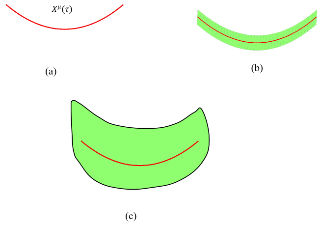
Defining as a two dimensional infinitesimal domain that satisfies the following conditions:
(i) is a part of the Minkowski spacetime.
(ii) The point of the trajectory belongs to .
(iii) is the normal vector of .
At any point along the trajectory , one can always define such an infinitesimal domain . The union of all these domains is denoted as . Then is an infinitely thin ribbon where the trajectory belongs to it, as shown in figure 1 (b).
The dimension of the infinitely thin ribbon is two. This ribbon can be extended into a two dimensional curved spacetime, as shown in figure 1 (c). We denote the metric of this curved spacetime as . As long as the ribbon is a part of the extended spacetime, the extension of the ribbon is valid. Thus, there are infinite ways to extend the ribbon .
At any point along the trajectory , the principle normal vector of the trajectory is the normal vector of the infinitesimal domain . Thus, at any point on the trajectory, is also the normal vector of the extended spacetime . In general, a curve is a geodesic on a surface if at each point of the curve, its principal normal vector is the normal vector of the surface [29]. Hence, the trajectory is a geodesic in the spacetime . Therefore, given an arbitrary trajectory in the path integral (5), one can always embed it into a curved spacetime where it becomes a geodesic. While our demonstrations are focused on the two dimensional spacetime, we believe that this conclusion holds true in higher dimensional spacetime.
References
- [1] C. Kiefer, Quantum Gravity, Oxford University Press, Oxford (2007).
- [2] C. Rovelli, Quantum Gravity, Cambridge University Press, Cambridge (2007).
- [3] H. Wang and J. Wang, Quantum cosmology of the flat universe via closed real-time path integral, Eur. Phys. J. C 82 (2022) 1172.
- [4] E. Poisson, The motion of point particles in curved space-time, Living Rev. Rel. 7 (2004) 6.
- [5] V. N. Popov, Functional integrals in quantum field theory and statistical physics, Riedel, Dordrecht (1983).
- [6] F. Mandl and G. Shaw, Quantum field theory, Wiley, Hoboken, NJ (1985).
- [7] H. Everett, “Relative State” formulation of quantum mechanics, Rev. Mod. Phys 29 (1957) 454.
- [8] R. Bousso and L. Susskind, Multiverse interpretation of quantum mechanics, Phys. Rev. D 85 (2012) 045007.
- [9] S. Ryu and T. Takayanagi, Holographic derivation of entanglement entropy from AdS/CFT, Phys. Rev. Lett. 96 (2006) 181602.
- [10] V. E. Hubeny, M. Rangamani and T. Takayanagi, A covariant holographic entanglement entropy proposal, JHEP 07 (2007) 062.
- [11] D. Baumann, Inflation, in Theoretical Advanced Study Institute in Elementary Particle Physics: Physics of the Large and the Small, World Scientific, Singapore (2011), pp. 523–686, DOI [arXiv:0907.5424].
- [12] F. W. Hehl, P. Von Der Heyde, G. D. Kerlick and J. M. Nester, General relativity with spin and torsion: foundations and prospects, Rev. Mod. Phys. 48 (1976) 393.
- [13] M. Blagojevi, Gravitation and gauge symmetries, IOP publishing, U.K. (2002).
- [14] M. Hongo, X.-G. Huang, M. Kaminski, M. Stephanov and H.-U. Yee, Relativistic spin hydrodynamics with torsion and linear response theory for spin relaxation, JHEP 11 (2021) 150.
- [15] J. M. Maldacena, The Large N limit of superconformal field theories and supergravity, Adv. Theor. Math. Phys. 2 (1998) 231.
- [16] E. Witten, Anti-de Sitter space and holography, Adv. Theor. Math. Phys. 2 253 (1998).
- [17] O. Aharony, S. S. Gubser, J. M. Maldacena, H. Ooguri and Y. Oz, Large N field theories, string theory and gravity, Phys. Rept. 323 183 (2000).
- [18] G. W. Gibbons, The Einstein action of Riemannian metrics and its relation to quantum gravity and thermodynamics, Phys. Lett. A 61 (1977) 3–5.
- [19] G. W. Gibbons, S. W. Hawking and M. J. Perry, Path integrals and the indefiniteness of the gravitational action, Nucl. Phys. B 138 (1978) 141.
- [20] K. V. Kucha, Time and interpretations of quantum gravity, in: Winnipeg, General Relativity and Relativistic Astrophysics (1991).
- [21] C. J. Isham, Canonical quantum gravity and the problem of time, arXiv:gr-qc/9210011.
- [22] S. Hashiba, Y. Yamada, Stokes phenomenon and gravitational particle production, JCAP 05 (2021) 022.
- [23] H. Wang and J. Wang, Quantum master equation for the vacuum decay dynamics, JHEP 09 (2023) 113.
- [24] H. Wang and J. Wang, Quantum geometrical current and coherence of the open gravitation system: loop quantum gravity coupled with a thermal scalar field, Phys. Scr. 98 (2023) 045303.
- [25] H.-P. Breuer and F. Petruccione, The theory of open quantum systems, Oxford University Press, New York, NY, U.S.A. (2002).
- [26] J. D. Brown, K. V. Kucha, Dust as a standard of space and time in canonical quantum gravity, Phys. Rev. D 51 (1995) 5600.
- [27] V. Husain, T. Pawlowski, Time and a physical Hamiltonian for quantum gravity, Phys. Rev. Lett. 108 (2012) 141301.
- [28] H. Maeda, Unitary evolution of the quantum universe with a Brown–Kucha dust, Class. Quantum Gravity 32 (2015) 235023.
- [29] W. H. Chen, Differential geometry, Peking university press, Beijing (2006).