Multicritical quantum sensors driven by symmetry-breaking
Abstract
Quantum criticality has been demonstrated as a useful quantum resource for parameter estimation. This includes second-order, topological and localization transitions. In all these works reported so far, gap-to-gapless transition at criticality has been identified as the ultimate resource for achieving the quantum enhanced sensing, although there are several important concepts associated with criticality, such as long-range correlation, symmetry breaking. In this work, we analytically demonstrate that symmetry-breaking can drive a quantum enhanced sensing in single- or multiparameter estimation. We show this in the well-known Kitaev model, a lattice version of the 1D -wave superconductor, which consists of a pairing term and an onsite potential term. The model is characterized by two critical lines and a multi-critical point at the intersection of these two lines. We show that Heisenberg scaling can be obtained in precision measurement of the superconducting coupling by preparing the system at or near the multicritical point despite the fact that parameter variation follows the critical lines, i.e., without an explicit requirement of gap-to-gapless transition. Quantum enhancement in such situations solely occurs due to a global symmetry-breaking by the pairing term. Extending our analysis in the realm of multiparameter estimation we show that it is possible to obtain super-Heisenberg scaling by combining the effects of symmetry-breaking and gapless-to-gapped transition.
I Introduction
The quantum Cramér-Rao bound provides the ultimate limit of precision within which an unknown parameter can be estimated in the quantum systems [1, 2, 3, 4]. The uncertainty in parameter estimation is related to a very special quantity, quantum Fisher information. The bound suggests that for the quantum systems, where is the quantum Fisher information (QFI) and is the number of repetition of the sensing protocol. Quantum systems might provide a true quantum edge over classical systems when it comes to accurately measuring an unknown variable. This is demonstrated by how the uncertainty scales with the size of the probe. Given , where is the prob size and is the associate scaling exponent, the classical probes can at-best scale linearly with system size, i.e., , which corresponds to the standard quantum limit (SQL). However, it is possible to exploit quantum phenomena, such as quantum correlation or cooperative phenomena, for achieving quantum-enhanced sensitivity, where . The so-called Heisenberg limit (HL) corresponds to [5]. Subsequently, quantum sensing [6, 2, 7] has taken the centre stage of quantum technology with several applications, and has been investigated from different points of views [5, 8, 9, 10, 11, 12].
The cooperative quantum phenomena, such as quantum phase transitions in quantum many-body (QMB) systems, has turned out to be an extremely useful quantum resource for engineering new types of quantum sensors. Quantum criticality, in its various forms, have been utilized to attain HL limit, or for even realizing beyond HL limits. This includes symmetry-breaking second-order quantum phase transitions [13, 14, 15, 16, 17, 18, 19, 20, 21, 22, 23, 24, 25, 26, 27, 28, 29, 30, 31, 32, 33, 17, 34], as well as symmetry-protected quantum phase transitions, such as localization transition [35, 36] and topological phase transition (TPT) [37, 37, 38, 39, 40, 41, 42], and non-Hermitian topological systems [43, 44, 45, 46]. There are two different key motivations for probing different kinds of quantum criticality - first, it is important to understand the basic ingredients leading to quantum-enhanced sensitivity, e.g. the role of gap closing or symmetry-breaking; secondly, there is a constant quest for identifying experimentally realizable QMB systems with super-Heisenberg scaling property characterized by large scaling exponent. It has been shown that the gap closing at criticality leads to a scaling of , where is the system size, and the critical exponent characterizing the divergence of the correlation length (localization length) near the criticality in case of the second-order quantum phase transition (localization transition). Although there are many key aspects associated with quantum criticality, such as symmetry breaking, gap closing, long-range correlation, only the gap closing has been identified as the crucial ingredient for obtaining quantum enhanced sensitivity, implying .
In this work we show that gap-to-gapless transition is always not required for quantum-enhanced sensing. Symmetry-breaking at multi-criticality can also be sufficient for it. In our knowledge such symmetry-breaking quantum advantage for quantum sensing has not been reported in literature previously. We consider well-known Kitaev model on a one-dimensional lattice with nearest neighbor hopping, onsite potential with strength and a -wave pairing term with amplitude , for demonstrating the idea analytically. The model has two critical lines at and , crossing whom one observes discrete jumps in a topological invariant. It hosts multi-critical points at the intersections of these two critical lines. The system is prepared at or near the multi-critical point. In the context of single parameter estimation we show that precision estimation of is still possible, even though then parameter variation in is restricted to follow the critical line at , where it does not encounter any gapless-to-gap transition. We show that the system still can achieve Heisenberg scaling. We expand our interest in the realm of multi-parameter sensing, where we perform simultaneous estimation of both, and . Despite the fact that parameter variations follow the gapless critical lines, super-Heisenberg scaling is observed for multi-parameter estimation. In both the cases the quantum enhanced sensing is essentially facilitated via a symmetry-breaking at , at which the system has a symmetry. This forms the central result presented in this work.
II Model
Model.– We consider the one-dimensional Kitaev lattice model [47, 48], , where
| (1) |
Here () is the creation (annihilation) operator at site of a spinless fermion, is the number of lattice sites, is an on-site potential and is the superconducting -wave pairing amplitude. This model has a rich topological phase diagram [49, 50, 51, 52], which can be characterized via a topological invariant, the winding number, . Two critical lines and set apart three topologically distinct phases: a trivial phase for with , one topologically non-trivial phase for with for , and another topologically non-trivial phase for with for . The one-dimensional Kitaev model hosts Majorana Zero Modes [53, 54] in the topological phases at both of its ends. The intersections of two critical lines marks two multicritical points in the system. The multicritical point connects two topologically non-trivial phases with a topologically trivial phase. Topological properties of a -wave spin-less superconductor have been studied from different points of views in recent years [55, 56, 57, 58, 59, 60, 51, 61]. There has been several proposals and experimental efforts for physical realization of the Kitaev -wave model [62, 56, 63, 64, 65, 66, 67, 68, 69, 70, 71, 72].
Many-body ground state.– The ground state of the Kitaev model under anti-periodic boundary conditions (ABC) is a many-particle state which is given by,
| (2) |
where and . Here with , and . The ground state is a superposition of states with multiple particle numbers but all are from even parity sector.
III Multi-Parameter sensing
Essential theory of single- and multi-parameter sensing.– Recently, sensing for more than one parameter or multi-parameter sensing has gained interest [73, 74, 75]. The parameters , of the Hamiltonian, , are encoded in the ground state. These parameters are changed, which gets reflected in the ground state. By employing the methods of the quantum Fisher information matrix (QFIM), we get a matrix given by , where and is the probe state. While considering multi-parameter sensing, the equally weighted uncertainty is given by,
| (3) |
where and is the number of repetition of the sensing protocol. The quantity is the total uncertainty for the equally weighted multi-parameter estimation. For the single-parameter estimation case, i.e., when one of the two parameters is precisely known, it is sufficient to compute the relevant diagonal element of the QFIM. Further discussion on this is presented in Appendix A.
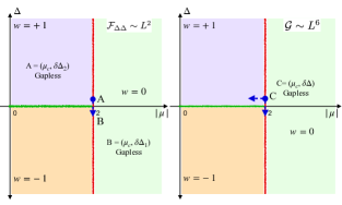
Symmetry-breaking assisted parameter estimation at multicriticality.– In absence of the pairing term, i.e., for , the system has the global symmetry as the Hamiltonian is invariant under the transformation , where is a site-independent phase. This global symmetry implies the conservation of the total fermion number. The corresponding system is gapless for parameter regime . Introduction of breaks the symmetry, and a gap opening is occurred. The phase diagram is gaped everywhere in the plane except at the critical lines at . The basic idea of the symmetry-breaking quantum enhancement of precision is the following: For parameter estimation of , assuming as a known parameter that can be precisely tuned, the many-body ground state of the system is prepared near the multi-critical point ( and ). If the system is subjected to a small variation in , it is bound to happen along the gapless critical line at . As we show below, this gives rise to Heisenberg scaling in – thanks to the symmetry-breaking. This is not the case with the parameter estimation of . It vanishes on the gapless critical line, and must involve a gap-to-gapless transition by setting non-zero. Details related to this will be furnished later. The idea, however, can be generalized for simultaneous estimation of two-parameters by combing the effects of, both, symmetry-breaking and a gap-to-gapless transition. A super-Heisenberg scaling is obtained under such scenario in . The is the main idea that we pitch in this work and is schematically presented in Fig. 1. In the following we present the results.
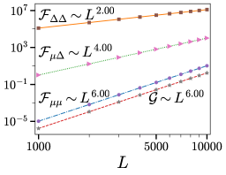
QFIM near criticality: Leading-order scaling.– We begin with summarizing the key results before we proceed to provide further details. We use fidelity based definition of for deriving the elements of QFIM for the ground state (Eq. (2)). Following expressions are obtained: , and . Unlike classical Fisher Information, which is additive, Quantum Fisher Information is super-additive. Hence, what are of prime interests are the system-size scalings of the elements of QFIM and the ultimate precision estimator . By calculating the limits of as and , we obtain closed form expressions of the leading order scalings as, , , and . Thus, we observe super-Heisenberg scaling in all quantities of our interest except for which it saturates the Heisenberg limit. These scalings of the QFIM are remarkable results establishing the importance of the multicritical point and symmetry-breaking for precision measurement of multiple parameters. This constitutes the main result of our work. The details of the derivations for obtaining the analytical expressions are presented in Appendix B.
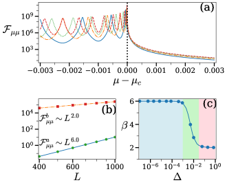
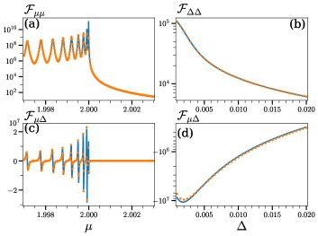
at multicriticality and beyond.– As mentioned before, . Evidently, vanishes on the critical line, . A non-vanishing value requires to prepare the system at a finite . In Fig. 2(a), we show the nature of with respect to , for a representative case, where is set at 0.001. develops a peak at .
The peak corresponds to a gap-to-gapless transition. In Fig. 2(b), we present the finite-size scaling of at and for two representative cases of with scaling exponent and with . This change in scaling exponent is gradual with change in the value of and is presented in Fig. 2(c). We observe that based on the value of , the parameter range of can be divided into three parts: small -regime with super-Heisenberg , intermediate -regime where the transitions from super-HL to SQL and large -regime where we observe SQL scaling, i.e., .
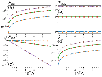
and at multicriticality and beyond.– Following expressions are obtained: and . can be computed from there-off as it is a function of , where . Validity of these expressions are further confirmed numerically. It is, however, imperative that while changing both the parameters simultaneously in an adiabatic manner, it is done in such a fashion that the parameter does not follow the critical , along which vanishes. Hence, the variation in must be guided entirely within the symmetry-broken phase with non-vanishing , and such that it encounter a gap-to-gapless transition. The parameter , however, can be navigated along the critical line, , such that it involves the symmetry-breaking transition. The combined effects of the gap-to-gapless transition and the symmetry-breaking gives rise to a super-Heisenberg scaling, as we exemplify below. It is by now obvious that the case of single parameter estimation can be done solely via symmetry-breaking by tuning precisely at and by preparing the system at or near the multicritical point.
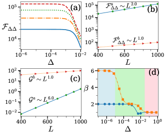
We present a set of results displaying the behavior and scaling of and with respect to the in Fig. 3(a-d). In Fig. 3(a) we present how varies with the parameter when for various system-sizes. We observe that saturates to a particular maximum value as . The quantity at becomes independent of () for very small values of , say up-to . As the value of increases, decreases gradually with increase in . It can be expected that in the thermodynamic limit. In Fig. 3(b) the finite-size scaling of is presented at for two representative cases, with super-HL scaling and with SQL scaling . We provide a similar analysis for in Fig. 3(c), where we show that has super-HL of at but a SQL scaling at a larger . In Fig. 3(d) we provide the change in the scaling exponent of and with change in . The range of values of can be divided into three subparts: small region where the scaling of saturates to HL as decreases and has a super-HL scaling of 6. In the intermediate range the scaling exponents of both of the quantities transition to SQL vale of . In the large region the scaling exponents of both the quantities saturate to 1.
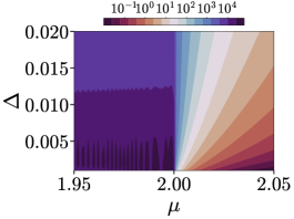
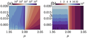
In Fig. 4, we present the variation of with respect to the parameters and for system-size . This is a representative case, and we observe similar behavior for other system-sizes as well. We observe that the value of is maximum around the critical point of . The nature of is similar to that of in the topological regime () and is similar to in the trivial phase (). The scaling exponent of saturates to 6 for smaller values of and saturates to 1 for larger values. The precision limit is inversely proportional to the quantity . Hence, total uncertainty for equally weighted multi-parameter estimation is , where is the scaling exponent of , viz. . Thus, larger the scaling of , the more precisely can one simultaneously sense and for larger system-sizes. Hence, the ground state of the Kitaev model on a one-dimensional lattice, when used as a probe, is a resource for obtaining quantum-enhanced multi-parameter sensitivity.
IV Discussions
There has been several proposals for engineering many-body quantum sensors by exploiting criticality. In all these works reported so far, gap-to-gapless transition has been identified as the key resource for achieving the quantum enhanced sensing. Other important concept associated with quantum criticality, such as symmetry-breaking, has not been shown so far to play any crucial role in parameter estimation. In this work we demonstrate for the first time that symmetry-breaking can also be a useful resource in parameter estimation. We show this by exploiting the the ground-state of the Kitaev model on a one-dimensional lattice as a candidate for a multi-parameter sensor.
The probe acting as an adiabatic sensor provides quantum-enhanced sensitivity near the multicritical point. The system admits a topological phase for and a trivial phase beyond that. The topological phase is characterized by a non-zero winding number. In addition, the point brings about a flip in the sign of the winding number when the system is in the topological phase. At the critical point of and , we obtain single-parameter scaling of the QFI-s and , whereas the multi-parameter sensitivity at this point also touches mark. Beyond this point, we do get quantum advantage in the form of super-SQL scaling for an extended region of the parameter-space. In our work, we present a phase diagram of the system and discuss how the QFIM and total uncertainty limit behave in the parameter-space of either side of the critical line.
In summary, thus, it can be said that the symmetry-breaking transition can be used as a resource, similar to gap-gapless transition, for engineering a new class of quantum sensors, as demonstrated by considering the topological Kitaev chain. It will be interesting to pursue further investigations in future, such as understanding the effects of long-range tunneling or long-range pairing on the sensing protocols proposed in this work.
Appendix A Theory of multi-parameter Sensing
Let us consider a set of parameters, , encoded in some density matrix . The precision limits of any parameter that is being sensed is given by a matrix called the Quantum Fisher Information Matrix (QFIM). The elements of the QFIM represented by is given by, , where represents the anti-commutation and the operators and are the symmetric logarithmic derivatives (SLD) with respect to and , respectively. This is given by the equation, , where, and is the partial derivative with respect to viz. . In this work, we specifically work with the many-body ground state of the Kitaev model as described in the previous section. Hence our state of interest is a pure state. For pure states, the entry reduces to . Here the state encodes the parameters . It can be seen that the diagonal elements of QFIM - reduces to the quantum fisher information for parameter .
The parameters , of the hamiltonian in Eq. (II) are encoded in the ground state. The adiabatic changes in these parameters gets reflected in the ground state. By employing the methods of the QFIM, we get a matrix , given by
| (4) |
The precision limit of a multi-parameter estimation is quantified using the covariance matrix, . This is given by
| (5) |
The QFIM is related to the covariance matrix and obeys following Cramér-Rao inequality:
| (6) |
Taking trace on both sides of the matrix inequality one obtains the scalar inequality,
| (7) |
where we define,
| (8) |
The quantity is the total uncertainty for the equally weighted multi-parameter estimation and is the number of repetition of the sensing protocol. For single-parameter estimation, where both parameters are sensed individually and independently, this precision bound reduces to,
| (9) |
Note that the off-diagonal terms are symmetric under interchange of and , i.e., . This implies that right-hand side quantity in Eq. (7) is smaller than that in Eq. (9), and hence thereby making the Eq. (7) a tighter bound than the Eq. (9). Thus, we observe that multi-parameter estimation admits same uncertainty as separate single-parameter estimations, if and only if the parameters under study are uncorrelated.
Appendix B Derivation of for ABC
The elements of QFIM for a pure state are given by,
| (10) |
For the Kitaev model the ground state is of the form [48] :
| (11) |
where stands for the momentum states, , for . For brevity, we mark via in the product above and Furthermore,
| (12) |
Here , and . Using the form,
| (13) |
| (14) |
Using this form, we arrive at the final expression:
| (15) |
We note that using . Thus, we get:
| (16) |
We find that:
| (17) |
Subsequenty, we get,
| (18) |
where and sum is over the values .
Let’s find out the scaling exponents, when we set both and . We have
| (19) |
Now, as we can see the numerator tends to zero. Therefore, largest contribution of this sum comes from the terms where the denominator also tends to zero, i.e., . This is achieved by the last term in the sum, which is given by setting and therefore . We thus get,
| (20) |
In the limit of large , we get
| (21) |
Thus, we have for and . Using similar arguments it can be easily shown that , when and .
For in the limit and , we have
| (22) |
We observe that the larger values of dominate this sum. By considering the contributions to the sum in descending order of the , one finds
| (23) |
Here, we terminate the series at some . Now we note that the Riemann zeta function at is given by
| (24) |
For very large and consequently large , we can approximate the sum in bracket of (23) with (24). We thus get,
| (25) |
Hence, we have for and . Following a similar line of reasoning as Eq.(20), we get
| (26) |
Thus, we have for and . Now, for the case of , it can be shown that
| (27) |
Thus, we have for and . In summary, one obtains,
| (28) |
In Fig. B.4 we present (a) and for system-size . We observe a similar nature for other system-sizes as well. Figure B.4 quite clearly shows the transition from topological to trivial phase at . We see in Fig. B.4(a) that the system achieves its maximum at the point . The quantity gradually decreases as we move further into the trivial phase. Due to the apparent fluctuations of in the topological phase of the finite-sized systems, particularly in smaller systems, numerical calculations were not pushed in the smaller regime. We, however, performed the scaling analysis in the trivial phase away from the critical line. In Fig. B.4(b), we present the component of QFIM. The figure clearly shows that this quantity increases as we move nearer to line, across which the system the topological invariant undergoes a discrete jump, i.e., a flip in sign of the winding number, given .
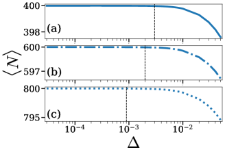
In Fig. B.5, we present the average particle number of the probe state, i.e., the ground state of the Kitaev model in one dimension for . As seen from the Hamiltonian of the Kitaev model, the -wave superconductivity term with coupling makes the system particle-number non-conserving. This means that when is set to a non-zero value, the ground state wave-function becomes a superposition of various particle-number sector. When is set to zero, we note two things: the states with fixed momentum become eigenstates of the Hamiltonian and the value of determines the fixed particle-number sector to which the ground state belongs to. We note that at limit, half of the single-particle states have negative eigenenergies. The many-body ground state of the model is constructed by filling the negative energy states via fermions. Since there is a negative sign with in the Hamiltonian, more single-particle eigenstates with negative energies becomes available with increasing . Thus, occupation number of the ground state increases gradually with increasing . On introducing a non-zero , the ground state no longer has a fixed number of particles, rather it is a superposition of many fixed particle-number states. We observe that at very small values of , the ground state has the fully-filled state with almost unit probability because of a small and a very large . As the value of increases, it becomes energetically more costly to fill up particles than that for smaller . Due to this, the average particle-number decreases with increase of . Hence, physically it turns out that at the gapless multicritical point ( and ), the system is in a trivial band-insulating phase, as all available energy states are filled-up by the fermions. A sufficiently small value of the symmetry-breaking term , i.e., , ensures the system’s transition to a critical -wave superconducting phase. This, in turn, facilitates the quantum enhanced sensing despite the fact that adiabatic variation of the parameter, , follows the gapless line throughout.
References
- Braunstein and Caves [1994] S. L. Braunstein and C. M. Caves, Statistical distance and the geometry of quantum states, Phys. Rev. Lett. 72, 3439 (1994).
- Degen et al. [2017] C. L. Degen, F. Reinhard, and P. Cappellaro, Quantum sensing, Rev. Mod. Phys. 89, 035002 (2017).
- Cramér [1946] H. Cramér, Mathematical Methods of Statistics (PMS-9), Volume 9 (Princeton University Press, Princeton, 1946).
- Helstrom [1969] C. W. Helstrom, Quantum detection and estimation theory, Journal of Statistical Physics 1, 231 (1969).
- Giovannetti et al. [2004] V. Giovannetti, S. Lloyd, and L. Maccone, Quantum-enhanced measurements: beating the standard quantum limit, Science 306, 1330 (2004).
- Giovannetti et al. [2011] V. Giovannetti, S. Lloyd, and L. Maccone, Advances in quantum metrology, Nature photonics 5, 222 (2011).
- Shi et al. [2024] H.-L. Shi, X.-W. Guan, and J. Yang, Universal shot-noise limit for quantum metrology with local hamiltonians, Phys. Rev. Lett. 132, 100803 (2024).
- Giovannetti et al. [2006] V. Giovannetti, S. Lloyd, and L. Maccone, Quantum metrology, Phys. Rev. Lett. 96, 010401 (2006).
- Manshouri et al. [2024] H. Manshouri, M. Zarei, M. Abdi, S. Bose, and A. Bayat, Quantum enhanced sensitivity through many-body bloch oscillations, arXiv preprint arXiv:2406.13921 (2024).
- Mukhopadhyay and Bayat [2023] C. Mukhopadhyay and A. Bayat, Modular many-body quantum sensors, arXiv preprint arXiv:2311.18319 (2023).
- Bhattacharyya et al. [2024] A. Bhattacharyya, D. Saha, and U. Sen, Even-body interactions favour asymmetry as a resource in metrological precision, arXiv preprint arXiv:2401.06729 (2024).
- Yousefjani et al. [2024a] R. Yousefjani, K. Sacha, and A. Bayat, Discrete time crystal phase as a resource for quantum enhanced sensing, arXiv preprint arXiv:2405.00328 (2024a).
- Zanardi and Paunković [2006] P. Zanardi and N. Paunković, Ground state overlap and quantum phase transitions, Phys. Rev. E 74, 031123 (2006).
- Gu et al. [2008] S.-J. Gu, H.-M. Kwok, W.-Q. Ning, and H.-Q. Lin, Fidelity susceptibility, scaling, and universality in quantum critical phenomena, Phys. Rev. B 77, 245109 (2008).
- Zanardi et al. [2008] P. Zanardi, M. G. A. Paris, and L. Campos Venuti, Quantum criticality as a resource for quantum estimation, Phys. Rev. A 78, 042105 (2008).
- Invernizzi et al. [2008] C. Invernizzi, M. Korbman, L. Campos Venuti, and M. G. A. Paris, Optimal quantum estimation in spin systems at criticality, Phys. Rev. A 78, 042106 (2008).
- GU [2010] S.-J. GU, Fidelity approach to quantum phase transitions, International Journal of Modern Physics B 24, 4371 (2010), https://doi.org/10.1142/S0217979210056335 .
- Gammelmark and Mølmer [2011] S. Gammelmark and K. Mølmer, Phase transitions and heisenberg limited metrology in an ising chain interacting with a single-mode cavity field, New Journal of Physics 13, 053035 (2011).
- Skotiniotis et al. [2015] M. Skotiniotis, P. Sekatski, and W. Dür, Quantum metrology for the ising hamiltonian with transverse magnetic field, New Journal of Physics 17, 073032 (2015).
- Rams et al. [2018] M. M. Rams, P. Sierant, O. Dutta, P. Horodecki, and J. Zakrzewski, At the limits of criticality-based quantum metrology: Apparent super-heisenberg scaling revisited, Phys. Rev. X 8, 021022 (2018).
- Wei [2019] B.-B. Wei, Fidelity susceptibility in one-dimensional disordered lattice models, Phys. Rev. A 99, 042117 (2019).
- Chu et al. [2021] Y. Chu, S. Zhang, B. Yu, and J. Cai, Dynamic framework for criticality-enhanced quantum sensing, Phys. Rev. Lett. 126, 010502 (2021).
- Huggins et al. [2021] W. J. Huggins, J. R. McClean, N. C. Rubin, Z. Jiang, N. Wiebe, K. B. Whaley, and R. Babbush, Efficient and noise resilient measurements for quantum chemistry on near-term quantum computers, npj Quantum Information 7, 23 (2021).
- Mirkhalaf et al. [2021] S. S. Mirkhalaf, D. Benedicto Orenes, M. W. Mitchell, and E. Witkowska, Criticality-enhanced quantum sensing in ferromagnetic bose-einstein condensates: Role of readout measurement and detection noise, Physical Review A 103, 023317 (2021).
- Di Candia et al. [2023] R. Di Candia, F. Minganti, K. Petrovnin, G. Paraoanu, and S. Felicetti, Critical parametric quantum sensing, npj Quantum Information 9, 23 (2023).
- Salvia et al. [2023] R. Salvia, M. Mehboudi, and M. Perarnau-Llobet, Critical quantum metrology assisted by real-time feedback control, Phys. Rev. Lett. 130, 240803 (2023).
- Mishra and Bayat [2021] U. Mishra and A. Bayat, Driving enhanced quantum sensing in partially accessible many-body systems, Phys. Rev. Lett. 127, 080504 (2021).
- Montenegro et al. [2021] V. Montenegro, U. Mishra, and A. Bayat, Global sensing and its impact for quantum many-body probes with criticality, Phys. Rev. Lett. 126, 200501 (2021).
- Montenegro et al. [2022] V. Montenegro, G. S. Jones, S. Bose, and A. Bayat, Sequential measurements for quantum-enhanced magnetometry in spin chain probes, Phys. Rev. Lett. 129, 120503 (2022).
- Monika et al. [2023] Monika, L. G. C. Lakkaraju, S. Ghosh, and A. S. De, Better sensing with variable-range interactions (2023), arXiv:2307.06901 [quant-ph] .
- Singh et al. [2024] S. Singh, L. G. C. Lakkaraju, S. Ghosh, and A. S. De, Dimensional gain in sensing through higher-dimensional quantum spin chain (2024), arXiv:2401.14853 [quant-ph] .
- Dooley et al. [2023] S. Dooley, S. Pappalardi, and J. Goold, Entanglement enhanced metrology with quantum many-body scars, Phys. Rev. B 107, 035123 (2023).
- Montenegro et al. [2023] V. Montenegro, M. G. Genoni, A. Bayat, and M. G. A. Paris, Quantum metrology with boundary time crystals, Communications Physics 6, 304 (2023).
- Pezzè et al. [2019] L. Pezzè, A. Trenkwalder, and M. Fattori, Adiabatic sensing enhanced by quantum criticality, arXiv preprint arXiv:1906.01447 (2019).
- He et al. [2023] X. He, R. Yousefjani, and A. Bayat, Stark localization as a resource for weak-field sensing with super-heisenberg precision, Phys. Rev. Lett. 131, 010801 (2023).
- Sahoo et al. [2024] A. Sahoo, U. Mishra, and D. Rakshit, Localization-driven quantum sensing, Phys. Rev. A 109, L030601 (2024).
- Zhang et al. [2018] Y.-R. Zhang, Y. Zeng, H. Fan, J. Q. You, and F. Nori, Characterization of topological states via dual multipartite entanglement, Phys. Rev. Lett. 120, 250501 (2018).
- Lambert and Sørensen [2020] J. Lambert and E. S. Sørensen, Revealing divergent length scales using quantum fisher information in the kitaev honeycomb model, Phys. Rev. B 102, 224401 (2020).
- Yin et al. [2019] S. Yin, J. Song, Y. Zhang, and S. Liu, Quantum fisher information in quantum critical systems with topological characterization, Phys. Rev. B 100, 184417 (2019).
- Zhang et al. [2022] Y.-R. Zhang, Y. Zeng, T. Liu, H. Fan, J. Q. You, and F. Nori, Multipartite entanglement of the topologically ordered state in a perturbed toric code, Phys. Rev. Res. 4, 023144 (2022).
- Yang et al. [2022] J. Yang, S. Pang, A. del Campo, and A. N. Jordan, Super-heisenberg scaling in hamiltonian parameter estimation in the long-range kitaev chain, Phys. Rev. Res. 4, 013133 (2022).
- Sarkar et al. [2022] S. Sarkar, C. Mukhopadhyay, A. Alase, and A. Bayat, Free-fermionic topological quantum sensors, Phys. Rev. Lett. 129, 090503 (2022).
- Wiersig [2014] J. Wiersig, Enhancing the sensitivity of frequency and energy splitting detection by using exceptional points: Application to microcavity sensors for single-particle detection, Phys. Rev. Lett. 112, 203901 (2014).
- Schomerus [2020] H. Schomerus, Nonreciprocal response theory of non-hermitian mechanical metamaterials: Response phase transition from the skin effect of zero modes, Phys. Rev. Res. 2, 013058 (2020).
- Budich and Bergholtz [2020] J. C. Budich and E. J. Bergholtz, Non-hermitian topological sensors, Phys. Rev. Lett. 125, 180403 (2020).
- Koch and Budich [2022] F. Koch and J. C. Budich, Quantum non-hermitian topological sensors, Phys. Rev. Res. 4, 013113 (2022).
- Kitaev [2001] A. Y. Kitaev, Unpaired majorana fermions in quantum wires, Physics-Uspekhi 44, 131 (2001).
- Mbeng et al. [2024] G. B. Mbeng, A. Russomanno, and G. E. Santoro, The quantum Ising chain for beginners, SciPost Phys. Lect. Notes , 82 (2024).
- Leijnse and Flensberg [2012] M. Leijnse and K. Flensberg, Introduction to topological superconductivity and majorana fermions, Semiconductor Science and Technology 27, 124003 (2012).
- Elliott and Franz [2015] S. R. Elliott and M. Franz, Colloquium: Majorana fermions in nuclear, particle, and solid-state physics, Rev. Mod. Phys. 87, 137 (2015).
- Maity et al. [2019] S. Maity, U. Bhattacharya, and A. K. Dutta, One-dimensional quantum many body systems with long-range interactions, Journal of Physics A: Mathematical and Theoretical 53 (2019).
- Pezzè et al. [2017] L. Pezzè, M. Gabbrielli, L. Lepori, and A. Smerzi, Multipartite entanglement in topological quantum phases, Phys. Rev. Lett. 119, 250401 (2017).
- Hasan and Kane [2010] M. Z. Hasan and C. L. Kane, Colloquium: Topological insulators, Rev. Mod. Phys. 82, 3045 (2010).
- Asbóth et al. [2016] J. K. Asbóth, L. Oroszlány, and A. Pályi, A short course on topological insulators, Lecture notes in physics 919, 166 (2016).
- Fulga et al. [2011] I. C. Fulga, F. Hassler, A. R. Akhmerov, and C. W. J. Beenakker, Scattering formula for the topological quantum number of a disordered multimode wire, Phys. Rev. B 83, 155429 (2011).
- Sau and Sarma [2012] J. D. Sau and S. D. Sarma, Realizing a robust practical majorana chain in a quantum-dot-superconductor linear array, Nature Communications 3, 964 (2012).
- Lutchyn and Fisher [2011] R. M. Lutchyn and M. P. A. Fisher, Interacting topological phases in multiband nanowires, Phys. Rev. B 84, 214528 (2011).
- DeGottardi et al. [2011] W. DeGottardi, D. Sen, and S. Vishveshwara, Topological phases, majorana modes and quench dynamics in a spin ladder system, New Journal of Physics 13, 065028 (2011).
- DeGottardi et al. [2013] W. DeGottardi, D. Sen, and S. Vishveshwara, Majorana fermions in superconducting 1d systems having periodic, quasiperiodic, and disordered potentials, Phys. Rev. Lett. 110, 146404 (2013).
- Thakurathi et al. [2013] M. Thakurathi, A. A. Patel, D. Sen, and A. Dutta, Floquet generation of majorana end modes and topological invariants, Phys. Rev. B 88, 155133 (2013).
- Fraxanet et al. [2021] J. Fraxanet, U. Bhattacharya, T. Grass, D. Rakshit, M. Lewenstein, and A. Dauphin, Topological properties of the long-range kitaev chain with aubry-andré-harper modulation, Phys. Rev. Res. 3, 013148 (2021).
- Fu and Kane [2008] L. Fu and C. L. Kane, Superconducting proximity effect and majorana fermions at the surface of a topological insulator, Phys. Rev. Lett. 100, 096407 (2008).
- Mourik et al. [2012] V. Mourik, K. Zuo, S. M. Frolov, S. Plissard, E. P. Bakkers, and L. P. Kouwenhoven, Signatures of majorana fermions in hybrid superconductor-semiconductor nanowire devices, Science 336, 1003 (2012).
- Deng et al. [2012] M. T. Deng, C. L. Yu, G. Y. Huang, M. Larsson, P. Caroff, and H. Q. Xu, Anomalous zero-bias conductance peak in a nb–insb nanowire–nb hybrid device, Nano Letters 12, 6414 (2012).
- Das et al. [2012] A. Das, Y. Ronen, Y. Most, Y. Oreg, M. Heiblum, and H. Shtrikman, Zero-bias peaks and splitting in an al–inas nanowire topological superconductor as a signature of majorana fermions, Nature Physics 8, 887 (2012).
- Fulga et al. [2013] I. C. Fulga, A. Haim, A. R. Akhmerov, and Y. Oreg, Adaptive tuning of majorana fermions in a quantum dot chain, New Journal of Physics 15, 045020 (2013).
- Nadj-Perge et al. [2014] S. Nadj-Perge, I. K. Drozdov, J. Li, H. Chen, S. Jeon, J. Seo, A. H. MacDonald, B. A. Bernevig, and A. Yazdani, Observation of majorana fermions in ferromagnetic atomic chains on a superconductor, Science 346, 602 (2014), https://www.science.org/doi/pdf/10.1126/science.1259327 .
- Xu et al. [2016] J.-S. Xu, K. Sun, Y.-J. Han, C.-F. Li, J. K. Pachos, and G.-C. Guo, Simulating the exchange of majorana zero modes with a photonic system, Nature Communications 7, 13194 (2016).
- Xing et al. [2018] Y. Xing, L. Qi, J. Cao, D.-Y. Wang, C.-H. Bai, W.-X. Cui, H.-F. Wang, A.-D. Zhu, and S. Zhang, Controllable photonic and phononic edge localization via optomechanically induced kitaev phase, Opt. Express 26, 16250 (2018).
- Dvir et al. [2023] T. Dvir, G. Wang, N. van Loo, C.-X. Liu, G. P. Mazur, A. Bordin, S. L. D. ten Haaf, J.-Y. Wang, D. van Driel, F. Zatelli, X. Li, F. K. Malinowski, S. Gazibegovic, G. Badawy, E. P. A. M. Bakkers, M. Wimmer, and L. P. Kouwenhoven, Realization of a minimal kitaev chain in coupled quantum dots, Nature 614, 445 (2023).
- Liu et al. [2022] C.-X. Liu, G. Wang, T. Dvir, and M. Wimmer, Tunable superconducting coupling of quantum dots via andreev bound states in semiconductor-superconductor nanowires, Phys. Rev. Lett. 129, 267701 (2022).
- Zhang et al. [2023] Y. Zhang, Y.-Q. Ge, and Y. xi Liu, Simulation of kitaev model using one-dimensional chain of superconducting qubits and environmental effect on topological states (2023), arXiv:2302.03834 [quant-ph] .
- Fresco et al. [2022] G. D. Fresco, B. Spagnolo, D. Valenti, and A. Carollo, Multiparameter quantum critical metrology, SciPost Phys. 13, 077 (2022).
- Mihailescu et al. [2024] G. Mihailescu, A. Bayat, S. Campbell, and A. K. Mitchell, Multiparameter critical quantum metrology with impurity probes, Quantum Science and Technology 9, 035033 (2024).
- Yousefjani et al. [2024b] R. Yousefjani, X. He, A. Carollo, and A. Bayat, Nonlinearity-enhanced quantum sensing in stark probes, arXiv preprint arXiv:2404.10382 (2024b).