System-$1.x$: Learning to Balance Fast and Slow Planning with Language Models

Abstract

Language models can be used to solve long-horizon planning problems in two distinct modes. In a fast ‘System-$1$’ mode, models directly generate plans without any explicit search or backtracking, and in a slow ‘System-$2$’ mode, they plan step-by-step by explicitly searching over possible actions. While System-$2$ planning is typically more effective, it is also more computationally expensive, often making it infeasible for long plans or large action spaces. Moreover, isolated System-$1$ or System-$2$ planning ignores the user’s end goals and constraints (e.g., token budget), failing to provide ways for the user to control their behavior. To this end, we propose the System-$1.x$ Planner, a controllable planning framework with language models that is capable of generating hybrid plans and balancing between the two planning modes based on the difficulty of the problem at hand. System-$1.x$ consists of (i) a controller, (ii) a System-$1$ Planner, and (iii) a System-$2$ Planner. Based on a user-specified hybridization factor $x$ governing the degree to which the system uses System-$1$ vs. System-$2$, the controller decomposes a planning problem into sub-goals, and classifies them as easy or hard to be solved by either System-$1$ or System-$2$, respectively. We fine-tune all three components on top of a single base LLM, requiring only search traces as supervision. Experiments with two diverse planning tasks – Maze Navigation and Blocksworld – show that our System-$1.x$ Planner outperforms a System-$1$ Planner, a System-$2$ Planner trained to approximate A^∗ search, and also a symbolic planner (A^∗ search), given an exploration budget. We also demonstrate the following key properties of our planner: (1) controllability: by adjusting the hybridization factor $x$ (e.g., System-$1.75$ vs. System-$1.5$) we can perform more (or less) search, improving performance, (2) flexibility: by building a neuro-symbolic variant composed of a neural System-$1$ planner and a symbolic System-$2$ planner, we can take advantage of existing symbolic methods, and (3) generalizability: by learning from different search algorithms (BFS, DFS, A^∗), we show that our method is robust to the choice of search algorithm used for training.

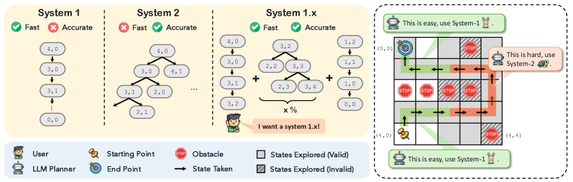
Figure 1: Comparative overview of a System-$1$ Planner, a System-$2$ Planner, and our hybrid and controllable System-$1.x$ Planner. Given a Maze Navigation task, a System-$1$ Planner directly generates a plan as a sequence of steps without search, thus making it fast but inaccurate. A System-$2$ Planner performs search before generating a plan and hence is more accurate but much slower. Our System-$1.x$ Planner generates hybrid plans, where the level of hybridization is controlled by a user-defined hyperparameter. Hybrid plans balance System-$1$ sub-plans for easier sub-goals and System-$2$ sub-plans for harder ones, making System-$1.x$ fast, accurate, and controllable.

1 Introduction

A key feature of intelligence – both human and artificial – is the ability to plan. Indeed, planning has been a major topic of research in AI for most of its history (Russell and Norvig, 2016), with applications ranging from navigation and robotics to manufacturing and story-telling. These days, auto-regressive Large Language Models (LLMs) are increasingly used for various long-horizon planning and reasoning tasks (Bubeck et al., 2023; Wei et al., 2022; Yao et al., 2024). Despite some initial promise, recent careful investigations have highlighted LLMs’ shortcomings on classical planning tasks (Pallagani et al., 2023; Valmeekam et al., 2023, 2024; Momennejad et al., 2024). Supervising models with correct plans has also led to limited success, especially for out-of-distribution generalization (Dziri et al., 2023). Fundamentally, this issue is attributed to a lack of explicit search, backtracking, or learning from mistakes (Kambhampati et al., 2024; Bachmann and Nagarajan, 2024; Gandhi et al., 2024), all of which are essential components of standard planning systems. In other words, LLMs directly generating plans generally resemble humans’ fast ‘System-$1$’ decision-making process (Kahneman, 2011), characterized by quick, intuitive judgments rather than slow, deliberate planning (Kambhampati et al., 2024).

As potential remedies, slow ‘System-$2$’-inspired LLM planning approaches have emerged that either (1) augment LLMs during inference with symbolic search algorithms (Yao et al., 2024; Sel et al., 2023; Ahn et al., 2022) or (2) directly teach LLMs to carry out search themselves (Gandhi et al., 2024; Lehnert et al., 2024). While the former approach of using external search tools can enhance test-time performance, the latter approach – training models to search – has the advantage of resulting in a single unified search model and also discovering better and more efficient search strategies (Gandhi et al., 2024). However, such training-time approaches also face challenges due to high computational demands and potential infeasiblity. For instance, one such recently proposed (trained) System-$2$ method, Searchformer, uses token sequences that verbalize entire search trajectories (Lehnert et al., 2024). Consequently, during inference, based on the action space and the plan length, these models explore a large number of states, resulting in an increased number of generated tokens. The cost of exploration is further exacerbated by the fact that Transformers (Vaswani et al., 2017) typically exhibit quadratic complexity w.r.t. the sequence length. Thus, as sequence length increases, the computational complexity grows, significantly impacting memory usage and speed, rendering many long-horizon tasks infeasible due to token limits. A more promising alternative would thus be to avoid incurring a high cost on all samples and steps by training a planner with a smarter, more balanced allocation of compute, i.e. one that uses System-$1$ for easier (sub-)problems while reserving the more expensive System-$2$ for harder (sub-)problems based on the budget.

To this end, we propose the System-$1.x$ Planner, drawing inspiration from the Dual-Process Theory (Wason and Evans, 1974; Kahneman, 2011) that argues for the co-existence of fast and slow planning in humans. The fast system relies on expertise and quick judgments that are learned from experience; it can be cheaply and quickly applied either instinctively (e.g., withdrawing one’s hand from a hot object) or in areas where an individual has acquired expertise (e.g., avoiding an unexpected obstacle when driving). The slow system is more costly, involving sequential processing and relying on working memory to formulate a more deliberate plan; it includes the consideration of hypothetical alternatives (Evans, 2003). Crucially, people can switch between these two modes as determined by the task at hand (Kahneman, 2011). For example, imagine someone is taking a detour on their usual route home. While on the detour, they might require System-$2$ planning to handle navigation in an unfamiliar area but can switch to System-$1$’s “autopilot” as soon as they are back on their familiar route. Based on this distinction, we develop the System-$1.x$ Planner, a controllable framework for long-horizon planning with LLMs that is capable of generating hybrid plans interleaved with System-$1$ and System-$2$ sub-plans. System-$1.x$ offers a promising middle ground between a fast but inaccurate System-$1$ Planner, used for easy problems, and an accurate but slow System-$2$ Planner, used for hard problems (see Fig. 1 for an overview).

At its core, System-$1.x$ is composed of three trained components: (1) a controller that decomposes a planning problem into easier and harder sub-goals, (2) a System-$1$ Planner that solves the easier sub-goals without any explicit search or exploration, and (3) a System-$2$ Planner that solves the harder sub-goals by deliberately searching over possible actions. One of the primary strengths of System-$1.x$ is its train-time controllability – based on a user-specified hyperparameter $x\in[0,1]$, we train a controller that ultimately governs the degree of hybridization between the System-$1$ and $2$ planners. Moreover, it also offers test-time controllability, by which an already trained controller can be adjusted towards solving more or fewer problems using System-$2$, providing another level of inference-time compute. Importantly, all three components are implemented by the same fine-tuned LLM, using only search traces supervision. System-$1.x$ is thus a fully (LLM-based) neural planner that does not rely on external solvers or verifiers and requires only one base LLM. By not relying on external tools, our method has an advantage over inference-time methods that rely on symbolic planners, as external tools may not exist for certain domains, making data-driven approaches like System-$1.x$ self-contained and easier to apply to new domains and to scale up. At the same time, System-$1.x$ can also be seamlessly converted into a neuro-symbolic planner by replacing the System-$2$ Planner with a symbolic solver (e.g., A^∗), allowing us to integrate powerful symbolic tools when they are available.

We experiment with two diverse planning problems: Maze Navigation and Blocksworld. We demonstrate that our System-$1.x$ Planner matches and generally outperforms a System-$1$ Planner, a System-$2$ Planner, and a System-$1.x$ variant (without sub-goal decomposition) at all budgets by up to $33\%$ absolute accuracy. We also report similar findings with our neuro-symbolic System-$1.x$, that in fact typically outperforms symbolic search, beating A^∗ by up to 39% at a fixed budget and matching it at maximum budget. Next, we show the controllability of our framework by training a System-$1.75$ Planner that, compared to a System-$1.5$ Planner, trades off efficiency for greater accuracy. This trend can be continued to recover the full System-$2$ performance. System-$1.x$ also generalizes to different search algorithms (BFS, DFS, and A^∗) and exhibits exploration behavior that closely resembles the corresponding algorithm it is trained on. Overall, the System-$1.x$ Planner introduces a novel way of applying LLMs to controllable and hybrid planning, optimizing for both accuracy and efficiency. This, in turn, allows System-$1.x$ to outperform both System-$1$ and System-$2$ at a fixed budget. By intelligently allocating more resources to harder sub-goals, System-$1.x$ is able to save its System-$2$ budget for cases where it is necessary.

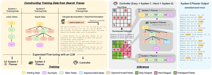
Figure 2: Overview of our System-$1.x$ Planner. Left: The process for training data construction. We generate three kinds of data to fine-tune our three components: (1) System-$1$ data (linear chains), (2) System-$2$ data (search trees), and (3) controller data (consisting of sub-goals and easy/hard annotations) conditioned on a user-specified hybridization factor $x$. Right: During inference, the controller generates the sub-goals and predicts whether each is easy or hard. Then, it invokes System-$1$ and System-$2$ for easy and hard sub-goals respectively to construct the final plan.

2 System-$1.x$: Controllable and Hybrid Planning with LLMs

We start with the requisite background on planning problems and our setup (Section 2.1), followed by an overview and a detailed description of our method System-$1.x$ Planner in Section 2.2 and Section 2.3, respectively.

2.1 Background and Problem Setup

A planning problem can be modeled as a Markov Decision Process $\mathcal{M}=(\mathcal{S},\mathcal{A},\mathcal{T},\mathcal{R})$ defined with a set of states $\mathcal{S}$, a set of actions $\mathcal{A}$ on any given state, a transition function $\mathcal{T}:\mathcal{S}\times\mathcal{A}\rightarrow\mathcal{S}$ defining transitions between pairs of states based on an action, and a reward function $\mathcal{R}:\mathcal{S}\rightarrow\mathbb{R}$ assigning a reward for reaching the goal state. Given such a planning problem, a start state $s_{0}\in\mathcal{S}$ and a goal state $s_{g}\in\mathcal{S}$, the objective of classical planning is to generate a plan $\mathcal{P}=(a_{1},...,a_{n})$, as a sequence of $n$ actions $a_{i}\in\mathcal{A}$ that helps transition from the start state to the goal state. Using this notation, we define some salient concepts in a planning problem below:

• System-$1$ Planner. We use the term “System-$1$ Planner” to denote any planner that directly generates a plan as a sequence of actions without conducting any exploration or search. System-$1$ Planners are typically only model-based, trained to only output the final plan. Within the scope of this study, a System-$1$ Planner will specifically refer to a neural LLM-based planner.

• System-$2$ Planner. We use the term “System-$2$ Planner” to denote planners that do conduct search before generating a plan. Unlike model-based System-$1$ Planners, System-$2$ Planners can either be symbolic or model-based. Symbolic System-$2$ Planners are search algorithms. Ones that do not rely on heuristics to minimize the search space are called uninformed algorithms (e.g., Depth First Search or Breadth First Search), and the ones that do are called informed (e.g., Greedy Best First or A^∗). A model-based System-$2$ Planner, within the scope of this study, will specifically refer to an LLM trained to verbalize search trajectories (defined below) before generating a plan. Thus, the terms System-$1$ and System-$2$ will refer to LLM-based planners while symbolic algorithms will be addressed separately.

• Search Trajectory. Given a search algorithm, we define a search trajectory or a search trace as the step-by-step execution of the algorithm for an input problem; in the context of LLMs, this will mean a verbalized representation of a search trajectory. Trajectories consist of the final plan, all intermediate actions explored during search, their corresponding states, their validity, etc.

• Valid Plan: A plan $\mathcal{P}=(a_{1},...,a_{n})$ is considered valid if starting from the start state $s_{0}$, sequentially executing all taken actions in the plan leads to the goal state $s_{g}$, or more formally, $\mathcal{T}(\mathcal{T}(...\mathcal{T}(s_{0},a_{1})...,a_{n-1}),a_{n})=s_{g}$. Plan Validity is a metric measuring the percentage of valid plans, i.e., the accuracy of the generated plans in reaching the goal state.

• #States-Explored: Given a planning problem and a planner (System-$1$, $2$, or $1.x$), we define #States-Explored ($\mathit{SE}$, in short) as the set of all states (both valid as well as invalid) that are visited by the planner on its way to generating the plan. In the case of an LLM planner, this corresponds to the number of states that the planner needs to verbalize for exploration (see right of Fig. 2 for an example output), and thus adds to the token cost of generation. Since a System-$1$ Planner generates a plan directly without any additional explorations, it only explores the states that are part of its plan, i.e., $\mathit{SE}_{\textrm{Sys1}}\!=\!n$, where $n$ is the length of the generated plan. A System-$2$ Planner, on the other hand, will perform additional state explorations before generating a plan, resulting in $\mathit{SE}_{\textrm{Sys2}}\gg\mathit{SE}_{\textrm{Sys1}}$. Note that #States-Explored for a System-$2$ Planner will vary based on the underlying search algorithm or the LLM planner learning from that algorithm’s traces. For example, A^∗, being an informed search algorithm, will typically explore fewer states than Breadth First Search. Similarly, an LLM trained on such A^∗ traces is expected to be more efficient than the one trained on BFS’s traces. Plan Validity (i.e., plan accuracy) and #States-Explored will be our two metrics of interest, using which we will compare the performance at varying budgets of all planners (discussed in Section 4).

• Sub-goal. Finally, planning problems are typically compositional, meaning that they can be decomposed into sub-problems, which we will refer to as sub-goals. Formally, given a plan $P$ between states $s_{0}$ and $s_{g}$, a sub-goal can be characterized by a pair of states $(s_{i},s_{j})$ s.t. $i,j\in[0,g],i\leq j$, where $s_{i}$ and $s_{j}$ are intermediate states on the plan to get from $s_{0}$ to $s_{g}$.

Problem Setup.

Having defined the key terms and metrics above, we now describe the setup underlying System-$1.x$ Planner. To build a System-$1.x$ Planner, we assume access to two things: (1) a training dataset $\mathcal{D}$ of search trajectories for $N$ planning problems, and (2) a user-specified hybridization factor $x\in[0,1]$. Given a planning problem of initial state $s_{0}$, goal state $s_{g}$, and a gold plan $\mathcal{P}$, let us denote the corresponding gold search trajectory as $\mathcal{T}$, making the training dataset $\mathcal{D}=\{(s_{0}^{(i)},s_{g}^{(i)}),\mathcal{P}^{(i)},\mathcal{T}^{(i)}\}_{i=1}^{N}$. In our experiments, the gold plans and the corresponding trajectories will be obtained using a symbolic System-$2$ Planner (e.g., A^∗ search) but more generally, the source of these trajectories could be any neural or symbolic engine capable of exploration or search. The hybridization factor $x$ is a user-defined hyperparameter that will determine the balance between System-$1$ and System-$2$.

2.2 System-$1.x$ Overview

Using the setup described in Section 2.1, we develop our System-$1.x$ Planner that consists of three trained components: (i) a Controller for decomposing planning problems into sub-goals and classifying them into easy or hard sub-goals, (ii) a System-$1$ Planner for fast planning of easy sub-goals, and (iii) a System-$2$ Planner for slow planning of hard sub-goals. See Fig. 2 for an overview. We train all three components by automatically generating data from the gold search traces in a way that also respects the user’s constraints (specified in the form of the hybridization factor). In the following two subsections, we describe how we train each component and how all three join to make System-$1.x$.

2.3 Training Data Generation for System-$1.x$

System-$1$ Planner Training Data.

The training data for the System-$1$ Planner is $\mathcal{D}_{\textrm{Sys1}}\!=\!\{(s_{0}^{(i)},s_{g}^{(i)}),\mathcal{P}^{(i)}\}_{i=1}^{N}$ where the input is a natural language description of the planning problem consisting of a start state $s_{0}^{(i)}$ and a goal state $s_{g}^{(i)}$ and the output is the corresponding plan in natural language $\mathcal{P}^{(i)}$ (see Appendices C and C for examples). For the Maze domain, these gold plans are also optimal plans while for Blocksworld, they may include additional explorations, making them sub-optimal at times (though they are always valid).

System-$2$ Training Data.

Similar to System-$1$, the input to a System-$2$ Planner is also a natural language description of the planning problem. However, the target output of the System-$2$ Planner is a verbalized search trajectory $\mathcal{T}^{(i)}$ as described in Section 2.1 (refer to Appendices C and C for examples). This yields a training dataset of $\mathcal{D}_{\textrm{Sys2}}\!=\!\{(s_{0}^{(i)},s_{g}^{(i)}),\mathcal{T}^{(i)}\}_{i=1}^{N}$.

Controller Training Data.

Recall that the System-$1.x$ Planner is designed to minimize state explorations by only performing System-$2$ planning as needed, i.e., saving states by employing System-1 for easier sub-goals and reserving search with System-2 for harder sub-goals. Hence, the role of the controller is two-fold: (i) decomposing a problem into sub-goals characterized by a start and end state $(s_{i},s_{j})$, and (ii) classifying those sub-goals as easy or hard so that System-2 can be invoked only for the hard sub-goals. However, most planning domains lack gold annotations of sub-goal decompositions and their easy and hard classifications. Therefore, we propose an automatic data generation process for training our controller, as described below and more formally in Algorithm 1. The inputs to preparing the controller data are (1) the gold plans $\{\mathcal{P}^{(i)}\}_{i=1}^{N}$ that will be decomposed into sub-goals, (2) the user-defined hybridization factor $x$, and (3) a hardness function $h(\cdot,\cdot)$ for (sub-)goals.

Algorithm 1 Training Data Generation for System-$1.x$ Controller

Input: System-$1$ Training Data $\mathcal{D}_{\textrm{Sys1}}=\{(s_{0}^{(i)},s_{g}^{(i)}),\mathcal{P}^{(i)}\}_{i=1}^{N}$, Hybridization Factor $x\in[0,1]$, Hardness Function $h(\cdot,\cdot)$

Output: Training Data $\mathcal{D}_{c}$ for System-$1.x$ Controller

${\tt sort}$$(\mathcal{D}_{\textrm{Sys1}},{\tt{key}}\!=\!h(s_{0},s_{g}))$ // Ranking data points in increasing order of hardness

$\mathcal{D}_{c}\leftarrow\{\}$ data point $((s_{0}^{(i)},s_{g}^{(i)}),\mathcal{P}^{(i)})\in\mathcal{D}_{\textrm{Sys1}}$ $i<(1-x)\times N$

// For the first ($1-x$)% of instances (easiest), solve them directly using System-$1$ planner

$y^{(i)}\leftarrow\{(s_{0}^{(i)},s_{g}^{(i)}),\textrm{``Sys1''}\}$ :

// For the remaining x% hardest instances, find the best decomposition into three sub-goals such that the middle sub-goal $(s_{j},s_{k})$ is solved using System-$2$ and has a length of x% of the total plan length

$(j,k)=\mathrm{argmin}_{u,v\in[0,g],u\leq v}(h(s_{0}^{(i)},s_{u})-h(s_{u},s_{v})+h(s_{v},s_{g}^{(i)}))\text{ s.t. }|v-u|=x\times n$

$y^{(i)}\leftarrow\{(s_{0}^{(i)},s_{j}),\textrm{``Sys1''}\}$

$y^{(i)}\leftarrow y^{(i)}+\{(s_{j},s_{k}),\textrm{``Sys2''}\}$

$y^{(i)}\leftarrow y^{(i)}+\{(s_{k},s_{g}^{(i)}),\textrm{``Sys1''}\}$

$\mathcal{D}_{c}\leftarrow\mathcal{D}_{c}+\{(s_{0}^{(i)},s_{g}^{(i)}),y^{(i)}\}$

$\mathcal{D}_{c}$

• Step 1: Defining and Ranking using a Hardness Function. A hardness function $h(s_{i},s_{j})$ takes a start state $s_{i}$ and a goal state $s_{j}$ as input, and returns a scalar value estimating the hardness of the goal or the sub-goal. An example of a hardness function for a Maze Navigation task is the number of obstacles in a sub-maze, where a higher value indicates greater difficulty. Sections Section 3.4, and Section 4.3 more concretely describe and compare these hardness functions for different tasks, respectively. Generally, hardness functions can be constructed for most planning domains where heuristic searches like A^∗ are frequently applied. Using this hardness function between the start and the goal state $h(s_{0},s_{g})$, we generate a rank ordering of the training examples.

• Step 2: Annotating Easy Instances as System-$1$-only. Intuitively, some planning problems in the train set can be solved successfully via only a System-$1$ Planner. For such instances, no further decomposition is needed. These correspond to the first $(1-x)\times N$ easiest samples with the least $h(\cdot,\cdot)$. Note that this is a definition of hardness, and what is considered as easy is determined by the hybridization factor $x$. For example, when $x=0.0$, all samples will be annotated as easy, making System-$1.x$ the same as System-$1$.

• Step 3: Annotating Hard Instances as Hybrid System-$1$ + System-$2$. For the remaining $x\times N$ (hard) samples, we assume that they can be decomposed into sub-goals, each of which can be assigned to either System-$1$ or System-$2$. However, to ensure overall task success, the decompositions should neither be too coarse, i.e., requiring further decompositions, nor too fine-grained, making them susceptible to decomposition errors (Prasad et al., 2024). Hence, we adopt a sliding window approach that optimizes for the following: find a contiguous chunk of length $x\times n$ of an $n$-length plan to be assigned System-$2$, such that it corresponds to the hardest sub-goal and the sub-goals on either side of it correspond to the easiest (and hence assigned System-$1$). More formally, this requires us to solve the following constrained optimization problem:

  $$(j,k)=\mathrm{argmin}_{u,v\in[0,g],u\leq v}h(s_{0},s_{u})-h(s_{u},s_{v})+h(s_{v},s_{g})\text{, s.t. }|v-u|=x\times n$$

  Given a start state $s_{0}$ and goal state $s_{g}$, we want to find two intermediate states $s_{j}$ and $s_{k}$ between $s_{0}$ and $s_{g}$ along the length of the plan, such that the hardness of that sub-goal $h(s_{j},s_{k})$ is maximized (and hence assigned System-$2$) while the hardness of the other two sub-goals $h(s_{0},s_{j})$ and $h(s_{k},s_{g})$ is minimized (and hence assigned System-$1$). This process results in a three-way decomposition. The final result is a controller training dataset $\mathcal{D}_{c}=\{(s_{0}^{(i)},s_{g}^{(i)}),\{\mathcal{G}^{(i)}\}_{j=1}^{t}\}_{i=1}^{N}$ where for each planning problem, we have an annotated list of $t\in\{1,2,3\}$ sub-goals $\{\mathit{\mathcal{G}_{j}}^{(i)}\}_{j=1}^{t}$ and their corresponding System-$1$/System-$2$ assignments. See Appendices C and C for examples of the controller data. In practice, the components we use for controller data generation (e.g., sub-goal decomposition strategy, hardness heuristic) can easily be swapped with other variants, based on the problem at hand (further explored in Appendix B).

2.4 Training and Inference of System-$1.x$ Planner

Using the data generation process described above, we finetune a single base LLM to behave as a System-$1$ Planner, a System-$2$ Planner, or a controller. During inference, we first use the controller to generate a meta-plan – a list of sub-goals and their easy versus hard assignments. After solving each with the appropriate planning model, we concatenate the sub-plans from the two planners, in order, to construct the final plan (see Fig. 2 for an example of a concatenated plan, denoted by ‘+’).

Train- and Test-time Controllability.

We design System-$1.x$ such that there is a single point of control for training the system, i.e., the hybridization factor $x$, and this control lies with the end-user. Setting it adjusts the training data for the controller, i.e., what is annotated as easy versus hard, both across samples (Step 2 of the algorithm) and within samples (with sub-goals; Step 3 of the algorithm). This ultimately yields the user-specified level of hybridization. Hence, System-$1.x$ offers training-time control of compute (e.g., one could train a System-$1.25$, $1.5$, or a $1.75$ Planner). Furthermore, the controller’s design also offers an additional degree of test-time control: since the controller classifies sub-goals as System-$1$ or System-$2$, the end-user could also re-balance the model towards System-$1$ or $2$ based on the controller confidence threshold. By default, the controller generates System ‘$1$’ or ‘$2$’ based on which token has a higher probability mass. However, the user can add a bias term to these token probabilities to solve a greater or smaller number of sub-goals using System-$1$ or System-$2$, adjusting the behavior of an already-trained System-$1.x$ Planner. This means that a System-$1.5$ Planner, for example, can be biased to behave as a System-$1.25$ Planner or a System-$1.75$ Planner at test time. In our results in Figs. 3, 5, 7 and 6, we explore how both train-time and test-time control impacts performance.

3 Experimental Setup

3.1 Tasks

We evaluate System-$1.x$ Planner on two classical planning tasks that are challenging for LLMs (Valmeekam et al., 2023; Lehnert et al., 2024): (1) Maze Navigation and (2) Blocksworld.

Maze Navigation.

We first experiment with a robotic maze navigation task – given a 2D maze with some cells containing obstacles and four permissible actions {‘left’, ‘right’, ‘up’, ‘down’}, the objective is to find a path from a start state to a goal state by avoiding the obstacles. We randomly generate a balanced dataset of 4K planning problems for maze navigation using the following configuration – 5x5 maze, 40% of the cells containing obstacles, and an equal number of problems (500) with optimal plan lengths between 1 to 8. Controlling for the plan length allows us to study a planner’s ability to solve harder planning problems. We remove duplicates (problems where the placement of the obstacles, the start state, and the goal state match exactly), and construct a 3200/400/400 (train/validation/test) balanced split for training our models.

Blocksworld.

Additionally, to test out-of-distribution (OOD) generalization to longer plans, we experiment with Blocksworld, a classical planning problem from the International Planning Conference (IPC)-2000. The task consists of a table and a few blocks stacked on the table or on top of each other in one configuration. A robot is tasked to move blocks to another goal configuration by only moving one unstacked block at a time. Following the data creation algorithm in Bohnet et al. (2024), we generate problems consisting of 4-7 blocks (without repetition). From there, we create a train/validation/test split of 3000/250/200 samples where the train and the validation split consist of samples with plan lengths 1-6 and the test split consists of samples with plan lengths 7-10. Different from maze which has a fixed action space of 4, Blocksworld has a much larger action space that also increases with the number of blocks.

3.2 Baselines

We compare our System-$1.x$ Planner with (1) a System-$1$ Planner, (2) a System-$2$ Planner, (3) a symbolic planner, specifically A^∗, and (4) a System-$1.x$ Planner without sub-goal decomposition. The latter is also a hybrid planner but the controller is trained to predict an instance as either fully System-$1$ or fully System-$2$, thus allowing us to evaluate the effectiveness of sub-goal decomposition of our full System-$1.x$ model. Under the umbrella of System-$2$ Planners, we train multiple variants that are fine-tuned with data obtained from different search algorithms. In particular, we consider two uninformed search algorithms (Breadth-First Search and Depth-First Search) and an informed search algorithm (A^∗). Given the superiority of A^∗, our primary experiments will be based on A^∗ traces while we reserve the other search algorithms for further analysis in Section 4.3. Refer to Appendix A for a short background on A^∗.

3.3 Evaluation Metrics

We compare all methods along two axes: accuracy and cost. As defined in Section 2.1, accuracy is given by the fraction of valid plans generated by a planner while for cost, we compute the average #States-Explored by a planner before reaching the goal.

Reporting Results.

Note that in order to fairly compare the performance of Systems $1$, $2$, and $1.x$, their #States-Explored should be matched, such that we compare performance at a fixed budget for each system. First, since System-$1$ does not do any exploration, it is constant w.r.t. budget and hence has the same accuracy irrespective of #States-Explored. Next, to adapt System-$2$ and System-$1.x$ to lower budgets, we truncate the search when the maximum number of states allowed by the budget has been reached. This value of maximum allowed states is given by the highest possible value such that the average #States-Explored matches the desired budget. We refer to this as truncation below. Finally, to adapt System-$1.x$ to higher budgets, we use System-$1.x$’s test-time controllability, increasing the bias term on System-$2$ reasoning (cf. Section 2.4). As this term increases, the model uses more and more System-$2$ planning, i.e., $x\rightarrow 1$ in System-$1.x$. We refer to this as test-time control.

We perform this matching and report plan validity (i.e., accuracy) for the following values of #States-Explored. First, we vary the maximum budget of states explored in intervals of 5 for Maze and 10 for Blocksworld, up to the number of states used by System-$2$ (the most compute-intensive system we consider). We also consider two specific points in the range of #States-Explored: we match System-$2$’s #States-Explored to the number of states that System-$1.x$ uses by default. In the other direction, we match System-$1.x$’s #States-Explored to the number of states used by System-$2$. These points let us directly compare the two systems without any truncation or test-time control. In the main paper, we present our results with plots while we refer to the Appendix D for detailed tables.

3.4 Implementation Details

We choose Mistral-7B-Instruct-v0.2 (Jiang et al., 2023) as the base LLM and fine-tune all our components with LoRA (Hu et al., 2021) with a rank of 8 for a maximum of 3 epochs and a batch size of 4, resulting in three adapters for System-$1$, System-$2$, and the controller. For the purposes of Section 4.1, System-$1.x$ will specifically refer to a System-$1.5$ Planner (i.e., $x\!=\!0.5$, which is a balanced hybrid between a System-$1$ Planner and System-$2$ Planner) and fine-tuned from A^∗ traces.

Hardness Function for Maze Navigation.

Given two maze states $s_{i}=(a,b)$ and $s_{j}=(c,d)$ we define hardness of a sub-goal $h(s_{i},s_{j})$ as the number of obstacles in the rectangular sub-maze given the end-points. More obstacles will mean that the model might have to search more and would likely benefit from System-$2$ planning.

Hardness Function for Blocksworld.

A state in Blocksworld is characterized by the configuration of the blocks. Our hardness function computes a distance metric for a sub-goal: For every block that is not in its correct position in the goal state (i.e., the blocks above and below it are different between the start and goal states), we add a cost of 1. Additionally, for a block that is not on the table and also not in its correct position, we add 1 more to the cost, indicating greater hardness for moving blocks that are in the middle of a stack.

Refer to Appendix A for additional implementation details e.g., our System-$2$ implementations.

4 Results and Analysis

4.1 System-$1.x$ outperforms System-$1$ and $2$

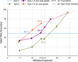
(a) Maze Navigation

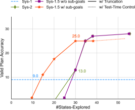
(b) Blocksworld

Figure 3: Comparison of System-$1.x$ Planner (with and without sub-goals) with a System-$1$ Planner and a System-$2$ Planner on (a) Maze Navigation and (b) Blocksworld. (a) System-$1.x$ with sub-goals matches or generally outperforms all baselines for Maze Navigation. (b) On out-of-distribution generalization in Blocksworld, System-$1.x$ with sub-goals leads to much higher plan accuracy at lower #States-Explored.

Study Setup.

In this first set of experiments, we compare our System-$1.x$ Planner with the following baselines (cf. Section 3.2) (1) a System-$1$ Planner, (2) a System-$2$ Planner, and (3) a System-$1.x$ Planner without sub-goal decomposition.

Results for Maze Navigation. Fig. 3(a) (cf. Table 3) shows the plan accuracy obtained by each planner at different #States-Explored. The values of #States-Explored are as described previously in Section 3.3. Based on this, we summarize our key findings.

• System-$1.x$ outperforms all baselines at all budgets. Without truncation or test-time control, System-$1.x$ ($x\!=\!0.5$) uses $13.6$ states on average. At this number of states, it obtains an accuracy of $70.4\%$, outperforming the System-$1$ Planner by 21% (48.7% $\rightarrow$ 70.4%), the System-$2$ Planner by 33% (37.2% $\rightarrow$ 70.4%), and the System-$1.x$ variant without sub-goal decomposition by 20% (50.0% $\rightarrow$ 70.4%). Next, to compare all methods at lower budgets (i.e., with #States-Explored of 5 and 10), we do state truncation (as described in Section 3.3) by limiting the search (generation) to a maximum number of states. We find that even at these lower budgets, System-$1.x$ continues to be significantly more accurate compared to baselines, pointing to an effective allocation of resources. Finally, System-$1.x$’s test-time control capability lets us increase compute to match that of System-$2$ by biasing the controller and solving more sub-goals with System-$2$. Doing so eventually transforms a System-$1.x$ Planner into a System-$2$ Planner with sub-goal decomposition, outperforming vanilla System-$2$ by 3% and achieving the highest accuracy of $96.7\%$ at 27.3 states. This highlights the effectiveness of our sub-goal decomposition (more details below).

• System-$1.x$ benefits from sub-goal decomposition. We validate the utility of sub-goal decomposition from two observations. First, the full System-$1.x$ outperforms the System-$1.x$ variant that does not perform sub-goal decomposition. Second, System-$2$ also benefits from sub-goal decomposition as shown by the maximum accuracy of 96.7% which is achieved via test-time control and biasing the controller to solve every sub-goal using System-$2$. However, note that System-$2$ with decomposition still applies System-$2$ planning to every step, making System-$1.x$ more performant at any given budget.

• System-$1$ is cheaper but not accurate. On one extreme of the plot, System-$1$ Planner is cheaper since it only explores the states that are part of its plan, amounting to an average of 3 states. However, this comes at a cost to performance: it also only achieves an accuracy of 49%. Another limitation of a System-$1$ Planner is that unlike System-$1.x$, it is not controllable and hence, there is no easy affordance for improving performance by exploring more states.

• System-$2$ is more accurate but expensive. On the other extreme, System-$2$ Planner achieves a maximum accuracy of 94% but explores a much higher 24.4 states in the process. While System-$2$ can be adapted to minimize #States-Explored, such adaptivity is only possible during inference via state-truncation. Test-time truncation of #States-Explored is typically ad-hoc and not preferable because the loss in performance will only increase as the plan length grows. This is in contrast to the System-$1.x$ Planner, which allows for systematic control of compute both at training-time (via a user-defined hybridization factor $x$), and at test-time (by biasing the controller).

Results for Blocksworld.

Fig. 3(b) (cf. Table 4) reports our results on Blocksworld (BW) that studies out-of-distribution generalization to longer plan lengths. Our first observation is that System-$1$ only obtains an accuracy of 9% and although System-$2$’s accuracy is higher at 28%, given the longer plan lengths, it also explores a significantly higher number of states (55).

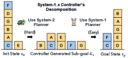
Figure 4: An example decomposition generated by System $1.5$ for Blocksworld. The adjacent blocks ‘C’ and ‘F’ (in the goal state) are separated by 4 blocks in the intital state. The controller generates an intermediate state $\mathcal{G}_{1}$ where blocks ‘C’ and ‘F’ are a block apart, with the sub-goal $s_{0}\rightarrow\mathcal{G}_{1}$ being harder (solved using System-$2$) and the sub-goal $\mathcal{G}_{1}\rightarrow s_{g}$ being easier and solved via System-$1$.

Thus, when we perform truncation to get lower values of #States-Explored, System-$2$’s accuracy drops to almost 0%. System-$1.x$ without sub-goal decomposition also does not work for OOD test points because the controller predicts almost all samples as hard and solves them using System-$2$. Hence, System-$1.x$ without sub-goal decomposition practically becomes a System-$2$ in such scenarios, suffering major losses to performance with truncation. However, in contrast to all baselines, System-$1.x$ with sub-goal decomposition can solve a larger fraction of problems at lower budgets (e.g., 25% at 30 states compared to System-$2$ Planner’s 13%) because of its ability to leverage a System-$1$ Planner for simpler sub-goals that have shorter plan lengths and are more likely to be in-distribution (refer to example in Fig. 4). At maximum #States-Explored, System-$1.x$ obtains comparable performance to a System-$2$ Planner. Overall, when testing on OOD data, the results in Fig. 3(b) highlight the key role that the System-$1.x$ controller plays in decomposing longer-horizon planning problems. Crucially, what is generally a weak System-$1$ Planner for harder, OOD goals can be used effectively to solve easier, ID sub-goals, thereby saving a lot of compute.

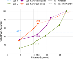
Figure 5: Performance of System-$1.x$ in conjunction with a symbolic (A^∗) System-$2$ Planner on Maze. The neuro-symbolic System-$1.x$ Planner matches if not outperforms A^∗ search with the same budget of #States-Explored, e.g., by 39% at 11.6 states.

4.2 Neuro-symbolic System-$1.x$ outperforms or matches A^∗ at all budgets

Study Setup.

While we primarily designed System-$1.x$ as a fully neural planner with all three components (System-$1$, $2$, and the controller) developed on top of the same LLM, we note that System-$1.x$ can also act as a neuro-symbolic planner. This can be achieved by using a symbolic solver like A^∗ as the System-$2$ component. We follow this setup to report results on the Maze Navigation task, again setting $x\!=\!0.5$.

Results.

Table 5 (cf. Table 5) compares the accuracy of all planners at different #States-Explored. Our main result is that the conclusions drawn with a fully neural System-$1.x$ also transfer to a neuro-symbolic System-$1.x$. Notably, at an average of 11.6 states, neuro-symbolic System-$1.x$ outperforms A^∗ by a large margin of 39% (31.0% $\rightarrow$ 70.5%). This can again be explained by the ineffectiveness of #States-Explored truncation for System-$2$ Planners, symbolic or neural. The trend is also consistent at all lower budgets. System-$1.x$ can be test-time controlled to obtain a near-perfect accuracy (99.2%), matching that of A^∗.

4.3 Analyses and Ablations of System-$1.x$ Planner

We conduct all analyses and ablations on the maze navigation task.

Train-time Control: System-$\mathbf{1.75}$ trades off efficiency for accuracy compared to System-$\bm{1.5}$.

One of the core strengths of our planner is its training-time controllability. The hybridization factor $x$ allows the user to specify the System-$1$ to System-$2$ balance they want in the final planner. To demonstrate this capability, we train a System-$1.75$ Planner by setting $x=0.75$. Table 6 (cf. Table 6) shows our results on the maze task. By default, System-$1.75$ uses $16.6$ states on average and obtains an accuracy of $75.7\%$, compared to System-$1.5$’s $70.4\%$ with a default average of 13.6 states (Table 3) i.e., a 5% gain at the cost of 3 more states.

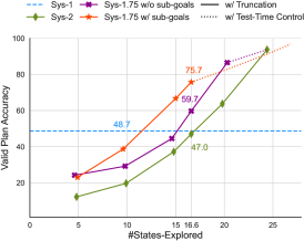
Figure 6: Train-time controllability of System-$1.x$ Planner by setting $x\!=\!0.75$. System-$1.75$ largely outperforms System-$2$. Compared to Fig. 3(a), System-$1.75$ yields an accuracy of 75.7% vs. 70.4% (with System-$1.5$) by utilizing 3 more states.

Thus, as we increase the value of $x$, the System-$1.x$ Planner will use more states and improve performance, converging to a System-$2$ Planner that additionally performs sub-goal decomposition. Compared to System-$2$, System-$1.75$ is again significantly more performant at all budgets (e.g., by $28\%$ at $16.6$ states) and eventually obtains the highest accuracy of $96.7\%$ when acting as a System-$2$ with sub-goals. This echoes our System-$1.5$ Planner findings, which also demonstrated similar gains at high budgets.

Broadly, these results showcase our controller’s effectiveness, which in turn validates our hardness measures and sub-goal decompositions. We further ablate features of the controller in Appendix B, comparing against a random controller, testing the effectiveness of the sliding window, and contrasting different hardness functions. These experiments confirm our choices in Section 3.4.

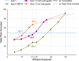
(a) System-$1.x$ with BFS

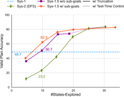
(b) System-$1.x$ with DFS

Figure 7: Comparison of System-$1.x$ Planner on Maze Navigation using (a) Breadth-First Search and (b) Depth-First Search traces. The System-$1.x$ Planner generally outperforms System-$2$ Planner in both cases, converging to System-$2$, showing robustness to the underlying search algorithm.

Generalizability: System-$1.x$ beats System-$2$ with all search algorithms (A^∗, DFS, BFS).

We conducted our main experiments by leveraging supervision from A^∗ traces. In this experiment, we show that System-$1.x$ is robust to different search algorithms, working with other options like Breadth First Search (BFS) and Depth First Search (DFS). First, note that for mazes, BFS explores all four actions (up, down, left, right) at each state and hence, on average, is the most expensive search strategy in terms of states explored. However, for an unweighted maze, BFS always generates optimal plans. DFS, on the other hand, explores fewer states because it returns the first valid plan, though that plan may not necessarily be optimal. Appendices C and C contains examples of BFS and DFS trajectories. Based on Fig. 7 (cf. Tables 7 and 8), we summarize our key findings:

• System-$1.x$ continues to outperform System-$2$ and ‘System-$1.x$ without sub-goal decomposition’ by large margins (e.g., up to 39% at 17.4 states for BFS and at 10 states for DFS), showcasing our planner’s flexibility to learn from different algorithms.

• System-$1.x$ closely resembles the behavior of the search algorithm it is trained on. For example, System-$1.x$ (BFS) is more accurate and generates a significantly higher number of optimal plans than System-$1.x$ (DFS) because the former is trained on optimal plans (refer to Table 2 for a study on validity versus optimality). In the process, however, System-$1.5$ (BFS) explores more states than System-$1.x$ (DFS), similar to their symbolic counterparts. Among the three algorithms studied in this paper, System-$1.x$ (A^∗) is the most accurate and efficient.

Qualitative Analysis of System $\bm{1}$, $\bm{2}$, and $\bm{1.x}$.

Fig. 8 shows an example from our test set where both System-$1$ and System-$2$ fail but System-$1.x$ succeeds. We consider a maze configuration where the plan length is quite long (8) and there is a solitary path to the goal, making the problem challenging for LLMs. We find that the System-$1$ Planner generates an incorrect plan that ignores the placement of the obstacles. On the other hand, the System-$2$ Planner avoids obstacles successfully initially but then takes a path that leads it to a dead end. It is unable to recover from that and the search does not terminate. Our System-$1.x$ Planner is, however, able to solve the problem successfully by first breaking it up into 3 sub-goals and solving the easy sub-goals close to the start state and the goal state using System-$1$ and the hard sub-goal in the middle (that includes a number of obstacles) with deliberate System-$2$ planning.

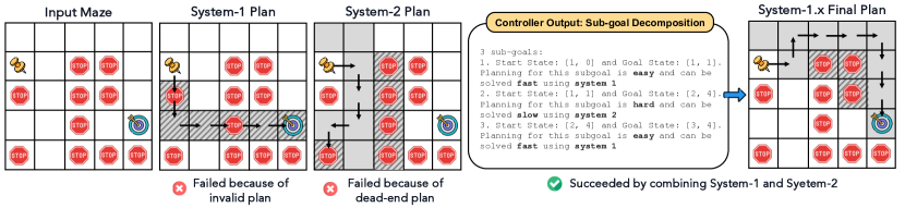
Figure 8: A qualitative example showing (1) a failure case for a System-$1$ Planner because it generates a plan through the obstacles, (2) a failure case for a System-$2$ Planner because the generated plan leads to a dead end and the model does not recover from it, and (3) a successful case for our System-$1.x$ Planner that solves the easy sub-goals near the start state and the goal state using System-$1$ and the hard sub-goal in the middle using System-$2$.

5 Discussion and Limitations

Comparison to Dual-Process Theories.

While System-$1.x$ draws on dual process theories of human cognition, it deviates in important ways. Crucially, most dual-process accounts hold that System-1 thinking occurs all the time, with System-2 occurring some of the time (Evans, 2003), whereas in our planning framework, the two are mutually exclusive. It is worth noting that, whether mutually exclusive or not, dual-process accounts require some control mechanism that triggers System-$2$; errors in this controller can lead to compounding errors downstream, which has also been posited as a theory for breakdowns in human cognition (Tversky and Kahneman, 1974; Gilovich et al., 2002). We also do not take a position on whether performing search by next-token prediction is optimal; indeed, our neuro-symbolic results in Fig. 5 indicate that System-$1.x$ is compatible with both neural implementations of search and symbolic search. Dual-process accounts also typically rely on some form of metacognition, where agents reason not only about the task, but also form a model of reasoning itself (Ganapini et al., 2022). This entails having not only a world model – in our case, how actions affect the agent’s state – but also a model of reasoning, i.e., how difficult a particular goal is or what kind of planning it might require. This is implemented by the controller, which routes between System-$1$ and System-$2$ based on the predicted hardness of a sub-goal.

Inferring $x$ from a State Budget.

In our work, we set $x$ in System-$1.x$, as well as the test-time control values, inducing a maximum budget. By fitting a function to the points in Figs. 3, 5, 6 and 7, one can easily go the other direction, mapping a particular state budget (or token budget) to a corresponding value of $x$ or a corresponding control value. This would allow users with specific compute constraints to ensure that the planner does not use more resources than allotted.

Limitations.

Firstly, like past work (Gandhi et al., 2024; Lehnert et al., 2024), our work focuses on fully-observable and deterministic domains; however, many real-world problems are partially-observable and non-deterministic. Secondly, our method is based on model-generated sub-goals; we find in Section 4.1 that System-$2$ also benefits from sub-goals, indicating that they are generally beneficial to all methods. Similarly, System-$1.x$ relies on a relative ranking of sub-goals by hardness; this can entail variable performance if the sub-goals are all easy or all hard (in absolute terms), in which case System-$1.x$ may lose efficiency, solving the most difficult of the easy goals with System-$2$ when System-$1$ would suffice, or lose performance, solving the easiest of a set of hard sub-goals with System-$1$ despite them requiring System-$2$. This could be remedied by introducing an absolute threshold on hardness; however, this would entail finding that threshold using validation data, which our current method avoids. Finally, System-$1.x$ training involves creating data with a sliding window of System-$2$ timesteps by assigning each sub-goal to System-$1$ or System-$2$. While this empirically works well for the problems we study, long plans with hundreds or thousands of steps might require more windows.

6 Related Work

Combining LLMs and Symbolic Planners.

Despite the widespread success of LLMs in complex problem-solving, a large body of recent work has highlighted their shortcomings on long-horizon planning problems (Valmeekam et al., 2023, 2024; Pallagani et al., 2023; Momennejad et al., 2024; Hirsch et al., 2024; Zheng et al., 2024; Aghzal et al., 2023), persisting across popular prompting techniques like Chain-of-Thought (Wei et al., 2022), ReAct (Yao et al., 2022), and Reflexion (Shinn et al., 2024). These methods can largely be grouped into System-$1$ inference-time methods in which the LLM does not search, backtrack, or learn from incorrect actions. Systematic search is either not performed at all or delegated to symbolic solvers (e.g., Liu et al., 2023; Pan et al., 2023; Xie et al., 2023, discussed further below), thus deviating from the focus of this work on equipping LLMs to solve harder planning problems via search.

More related to our work are inference-time methods that do involve planning, tree search, and backtracking. These System-$2$-inspired methods have a search algorithm that operates on top of and guides an LLM with reward models, value functions, or verifiers (Hao et al., 2023; Yao et al., 2024; Besta et al., 2024; Zhou et al., 2023; Sel et al., 2023; Koh et al., 2024). In a similar spirit, neuro-symbolic planning systems like LLM-Modulo Frameworks (Kambhampati et al., 2024) have emerged that combine LLMs with symbolic planners (Nye et al., 2021; Liu et al., 2023; Pan et al., 2023; Xie et al., 2023; Kambhampati et al., 2024; Zuo et al., 2024) System-$1.x$ differs from this class of inference-time methods in two major ways. Firstly, it is a training-time method that teaches the LLM to search, with the goal of enhancing the LLM’s intrinsic planning capabilities and discovering more effective search strategies, making it self-contained (as opposed to complex inference-time methods relying on external modules). Secondly, it is also a hybrid system that can alternate between System-$1$ and System-$2$-style planning, whereas past work is capable of one or the other, but not both. Notably, this kind of hybridization distinguishes System-$1.x$ from other work that either creates hybrids between weaker and stronger models in the form of model cascades (Lin et al., 2024; Yue et al., 2023) or between neural and symbolic methods (e.g., LLM-Modulo frameworks).

LLMs Generating Plans.

Methods combining LLMs and symbolic planners need some channel of communication between the LLM and the symbolic planning component. This is usually a value function or reward model producing a single score for a state, making the success of the method contingent on the quality of the reward model, or the LLM’s ability to act as a value function (as in Yao et al. (2024); Lightman et al. (2023)). Furthermore, off-loading planning or search adds additional modules at test-time that may not always be available for certain domains. It also assumes that the model’s representation is already sufficient for the task and complicates finetuning the representation, since externalized search is typically non-differentiable. In an attempt to mitigate such concerns, a second line of work removes the dependency on separate reward models and external tools and teaches LLMs to conduct search by themselves (Yang et al., 2022; Gandhi et al., 2024; Lehnert et al., 2024). For example, Gandhi et al. (2024) introduce Stream-of-Search (SoS), which teaches LLMs to search by verbalizing trajectories and Lehnert et al. (2024) propose Searchformer, that learns from A^∗ search dynamics. This line of work predates LLMs: Anthony et al. (2017) generate data from tree search which they use to iteratively train a neural model to perform System-$1$ planning. However, Gandhi et al. (2024) and Lehnert et al. (2024) differ from our work in that their final models are System-$2$-only, incurring a high computational cost for all examples and states by performing full planning at all times, whereas our method is a hybrid between Systems $1$ and $2$, dynamically allocating computation to more difficult parts of the plan. Moreover, to meet user budget constraints, System-$2$-only methods also have to rely on approaches like post-hoc truncation while System-$1.x$ offers more systematic controllability via its controller.

7 Conclusion

We introduced the System-$1.x$ Planner, a novel neural planner that adaptively interleaves quick and cost-efficient System-$1$ planning with more costly but performant System-$2$ planning. On two tasks, we showed that our method results in strong performance across a range of budgets: on Mazes, System-$1.x$ beats obtains the best performance at every budget, and on Blocksworld it outperforms System-$2$ at all budgets except the highest, where it is comparable. System-$1.x$ Planner achieves this by decomposing problems into sub-goals and intelligently allocating System-$2$’s additional resources to harder sub-goals while allowing System-$1$ to quickly solve the easier ones. Furthermore, our method is adaptable, allowing users to control the cost and performance by specifying the degree to which the planner relies on System-$2$. In our analysis, we find that System-$1.x$ is controllable, generalizes to various search algorithms, and performs better out-of-distribution. We also ablate choices to our training data creation, including the choice of the hardness function and the search algorithm, finding System-$1.x$ is robust to such changes.

Appendix A Additional Details of System-$1.x$ Planner

Background on A^∗.

A^∗ is an informed search algorithm that decides the next best state to expand with a function $f(n)=g(n)+t(n)$ that considers (1) the cost $g(n)$ from the start state to the current state $n$, and (2) a heuristic function $t(n)$ that gives an estimate of the cost from state $n$ to the goal. Note that A^∗ is optimal if the heuristic $t(n)$ is admissible (i.e., $t(n)\leq t^{*}(n)$ which means that the heuristic never overestimates the true cost to the goal $h^{*}(n)$) and consistent (i.e., $t(n)\leq c(n,n^{\prime})+t(n^{\prime})$ for all states $n$ and its successor $n^{\prime}$ and $c$ is the cost to transition from $n$ to $n^{\prime}$). For the Maze Navigation task, Manhattan Distance is an example of such an admissible heuristic, and hence $A^{*}$ with it will always generate optimal plans.

System-$\mathbf{2}$ Planner for Maze Navigation.

We implement a System-$2$ Planner for the Maze domain by verbalizing all possible explorations at each state, including the ones that lead to invalid states (i.e., outside the maze, have obstacles, or have already been visited). See example in Appendix C.

System-$\mathbf{2}$ Planner for Blocksworld.

In contrast to the Maze domain, the number of actions at each state in Blocksworld problem is directly proportional to the total number of blocks. Consequently, the number of possible states that can be explored (both valid and invalid) is significantly larger in this domain, often exceeding the maximum input token budgets of standard LLMs (in our case, 8096 tokens). Therefore, when verbalizing the search trajectories $\mathcal{T}$ in $\mathcal{D}_{\textrm{Sys2}}$ using A^∗ search to train System-$2$ Planner, we cap the number of valid and invalid states explored to 3 and 2 respectively. The verbalized valid states are chosen by picking the top-3 scored states as per the A^∗ heuristic (that computes the number of mismatches between the start state and the goal state), while (up to) 2 invalid states are chosen randomly to make the model learn from mistakes. Refer to Appendix C for an example.

Appendix B Additional Results

System-$1.x$ Controller outperforms a random controller. In Table 1, we compare our System $1.5$ controller with a random controller that arbitrarily chooses 50% problems to be solved by System-$2$. Our trained controller outperforms the random controller by a significant 10%.

	Accuracy
System $1.5$ (w/ random controller)	70.5
System $1.5$ (w/ our controller)	79.5

Table 1: Comparison of our trained controller in System-$1.x$ Planner with a controller that randomly chooses $x\%$ of problems to solve with System-$2$.

Analyses of System-$1.x$ Controller.

In this section, we analyze the different components of our System-$1.x$ controller.

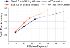
Figure 9: Comparison of System-$1.x$ Planner with and without sliding window-based sub-goal decomposition on the Maze Navigation task. Sliding window-based decomposition outperforms the variant without it at all budgets.

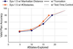
Figure 10: Comparison of two hardness functions (Manhattan Distance and #Obstacles) for Maze Navigation. Both yield comparable results, with #Obstacles being slightly better.

• Effectiveness of Sliding Window Decomposition. Recall that we generated training data for the controller by using a sliding window approach that assigned a contiguous $x$% of the plan to System-$2$ according to a hardness function. Here, we evaluate the effectiveness of this approach by comparing it to a System-$1.x$ variant without the sliding window decomposition. In this variant, the $x$% System-$2$ allocation can either be at the beginning or at the end of the plan but not in the middle, resulting in a maximum of two decompositions instead of three. As shown in Fig. 9, our sliding window variant not only obtains higher accuracy but is also far more efficient. This is because with three decompositions, a weaker System-$1$ Planner can be used to solve two granular sub-goals (instead of one) and hence is more likely to succeed.

• Comparison of Hardness Functions. Our experiments on maze used the number of obstacles in a sub-maze as the hardness function. In Table 10, we compare it to Manhattan Distance, which rates goals that are further away (according to the distance function) as more difficult. We observe that both functions lead to comparable performance, with obstacles being slightly more efficient. Taken together with the previous experiment, these results quantify the influence of two essential inputs to the controller’s training: hardness function and the decomposition strategy.

	Valid Plan	Optimal Plan	#States-Explored
System-$1.x$ (w/o sub-goals)	33.5	33.2	4.8
System-$1.x$ (w/o sub-goals)	38.2	38.0	9.7
System-$1.x$ (w/o sub-goals)	62.2	61.7	15.0
System-$1.x$ (w/o sub-goals)	79.5	78.7	17.4
System-$1.x$ (w/ sub-goals)	30.5	30.2	4.5
System-$1.x$ (w/ sub-goals)	56.2	53.7	10.0
System-$1.x$ (w/ sub-goals)	70.4	61.5	13.6

Table 2: Comparison of Valid Plan Accuracy and Optimal Plan Accuracy for System-$1.x$ Planner in Maze Navigation using A^∗ search. While not using sub-goal decomposition nearly guarantees optimality, using sub-goal decomposition may generate plans that are sub-optimal.

Optimality of System-$1.x$.

In Table 2, we compare the optimality and validity of the plans generated by our System-$1.x$ Planner. While System-$1.x$ without sub-goal decomposition generates plans that are almost always optimal, we observe that sub-goal decomposition may sometimes hurt optimality. This happens because the sub-goals generated by the controller may not always lie on the optimal path.

Appendix C Prompts and Examples

See the subsequent pages for prompts and examples from both domains.

Appendix D Tables corresponding to Result Figures

In the tables below, we report the accuracies corresponding to all the plots in the paper.

	Accuracy	#States-Explored
System-$1$	48.7	3.1
System-$2$ (truncated)	12.2	4.8
System-$2$ (truncated)	19.7	9.9
System-$2$ (truncated)	37.2	13.6
System-$2$ (truncated)	37.2	14.8
System-$2$ (truncated)	63.7	19.8
System-$2$ (default)	93.7	24.4
System-$1.5$ w/o sub-goal (truncated)	33.5	4.8
System-$1.5$ w/o sub-goal (truncated)	38.2	9.7
System-$1.5$ w/o sub-goal (truncated)	50.0	13.4
System-$1.5$ w/o sub-goal (truncated)	62.2	15.0
System-$1.5$ w/o sub-goal (default)	79.5	17.4
System-$1.5$ w/o sub-goal (test-time controlled)	83.7	20.0
System-$1.5$ (w/o sub-goal) (test-time controlled)	93.7	24.4
System-$1.5$ w/ sub-goal (truncated)	30.5	4.5
System-$1.5$ w/ sub-goal (truncated)	56.2	10.0
System-$1.5$ w/ sub-goal (default)	70.4	13.6
System-$1.5$ w/ sub-goal (test-time controlled)	82.2	19.9
System-$1.5$ w/ sub-goal (test-time controlled)	92.2	24.4
System-$1.5$ w/ sub-goal (test-time controlled)	96.7	27.3

Table 3: Comparison of System-$1.x$ Planner ($x=0.5$) with all baselines on Maze Navigation (corresponding to Fig. 3(a)). The blue rows indicate accuracy obtained by all methods when #States-Explored is matched to that of System $1.5$ with sub-goals. The green rows indicate accuracy obtained when #States-Explored is maximized. All tables, henceforth, will use the same color coding.

	Accuracy	#States-Explored
System $1$	9.0	4.5
System $2$ (truncated)	0.0	9.8
System $2$ (truncated)	0.0	19.9
System $2$ (truncated)	13.0	29.3
System $2$ (truncated)	27.0	38.2
System $2$ (default)	28.0	55.5
System-$1.5$ w/o sub-goal (truncated)	0.0	9.8
System-$1.5$ w/o sub-goal (truncated)	0.0	19.9
System-$1.5$ w/o sub-goal (truncated)	13.0	29.3
System-$1.5$ w/o sub-goal (truncated)	27.0	38.0
System-$1.5$ w/o sub-goal (default)	28.0	55.1
System-$1.5$ w/ sub-goal (truncated)	1.5	9.6
System-$1.5$ w/ sub-goal (truncated)	17.5	20.0
System-$1.5$ w/ sub-goal (truncated)	25.0	30.0
System-$1.5$ w/ sub-goal (default)	25.0	38.3
System-$1.5$ w/ sub-goal (test-time controlled)	26.0	53.5

Table 4: Comparison of System-$1.x$ Planner ($x=0.5$) with all baselines on Blocksworld (corresponding to Fig. 3(b)).

	Accuracy	#States-Explored
A∗ (truncated)	12.5	4.8
A∗ (truncated)	22.5	9.8
A∗ (truncated)	31.0	11.3
A∗ (truncated)	42.0	14.5
A∗ (truncated)	67.7	19.8
A∗ (default)	100.0	22.4
System-$1.5$ w/o sub-goal (truncated)	33.0	4.8
System-$1.5$ w/o sub-goal (truncated)	40.2	9.8
System-$1.5$ w/o sub-goal (truncated)	45.7	11.5
System-$1.5$ w/o sub-goal (truncated)	65.7	14.9
System-$1.5$ w/o sub-goal (default)	84.2	16.5
System-$1.5$ w/o sub-goal (test-time controlled)	94.0	20.0
System-$1.5$ w/o sub-goal (test-time controlled)	100.0	22.4
System-$1.5$ w/ sub-goal (truncated)	30.5	4.5
System-$1.5$ w/ sub-goal (truncated)	58.7	10.0
System-$1.5$ (default)	70.5	11.6
System-$1.5$ w/ sub-goal (test-time controlled)	76.0	14.8
System-$1.5$ w/ sub-goal (test-time controlled)	89.7	19.9
System-$1.5$ w/ sub-goal (test-time controlled)	99.2	23.9

Table 5: Comparison of Neuro-symbolic System-$1.x$ Planner ($x=0.5$) with all baselines on Maze Navigation (corresponding to Fig. 5).

	Accuracy	#States-Explored
System-$2$ (truncated)	12.2	4.8
System-$2$ (truncated)	19.7	9.9
System-$2$ (truncated)	37.2	14.8
System-$2$ (truncated)	47.0	16.6
System-$2$ (truncated)	63.7	19.8
System-$2$ (default)	93.7	24.4
System-$1.75$ w/o sub-goal (truncated)	24.2	4.6
System-$1.75$ w/o sub-goal (truncated)	29.2	9.8
System-$1.75$ w/o sub-goal (truncated)	44.5	14.6
System-$1.75$ w/o sub-goal (default)	59.7	16.6
System-$1.75$ w/o sub-goal (default)	86.5	20.3
System-$1.75$ w/o sub-goal (test-time controlled)	93.7	24.4
System-$1.75$ w/ sub-goal (truncated)	23.0	4.9
System-$1.75$ w/ sub-goal (truncated)	38.7	9.6
System-$1.75$ w/ sub-goal (truncated)	66.7	15.0
System-$1.75$ w/ sub-goal (default)	75.7	16.6
System-$1.75$ w/ sub-goal (test-time controlled)	82.0	19.9
System-$1.75$ w/ sub-goal (test-time controlled)	91.2	24.4
System-$1.75$ w/ sub-goal (test-time controlled)	96.7	26.8

Table 6: Comparison of System-$1.x$ Planner ($x\!=\!0.75$) with all baselines on Maze Navigation (corresponding to Fig. 6).

	Accuracy	#States-Explored
System-$2$ (truncated)	11.7	9.4
System-$2$ (truncated)	28.0	17.4
System-$2$ (truncated)	28.0	19.9
System-$2$ (truncated)	56.2	29.7
System-$2$ (default)	91.2	39.8
System-$1.5$ w/o sub-goal (truncated)	35.2	9.6
System-$1.5$ w/o sub-goal (truncated)	45.0	17.2
System-$1.5$ w/o sub-goal (truncated)	52.5	19.9
System-$1.5$ w/o sub-goal (default)	77.2	26.9
System-$1.5$ w/o sub-goal (test-time controlled)	81.2	30.0
System-$1.5$ w/o sub-goal (test-time controlled)	91.2	39.8
System-$1.5$ w/ sub-goal (truncated)	43.0	9.8
System-$1.5$ w/ sub-goal (default)	67.0	17.4
System-$1.5$ w/ sub-goal (test-time controlled)	78.5	29.7
System-$1.5$ w/ sub-goal (test-time controlled)	86.5	39.9
System-$1.5$ w/ sub-goal (test-time controlled)	91.7	45.4

Table 7: Comparison of System-$1.x$ Planner ($x\!=\!0.5$ and BFS) with all baselines on Maze Navigation (corresponding to Fig. 7(a)).

	Valid Acc	Avg States
System-$2$ (truncated)	11.7	4.7
System-$2$ (truncated)	23.2	9.7
System-$2$ (truncated)	42.0	14.5
System-$2$ (truncated)	69.7	19.8
System-$2$ (truncated)	81.2	25.0
System-$2$ (default)	83.5	30.4
System-$1.5$ w/o sub-goal (truncated)	36.0	4.7
System-$1.5$ w/o sub-goal (truncated)	50.7	9.8
System-$1.5$ w/o sub-goal (truncated)	73.2	15.0
System-$1.5$ w/o sub-goal (default)	74.0	18.7
System-$1.5$ w/o sub-goal (test-time controlled)	76.3	19.8
System-$1.5$ w/o sub-goal (test-time controlled)	81.2	25.0
System-$1.5$ w/o sub-goal (test-time controlled)	83.5	30.4
System-$1.5$ (truncated)	40.2	4.5
System-$1.5$ (default)	62.3	10.0
System-$1.5$ (test-time controlled)	76.3	14.9
System-$1.5$ (test-time controlled)	79.7	20.0
System-$1.5$ (test-time controlled)	82.7	33.6

Table 8: Comparison of System-$1.x$ Planner ($x\!=\!0.5$ and DFS) with all baselines on Maze Navigation (corresponding to Fig. 7(b)).

	Accuracy	#States-Explored
System-$1.5$ w/o Sliding Window (truncated)	27.5	4.6
System-$1.5$ w/o Sliding Window (truncated)	45.2	10.0
System-$1.5$ w/o Sliding Window (default)	67.2	17.0
System-$1.5$ w/o Sliding Window (test-time controlled)	72.1	20.0
System-$1.5$ w/o Sliding Window (test-time controlled)	77.2	25.0
System-$1.5$ w/o Sliding Window (test-time controlled)	83.2	30.0
System-$1.5$ w/o Sliding Window (test-time controlled)	90.0	35.3
System-$1.5$ w/ Sliding Window (truncated)	30.5	4.5
System-$1.5$ w/ Sliding Window (truncated)	56.2	10.0
System-$1.5$ w/ Sliding Window (default)	70.4	13.6
System-$1.5$ w/ Sliding Window (test-time controlled)	82.2	19.9
System-$1.5$ w/ Sliding Window (test-time controlled)	92.2	24.4
System-$1.5$ w/ Sliding Window (test-time controlled)	96.7	27.3

Table 9: Comparison of System-$1.x$ Planner with and without sliding window decomposition (corresponding to Fig. 10).

	Accuracy	#States-Explored
System-$1.5$ w/o sub-goal (#Obstacles)	33.5	4.8
System-$1.5$ w/o sub-goal (#Obstacles)	38.2	9.7
System-$1.5$ w/o sub-goal (#Obstacles)	50.0	13.4
System-$1.5$ w/o sub-goal (#Obstacles)	62.2	15.0
System-$1.5$ w/o sub-goal (#Obstacles)	79.5	17.4
System-$1.5$ w/o sub-goal (#Obstacles)	83.7	20.0
System-$1.5$ w/o sub-goal (#Obstacles)	93.7	24.4
System-$1.5$ w/o sub-goal (Manhattan)	31.7	4.8
System-$1.5$ w/o sub-goal (Manhattan)	54.5	15.0
System-$1.5$ w/o sub-goal (Manhattan)	35.2	10.0
System-$1.5$ w/o sub-goal (Manhattan)	80.0	18.8
System-$1.5$ w/o sub-goal (Manhattan)	81.5	19.9
System-$1.5$ w/o sub-goal (Manhattan)	93.7	24.4

Table 10: Comparison of two hardness functions (Manhattan Distance and #Obstacles) for Maze Navigation (corresponding to Fig. 10).

References

- Aghzal et al. (2023) Mohamed Aghzal, Erion Plaku, and Ziyu Yao. Can large language models be good path planners? a benchmark and investigation on spatial-temporal reasoning. arXiv preprint arXiv:2310.03249, 2023. URL https://arxiv.org/abs/2310.03249.
- Ahn et al. (2022) Michael Ahn, Anthony Brohan, Noah Brown, Yevgen Chebotar, Omar Cortes, Byron David, Chelsea Finn, Chuyuan Fu, Keerthana Gopalakrishnan, Karol Hausman, et al. Do as i can, not as i say: Grounding language in robotic affordances. arXiv preprint arXiv:2204.01691, 2022. URL https://arxiv.org/abs/2204.01691.
- Anthony et al. (2017) Thomas Anthony, Zheng Tian, and David Barber. Thinking fast and slow with deep learning and tree search. Advances in neural information processing systems, 30, 2017. URL https://proceedings.neurips.cc/paper/2017/hash/d8e1344e27a5b08cdfd5d027d9b8d6de-Abstract.html.
- Bachmann and Nagarajan (2024) Gregor Bachmann and Vaishnavh Nagarajan. The pitfalls of next-token prediction. arXiv preprint arXiv:2403.06963, 2024. URL https://arxiv.org/abs/2403.06963.
- Besta et al. (2024) Maciej Besta, Nils Blach, Ales Kubicek, Robert Gerstenberger, Michal Podstawski, Lukas Gianinazzi, Joanna Gajda, Tomasz Lehmann, Hubert Niewiadomski, Piotr Nyczyk, et al. Graph of thoughts: Solving elaborate problems with large language models. In Proceedings of the AAAI Conference on Artificial Intelligence, volume 38, pages 17682–17690, 2024. URL https://ojs.aaai.org/index.php/AAAI/article/view/29720.
- Bohnet et al. (2024) Bernd Bohnet, Azade Nova, Aaron T Parisi, Kevin Swersky, Katayoon Goshvadi, Hanjun Dai, Dale Schuurmans, Noah Fiedel, and Hanie Sedghi. Exploring and benchmarking the planning capabilities of large language models. arXiv preprint arXiv:2406.13094, 2024.
- Bubeck et al. (2023) Sébastien Bubeck, Varun Chandrasekaran, Ronen Eldan, Johannes Gehrke, Eric Horvitz, Ece Kamar, Peter Lee, Yin Tat Lee, Yuanzhi Li, Scott Lundberg, et al. Sparks of artificial general intelligence: Early experiments with gpt-4. arXiv preprint arXiv:2303.12712, 2023. URL https://arxiv.org/abs/2303.12712.
- Dziri et al. (2023) Nouha Dziri, Ximing Lu, Melanie Sclar, Xiang Lorraine Li, Liwei Jiang, Bill Yuchen Lin, Sean Welleck, Peter West, Chandra Bhagavatula, Ronan Le Bras, et al. Faith and fate: Limits of transformers on compositionality. Advances in Neural Information Processing Systems, 36, 2023. URL https://proceedings.neurips.cc/paper_files/paper/2023/hash/deb3c28192f979302c157cb653c15e90-Abstract-Conference.html.
- Evans (2003) Jonathan St BT Evans. In two minds: dual-process accounts of reasoning. Trends in cognitive sciences, 7(10):454–459, 2003.
- Ganapini et al. (2022) M Bergamaschi Ganapini, Murray Campbell, Francesco Fabiano, Lior Horesh, Jon Lenchner, Andrea Loreggia, Nicholas Mattei, Francesca Rossi, Biplav Srivastava, and Kristen Brent Venable. Thinking fast and slow in ai: The role of metacognition. In International Conference on Machine Learning, Optimization, and Data Science, pages 502–509. Springer, 2022. URL https://arxiv.org/abs/2110.01834.
- Gandhi et al. (2024) Kanishk Gandhi, Denise Lee, Gabriel Grand, Muxin Liu, Winson Cheng, Archit Sharma, and Noah D Goodman. Stream of search (sos): Learning to search in language. arXiv preprint arXiv:2404.03683, 2024. URL https://arxiv.org/abs/2404.03683.
- Gilovich et al. (2002) Thomas Gilovich, Dale Griffin, and Daniel Kahneman. Heuristics and biases: The psychology of intuitive judgment. Cambridge university press, 2002.
- Hao et al. (2023) Shibo Hao, Yi Gu, Haodi Ma, Joshua Hong, Zhen Wang, Daisy Wang, and Zhiting Hu. Reasoning with language model is planning with world model. In Proceedings of the 2023 Conference on Empirical Methods in Natural Language Processing, pages 8154–8173, 2023.
- Hirsch et al. (2024) Eran Hirsch, Guy Uziel, and Ateret Anaby-Tavor. What’s the plan? evaluating and developing planning-aware techniques for llms. arXiv preprint arXiv:2402.11489, 2024. URL https://arxiv.org/abs/2402.11489.
- Hu et al. (2021) Edward J Hu, Phillip Wallis, Zeyuan Allen-Zhu, Yuanzhi Li, Shean Wang, Lu Wang, Weizhu Chen, et al. Lora: Low-rank adaptation of large language models. In International Conference on Learning Representations, 2021. URL https://arxiv.org/abs/2106.09685.
- Jiang et al. (2023) Albert Q Jiang, Alexandre Sablayrolles, Arthur Mensch, Chris Bamford, Devendra Singh Chaplot, Diego de las Casas, Florian Bressand, Gianna Lengyel, Guillaume Lample, Lucile Saulnier, et al. Mistral 7b. arXiv preprint arXiv:2310.06825, 2023. URL https://arxiv.org/abs/2310.06825.
- Kahneman (2011) Daniel Kahneman. Thinking, fast and slow. macmillan, 2011.
- Kambhampati et al. (2024) Subbarao Kambhampati, Karthik Valmeekam, Lin Guan, Kaya Stechly, Mudit Verma, Siddhant Bhambri, Lucas Saldyt, and Anil Murthy. Llms can’t plan, but can help planning in llm-modulo frameworks. arXiv preprint arXiv:2402.01817, 2024. URL https://arxiv.org/abs/2402.01817.
- Koh et al. (2024) Jing Yu Koh, Stephen McAleer, Daniel Fried, and Ruslan Salakhutdinov. Tree search for language model agents. Preprint, 2024.
- Lehnert et al. (2024) Lucas Lehnert, Sainbayar Sukhbaatar, Paul Mcvay, Michael Rabbat, and Yuandong Tian. Beyond a*: Better planning with transformers via search dynamics bootstrapping. arXiv preprint arXiv:2402.14083, 2024. URL https://arxiv.org/abs/2402.14083.
- Lightman et al. (2023) Hunter Lightman, Vineet Kosaraju, Yuri Burda, Harrison Edwards, Bowen Baker, Teddy Lee, Jan Leike, John Schulman, Ilya Sutskever, and Karl Cobbe. Let’s verify step by step. In The Twelfth International Conference on Learning Representations, 2023. URL https://arxiv.org/abs/2305.20050.
- Lin et al. (2024) Bill Yuchen Lin, Yicheng Fu, Karina Yang, Faeze Brahman, Shiyu Huang, Chandra Bhagavatula, Prithviraj Ammanabrolu, Yejin Choi, and Xiang Ren. Swiftsage: A generative agent with fast and slow thinking for complex interactive tasks. Advances in Neural Information Processing Systems, 36, 2024. URL https://proceedings.neurips.cc/paper_files/paper/2023/hash/4b0eea69deea512c9e2c469187643dc2-Abstract-Conference.html.
- Liu et al. (2023) Bo Liu, Yuqian Jiang, Xiaohan Zhang, Qiang Liu, Shiqi Zhang, Joydeep Biswas, and Peter Stone. Llm+ p: Empowering large language models with optimal planning proficiency. arXiv preprint arXiv:2304.11477, 2023. URL https://arxiv.org/abs/2304.11477.
- Momennejad et al. (2024) Ida Momennejad, Hosein Hasanbeig, Felipe Vieira Frujeri, Hiteshi Sharma, Nebojsa Jojic, Hamid Palangi, Robert Ness, and Jonathan Larson. Evaluating cognitive maps and planning in large language models with cogeval. Advances in Neural Information Processing Systems, 36, 2024. URL https://proceedings.neurips.cc/paper_files/paper/2023/hash/dc9d5dcf3e86b83e137bad367227c8ca-Abstract-Conference.html.
- Nye et al. (2021) Maxwell Nye, Michael Tessler, Josh Tenenbaum, and Brenden M Lake. Improving coherence and consistency in neural sequence models with dual-system, neuro-symbolic reasoning. Advances in Neural Information Processing Systems, 34:25192–25204, 2021. URL https://proceedings.neurips.cc/paper/2021/hash/d3e2e8f631bd9336ed25b8162aef8782-Abstract.html.
- Pallagani et al. (2023) Vishal Pallagani, Bharath Muppasani, Keerthiram Murugesan, Francesca Rossi, Biplav Srivastava, Lior Horesh, Francesco Fabiano, and Andrea Loreggia. Understanding the capabilities of large language models for automated planning. arXiv preprint arXiv:2305.16151, 2023. URL https://arxiv.org/abs/2305.16151.
- Pan et al. (2023) Liangming Pan, Alon Albalak, Xinyi Wang, and William Wang. Logic-LM: Empowering large language models with symbolic solvers for faithful logical reasoning. In Houda Bouamor, Juan Pino, and Kalika Bali, editors, Findings of the Association for Computational Linguistics: EMNLP 2023, pages 3806–3824, Singapore, December 2023. Association for Computational Linguistics. doi: 10.18653/v1/2023.findings-emnlp.248. URL https://aclanthology.org/2023.findings-emnlp.248.
- Prasad et al. (2024) Archiki Prasad, Alexander Koller, Mareike Hartmann, Peter Clark, Ashish Sabharwal, Mohit Bansal, and Tushar Khot. Adapt: As-needed decomposition and planning with language models. In Findings of the Association for Computational Linguistics: NAACL 2024, pages 4226–4252, 2024.
- Russell and Norvig (2016) Stuart J Russell and Peter Norvig. Artificial intelligence: a modern approach. Pearson, 2016.
- Sel et al. (2023) Bilgehan Sel, Ahmad Al-Tawaha, Vanshaj Khattar, Lu Wang, Ruoxi Jia, and Ming Jin. Algorithm of thoughts: Enhancing exploration of ideas in large language models. arXiv preprint arXiv:2308.10379, 2023. URL https://arxiv.org/abs/2308.10379.
- Shinn et al. (2024) Noah Shinn, Federico Cassano, Ashwin Gopinath, Karthik Narasimhan, and Shunyu Yao. Reflexion: Language agents with verbal reinforcement learning. Advances in Neural Information Processing Systems, 36, 2024. URL https://proceedings.neurips.cc/paper_files/paper/2023/hash/1b44b878bb782e6954cd888628510e90-Abstract-Conference.html.
- Tversky and Kahneman (1974) Amos Tversky and Daniel Kahneman. Judgment under uncertainty: Heuristics and biases: Biases in judgments reveal some heuristics of thinking under uncertainty. science, 185(4157):1124–1131, 1974.
- Valmeekam et al. (2023) Karthik Valmeekam, Matthew Marquez, Sarath Sreedharan, and Subbarao Kambhampati. On the planning abilities of large language models-a critical investigation. Advances in Neural Information Processing Systems, 36:75993–76005, 2023. URL https://proceedings.neurips.cc/paper_files/paper/2023/hash/efb2072a358cefb75886a315a6fcf880-Abstract-Conference.html.
- Valmeekam et al. (2024) Karthik Valmeekam, Matthew Marquez, Alberto Olmo, Sarath Sreedharan, and Subbarao Kambhampati. Planbench: An extensible benchmark for evaluating large language models on planning and reasoning about change. Advances in Neural Information Processing Systems, 36, 2024. URL https://proceedings.neurips.cc/paper_files/paper/2023/hash/7a92bcdede88c7afd108072faf5485c8-Abstract-Datasets_and_Benchmarks.html.
- Vaswani et al. (2017) Ashish Vaswani, Noam Shazeer, Niki Parmar, Jakob Uszkoreit, Llion Jones, Aidan N Gomez, Łukasz Kaiser, and Illia Polosukhin. Attention is all you need. Advances in neural information processing systems, 30, 2017.
- Wason and Evans (1974) Peter C Wason and J St BT Evans. Dual processes in reasoning? Cognition, 3(2):141–154, 1974.
- Wei et al. (2022) Jason Wei, Xuezhi Wang, Dale Schuurmans, Maarten Bosma, Fei Xia, Ed Chi, Quoc V Le, Denny Zhou, et al. Chain-of-thought prompting elicits reasoning in large language models. Advances in neural information processing systems, 35:24824–24837, 2022. URL https://proceedings.neurips.cc/paper_files/paper/2022/hash/9d5609613524ecf4f15af0f7b31abca4-Abstract-Conference.html.
- Xie et al. (2023) Yaqi Xie, Chen Yu, Tongyao Zhu, Jinbin Bai, Ze Gong, and Harold Soh. Translating natural language to planning goals with large-language models. arXiv preprint arXiv:2302.05128, 2023. URL https://arxiv.org/abs/2302.05128.
- Yang et al. (2022) Mengjiao Sherry Yang, Dale Schuurmans, Pieter Abbeel, and Ofir Nachum. Chain of thought imitation with procedure cloning. Advances in Neural Information Processing Systems, 35:36366–36381, 2022. URL https://arxiv.org/abs/2205.10816.
- Yao et al. (2022) Shunyu Yao, Jeffrey Zhao, Dian Yu, Nan Du, Izhak Shafran, Karthik R Narasimhan, and Yuan Cao. React: Synergizing reasoning and acting in language models. In The Eleventh International Conference on Learning Representations, 2022. URL https://arxiv.org/abs/2210.03629.
- Yao et al. (2024) Shunyu Yao, Dian Yu, Jeffrey Zhao, Izhak Shafran, Tom Griffiths, Yuan Cao, and Karthik Narasimhan. Tree of thoughts: Deliberate problem solving with large language models. Advances in Neural Information Processing Systems, 36, 2024. URL https://arxiv.org/abs/2305.10601.
- Yue et al. (2023) Murong Yue, Jie Zhao, Min Zhang, Liang Du, and Ziyu Yao. Large language model cascades with mixture of thoughts representations for cost-efficient reasoning. arXiv preprint arXiv:2310.03094, 2023.
- Zheng et al. (2024) Huaixiu Steven Zheng, Swaroop Mishra, Hugh Zhang, Xinyun Chen, Minmin Chen, Azade Nova, Le Hou, Heng-Tze Cheng, Quoc V. Le, Ed H. Chi, and Denny Zhou. NATURAL PLAN: Benchmarking llms on natural language planning. arXiv preprint arXiv:2406.04520, 2024. URL https://arxiv.org/abs/2406.04520.
- Zhou et al. (2023) Andy Zhou, Kai Yan, Michal Shlapentokh-Rothman, Haohan Wang, and Yu-Xiong Wang. Language agent tree search unifies reasoning acting and planning in language models. arXiv preprint arXiv:2310.04406, 2023. URL https://arxiv.org/abs/2310.04406.
- Zuo et al. (2024) Max Zuo, Francisco Piedrahita Velez, Xiaochen Li, Michael L Littman, and Stephen H Bach. Planetarium: A rigorous benchmark for translating text to structured planning languages. arXiv preprint arXiv:2407.03321, 2024.