TTT: A Temporal Refinement Heuristic for Tenuously Tractable Discrete Time Reachability Problems

Abstract

Reachable set computation is an important tool for analyzing control systems. Simulating a control system can show that the system is generally functioning as desired, but a formal tool like reachability analysis can provide a guarantee of correctness. For linear systems, reachability analysis is straightforward and fast, but as more complex components are added to the control system such as nonlinear dynamics or a neural network controller, reachability analysis may slow down or become overly conservative. To address these challenges, much literature has focused on spatial refinement, e.g., tuning the discretization of the input sets and intermediate reachable sets. However, this paper addresses a different dimension: temporal refinement. The basic idea of temporal refinement is to automatically choose when along the horizon of the reachability problem to execute slow symbolic queries which incur less approximation error versus fast concrete queries which incur more approximation error. Temporal refinement can be combined with other refinement approaches and offers an additional “tuning knob” with which to trade off tractability and tightness in approximate reachable set computation. Here, we introduce an automatic framework for performing temporal refinement and we demonstrate the effectiveness of this technique on computing approximate reachable sets for nonlinear systems with neural network control policies. We demonstrate the calculation of reachable sets of varying approximation error under varying computational budget and show that our algorithm is able to generate approximate reachable sets with a similar amount of error to the baseline approach in 20-70% less time.

3-5 keywords

1 Introduction

Every controller needs to be analyzed for performance and reliability. Simulation is useful to get an idea of the general behavior of a control policy, but only formal analysis can guarantee correctness with respect to a model of the system and a specification. In this paper, we focus on reach-avoid specifications which dictate a goal set the system must reach and/or an avoid set it must not reach. For a given discrete time dynamical system with a control policy and set of possible starting states the forward reachable set at time $t$ is the set of states that the system could reach $t$ steps into the future. Given a final set instead of an initial set, the $t$-step backward reachable set is the set of states that will reach the final set after $t$ steps. For simple settings like linear dynamical systems and convex polytopic initial sets reachability analysis is straightforward and fast [1]. However, many modern control systems operate on nonlinear systems [2], and increasingly contain neural network components. Reachability methods for such complex systems may not exist, and if they do they they almost always require under or over-approximation (also referred to as inner and outer approximation) of the reachable set as the exact set is not computable. It is desirable to produce tight reachable sets which have as little approximation error as possible, but this often trades off with tractability – the computation time needed to compute the reachable set.

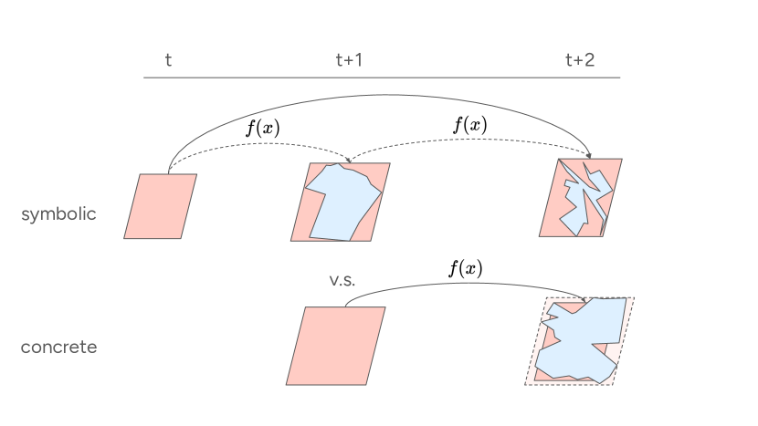
Figure 1: An illustration of overapproximate forward reachability. A symbolic query implicitly constrains the reachable set at intermediate timesteps producing tighter final sets. This concept is central to the refinement algorithm.

There have been many approaches in the reachability literature to address tractability and tightness. One of the central concepts used is domain refinement [3, 4]. Domain refinement refers to splitting the domain into subsets, e.g., through gridding, and computing the reachable set for each subset. Without domain refinement, the reachable set approximation would be unusably loose, but if gridded too finely the problem can become intractable as there is then exponential complexity in the number of state dimensions.

Another concept that has been used in the reachability literature is decomposition [5, 6, 7]. Decomposition refers to re-writing the system dynamics into a collection of uncoupled or loosely coupled subsystems. If e.g., using gridding to produce tight set approximations, fine gridding can then be used on each low dimensional subsystem without incurring the exponential cost of gridding the original high dimensional system.

Lastly, many methods make use of pre-specified template sets in order to speed up computation [8, 9, 10, 11]. In these methods, the tightest circumscribing (or inscribing) set of a particular type such as a hyperrectangle, ellipsoid, or zonotope is computed rather than computing the arbitrary non-convex true reachable set.

In this work we make use of a concept known as symbolic reachability [8] to define an algorithm for temporal refinement. Many verification methods use concrete reachability which involves computing the approximate reachable set at time $t+1$ using only the approximate reachable set at time $t$, or $t-1$ from $t$ in the backward case [12]. While concrete reachability is fast, it accumulates large approximation error quickly, a phenomenon known as the “wrapping effect” [13]. Symbolic reachability can be used to mitigate this effect [8]. Using symbolic reachability, the approximate reachable set at e.g., time $t+2$ is computed from the set at time $t$ while implicitly constraining the system trajectories to pass through the intermediate set at time $t+1$ (fig. 1). This results in tighter sets than if the set at $t+2$ was computed using only the approximate set at time $t+1$. It is possible to perform symbolic reachability for limited time horizons (temporal depths), each iteration computing a set farther into the future (or further in the past) and implicitly constraining system trajectories to pass through all sets at timesteps in between, but the problem will quickly approach intractability. To address this tradeoff between tightness and tractability, the authors of [8] perform hybrid-symbolic reachability which uses mixtures of concrete and symbolic computations in a hand-tuned, ad-hoc manner.

In this paper, we contribute a temporal refinement algorithm to automate hybrid-symbolic reachability analysis for tenuously tractable discrete-time dynamical systems. The temporal depth and end timestep of each query are automatically selected to produce tight reachable sets given the remaining computational budget and projected total computation length. Our algorithm is an orthogonal contribution to existing strategies for balancing tightness and tractability because it may be combined with concepts such as domain refinement, system decomposition, and pre-specified template sets; among others.

We demonstrate our algorithm for temporal refinement on overapproximate forward reachability analysis, but it is similarly applicable to backward reachability analysis and underapproximation. Specifically, we treat a challenging class of problems: computing forward reachable sets for discrete time nonlinear dynamical systems with neural network control policies; also called Neural Feedback Loops (NFLs). For this class of problem, there has been work on computing forward reachable sets [8], backward reachable sets [15], performing domain refinement [16, 4, 17], and using exotic template polyhedron [18] but there remains difficulty balancing tractability and tightness making it a good class of problem on which to demonstrate our technique. We use several examples from the literature and show that our approach can produce a range of overapproximation error values depending on the allotted computational budget, including computing reachable sets 20-70% faster than previous hand-tuned approaches for the same amount of error in the reachable set approximation.

2 Problem Definition

Consider a discrete time dynamical system with state $\vec{x}\in R^{d}$ governed by update equation $\vec{x}_{t+1}=f(\vec{x}_{t},\vec{u}_{t})$ with $\vec{u}\in R^{m}$. In this paper, we focus on nonlinear update functions $f$ but linear systems may also be considered. The control input $\vec{u}_{t}=c(\vec{x}_{t})$ comes from a feedback control policy.

We seek to compute the forward reachable sets $\mathcal{R}_{t}$ of the controlled system at future timesteps $t\in 1,2,3,\ldots$. The forward reachable set at time $t_{n}$, $n$ steps into the future from time $0$ is defined as follows:

$$\mathcal{R}_{n}\triangleq\{\vec{x}_{n}\mid\vec{x}_{n}=f(\vec{x}_{n-1},c(\vec{x}_{n-1})),$$ (1)

$$\vec{x}_{n-1}=f(\vec{x}_{n-2},c(\vec{x}_{n-2})),$$

$$\ldots,$$

$$\vec{x}_{1}=f(\vec{x}_{0},c(\vec{x}_{0})),$$

$$\vec{x}_{0}\in\mathcal{X}_{0}\}$$

where $\mathcal{X}_{0}$ is the initial set of states. As aforementioned, methods exist to compute the exact reachable set $\mathcal{R}_{t}$ for classes of linear or piecewise linear systems, but for arbitrary smooth nonlinear dynamics, approximation (over or under) must be used. In this paper we denote the overapproximate reachable set $\tilde{\mathcal{R}_{t}}$ where $\mathcal{R}_{t}\subseteq\tilde{\mathcal{R}_{t}}$. The overapproximation error $e$ at a given time $t$ is defined

$$e=\frac{m(\tilde{\mathcal{R}_{t}})}{m(\mathcal{R}_{t})}$$ (2)

where $m$ is an error metric and the desired value is $e=1$. The error over a finite time horizon $t\in\{1\ldots n\}$ is defined

$${e}=\frac{\sum_{t=1}^{n}m(\tilde{\mathcal{R}_{t}})}{\sum_{t=1}^{n}m({\mathcal{R}_{t}})}$$ (3)

Thus the problem this paper addresses may be stated as follows. When performing finite time hybrid-symbolic reachability analysis of $n$ steps for a discrete time dynamical system, algorithmically select points $t_{i}\in\{1,\ldots,n\}$ at which to perform symbolic reachability queries and select temporal depths $b_{\text{steps}}\in\{1\ldots t_{i}\}$ for those symbolic queries so as to minimize approximation error (eq. 3) while adhering to a pre-specified computational budget $b$.

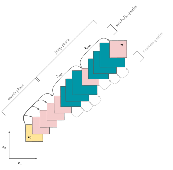
Figure 2: Symbolic reachability scheme for primary refinement. In this example $b_{\text{steps}}=4$.

3 Refinement Algorithm

At a high level, the algorithm begins in the “search” phase and searches for an estimate of the longest tractable temporal depth (symbolic horizon) $b_{\text{steps}}$. The algorithm then moves to a “jump” phase and performs symbolic queries of that temporal depth or shorter until the set at the desired final time $n$ has been reached. Alg. 1 provides more detail. In alg. 1, $\mathcal{X}_{0}$ is the initial set for reachability analysis, $b$ is the time budget in seconds, and $q$ is a query object consisting of a dynamics function $f$, a neural network controller $c(x):=NN(x)$, a final time horizon $n$, a variable to store current temporal depth $h$, and various parameters (e.g., hyperparameters controlling tightness of the nonlinear overapproximation). The method returns $\tilde{\mathbb{R}}$ a vector of reachable sets $\tilde{\mathcal{R}}_{t},\forall t\in[1\ldots n]$.

The motivation for the structure of the algorithm comes partially from the initial work on hybrid-symbolic reachability [8] which used long symbolic jumps with one-step concrete queries to generate the sets in between. Long symbolic jumps produce tight approximations of the reachable set and beginning symbolic jumps from tight approximations limits the wrapping effect. However, in this paper, a reasonable symbolic “jump” size is not known a priori so we first search for a long jump size. The search procedure also has the benefit of limiting reachable set growth. Small errors early in the time horizon compound over many timesteps, and because the search phase produces tight reachable sets for early steps, it limits error compounding.

Alg. 1 begins in the “search” phase with a temporal depth of $b_{\text{steps}}=1$ (line 3) beginning from the set $\mathcal{X}_{0}$ at time $t_{0}$ (lines 4-5). A symbolic reachability query is then performed (lines 7-8), and the new set(s) are then logged (lines 9-13). If there is enough time budget to continue searching, $b_{\text{steps}}$ will increment by $1$ (line 16). Symbolic reachable set computation queries are performed from the initial set $\mathcal{X}_{0}$ at time $t_{0}$ to increasingly large temporal depths / numbers of steps $b_{\text{steps}}$ into the future until it is estimated that trying a temporal depth one step longer would put the entire reachable set procedure over budget. Once this occurs, the algorithm will enter the “jump” phase and perform symbolic queries beginning from the set at $t_{\text{start}}:=t_{\text{cur}}$ (line 18-19) of temporal depth $b_{\text{steps}}$ or shorter until the set at the desired final time $n$ has been reached (line 6). Line 21 keeps $b_{\text{steps}}$ within correct range; and line 22 updates the early stopping timeout. The early stopping timeout limits budget overruns and is hand-tuned. The algorithm returns the reachable sets from time $t=1\ldots n$.

1 function RefinedReach($q$, $\mathcal{X}_{0}$, $b$):

2      

3      set_initial_timeout!($b$, $q$)

4       phase $\leftarrow$ “search”; $b_{\text{steps}}\leftarrow 1$

5       $t_{\text{start}}\leftarrow$ 0; $t_{\text{cur}}\leftarrow$ 0;

6       $\mathcal{X}_{\text{start}}\leftarrow\mathcal{X}_{0}$; $\tilde{\mathbb{R}}\leftarrow$ []

7       while $t_{\text{cur}}<n$ do

8             q.h $\leftarrow$ $b_{\text{steps}}$

9             data, $\tilde{\mathbb{R}}_{\text{out}}$ $\leftarrow$ symbolic_reach($q,\mathcal{X}_{\text{start}}$)

10             if phase == “search” then

11                   push!($\tilde{\mathbb{R}}$, $\tilde{\mathbb{R}}_{\text{out}}[end]$)

12            

13            else

14                   push!($\tilde{\mathbb{R}}$, $\tilde{\mathbb{R}}_{\text{out}}$)

15                  

16             end if

17            $t_{\text{cur}}\leftarrow t_{\text{start}}+b_{\text{steps}}$

18             $b\leftarrow b~{}-~{}$elapsed()

19             $b_{\text{steps}_{0}}$, phase $\leftarrow$ calc_steps($t_{\text{start}},b_{\text{steps}},b$, data, $t_{\text{est}}$, $n$, phase, status(q))

20             if phase == “jump” then

21                   $t_{\text{start}}\leftarrow t_{\text{start}}+b_{\text{steps}}$

22                   $\mathcal{X}_{\text{start}}\leftarrow\tilde{\mathbb{R}}[t_{\text{start}}$]

23                  

24             end if

25            $b_{\text{steps}}\leftarrow\min(b_{\text{steps}_{0}},n-t_{\text{start}})$

26             update_timeout!($q$, $b$)

27            

28       end while

29      return $\tilde{\mathbb{R}}$

30

Algorithm 1 Reachability for NFLs with automatic temporal refinement

One of the key pieces of Algorithm 1 lies within the subroutine calc_steps (line 16) which determines whether to continue searching for a longer temporal depth $b_{\text{steps}}$ or to move to the “jump” phase. The complete algorithm for calc_steps is included in the Appendix (alg. 2) and described here. calc_steps first estimates the amount of time needed compute one symbolic step, $t_{\text{est}}$, assuming that the time to compute a symbolic query of $m$ steps is roughly $t_{\text{est}}*m$. This is a simplification that is not strictly accurate – the time a symbolic query takes may be in the worst case exponential in temporal depth for some problems and timing depends on the particular input set – but it leads to roughly accurate budgeting given that $t_{\text{est}}$ is updated at each iteration. The algorithm then estimates the time that future queries will take and uses this to determine if there is enough time budget to continue searching. This time estimate includes a symbolic query from $t_{0}$ to $b_{\text{steps}}+1$ plus the time to finish finish the temporal horizon in the “jump” phase. If the remaining budget $b$ is large enough, the algorithm increments $b_{\text{steps}}\leftarrow b_{\text{steps}}+1$ and if not, the algorithm enters the “jump” phase. Finally, if the solver stops early, the phase is also switched to “jump”. The early stopping is used to ensure the budget is approximately respected given that the estimated time per symbolic step $t_{\text{est}}$ is not an upper bound.

Note that long symbolic queries generally produce tight reachable sets but shorter queries can produce tighter sets if the starting set of the shorter query is tighter itself.

4 Overapproximate Forward Reachability

Our refinement algorithm is applicable to both forwards and backwards reachability and both over (outer) and under (inner) approximation but in this paper, we demonstrate our refinement algorithm on overapproximate forward reachability of nonlinear neural feedback loops (NFLs). In particular, we use the reachability approach presented in [8]. To briefly summarize, the approach computes tight piecewise linear bounds for smooth nonlinear functions in the dynamics and then encodes these bounds as well as the ReLU neural network control policy into a mixed integer linear program. A hyperrectangular template set is then optimized to obtain an overapproximation of the reachable set. The mixture of symbolic and concrete queries is determined by the refinement algorithm presented here, but the procedure to approximate nonlinear functions and compute approximate reachable sets using mixed integer programs comes from [8] where further details can be found.

5 Soundness, Completeness, Complexity

The algorithm is sound, i.e. $\mathcal{R}_{t}\subseteq\tilde{\mathcal{R}}_{t}$, for all $t$, following directly from the soundness of [8]. In terms of completeness, the algorithm presented here does not guarantee that the overapproximate reachable sets $\tilde{\mathcal{R}}_{t}$ converge to the true reachable sets $\mathcal{R}_{t}$. The method presented here could in theory be combined with methods that provably converge to the true reachable set for some classes of nonlinear systems [19] to overcome this limitation, but completeness in this sense is beyond the scope of this paper.

The algorithm is guaranteed to produce a sequence of reachable sets as even with early stopping, the algorithm will extend the compute time until a finite feasible solution with $<50\%$ relative duality gap has been found. The algorithm is guaranteed to terminate under the mild assumption that a feasible solution with $<50\%$ relative duality gap exists.

The time complexity of this algorithm is in the worst case NP-hard as it involves solving mixed integer linear programs. However, the average case complexity is in practice more reasonable as is demonstrated in the results section.

6 Numerical Experiments

Numerical experiments were run on examples taken from  [8, 20] to assess the tightness and computational speed of the temporal refinement algorithm. Four problems were used: the pendulum dynamical system with a controller of 2 layers, 25 neurons per layer (S1); the TORA dynamical system with a controller of 3 layers, 25 neurons per layer (T1); the car dynamical system with a controller of 1 layer with 100 neurons (C1) and a controller of 1 layer with 200 neurons (C2). The reader is referred to [8] for the details on the neural network controlled dynamical systems.

6.1 Results

The temporal refinement algorithm was run multiple times to assess how changing the time budget changes the approximate reachable set error. Figure 3 measures the approximation error of the sets computed by the optimizer using the ratio of the sum of volumes:

$$e_{\text{total}}=\frac{\sum_{t=1}^{n}\text{vol}(\tilde{\mathcal{R}}_{t})}{\sum_{t=1}^{n}\text{vol}(\text{\@text@baccent{$\mathcal{R}_t$}})}$$ (4)

In fig. 3, one can observe that the approximate error generally decreases with increasing budget. Note that the trend is not monotonic because the algorithm is a heuristic.

We compare our algorithm to the hand tuned hybrid symbolic approach used in [8] which is represented in  fig. 3 as dotted lines. One might expect that the hand tuned approach would produce approximate reachable sets more quickly for a given amount of error. A significant amount of work was presumably done offline to identify good symbolic intervals that must instead be identified at runtime with our approach. However, it turns out that our heuristic can actually produce approximate reachable sets with similar amounts of error as the hand-tuned approach in 20-70% less time, as shown in fig. 3. Furthermore, our approach is able to produce reachable sets for some problems such as the pendulum problem S1 that have 40% less error than the hand-tuned approach when allowed to compute for longer than the time taken by the hand-tuned approach.

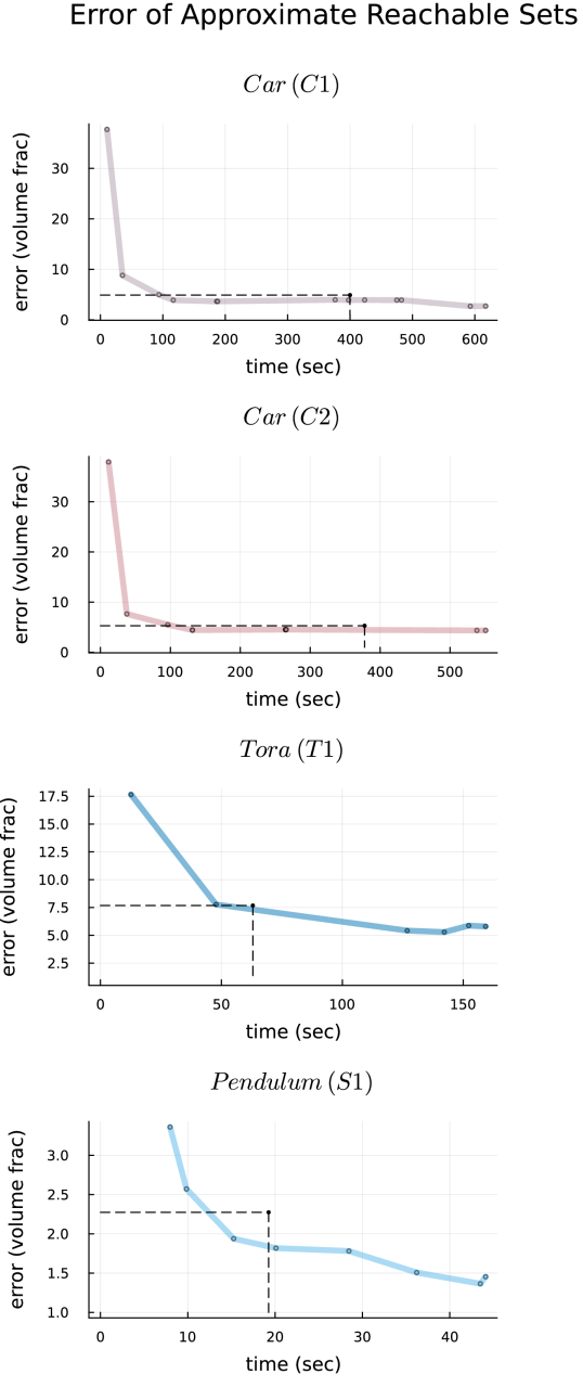
Figure 3: Approximate reachable sets of various fidelity are produced depending on allotted time and are competitive with hand-tuned baseline indicated with dashed lines.

We also compare sets produced by our algorithm to concrete one step reachable sets. Using one step sets is fast but leads to large approximation error. Examples of the reachable sets computed by our algorithm and baselines can be seen in  fig. 4 and fig. 5. Set are compared both using eq. 4 as well as the ratio of the sum of radii:

$$e_{\text{total}}=\frac{\sum_{t=1}^{n}\big{(}\sum_{i=1}^{d}\text{radius}_{i}(\tilde{\mathcal{R}}_{t})\big{)}}{\sum_{t=1}^{n}\big{(}\sum_{i=1}^{d}\text{radius}_{i}(\text{\@text@baccent{$\mathcal{R}_t$}})\big{)}}$$ (5)

One step concrete sets are labeled ’naive’ and one can observe that every set produced by our approach is equal to or tighter than those produced with the naive approach. To compare to the hand-tuned approach, we select a run from fig. 3 that had roughly equivalent or less error in a smaller amount of time and calculate the increase in speed by our approach. For the runs selected in fig. 4 and fig. 5, not every set produced by our approach is tighter than sets produced by the hand tuned approach, but when error is calculated over all sets in the trajectory, the total error is roughly equal or smaller. For pendulum problem S1 featured fig. 4, our algorithm is 20.9% faster than the hand-tuned approach for less error by both radius and volume metrics, and for the TORA problem T1 featured in fig. 5, our algorithm is 24% faster for an $\approx$ equal amount of error (1.5% less error according to the ratio metric and 1.2% more error according to the volume metric).

In fig. 6, we display numerical results for the remaining problems, car problems C1 and C2. For C1 and C2, we select runs that have less error by both radius and volume metrics and are respectively 70.8% faster and 65.2% faster, which translates to 4.7 minutes faster and 4.1 minutes faster.

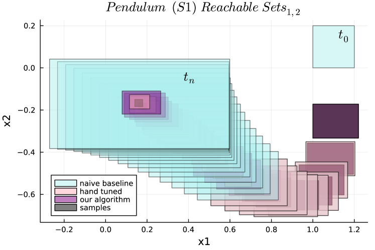
	Naive	Hand-Tuned	Ours
Error (volume)	11.9	2.27	1.94
Error (radius)	3.79	1.61	1.59
Time	7.84s	19.3s	15.3s

Figure 4: Reachable sets for pendulum problem S1 with two layer, 25 neuron-per-layer neural network controller show less error than the naive baseline and greater speed than the hand-tuned baseline for less error.

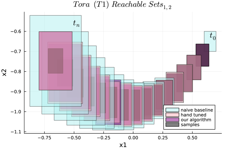
	Naive	Hand-Tuned	Ours
Error (volume)	31.7	7.67	7.78
Error (radius)	1.81	1.41	1.38
Time	6.62s	63.0s	47.8s

Figure 5: Dimensions 1 and 2 of the reachable sets for TORA problem T1 with three layer, 25 neuron-per-layer neural network controller which has less error than the naive baseline and greater speed than the hand-tuned baseline for similar error.

Car (C1)	One-Step	Hand-Tuned	Ours
Error (volume)	37.7	4.90	3.89
Error (radius)	1.88	1.31	1.28
Time	10.3s	400s	117s
Car (C2)
Error (volume)	37.9	5.29	4.43
Error (radius)	1.85	1.30	1.29
Time	11.1s	378s	131s

Figure 6: Reachable sets for the Car problems C1 and C2 are computed significantly faster for comparable error using our algorithm as compared to the hand-tuned baseline.

Lastly, our code will be released as an open source tool and be available here.

6.2 Limitations

The approach described here has limitations related to budgeting. A poor choice of initial solution from optimizer can lead to budget overruns as the algorithm will continue to compute if a finite solution has not yet been found. Further, budgeting with the linear time approximation as described is not accurate for all reachability problems, leading to budget overruns and/or conservative solutions for some problems; which may be exacerbated by long horizon queries. As previously mentioned, our algorithm is a heuristic. There does not exist a guarantee that given two budgets $b_{A}>b_{B}$ the sets produced with budget $b_{A}$ will be tighter than those produced using $b_{B}$.

7 Conclusion

In this paper we have introduced an algorithm for temporal refinement of tenuously tractable discrete time reachability problems. The algorithm computes reachable sets using constraints from several timesteps at once in order to produce tighter sets. The temporal depth of timestep constraints considered for a given reachable set is calculated based upon remaining computational budget and estimated future computation. The algorithm introduced here makes it possible to do hybrid-symbolic reachability without hand tuning concrete and symbolic intervals. We demonstrated this algorithm on a difficult class of reachability problems: nonlinear dynamical systems with neural network control policies, and demonstrated that it is able to produce reachable sets of varying error given varying computational budget. Additionally, it is able to produce reachable sets 20-70% faster then hand tuned approaches for the same amount of error. Ultimately, this algorithm and associated open-source code represent tools to enable more efficient reachability analysis for complex control systems.

.1 Calculating temporal depth for Algorithm  LABEL:alg:initial_reach

Algorithm 2, calc_steps, calculates the next symbolic query for alg. 1. In line 2 of alg. 2, calc_steps calculates the time index of the current step, $t_{\text{cur}}$, and then in line 3, calc_steps makes a conservative estimate of the amount of time needed compute one symbolic step, $t_{\text{est}}$. If previously, phase = “search”, (line 4), and we have not stopped early (line 5), we will estimate if there is enough time budget to continue searching (line 6).

To estimate if there is enough time budget to continue searching, we must estimate the time that future symbolic queries will take. Assuming that the time it takes to perform 1 symbolic step is roughly constant ($t_{\text{est}}$) and that we are in the search phase, the last symbolic query was from step 0 of length $b_{\text{steps}}$, and the time cost of a potential next query from time 0 to time $b_{\text{steps}}+1$ is $\approx t_{\text{est}}*(b_{\text{steps}}+1)$. At any given time, the total remaining computational cost of primary_refinement is the cost of the next search step plus the cost of symbolic jumps to finish the time horizon in the “jump” phase which can be estimated as taking time $(n-(t_{\text{cur}}+1))*t_{\text{est}}$. As $t_{\text{cur}}=b_{\text{steps}}$ during the search phase, the total time estimate for one further symbolic query from $0$ to $b_{\text{steps}}+1$ plus jumps from $b_{\text{steps}}+1$ to $n$ is then $t_{\text{est}}*(b_{\text{steps}}+1)+(n-(b_{\text{steps}}+1))*t_{\text{est}}=n*t_{\text{est}}$ (see line 6).

This estimate assumes that the time to compute $m$ symbolic steps is roughly $t_{\text{est}}*m$ regardless of whether those steps are computed in 2 symbolic queries of size $\frac{t_{\text{est}}*m}{2}$ or 10 symbolic queries of size $\frac{t_{\text{est}}*m}{10}$. This is a simplification we make that is not strictly accurate – the time a symbolic query takes may be exponential in temporal depth for some problems and timing depends on the particular input set – but it leads to roughly accurate budgeting given that $t_{\text{est}}$ is updated at each iteration.

If the remaining budget $b$ does allow for continued search, $b_{\text{steps}}$ is incremented (alg. 2 line 7). If not, we instead calculate a reasonable temporal query depth for finishing the remaining steps of the reachability problem in the jump phase (lines 8-13). One could use jumps of size $b_{\text{steps}}$ but if $n$ is not divisible or close to divisible by $b_{\text{steps}}$ this could lead to a short jump at the end of the horizon and a loose final set. Instead, we calculate the num_jumps needed to finish the time horizon in jumps of size $b_{\text{steps}}$ (line 9-10) and instead use jumps of size $\text{ceil}(\frac{s_{\text{left}}}{\text{num\_jumps}})$ (line 11) which makes all the jumps closer in size.

If the solver has stopped early (line 14), the phase is switched to “jump” (line 18) and a similar calculation is performed to estimate the jump size (lines 15-17) with the difference being num_jumps is calculated using $b_{\text{steps}}-1$ instead of $b_{\text{steps}}$ (line 16). If we are already in the “jump” phase (line 20) we do not change the jump size of $b_{\text{steps}}$ unless we stop early (line 21) in which case we decrement $b_{\text{steps}}$ by 1 (line 22). The early stopping is used to ensure the budget is approximately respected given that the estimated time per symbolic step $t_{\text{est}}$ is not an upper bound.

1 function calc_steps($t_{\text{start}},b_{\text{steps}},b$, data, $n$, phase, status):

2       $t_{\text{cur}}\leftarrow t_{\text{start}}+b_{\text{steps}}$

3      $t_{\text{est}}\leftarrow\max(t_{\text{est}},\text{data}[t_{\text{cur}}].\text{time}/\text{data}[t_{\text{cur}}].\text{steps})$

4      if phase == “search” then

5             if status == “nominal” then

6                   if $n*t_{\text{est}}<b$ then

7                         $b_{\text{steps}}\leftarrow b_{\text{steps}}+1$

8                        

9                   else

10                         $s_{\text{left}}\leftarrow n-b_{\text{steps}}$

11                         num_jumps = $\text{ceil}(\frac{s_{\text{left}}}{b_{\text{steps}}})$

12                         $b_{\text{steps}}\leftarrow\text{ceil}(\frac{s_{\text{left}}}{\text{num\_jumps}})$

13                         phase $\leftarrow$ “jump”

14                   end if

15                  

16            else if status == “stopped early” then

17                   $s_{\text{left}}\leftarrow n-b_{\text{steps}}$

18                   num_jumps = $\text{ceil}(\frac{s_{\text{left}}}{b_{\text{steps}}-1})$

19                   $b_{\text{steps}}\leftarrow\text{ceil}(\frac{s_{\text{left}}}{\text{num\_jumps}})$

20                   phase $\leftarrow$ “jump”

21             end if

22            

23       else if phase == “jump” then

24             if status == “stopped early” then

25                   $b_{\text{steps}}=\max(b_{\text{steps}}-1,1)$

26             end if

27            

28       end if

29      return $b_{\text{steps}}$, phase

30

Algorithm 2 Procedure to calculate symbolic steps during primary refinement.

References

- [1] G. Frehse, C. Le Guernic, A. Donzé, S. Cotton, R. Ray, O. Lebeltel, R. Ripado, A. Girard, T. Dang, and O. Maler, “Spaceex: Scalable verification of hybrid systems,” in Computer Aided Verification: 23rd International Conference, CAV 2011, Snowbird, UT, USA, July 14-20, 2011. Proceedings 23. Springer, 2011, pp. 379–395.
- [2] J.-J. E. Slotine, “Applied nonlinear control,” PRENTICE-HALL google schola, vol. 2, pp. 1123–1131, 1991.
- [3] S. Bansal, M. Chen, S. Herbert, and C. J. Tomlin, “Hamilton-jacobi reachability: A brief overview and recent advances,” in 2017 IEEE 56th Annual Conference on Decision and Control (CDC). IEEE, 2017, pp. 2242–2253.
- [4] M. Everett, R. Bunel, and S. Omidshafiei, “Drip: domain refinement iteration with polytopes for backward reachability analysis of neural feedback loops,” IEEE Control Systems Letters, 2023.
- [5] M. Chen, S. L. Herbert, M. S. Vashishtha, S. Bansal, and C. J. Tomlin, “Decomposition of reachable sets and tubes for a class of nonlinear systems,” IEEE Transactions on Automatic Control, vol. 63, no. 11, pp. 3675–3688, 2018.
- [6] I. M. Mitchell and C. J. Tomlin, “Overapproximating reachable sets by hamilton-jacobi projections,” journal of Scientific Computing, vol. 19, pp. 323–346, 2003.
- [7] X. Chen and S. Sankaranarayanan, “Decomposed reachability analysis for nonlinear systems,” in 2016 IEEE Real-Time Systems Symposium (RTSS). IEEE, 2016, pp. 13–24.
- [8] C. Sidrane, A. Maleki, A. Irfan, and M. J. Kochenderfer, “OVERT: An algorithm for safety verification of neural network control policies for nonlinear systems,” The Journal of Machine Learning Research, vol. 23, no. 1, pp. 5090–5134, 2022.
- [9] A. B. Kurzhanski and P. Varaiya, “Ellipsoidal techniques for reachability analysis: internal approximation,” Systems & control letters, vol. 41, no. 3, pp. 201–211, 2000.
- [10] W. Kühn, “Rigorously computed orbits of dynamical systems without the wrapping effect,” Computing, vol. 61, pp. 47–67, 1998.
- [11] M. Althoff and B. H. Krogh, “Zonotope bundles for the efficient computation of reachable sets,” in 2011 50th IEEE conference on decision and control and European control conference. IEEE, 2011, pp. 6814–6821.
- [12] J. A. Siefert, T. J. Bird, J. P. Koeln, N. Jain, and H. C. Pangborn, “Successor sets of discrete-time nonlinear systems using hybrid zonotopes,” in 2023 American Control Conference (ACC). IEEE, 2023, pp. 1383–1389.
- [13] A. Neumaier, The wrapping effect, ellipsoid arithmetic, stability and confidence regions. Springer, 1993.
- [14] M. Wetzlinger, A. Kulmburg, A. Le Penven, and M. Althoff, “Adaptive reachability algorithms for nonlinear systems using abstraction error analysis,” Nonlinear Analysis: Hybrid Systems, vol. 46, p. 101252, 2022.
- [15] N. Rober, S. M. Katz, C. Sidrane, E. Yel, M. Everett, M. J. Kochenderfer, and J. P. How, “Backward reachability analysis of neural feedback loops: Techniques for linear and nonlinear systems,” IEEE Open Journal of Control Systems, 2023.
- [16] N. Rober, M. Everett, S. Zhang, and J. P. How, “A hybrid partitioning strategy for backward reachability of neural feedback loops,” in 2023 American Control Conference (ACC). IEEE, 2023, pp. 3523–3528.
- [17] W. Xiang, H.-D. Tran, X. Yang, and T. T. Johnson, “Reachable set estimation for neural network control systems: A simulation-guided approach,” IEEE Transactions on Neural Networks and Learning Systems, vol. 32, no. 5, pp. 1821–1830, 2020.
- [18] D. Manzanas Lopez, T. Johnson, H.-D. Tran, S. Bak, X. Chen, and K. L. Hobbs, “Verification of neural network compression of acas xu lookup tables with star set reachability,” in AIAA Scitech 2021 Forum, 2021, p. 0995.
- [19] E. Asarin, T. Dang, and A. Girard, “Reachability analysis of nonlinear systems using conservative approximation,” in International Workshop on Hybrid Systems: Computation and Control. Springer, 2003, pp. 20–35.
- [20] T. Johnson, D. Lopez, P. Musau, H. Tran, T. Botoeva, F. Leofante, A. Maleki, C. Sidrane, J. Fan, and C. Huang, “Arch-comp20 category report: Artificial intelligence and neural network control systems (AINNCS) for continuous and hybrid systems plants,” EPiC Series in Computing, vol. 74, pp. 107–139, 2020.