New simple and accurate approximations for quintessence
Abstract
We derive new simple approximations for quintessence in a spatially homogeneous, isotropic and flat spacetime. The approximations are typically an order of magnitude more accurate than anything available in the literature, which from an observational perspective makes numerical calculations superfluous. For example, our tracking quintessence approximation, with one less parameter than CPL and a comparably simple expression, yields a maximum relative error of for the inverse power law scalar field potential. We situate the new results in a broader dark energy context, where the present parametrized deviations from CDM offer simple alternatives to the CPL parametrization, useful for observations at increasingly large redshifts.
1 Introduction
A growing number of increasingly precise cosmological observations of, e.g., type Ia supernovae [1, 2, 3], the cosmic microwave background (CMB) [4], various measurements of the Hubble parameter [5, 6, 7], the universe large-scale structure (LSS) [8, 9], and baryon acoustic oscillations (BAO) [10, 11, 12, 13], suggests that the universe is presently accelerating. In addition cosmological observations indicate that most of the matter in the universe is invisible ‘dark matter’ [14, 15, 16, 17]. The standard interpretation of the observations rely on that General Relativity is an accurate description of gravity on cosmological scales and that the observable Universe is almost spatially homogeneous, isotropic and flat on sufficiently large spatial scales. This leads to that the acceleration of the universe requires a ‘dark energy’ (DE) density component, , with sufficiently large negative pressure, while the dark matter seems to be best described by a dominant cold dark matter (CDM) energy density component, , without pressure. The most simple and remarkably successful model that is compatible with these assumptions is the CDM model, for which the energy density and pressure are given by , where is the cosmological constant.
There are, however, theoretical problems, e.g., the nature of dark matter [18, 19], the observed small value of , the coincidence problem, see e.g. [20] and references therein. Recent tensions between some data sets [21, 22, 23] and that large scale structures seem to form surprisingly early in the universe [24] have further aggravated the situation, which has contributed as motivation for numerous dynamical DE models for which is evolving. Many of these models are purely cosmographically motivated, without any tie to any theory, notably the Chevallier-Polarski-Linder (CPL) parametrization [25, 26] of the DE equation of state parameter and a plethora of variations of it, see e.g. [27] and references therein.
Some DE models, however, endeavour to have some theoretical motivation, where one of the simplest attempts is quintessence, i.e. a canonical scalar field, , that is minimally coupled to gravity, see e.g. [28] and [29] for references. This is the main topic of the present paper, which deals with a non-interacting scalar field and matter in a spatially homogeneous, isotropic and flat spacetime, although we note that the ideas in this paper are applicable to many other models and alternative theories. More specifically, we will derive simple and accurate approximations for thawing and tracking quintessence,111According to Tsujikawa (2013) [28] there are three types of quintessence in the literature: thawing, tracking and scaling freezing quintessence, see [30] for subtleties. In this paper we consider tracking quintessence for asymptotically inverse power law scalar field potentials , , when . Since scaling freezing quintessence does not yield past continuous deformations of CDM we will only briefly touch on this topic in appendix B. which yield continuous deformations of CDM cosmology.
The outline of the paper is as follows. Motivated by our new quintessence approximations, the next section provides a general DE context. In Section 3 we derive the expressions for the parameters appearing in the previous DE section for thawing and tracking quintessence. The new thawing and tracking quintessence approximations are compared with numerical calculations and previous results in the literature in section 4. The main part of the paper ends with section 5, which includes suggestions for future applications of the present approach and results. Appendix A reviews quintessence approximations found in the literature, while appendix B deals with scaling freezing quintessence.
2 Dark energy considerations
2.1 Preliminaries
Spatially homogeneous, isotropic and flat spacetimes have a line element that can be written as222We use units such that and , where is the speed of light and is the gravitational constant.
| (1) |
where is the cosmological scale factor, (throughout, a subscript 0 refers to quantities at the present time ), where is usually set to one by an appropriate scaling of the spatial coordinates;
| (2) |
denotes the Hubble parameter, where the dot refers to differentiation with respect to the cosmic time , while is the redshift.
Since the spacetime is described by the Hubble parameter it follows that cosmological observables and their interpretation depend directly on , its derivatives and integrals. This is illustrated by, e.g., the deceleration parameter , and many distance measures, e.g., the Hubble distance , the proper motion or coordinate distance , the luminosity distance , the angular diameter distance , which are given by (see, e.g. [27])
| (3a) | ||||
| (3b) | ||||
| (3c) | ||||
| (3d) | ||||
To find interesting alternatives to CDM some authors simply choose some , e.g. being a polynomial in as in [27], or obtain by assuming a specific form for one of the distance measures, e.g. , which yield via , see e.g. [27]. More commonly, however, is to make a choice of the DE equation of state parameter that is different than the CDM value (see e.g. [23] and references therein for a plethora of examples of and ). Note, however, that is not a physical observable. Since cosmological observations depend on , it is necessary to compute from , which requires the Einstein field equations and the matter conservation equations.
Although the distance measures are naturally expressed in terms of the redshift , computations are usually simpler using the -fold time , where it is subsequently trivial to transform results to the redshift by using the relation
| (4) |
For simplicity we consider only non-interacting pressure free matter and a dark energy component.333Although the gravitational influence of radiation is negligible when quintessence is important for the evolution of the Universe, we will comment on how to add it to our approximations in section 5. The matter conservation equations for the matter energy density, and the DE energy density, , are given by
| (5a) | ||||||||
| (5b) | ||||||||
where a ′ denotes the derivative with respect to and where is defined as
| (6) |
2.2 Relationships between , , and
Next we introduce the dimensionless and bounded Hubble normalized variables , and the dimensionless DE equation of state parameter :
| (7) |
where we have used the Friedmann equation (i.e. the Gauss constraint)
| (8) |
which yields444To improve our approximations we will use , but subsequently the relation can be used to bring the approximations closer to present day data.
| (9) |
To display the relationship between these quantities and it is convenient to introduce the present time normalized Hubble parameter
| (10) |
Equations (8), (5) and (7) result in the following DE expression for :
| (11) |
| (12) |
Since the above expressions involve , the integral (6) needs to be computed from .
We finally note that the deceleration parameter is defined as
| (14) |
and is related to the total equation of state parameter according to
| (15) |
where
| (16) |
To derive the above relations, we have used the Friedmann equation to obtain the last equality in (16), and also (14) and (5) to establish , which also follows from the Einstein field equations.
In the following sections we will discuss quintessence for which . As shown in section 3, see also e.g. [30] and [31], thawing quintessence yields while tracking quintessence leads to , . As a consequence thawing and tracking quintessence are asymptotically toward the past described by the CDM and CDM models, respectively. Let us therefore recall the properties of these models.
2.3 The CDM and CDM models
2.4 Past DE series expansions
Thawing and tracking quintessence, as illustrated in a dynamical systems setting in [30] and [31], are associated with attractor solutions that originate from fixed points on the matter dominant boundary where and . Treating both cases simultaneously as dark energy models, i.e., by letting and when , leads to that equation (13a), which can be written as , results in the approximation in this limit and hence
| (19) |
which is indeed the case for the quintessence models. To improve the approximation we now perform series expansions in
| (20) |
where when .
For brevity we only consider and . If one starts with a series expansion in and uses (6) and (12) one obtain an expression for that subsequently can be series expanded in ; on the other hand, if one starts with a series expansion in and inserts this into (13a) one obtains an expression for that one then can series expand in . These two procedures result in the same series expansions, which can be written as555The given expressions can be generalized by writing , which subsequently can be used to compute the series expansions for and, e.g., . The reason we have written as and as is that this simplifies and is compatible with our thawing and tracking quintessence approximations, where these use the Padé expression for in order to connect our approximations to the present time.
| (21a) | ||||
| (21b) | ||||
2.5 DE Padé approximants
For brevity we will restrict our considerations by following the most common approach in the literature, which is to use as the starting point. The series expansions provide approximations when is small, i.e. close to the matter dominated regime. To obtain approximations that are accurate even up to the present time we will use Padé approximants for the series expansion of in . Our first and second order expansions in for yield the following Padé approximants for :
| (22a) | ||||
| (22b) | ||||
To connect with the present time we can set and solve for in (22) in terms of the left hand side . However, since is not an observable we will instead relate to and thereby obtain a direct connection to the observables and since . To obtain accurate approximations at the present time for we consider the Padé approximant
| (23) |
from which it follows that , which yields
| (24) |
This is then inserted into (22a), which when used in (6) to obtain leads to the same expression as (23) with (24) inserted. To obtain a better approximation for one can then go on to Padé approximants also involving in the expansion.666These are given by and . To express in terms of obtained in this manner requires solving quadratic equations in , which leads to rather messy expressions. The approximation (23) turns out to be a fairly good approximations for quintessence. For this reason we will use the simple result in (24) also for in (22b). This leads to expressions for that can be written as follows:777Note that one can use the series expansion in for to obtain the following expression for : and use (24) for . This expression can subsequently be used to obtain various Padé approximants to obtain good quintessence approximations for and then use to compute, e.g., , if one is so inclined.
| (25a) | ||||
| (25b) | ||||
which lead to the following present time values
| (26a) | ||||
| (26b) | ||||
Note that setting in yields and that setting in both and results in , i.e., leads to the CDM model when and the CDM model when .
Inserting the expressions for and in (22) and (25) into (6) yields
| (27a) | ||||
| (27b) | ||||
where the first comes from and the second from .
It follows from (12) and (11) that the Padé approximant results in
| (28a) | ||||
| (28b) | ||||
where we recall that , , while the result for the Padé is obtained from the above expressions by setting , which yields888Note that by multiplying (29a) with it is easy to see that the transformation and yields the expression in (18a), which specializes to CDM when . In particular this leads to , which illustrates the danger of interpreting and transferring data from a CDM or CDM context to a different DE context.
| (29a) | ||||
| (29b) | ||||
It is trivial to express the above relations in the redshift , which is done explicitly in section 4 where we investigate the accuracy of thawing and tracking quintessence approximations. To do so, we need and , which we derive in the next section, but before doing this let us briefly consider the CPL parametrization.
2.6 The Chevallier-Polarski-Linder parametrization
The so-called CPL parameters [25, 26] are often used in cosmology and parameterize according to
| (30) |
where
| (31) |
By using that we can easily compute the parameter from (25):
| (32a) | ||||
| (32b) | ||||
Inserting (30) into (6) yields
| (33) |
which results in that (12) and (11) yield
| (34a) | ||||
| (34b) | ||||
and thereby
| (35a) | ||||
| (35b) | ||||
One can regard (30) as a series expansion in , but this is inconsistent with the past matter dominant requirement and that one of the CPL parameters can be interpreted as , since this naturally leads to an expansion in , which is particularly pertinent as observations probe increasingly large redshift. CPL thus mixes this asymptotically motivated function (arising from the part in (30)) in and with another function that comes from the part in (30). Due to this mixture of functions, especially the exponential part involving , the CPL parametrization arguably does not lead to simpler observables than our and based results, and it certainly is not a good approximation for thawing and tracking quintessence.
3 Deriving the parameters and for quintessence
3.1 Thawing quintessence
To obtain a system that is useful for deriving expressions for and for thawing quintessence999The concepts of thawing and freezing were defined by Caldwell and Linder (2005) [32] as follows: thawing is characterized by where subsequently grows, i.e. , while and holds for freezing. we introduce the following dimensionless bounded variable101010The variable was first introduced by Coley et al. (1997) [33] and Copeland et al. (1998) [34] whose is . Since then, (or ) is commonly used to describe scalar fields in cosmology, see, e.g., Urena-Lopez (2012) [35], equation (2.3), Tsujikawa (2013) [28], equation (16) and Alho and Uggla (2015) [36], equation (8). The reason for using the notation for the kernel is because plays a similar role as Hubble-normalized shear, which is typically denoted with the kernel , see e.g. [37].
| (36) |
and use as the state vector together with the -fold time .111111The variables and in [30] yield slower convergence. To obtain a dynamical system for we use that (13a) is equivalent to , , and that is given by
| (37) |
as follows from the definitions. In addition, the (non-linear) Klein-Gordon equation , expressed in -fold time, is needed. This leads to the dynamical system
| (38a) | ||||
| (38b) | ||||
| (38c) | ||||
where we have introduced
| (39) |
Since thawing quintessence begins in the matter dominated regime, , when initially, it follows from (37) and from that thawing quintessence begins when . We then note that whenever is bounded, which always holds for some domain of for any scalar field potential , there is a line of matter dominated ‘Friedmann-Lemaître’ fixed points given by
| (40) |
and hence , parameterized by the constant values . To determine what happens in the vicinity of we linearize the equations at , which leads to
| (41a) | ||||
| (41b) | ||||
| (41c) | ||||
where . It follows that thawing quintessence is associated with the unstable manifold of , obtained by setting . More precisely, thawing quintessence models consist of the 1-parameter set of unstable manifold orbits (i.e., solution trajectories) of and the open set of orbits that intermediately shadow these orbits; this open set of orbits consists of the orbits that before the thawing epoch are pushed toward by the stable manifold orbits of and subsequently toward the unstable manifold orbits of , which therefore approximate these orbits during their thawing stage of evolution, for details, see [30] and [38].
To find and we Taylor expand around and make a series expansion in for the variables . The coefficients in the expansion are found by inserting the expansions into the dynamical system (38) and solving for them. Truncation of the series in gives
| (42a) | ||||
| (42b) | ||||
| (42c) | ||||
where and are related to the slow-roll parameters
| (43) |
computed at on , i.e.,
| (44) |
according to
| (45) |
where a comparison between (21b) and (42c) results in
| (46) |
3.2 Tracking quintessence
Peebles and Ratra (1988) [39, 40] initiated the study of the inverse power law potential , . They obtained approximate expressions by assuming that and could be approximated by their values in the matter dominated regime and that the scale factor obeyed a power law dependence in cosmic time . Subsequently Ratra and Quillen (1992) [41] obtained the asymptotic result (their eq. (5)) for this potential. This work was then followed up by Zlatev et al. (1999) [42] and Steinhardt et al. (1999) [43],121212See also Podario and Ratra (2000) [44] and Peebles and Ratra (2003) [20]. who introduced the notation ‘tracker field’ as a form of quintessence, associated with potentials for which when and the condition , see also [28], where
| (47) |
We are here considering asymptotically inverse power law potentials, characterized by
| (48) |
Next, we introduce a dynamical system that is suitable for deriving approximations for the evolution in the vicinity of and as long the potential and are monotonically decreasing, i.e., when and , as follows from (39) and (47). The system of equations are based on the following new variables:131313The variables and are slightly different than the variables and in [31], which were adapted to a global state space setting, while the present ones are designed for fast convergence for the tracker orbit and the explicit appearance of in the equations and results.
| (49) |
from which it follows, when taken together with (37),
| (50) |
These variables lead to the dynamical system
| (51a) | ||||
| (51b) | ||||
| (51c) | ||||
where we assume that is regular in .
The dynamical system (51) admits (and thereby ) as an invariant boundary subset. As shown in [31], tracking quintessence is associated with a tracker orbit that originates from a tracker fixed point, , on the boundary, which in the present variables is given by
| (52) |
Notably is a hyperbolic saddle with the ‘tracker orbit’ as its unstable manifold and being its 2D stable manifold, which results in that the tracker orbit acts as an ‘attractor orbit’, see [31] for details.
To find the parameters , and we first note that the tracker fixed point value for gives the initial asymptotic tracker value for since
| (53) |
where describes the single positive eigenvalue, given by . Next we proceed and make a series expansion in
| (54) |
for the variables . Since the governing equations (51) involve we need to use a truncated Taylor series of at :
| (55) |
where .
To identify and we solve for the coefficients for the series expanded variables by using the equations in (51), which when inserted into yields with
| (56a) | ||||
| (56b) | ||||
| (56c) | ||||
| (56d) | ||||
where we in the expression for assume that . Note that the special class of models with , i.e. , needs special treatment and that it include models with , see [31] for details.141414Sahni and Starobinsky (2000) [45], equation (121), and Urena-Lopez and Matos (2000) [46], investigated models with the potential and showed that these models admit a special solution (which turns out to be the tracker orbit) for which is constant, i.e., they yield CDM spacetimes with .
4 Numerical comparisons
In this section we calculate numerical relative errors, i.e.,
| (57) |
of our approximations for thawing and tracking quintessence, but also for approximations found in the literature, described in appendix A. For brevity we will consider the relative errors of , and .
Before doing so, let us write our approximations for , , from which follows since , and in the redshift . The approximations based on and only involving are given by (as follows from (25a), (29a) and (29b)):
| (58a) | ||||
| (58b) | ||||
| (58c) | ||||
while the approximations obtained from , involving both and , are as follows:
| (59a) | ||||
| (59b) | ||||
| (59c) | ||||
| where | ||||
| (59d) | ||||
The parameters and for thawing quintessence were given in equations (45) and (46), while those for tracking quintessence are found in equations (56), where we recall that in the tracking quintessence case where . We cannot of course test all possible scalar field models, but we have done so for several potentials and obtained similar results. For brevity we will here only present the results for two scalar field potentials.
Thawing quintessence
For thawing quintessence we will consider a currently popular model, the quintessential -attractor inflation model introduced in [47] and further explored in [48], [49] and [38], referred to as Exp-model I in [48], [49] and as the EC potential in [38], given by
| (60) |
which results in
| (61) |
To obtain an explicit model, we set the model parameters and as follows: . We considered these models in [38] in the context quintessential inflation, where inflationary considerations determined , see [48] and [49]. The inclusion of radiation yielded an integral, which resulted in that only one of the thawing solutions in the 1-parameter set characterized by was compatible with the chosen values of , , and . This solution was found by varying the frozen scalar field value, , at a line of fixed points from which the thawing solutions originated, which resulted in .
In the present case where we neglect radiation the integral does not exist and then and do not impose any restrictions on at the line of fixed points from which the thawing quintessence oribits originate. However, due to that radiation is negligible when quintessence affect the evolution, the present approximations are excellent also when radiation is included as in [38]. For this reason we choose . Inserting this value into (61) enables the subsequent computation of and by means of (45) and (46), which results in , thereby making the approximation explicit. To obtain the relative errors we numerically integrate the dynamical system (38) and the decoupled equation for ,
| (62) |
where we have used (14), (15) and (37). We then change from -fold time to the redshift via .
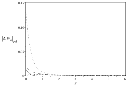
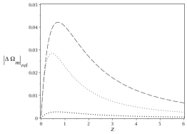
The relative errors of , and are depicted in figure 1 for our and based approximations, as well as the approximations by Scherrer and Sen [50] and Chiba [51], given by the equations (69) and (75), respectively, in appendix A. As can be seen, the previous approximations and the approximant based approximations have similar relative errors for the physical observables and , with respective and maxima, while the approximant yields a maximum relative error of for and an even smaller error for , making this approximation observationally indistinguishable from numerical results. Note that changing so that decreases also decreases the errors, which is due to slower rolling of the scalar field. Note also that the errors of all approximations decrease as increases, which should not come as a surprise since decreasing entails increased matter domination. Investigation of several other scalar field potentials yield similar results.
Tracking quintessence
As our example for tracking quintessence we choose the inverse power law potential, for which
| (63) |
Thus the derivatives of are zero and hence and in (56), while, as for all the present tracking quintessence models, . Thus, , and only involve a single independent parameter, , or, equivalently, , which yields a slightly simpler expressions for and than . Using the system (51) and the value , which form a surface in the state space that intersects the tracker orbit at a point found numerically, and where the numerical calculations also give us , , while is found numerically by integrating151515The present model, like all scalar field models, also admits a 1-parameter set of thawing quintessence solutions in the state space, see [31], which we for brevity do not discuss.
| (64) |
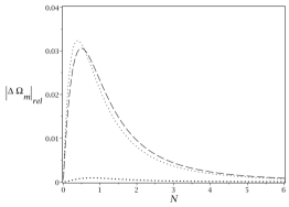
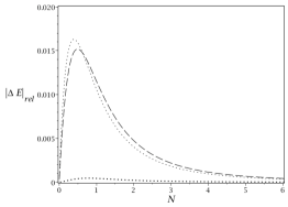
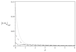
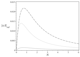
For our relative errors, given in Figure 2, we choose the historically important case , which corresponds to , even though this value is probably too large to provide an observationally viable model. Notably the Chiba approximation [52] for and are rather poor, even more so than the based approximation, which also have relative errors of several , while the based approximations again are excellent with a relative error of for . Decreasing to obtain observationally viable models yields even better results since the maximal errors for the approximations are roughly proportional to , e.g. yields a maximal relative error for . Thus, again the based approximations are observationally indistinguishable from numerical results.
5 Discussion
In this paper we have introduced simple and accurate approximations for thawing and tracking quintessence situated in a broader DE context. This was accomplished by identifying that thawing and tracking quintessence are associated with ‘attractor solutions’ for which (and hence ) and , where for thawing quintessence while for tracking quintessence. These asymptotic properties served as motivation for situating the results in a more general DE setting, which resulted in series expansions in . To improve the accuracy we used Padé approximants where the Padé approximant for was used to relate the approximations to the present time initial value , or, equivalently, .
We note that the Padé approximant contains as many model parameters ( and ) as CPL (, or equivalently , and ) while the approximant has an additional model parameter . However, some potentials yield parameter relationships (or one can impose relationships in the DE context) between , and ; notably the inverse power law potential, , yields , , and thus our approximations for these models contain one less model parameter than CPL; note, however, that to obtain a specific spacetime, one, in addition to model parameters, needs to specify the initial data and , or some equivalent initial data, e.g. and .
In this paper we have followed the majority of work in this area by focussing on generating results from , but there are many other possibilities, as well as further developments and applications, where we describe some in the following list:
-
•
Instead of using as the starting point, one can use other variables. For example, as pointed out in footnote 7, our series expansions also give rise to a series expansion in for and thereby also for . This expansion can subsequently be used to obtain various Padé approximants, which can then serve as the starting point for calculating various other quantities. Or one can derive series expansions for one of the distance measures and use this for constructing Padé approximants, from which other variables and observables can be derived.
-
•
We have here neglected radiation, which, however, can be included in several different ways; one can e.g. use the fixed points on the radiation boundary instead of the present matter boundary when it comes to quintessence, as was done in [38]. Or one can simply add radiation, , to , i.e. , and keep the present expressions, since radiation has a negligible influence on quintessence evolution, and, e.g., use that .
-
•
For some purposes there might be of interest to obtain an expression for how the scalar field changes during thawing quintessence from the past freezing value to some arbitrary -fold time . This can be done in several ways, but constructing the Padé approximant on the righ hand side of in (42b), i.e. where , and then integrating from to yields an excellent approximation161616It is, e.g., a better approximation than that of Raveri et al. [53] given in equation (71) in appendix A. given by
(65) -
•
One can use other dynamical systems variables than the present ones to obtain somewhat different results. For example, we could have used the variables in [31] to deal with tracking quintessence, which would have been useful for the hyperbolic potentials that in addition to the inverse power law potential was dealt with in that paper.171717This would had come with the price that would not have appeared explicitly in the results for and due to the different asymptotic regularization of . However, to improve convergence one should then replace the scalar field variable in [31] with .
-
•
In the spirit of CPL, it is possible to improve our quintessence approximations even further by viewing and as free parameters, not determined by the scalar field potential. This, however, means that one only would do curve fitting, which implies less theoretical content and predictive power.
-
•
We have here focussed on obtaining thawing and tracking quintessence approximations situated in a broader DE context for spatially homogeneous, isotropic and flat spacetimes. A natural next step is to use these approximations in order to interpret the rapidly growing set of increasingly precise observational data. In particular, the present results, or variations thereof, can serve as input in cosmological perturbation theory to bring the results closer to a wide set of observations.
-
•
We finally note that the present approach and variations thereof can easily be applied to other models and theories, especially for those admitting an Einstein frame, although this usually adds parameters thereby further diminishing predictive power.
Acknowledgments
A. A. is supported by FCT/Portugal through CAMGSD, IST-ID, projects UIDB/04459/2020 and UIDP/04459/2020, and by the H2020-MSCA-2022-SE project EinsteinWaves, GA No. 101131233. A.A. would also like to thank the CMA-UBI in Covilhã for kind hospitality. C. U. would like to thank the CAMGSD, Instituto Superior Técnico in Lisbon for kind hospitality.
Appendix A Quintessence approximations and comparisons
In this appendix we review the most prominent quintessence approximations in the literature, including some simplified derivations and extensions; moreover, we will present them in a more unified and concise manner than their original form. We begin with thawing quintessence.
A.1 Thawing quintessence
Let us first derive an approximation introduced by Sherrer and Sen (2008) in [50] and further explored by e.g. Agrawal et al. [54] and Raveri et al. [53]. Instead of using the state vector we construct a dynamical system closely connected with based on the state vector where181818The variable was introduced in [30] while the variable in that paper is just .
| (66) |
which due to (38) yields the dynamical system
| (67a) | ||||
| (67b) | ||||
| (67c) | ||||
Next is assumed to take a frozen constant value while the two last equations in (67) are linearized in only, which results in the following equations for and :
| (68a) | ||||
| (68b) | ||||
where . The second equation, which corresponds to and hence , where yields and thereby the CDM expression for . Inserting this solution into (68a) and integrating gives , from which follows; deparameterizing the solution results in and thereby ; alternatively, solve directly :
| (69a) | ||||
| (69b) | ||||
where the last expression coincides with that of CDM when identifying with (this approximation thereby does not give thawing corrections to the line element since it is just the CDM line element); the above expressions summarize eqs. (23), (25) and (26) in Scherrer and Sen [50]. Taken together with eq. (67a) and this results in
| (70) |
where inserting (69b) yields . This expression agrees with eq. (15) in Agrawal et al. [54] for the exponential potential where is a constant. Integration, with the condition that when and (using and ), results in
| (71) |
where is obtained by inserting (69b). This approximation coincides with eq. (8) in Raveri et al. [53].
Other types of thawing quintessence approximations in the literature are based on series expansions of at some , and thus also of when the latter is regular. An example of this were given by Cahn et al. (2008) [55] who gave approximate expressions for (replacing with in their eq. (15)) and , although note that is missing in their eq. (16), thus hiding that you typically are interested in a domain of . These expressions correspond to the present second order expressions in eqs. (42a) and (42b), whose accuracy we subsequently improved by taking Padé approximants.
Based on earlier results by Dutta and Scherrer (2008) [56], Chiba (2009) [51] Taylor expanded the potential to second order in . By a sequence of ad hoc approximations in the proper time the author derived a series of results (see p. 083517-4 in [51]), which can be extended to also include and , more simply expressed in as follows:
| (72a) | ||||
| (72b) | ||||
| (72c) | ||||
| (72d) | ||||
where
| (73) |
while is given by its CDM expression
| (74) |
The right hand side for was obtained by using and the CDM relation . Taking the limit of equations (72a) and (72b), which corresponds to neglecting the second order Taylor expansion term of the potential, i.e. setting , leads to an indeterminacy that can be solved by L’Hôpital’s rule. In [51] the author also showed how to convert the expression for to the case when , which resulted in the approximation
| (75) |
where
| (76) |
In addition, Chiba [51] discussed the approximation given by Crittenden et al. (2007) [57]. Examining the approximations for a variety of potentials we do not find that gives better approximations than the simpler expressions, which presumably is due to error cancellations and accumulations in a rather uncontrolled manner during the series of ad hoc approximations that resulted in the expressions.
A.2 Tracking quintessence
Here we consider the tracking quintessence approximations given by Chiba (2010) [52], which in turn relied on earlier work by Watson and Scherrer (2003) [58], for the case, and, in particular, , which yields the inverse power law potential. This work is based on a linearized equation for a perturbation of with respect to its asymptotic value . To obtain an improved approximation for the linearized solution for Chiba [52] considered a series expansion in , when expressed in -fold time and the present notation. This is the same series expansion quantity as in the present paper, but in contrast to Chiba [52] we used it to produce approximations for the full non-linear equations; thus, the expansions in the present work coincide with those in [58] and [52] for the quantities that have been computed in those two references up to first order but not for higher orders since Chiba [52] only deals with the linearized equation for . Moreover, there is translation freedom in . In the present work this freedom was fixed by the Padé approximant for , which resulted in an expansion in ; Chiba [52] on the other hand fixed this freedom by, in effect, setting , to obtain the following approximation for :
| (77) |
which in turn yields an approximation for , while the series expansion in for the linearized equation for resulted in
Note that the quantity is related to according to
which corresponds to a translation in with the constant .
As a next step Chiba [52] replaced with , and expanded the resulting expression for in , which yields the following series, here truncated at second order, in :
| (78) |
Note that this is an expansion that is designed to improve the solution for the linear equation for , not the actual solution of the non-linear equation for . The improved linear approximation only improves the actual solution to the extent the linear approximation describes that solution, which, fortunately, to some extent is the case for the inverse power law potential, see e.g., Figure 1 in [28]. Not surprisingly, these approximations yield poorer accuracy than the present ones that are based on approximating the full non-linear equations.
Appendix B Scaling freezing quintessence
In [30] it was demonstrated that in appropriate variables, resulting in a global 3D state space setting, scaling freezing quintessence is associated with a single attractor orbit that constitutes the unstable manifold of an isolated fixed point. The situation and key attractor mechanism is thereby the same as for tracking quintessence. An open set of nearby orbits to the (hyperbolic) saddle fixed point is pushed toward the attractor orbit by a 2D invariant unstable manifold boundary set, for details, see [30] and [31]. The difference with tracking quintessence is that scaling freezing quintessence arises from potentials that have an asymptotic exponential behaviour (that is sufficiently steep).
We therefore consider the situation where , , but where compatibility with nuclear synthesis data requires , see [30] and references therein. Let us further assume that the scalar field, during the time epoch for the attractor solution, rolls down a scalar field potential with where is monotonically decreasing, i.e., we assume that
| (79) |
For our analysis we will consider the dynamical system for the state space vector , which can be obtained from (38):
| (80a) | ||||
| (80b) | ||||
| (80c) | ||||
where now is considered to be a function of , i.e., .
Before continuing, let us note that the simple example of a potential consisting of two exponential terms,
| (81) |
yields
| (82) |
In the present variables, scaling freezing quintessence is associated with the unstable manifold orbit that originates from the fixed point
| (83) |
Next we assume that can be Taylor expanded around , i.e.,
| (84) |
Note that (82) is regular at for the potential with two exponential terms and that
| (85) |
in this case
We can now proceed in the same manner as for thawing and tracking quintessence and first make an expansion based on the unstable eigenvalue, , which leads to expansions in
| (86) |
The fact that and that the eigenvalue involves two parameters, and , result in quite messy expressions for the series expansions. For brevity we will therefore truncate the series already at the linear order in :
| (87a) | ||||
| (87b) | ||||
| (87c) | ||||
where
| (88) |
Using that yields
| (89) |
where
| (90) |
Note that , which leads to that asymptotically toward the past , while decreases toward the future, hence the name scaling freezing.
We leave the higher order series expansions, the construction of Padé approximants, the identification of with present day data, and subsequent investigations, such as error estimates for various potentials, for the interested reader.
References
- [1] Supernova Search Team Collaboration: A. G. Riess et al. Observational evidence from supernovae for an accelerating universe and a cosmological constant. Astron. J., 116:1009, 1998.
- [2] Supernova Cosmology Project Collaboration: S. Perlmutter et al. Measurements of omega and lambda from 42 high redshift supernovae. Astron. J., 517:565, 1999.
- [3] DES Collaboration: T. M. C. Abbott et al. The dark energy survey: Cosmology results with 1500 new high-redshift type ia supernovae using the full 5-year dataset. 2024.
- [4] Planck Collaboration: N. Aghanim et al. Planck 2018 results. vi. cosmological parameters. Astron. Astrophys., 641 A6, 2020.
- [5] W. L. Freedman et al. The carnegie-chicago hubble program viii. an independent determination of the hubble constant based on the tip of the red giant branch. The Astrophysical Journal, 882(1):34, aug 2019.
- [6] A. G. Riess et al. Cosmic distances calibrated to 1% precision with gaia edr3 parallaxes and hubble space telescope photometry of 75 milky way cepheids confirm tension with cdm. The Astrophysical Journal Letters, 908(1):L6, feb 2021.
- [7] A. G. Riess et al. A comprehensive measurement of the local value of the hubble constant with 1 km s-1 mpc-1 uncertainty from the hubble space telescope and the sh0es team. The Astrophysical Journal Letters, 934(1):L7, jul 2022.
- [8] N. Menci et al. Constraints on dynamical dark energy models from the abundance of massive galaxies at high redshifts. The Astrophysical Journal, 900(2):108, sep 2020.
- [9] A. Almeida et al. The eighteenth data release of the sloan digital sky surveys: Targeting and first spectra from sdss-v. The Astrophysical Journal Supplement Series, 267(2):44, aug 2023.
- [10] S. Alam et al. The clustering of galaxies in the completed sdss-iii baryon oscillation spectroscopic survey: cosmological analysis of the dr12 galaxy sample. Monthly Notices of the Royal Astronomical Society, 470(3):2617–2652, 03 2017.
- [11] J. Hou et al. The completed sdss-iv extended baryon oscillation spectroscopic survey: Bao and rsd measurements from anisotropic clustering analysis of the quasar sample in configuration space between redshift 0.8 and 2.2. Monthly Notices of the Royal Astronomical Society, 500(1):1201–1221, 10 2020.
- [12] S. Alam et al. Completed sdss-iv extended baryon oscillation spectroscopic survey: Cosmological implications from two decades of spectroscopic surveys at the apache point observatory. Phys. Rev. D, 103(8):083533, 2021.
- [13] DESI Collaboration: A. G. Adame et al. Desi 2024 vi: Cosmological constraints from the measurements of baryon acoustic oscillations. 2024.
- [14] V. C. Rubin et al. Rotation of the andromeda nebula from a spectroscopic survey of emission regions. Astrophys. J., 159:379, feb 1970.
- [15] V. Trimble. Existence and nature of dark matter in the universe. Annual Rev. Astron. Astrophys., 25:425–472, jan 1987.
- [16] M. Tegmark et al. Cosmological parameters from sdss and wmap. Phys. Rev. D, 69:103501, May 2004.
- [17] R. E. Keeley et al. Jwst lensed quasar dark matter survey ii: Strongest gravitational lensing limit on the dark matter free streaming length to date, 2024.
- [18] D. H. Weinberg et al. Cold dark matter: Controversies on small scales. Proceedings of the National Academy of Sciences, 112(40):12249–12255, feb 2015.
- [19] J. S. Bullock and M. Boylan-Kolchin. Small-scale challenges to the cdm paradigm. Annual Review of Astronomy and Astrophysics, 55:343–387, 2017.
- [20] P. J. E. Peebles and Bharat Ratra. The cosmological constant and dark energy. Rev. Mod. Phys., 75:559–606, 2003.
- [21] DES Collaboration: T. M. C. Abbott et al. Dark energy survey year 1 results: Cosmological constraints from cluster abundances and weak lensing. Phys. Rev. D, 102:023509, Jul 2020.
- [22] A. G. Riess et al. Large magellanic cloud cepheid standards provide a 1% foundation for the determination of the hubble constant and stronger evidence for physics beyond cdm. The Astrophysical Journal, 876(1):85, may 2019.
- [23] E. Di Valentino et al. In the realm of the hubble tension: a review of solutions. Classical and Quantum Gravity, 38(15):153001, jul 2021.
- [24] Le Conte et al. A jwst investigation into the bar fraction at redshifts 1 z 3. Monthly Notices of the Royal Astronomical Society, 530(2):1984–2000, 04 2024.
- [25] M. Chevallier and D. Polarski. Accelerating universes with scaling dark matter. Int. J. Mod. Phys., D10:213, 2001.
- [26] E.V. Linder. Exploring the expansion history of the universe. Phys. Rev. Lett., 90:091301, 2003.
- [27] V. Sahni and A. Starobinsky. Reconstructing dark energy. International Journal of Modern Physics D, 15(12):2105–2132, jan 2006.
- [28] S. Tsujikawa. Quintessence: a review. Class. Quantum Grav., 30:214003, 2013.
- [29] O. Avsajanishvili et al. Observational constraints on dynamical dark energy models. Universe, 10(3:122), 2024.
- [30] A. Alho, C. Uggla, and J. Wainwright. Quintessence from a state space perspective. Physics of the Dark Universe, 39:101146, 2023.
- [31] A. Alho, C. Uggla, and J. Wainwright. Tracking quintessence. Physics of the Dark Universe, 44:101433, 2024.
- [32] R. R. Caldwell and E. V. Linder. Limits of quintessence. Phys. Rev. Lett., 95:141301, 2005.
- [33] A. A. Coley, J. Ibánez, and R. J. van den Hoogen. Homogeneous scalar field cosmologies with an exponential potential. Journal of Mathematical Physics, 38:17, 1997.
- [34] E. J. Copeland, A. R. Liddle, and D. Wands. Exponential potentials and cosmological scaling solutions. Phys. Rev. D, 57:4686, 1998.
- [35] L. A. Urena-Lopez. Unified description of the dynamics of quintessential scalar fields. JCAP, 2012:035, 2012.
- [36] A. Alho and C. Uggla. Scalar field deformations of lambda-cdm cosmology. Phys. Rev. D, 92(10):103502, 2015.
- [37] J. Wainwright and G. F. R. Ellis. Dynamical systems in cosmology. Cambridge University Press, 1997.
- [38] A. Alho and C. Uggla. Quintessential -attractor inflation: A dynamical systems analysis. Journal of Cosmology and Astroparticle Physics, 11:083, 2023.
- [39] P. J. E. Peebles and B. Ratra. Cosmology with a time variable cosmological constant. Astro. Phys. J., 325:L17, 1988.
- [40] B. Ratra and P. J. E. Peebles. Cosmological consequences of a rolling homogeneous scalar field. Phys. Rev. D, 37:3406, 1988.
- [41] B. Ratra and A. Quillen. Gravitational lensing effects in a time-variable cosmological ‘constant’ cosmology. Monthly Notices of the Royal Astronomical Society, 259(4):738–742, 12 1992.
- [42] I. Zlatev, L. Wang, and P. J. Steinhardt. Quintessence, cosmic coincidence and the cosmological constant. Phys. Rev. Lett., 82:896, 1999.
- [43] P. J. Steinhardt, L. Wang, and I. Zlatev. Cosmological tracking solutions. Phys. Rev. D, 59:123504, 1999.
- [44] S. Podariu and B. Ratra. Supernova ia constraints on a time-variable cosmological constant. The Astrophysical Journal, 532(1):109, mar 2000.
- [45] V. Sahni and A.Starobinsky. The case for a positive cosmological lambda-term. Int. J. Mod. Phys. D, 9:373, 2000.
- [46] L.A. Urena-Lopez and T. Matos. New cosmological tracker solution for quintessence. Phys. Rev. D, 62:081302, 2000.
- [47] K. Dimopoulos and C. Owen. Quintessential inflation with -attractors. J. of Cosmology and Astroparticle Physics, 06:027, 2017.
- [48] Y. Akrami et al. Dark energy, -attractors, and large-scale structure surveys. JCAP, 06:041, 2018.
- [49] Y. Akrami et al. Quintessential -attractor inflation: forecasts for stage iv galaxy surveys. JCAP, 04:006, 2021.
- [50] R. J. Scherrer and A. A. Sen. Thawing quintessence with a nearly flat potential. Phys. Rev. D, 77:083515, Apr 2008.
- [51] T. Chiba. Slow-roll thawing quintessence. Phys. Rev. D, 79:083517, 2009.
- [52] T. Chiba. Equation of state of tracker fields. Phys. Rev. D, 81:023515, 2010.
- [53] M. Raveri, W. Hu, and S. Sethi. Swampland conjectures and late-time cosmology. Phys. Rev. D, 99:083518, Apr 2019.
- [54] P. Agrawala, G. Obieda, P. J. Steinhardt, and C. Vafaa. On the cosmological implications of the string swampland. Physics Letters B, 784:271, 2018.
- [55] R. N. Cahn, R. de Putter, and E. V. Linder. Field flows of dark energy. Journal of Cosmology and Astroparticle Physics, 2008(11):015, nov 2008.
- [56] S. Dutta and R. J. Scherrer. Hilltop quintessence. Phys. Rev. D, 78:123525, Dec 2008.
- [57] R. Crittenden, E. Majerotto, and F. Piazza. Measuring deviations from a cosmological constant: A field-space parametrization. Phys. Rev. Lett., 98:251301, Jun 2007.
- [58] C. R. Watson and R. J. Scherrer. Evolution of inverse power law quintessence at low redshift. Phys. Rev. D, 68:123524, 2003.