Adaptive State Observers of Linear Time-varying Descriptor Systems:
A Parameter Estimation-Based Approach

Abstract

In this paper, we apply the recently developed generalized parameter estimation-based observer design technique for state-affine systems to the practically important case of linear time-varying descriptor systems with uncertain parameters. We give simulation results of benchmark examples that illustrate the performance of the proposed adaptive observer.

Parameter estimation, State estimation, Time-varying systems

1 Introduction

One of the most elegant and simple ways to model a physical system is the creation of separate models for standardized subcomponents that can then be pasted together via a network—this procedure leads naturally to models consisting of differential and algebraic equations. These systems are called descriptor systems, singular systems, or differential-algebraic (DAE) systems. The modeling concept mentioned above is used in many modern CAD/modeling systems like SIMULINK, Scicos, MODELICA, and DYMOLA which are applicable to multi-physics problems from different physical domains including mechanical, mechatronic, fluidic, thermic, hydraulic, pneumatic, elastic, plastic or electric components, see [1, 2] for further details. In most modeling systems reduction to an explicit model, if at all possible, is performed with the accompanying loss of accuracy and sparsity—therefore, it is convenient to preserve the DAE structure. Designing control laws for these systems typically requires the knowledge of their state variables. This information is also required in other applications like fault detection and isolation [3]. A lot of research has been reported in the last few years on the development of state observers for this kind of systems, see e.g., [4, 5, 6, 7, 8]. In this paper we are particularly interested in the case of linear time-varying (LTV) descriptor systems—see [9] for an early reference on this topic and [4, 10] for more recent references.

Although there has been a considerable amount of research done on the design of observers for linear time-invariant (LTI) descriptor systems, there has been very little work on the design of observers for LTV ones. This, in spite of the fact that LTV descriptor systems naturally arise from the linearization along a trajectory of nonlinear systems—with the additional difficulty that the linear approximation contains uncertain terms due to the fact that the chosen trajectory is not necessarily a solution of the original system, leading to the presence of uncertain parameters in the DAE model of the system, see [11] for details. In view of the latter reason we are interested here in the design of adaptive observers.

Much of the existing literature on this topic makes extensive use of nonlinear coordinate changes and differentiations of computed quantities, in particular the input signal—a process called completion [4]. While this is theoretically attractive, differentiating signals is not practical due to the presence of noise. It is sometimes argued, that there are some cases, for instance in index three DAE from constrained mechanics, that the derivative of the input signal does not appear in the observer [12]. But it is, of course, of interest to develop a procedure to design observers that does not rely on these non-robust operations. Similarly, we are interested here in the design of (what is called) normal observers [5, Chapter 4], which are described by ordinary differential equations. This, in contrast with singular observers, that are themselves described by DAE, that may exhibit undesirable impulsive behavior [5, 13].

The approach adopted in the paper for the design of our adaptive observers relies on the use of generalized parameter estimation-based observers (GPEBO) recently reported in [14]. The main feature of GPEBO is that the problem of state observation is recasted as a problem of parameter estimation, namely of the systems initial condition. This approach has been proven very successful for the state observation of state-affine systems, which are recast as LTV systems, and many extensions and practical applications to the method have been reported [15, 16, 17, 18, 19]. In a recent paper [20] it was shown that state observation of LTV systems is possible imposing only the (necessary) assumption of observability—a result that should be contrasted with the usual (far stronger) uniform complete observability assumption required by the standard Kalman-Bucy filter solution [21, 22]. Our main objective in this paper is to prove that adopting the GPEBO approach it is possible to generate new, stronger, solutions to the problem of design of adaptive observers for LTV descriptor systems.

Following [13, Section 3], the differences between the LTI and the LTV cases will be underscored in the paper. In particular, we show that assumptions that are always invoked in the LTI case do no play any role in the LTV case. For instance, we show that regularity—a key assumption for LTI systems implied by Conditions A1-A3 of [4, Subsection 2.2.2]—is irrelevant in the LTV case since, as shown in [13, Subsection 3.1], for LTV implicit systems (pointwise) regularity and solvability of the equations are unrelated properties. Another important property of LTV systems is the so-called strangeness index [13, Definition 3.15], which in LTI systems is called the nilpotency index, that plays a central role in the observer design. Indeed, we show that if this index is one then designing a GPEBO is a trivial task. We prove that developing a general theory for observer design in the case of LTV descriptor systems with index larger than one is far from trivial, and some particular solutions are given in that case.

The rest of the paper has the following structure. As an introduction to the general GPEBO theory, in Section 2 we design an adaptive observer for a benchmark example applying GPEBO. In Section 3 we invoke the Standard Canonical Form [24] to develop a general framework for observer design, and solve some specific cases. Section LABEL:sec4 is devoted to the solution using GPEBO of a benchmark circuit example reported in [12, 4], which is described by a descriptor, LTV system. Finally, Section 5 presents some concluding remarks. A preliminary basic lemma used in the GPEBO design is given in Appendix 7.

Notation. $I_{n}$ is the $n\times n$ identity matrix and ${0}_{s\times r}$ is an $s\times r$ matrix of zeros. $\mathbb{R}_{+}$ and $\mathbb{Z}_{+}$ denote the positive real and integer numbers, respectively. For $q\in\mathbb{Z}_{+}$ we define the set $\bar{q}:=\{1,2,\dots,q\}$. For a vector $a\in\mathbb{R}^{n}$, we denote its Euclidean norm by $|a|$ and for a matrix $A\in\mathbb{R}^{n\times m}$ its Euclidean matrix norm is denoted $\|A\|$. The action of a linear time-invariant (LTI) filter ${\cal F}(p)\in\mathbb{R}(p)$ on a signal $w(t)$ is denoted as ${\cal F}(p)[w]$, where $p^{n}[w]:={d^{n}w(t)\over dt^{n}}$. For all time-varying matrices $M:\mathbb{R}_{+}\to\mathbb{R}^{m\times n}$ all properties (e.g., rank) are defined pointwise in time. To avoid dealing with delicate theoretical technical issues related to signals smoothness, we assume that all functions are sufficiently smooth (or analytic) and all differential equations analytically solvable—that is, solutions exist and they are determined by the state initial conditions.

2 An Introduction to GPEBO

In this section we illustrate the GPEBO design with a classical example of an LTV descriptor system with uncertain parameters.

2.1 A motivating example

In this section we consider the following LTV descriptor system with constant uncertain parameters

(1a)

where we defined the matrices

D3 [About the IE assumption] In the LTI case, the IE Assumption 2 is intimately related with observability of the system. As explained in D1 above, in the absence of uncertain parameters we require IE of the simplified regressor $\psi_{0}$ given in (LABEL:psi0). If, moreover $C_{b}=0_{r\times n_{b}}$ then the regressor reduces to $-C_{a}\Phi$ and $A_{0}$ becomes

$$A_{0}=A_{11}-A_{12}A_{22}^{-1}\begin{bmatrix}A_{21}\\ C_{a}\end{bmatrix}.$$

In this case, it can be shown [20] that this regressor is IE if and only if the pair $(A_{0},C_{a})$ is observable.

Hence, even in the LTI case, the relationship between IE and observability of the original system is far from obvious. Clearly, the addition of $C_{b}$ and the time-varying terms increases the possibilities to verify the IE assumption.

D4 [About the parameter estimator] Given the LRE (LABEL:lre) it is possible to implement a classical recursive parameter estimator, e.g., gradient or least-squares [27, 28]. However, it is well-known that to ensure parameter convergence, these schemes impose the highly restrictive assumption of persistent excitation. Namely, that it exists a time window $T>0$ and a constant $\rho>0$ such that

$$\int_{t}^{t+T}\psi(s)\psi^{\top}(s)ds\geq\rho I_{2},\;\forall t\geq 0.$$

It is clear that the IE assumption is significantly weaker than persistent excitation. Actually, it has been shown in [20] that IE is a necessary and sufficient condition for the (on- or off-line) solution of the parameter estimation problem of the LRE $Y=\psi\eta$. See [32] for further discussion on this issue and [33] for a recent survey on new parameter estimators.

D5 [Possible extensions] The assumption on $E$ can be relaxed, we only need to be able to express $x_{b}$ as a function of $x_{a},u$ and $\theta$, as done in (LABEL:xb). Also, notice that the result can be easily extended to systems with delays [15] and external disturbances with uncertain internal model [16, 18].

3 The Standard Canonical Form

One of the main contributions of the paper is the design of a GPEBO for regular, LTV descriptor systems, which are transformed to the standard canonical form [24]. In this section we present this form and introduce an alternative representation for part of the dynamics that is instrumental for the design of the GPEBO, which is carried-out in the next section. For the sake of simplicity, we consider the case of systems without uncertain parameters, in the understanding that—as explained in point D1 of the previous section—this additional feature can be easily accommodated in the observer design.

3.1 Classical representation of the Standard Canonical Form

The lemma below gives a classical representation of the descriptor system, known as the Standard Canonical form [24].

Lemma 3.2.

[34, Subsection 2.6] Consider the analytically solvable LTV descriptor system

[Reason (i)] To explain the first reason define the vector

$$\begin{bmatrix}C^{b}_{\ell,1}(t)\\ C^{b}_{\ell,2}(t)\end{bmatrix}=:C_{w}(t)=\begin{bmatrix}C_{w,1}(t)\\ C_{w,2}(t)\end{bmatrix}$$

and the signal

$$y_{w}:=C_{w}^{\top}(t)z_{w}.$$ (1hjn)

Notice that, due to the condition $C^{b}_{\ell,3}(t)=0$ we have that

$$y_{w}=y_{\ell}-\sum_{i=1}^{n_{a}}C^{a}_{\ell,i}z_{a,i},$$

with the unmeasurable term $z^{b}_{\ell,3}$ absent. We assume in the sequel that the state $z_{a}$ is estimated (exponentially fast) via GPEBO as described in Subsection LABEL:subsec42. Thus, replacing in a certainty-equivalent way, $z_{a}$ by its (easily obtained) estimated value and neglecting the exponentially decaying error term $\hat{z}_{a}(t)-z_{a}(t)$, we can assume that $y_{w}$ is measurable. This is the output that will be associated to the system (LABEL:dotzw).

[Reason (ii)] Regarding the “relative degree” issue (ii) notice that $C_{w}^{\top}(t)B_{w}=C^{b}_{\ell,2}\neq 0$. Consequently, the “relative degree” of the triplet $(C_{w}(t),A_{w}(t),B_{w}(t))$ is one. In the presentation below we restrict ourselves to this case. Although, it is possible to treat also the case of “relative degree” larger than one, the computations are extremely involved, leading to observer designs of little practical interest.

[Reason (iii)] Finally, the stability-related issue (iii) is explained in the proof of the proposition below.

The following assumption is required in the proof of the proposition below.

Assumption 7

There exists a vector $L_{w}(t)\in\mathbb{R}^{2}$ such that the two-dimensional LTV system

$$\dot{\varphi}=\begin{bmatrix}\varphi_{11}&\varphi_{12}\\ \varphi_{21}&\varphi_{22}\end{bmatrix}\varphi,$$

where $\varphi_{11}=L_{w,1}(t)C_{w,1}(t)$, $\varphi_{12}=L_{w,1}(t)C_{w,2}(t)-a_{1}(t)$, $\varphi_{21}=L_{w,2}(t)C_{w,1}(t)+{\dot{C}_{w,1}(t)\over C_{w,1}(t)}$, $\varphi_{22}=L_{w,2}(t)C_{w,2}(t)+{1\over C_{w,2}(t)}[\dot{C}_{w,2}(t)+C_{w,1}(t)a_{1}(t)]$ is exponentially stable.

Proposition 4.8.

Consider the system (LABEL:dotzw), (1hjn) verifying Assumption LABEL:ass5 and with $\dot{C}_{w,2}(t)$ measurable. Define the second order dynamic observer

(1hjoa)

with $L_{w}(t)$ a free vector an

For all systems initial conditions,

$$\lim_{t\to\infty}|\hat{z}_{w}(t)-z_{w}(t)|=0,$$ (1hjop)

exponentially fast, provided $L_{w}(t)$ satisfies Assumption 7.

Proof 4.9.

To establish the proof we derive the dynamics of the observation error $\tilde{z}_{w}:=\hat{z}_{w}-z_{w}$. Hence, we compute

where we used the fact that

$$[G_{w}(t)\ C^{\top}_{w}(t)-I_{2}]B_{w}=0,$$

to get the last identity.

Now, after some lengthy but straightforward calculations, it is possible to prove that

$$M_{w}(t)=\begin{bmatrix}M_{11}&M_{12}\\ M_{21}&M_{22}\end{bmatrix}.$$

where $M_{11}=L_{w,1}(t)C_{w,1}(t)$, $M_{12}=L_{w,1}(t)C_{w,2}(t)-a_{1}(t)$, $M_{21}=L_{w,2}(t)C_{w,1}(t)+{\dot{C}_{w,1}(t)\over C_{w,1}(t)}$, $M_{22}=L_{w,2}(t)C_{w,2}(t)+{1\over C_{w,2}(t)}[\dot{C}_{w,2}(t)+C_{w,1}(t)a_{1}(t)]$.

At this point we make the observation that, if the coefficient $C_{w,1}(t)\equiv 0$, then the matrix $M_{w}(t)$ cannot satisfy Assumption 7. This situation is ruled by Assumption LABEL:ass6. The proof is completed invoking Assumption 7.

Remark 4.10.

A sensible choice for $L_{w}(t)$ is given by

$$L_{w}(t)=\begin{bmatrix}{a_{1}(t)\over C_{w,2}(t)}\\ \\ -{\dot{C}_{w,1}(t)\over C^{2}_{w,1}(t)}\end{bmatrix}$$

which diagonalizes the matrix $M_{w}(t)$. Then, the stability test boils down to integrability of the resulting diagonal terms.

Remark 4.11.

It is possible to prove that in the LTI case Assumption 7 is satisfied with the choice

$$L_{w}=a_{1}C_{w,1}\begin{bmatrix}{C_{w,1}\over C_{w,2}}\\ 1\end{bmatrix},$$

provided $a_{1}{C_{w,1}\over C_{w,2}}<0.$ From (LABEL:dotzw) it is clear that it is possible to “change the sign” of the coefficient $a_{1}$ introducing a change of coordinates $z_{w}^{\prime}=\begin{bmatrix}1&0\\ 0&-1\end{bmatrix}z_{w}$. Hence, Assumption 7 can always be satisfied in the LTI case. Actually, in view of Remark LABEL:rem1 the design of the observer of $z_{b}$ for LTI systems can be significantly simplified.

5 A Benchmark LTV Circuit Example

In [12, Chapter 6]—see also [4, Section 7]—the circuit example depicted in Fig. 1 is considered, with the capacitors, inductor and resistors time-varying. A state observer is designed invoking the systems completion procedure that, as explained in the Introduction, entails the calculation of signal derivatives. Here, we propose a GPEBO-based solution.

Figure 1: Circuit example from [12, Chapter 6].

As shown in [4] the dynamic behavior of the circuit may be written in the form

where $x:=\mbox{col}(e_{1},e_{2},i_{l},i_{r_{1}},i_{r_{2}},i_{v})$, $u:=V$ and

$$E(t) =\begin{bmatrix}{C_{a}(t)}&0&0&0&0&0\\ 0&{C_{b}(t)}&0&0&0&0\\ 0&0&{L(t)}&0&0&0\\ 0&0&0&0&0&0\\ 0&0&0&0&0&0\\ 0&0&0&0&0&0\end{bmatrix},B=\begin{bmatrix}0\\ 0\\ 0\\ 0\\ 0\\ -1\end{bmatrix}$$

$$A(t) =\begin{bmatrix}-\dot{C}_{1}(t)&0&0&1&-1&1\\ 0&-\dot{C}_{2}(t)&-1&-1&0&0\\ 0&1&-\dot{L}(t)&0&0&0\\ -1&1&0&R_{1}(t)&0&0\\ -1&0&0&0&R_{2}(t)&0\\ -1&0&0&0&0&0\end{bmatrix}.$$

Similarly to [4] we consider that the output matrix is of the form

$$C=\begin{bmatrix}0&0&1&0&0&1\end{bmatrix}.$$

Partitioning $x=\mbox{col}(x_{a},x_{b})$, with $x_{a}(t)\in\mathbb{R}^{3},x_{b}(t)\in\mathbb{R}^{3}$, we can rewrite our system in the form

with

$$A_{11} :=\begin{bmatrix}-\frac{\dot{C}_{1}}{C_{1}}&0&0\\ 0&-\frac{\dot{C}_{2}}{C_{2}}&-\frac{1}{C_{2}}\\ 0&\frac{1}{L}&-\frac{\dot{L}}{L}\end{bmatrix},\;A_{12}=\begin{bmatrix}\frac{1}{C_{1}}&-\frac{1}{C_{1}}&\frac{1}{C_{1}}\\ -\frac{1}{C_{2}}&0&0\\ 0&0&0\end{bmatrix},$$

$$A_{21} :=\begin{bmatrix}-1&1&0\\ -1&0&0\\ -1&0&0\end{bmatrix},\;A_{22}:=\begin{bmatrix}R_{1}&0&0\\ 0&R_{2}&0\\ 0&0&0\end{bmatrix},$$

and $C_{a}=C_{b}:=\begin{bmatrix}0&0&1\end{bmatrix}$. Similarly to the example of Subsection 2.1, we assume that the capacitors and inductors are bounded away from zero, and rewrite the system as

with

$${\cal A}_{b}:=\begin{bmatrix}A_{22}\\ C_{b}\end{bmatrix}=\begin{bmatrix}R_{1}&0&0\\ 0&R_{2}&0\\ 0&0&0\\ 0&0&1\end{bmatrix}.$$

This matrix is clearly full rank and injective, hence it satisfies Assumption 1. Consequently, to invoke Proposition LABEL:pro1 for the design of the GPEBO, it only remains to verify the IE Assumption 2 of the regressor $\psi$ defined in (LABEL:regpsi).

For simulations we followed [12, Chapter 6] and considered the functions below for the circuit elements:

$$C_{1}(t) =3+\cos(t/3),\;C_{2}(t)=2-\cos(2t),$$

$$L(t) =2-\exp(-t),$$

$$R_{1}(t) =-(4+2\sin(t)),\;R_{2}(t)=-(2+\sin(t)),$$

and the voltage input signal $u(t)=4\cos(2t)\sin(t/5)$. The initial conditions for the system were taken as $x_{a}(0)=\mbox{col}(0,1,2)$ and ${x_{b}(0)=\mbox{col}(0.25,0,-0.25)}$ and for the estimators dynamic extension as $\xi_{a}(0)=\mbox{col}(1,0,0)$.

Following [32] the estimation was carried out with Kreisselmeier regression extension [32, Section IV.B], the standard mixing step [32, Section II.B] and the classical gradient estimator [32, Equation (10)]. The filters were selected as ${\cal K}(p)={\lambda\over p+\lambda}$ with $\lambda=\mbox{diag}\{0.1,0.2,0.3\}$ and the gradient gain chosen as $\gamma=10^{10}$.

The simulation results for the regressor $\psi$ are shown in Fig. 2, which clearly shows that it is IE. The behavior of the remaining signals of interest is depicted in Figs. 3-8. To illustrate the effect of the adaptation gain $\gamma$ on the transient behavior, in Figs, 6-8 we show the result for two different values of this gain. As expected, increasing the gain accelerates the convergence.

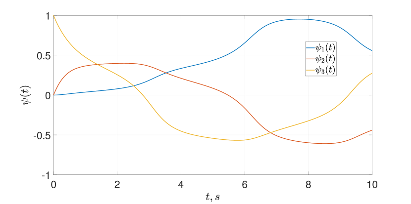
Figure 2: Transients of the regressor $\psi$

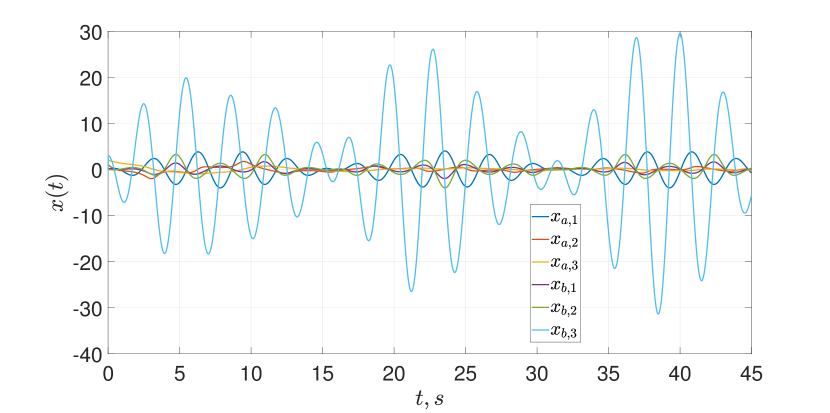
Figure 3: Transients of the state vector

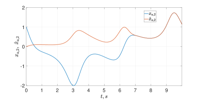
Figure 4: State $x_{a}$ and state estimation $\hat{x}_{a}$

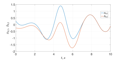
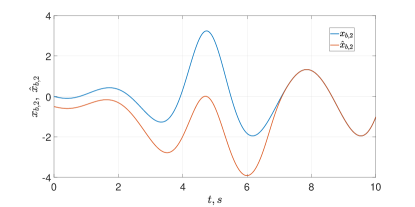
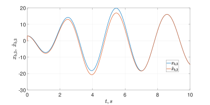
Figure 5: State $x_{b}$ and state estimation $\hat{x}_{b}$

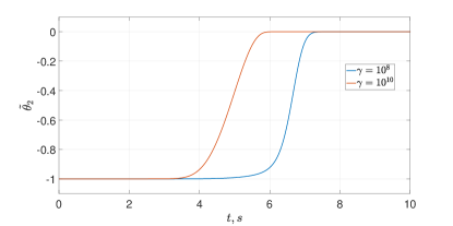
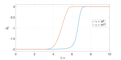
Figure 6: Initial conditions estimation error $\tilde{\theta}~{}:=~{}\hat{\theta}-\theta$, where $\theta~{}:=~{}\xi_{a}(0)-x_{a}(0)$, for two gradient adaptation gains.

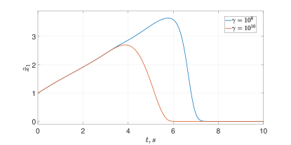
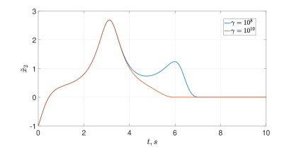
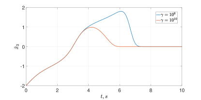
Figure 7: State estimation error $\tilde{x}_{a}:=\hat{x}_{a}-{x}_{a}$, for two gradient adaptation gains.

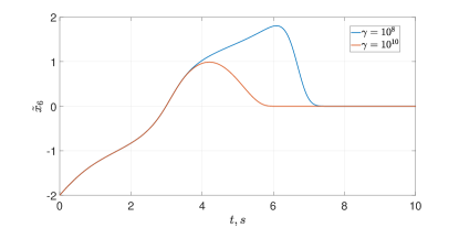
Figure 8: State estimation error $\tilde{x}_{b}:=\hat{x}_{b}-{x}_{b}$, for two gradient adaptation gains.

6 Concluding Remarks and Future Research

We have presented in this paper a first attempt to develop a comprehensive theory for the design of observers for general LTV descriptor systems. A consequence of our intention to keep the analysis as general as possible is that the final results are a little bit cryptic. Certainly, proceeding from this general framework, we can address particular cases and achieve some practically workable designs.

We have identified several critical aspects of the problem. For instance, the highly relevant role played by the strangeness index—see Subsection LABEL:subsec41. Intensive research has been carried out to develop procedures to render the system strangeness-free, see [13, 2] for some results along these lines. Our current work is aimed at applying these techniques for the problem of observer design and we expect to be able to report some results soon. We have also underscored the differences between the LTV and the LTI case, which are quite significant.

Another research line that we are pursuing is to develop the theory for particular classes of LTV descriptor systems, with special emphasis on practical examples. In this respect a class of systems of great relevance are the ones described by port-Hamiltonian models.

7 Background Material

To design the proposed observer we rely on the following well-known fact, whose proof may be found in [37, Section C.4].

Fact 1.

Consider the system

$$\dot{\mathrm{z}}(t)={\mathbb{A}}(t){\mathrm{z}}(t),\quad{\mathrm{z}}(0)=z_{0}\in\mathbb{R}^{n},$$ (1hjoq)

with ${\mathrm{z}}(t)\in\mathbb{R}^{n}$ and ${\mathbb{A}}(t)\in\mathbb{R}^{n\times n}$, and the auxiliary linear $n\times n$ matrix differential equation

$$\dot{\mathbb{Z}}(t)={\mathbb{A}}(t){\mathbb{Z}}(t),\quad{\mathbb{Z}}(0)=I_{n},$$ (1hjor)

with ${\mathbb{Z}}(t)\in\mathbb{R}^{n\times n}$. The solution of (1hjor) satisfies

$${\mathbb{Z}}(t)=\Phi(t)$$

where $\Phi(t)$ is the state transition matrix of the system (1hjoq). Consequently, the trajectories of the system (1hjoq) verify

$${\mathrm{z}}(t)={\mathbb{Z}}(t){\mathrm{z}}_{0}.$$

∎

References

[]Romeo Ortega (Fellow, IEEE) was born in Mexico. He obtained his B.S. in Electrical and Mechanical Engineering from the National University of Mexico, Master of Engineering from Polytechnical Institute of Leningrad, USSR, and the Docteur d‘Etat from the Polytechnical Institute of Grenoble, France in 1974, 1978 and 1984, respectively.

He then joined the National University of Mexico, where he worked until 1989. He was a Visiting Professor at the University of Illinois in 1987–1988 and at the McGill University in 1991–1992, and a Fellow of the Japan Society for Promotion of Science in 1990–1991. He has been a member of the French National Researcher Council (CNRS) since June 1992. Currently, he is in the Laboratoire de Signaux et Systemes (SUPELEC) in Paris. His research interests are in the fields of nonlinear and adaptive control, with special emphasis on applications.

Dr. Ortega has published three books and more than 350 scientific papers in international journals, with an h-index of 97. He has supervised more than 35 Ph.D. theses. He is a Fellow Member of the IEEE since 1999 and an IFAC fellow since 2016. He has served as Chairman in several IFAC and IEEE committees and participated in various editorial boards of international journals. Currently he is Editor in Chief of Int. J. Adaptive Control and Senior Editor of Asian J. of Control.

[]Alexey Bobtsov received the M.S. degree in Electrical Engineering from ITMO University, St. Petersburg, Russia in 1996, received his Ph.D. in 1999 and the degree of Doctor of Science (habilitation thesis) in 2007 from the same University. From December 2000 to May 2007 Dr. Bobtsov served as Associate Professor of Department of Control Systems and Informatics. In May 2007 Dr. Bobtsov was appointed as Professor of Department of Control Systems and Informatics. In September 2008 he was elected as the Dean of Computer Technologies and Controlling Systems Faculty. He is currently a Director of School of Computer Technologies and Control at ITMO University. He is a Senior Member of IEEE since 2010. He is a Member of International Public Association Academy of Navigation and Motion Control. He is a co-author of more than 250 journal and conference papers, 20 books and textbooks. His research interests are in fields of nonlinear and adaptive control.

[]Fernando Castaños received the B.Eng. degree in electric and electronic engineering and the M.Eng. degree in control engineering from the Universidad Nacional Autónoma de México, Mexico City, Mexico, in 2002 and 2004, respectively, and the Ph.D. degree in control theory from Université Paris-Sud XI, Paris, France, in 2009.

He was a Postdoctoral Fellow with the Center for Intelligent Machines, McGill University, Montréal, QC, Canada, for two years. Since 2011, he has been with the Departamento de Control Automático, CINVESTAV-IPN, Mexico City. His research interests include variable structure systems, passivity-based control, nonlinear control, port-Hamiltonian systems, and robust control. Dr. Castaños is an Editor for International Journal of Robust and Nonlinear Control.

[]Nikolay Nikolaev received the M.S. degree in electrical engineering from ITMO University, St. Petersburg, Russia in 2003, received his PhD in 2006 from the same University. From 2002 until 2013 he worked as Engineer of Department of Control Systems Design for Power Plants at JSC Kirovsky Zavod (Kirov Plant). From 2013 he is an Associate Professor in Department of Control Systems and Robotics from ITMO University. He is a Member of IEEE since 2006. His research interests are in fields of nonlinear and adaptive control.

References

- [1] A. Ilchmann and T. Reis, Surveys in Differential-Algebraic Equations I. Springer Berlin, Heidelberg, 2013.
- [2] V. Mehrmann and B. Unger, “Control of port-hamiltonian differential-algebraic systems and applications,” Acta Numerica, vol. 32, pp. 395–515, 2023.
- [3] R. J. Patton, P. M. Frank, and R. N. Clark, Issues of fault diagnosis for dynamic systems. Springer London, 2000.
- [4] K. S. Bobinyec and S. L. Campbell, Linear Differential Algebraic Equations and Observers. Cham: Springer International Publishing, 2015, pp. 1–67.
- [5] L. Dai, Singular Control Systems. Springer Berlin, Heidelberg, 1989.
- [6] M. Darouach, “On the functional observers for linear descriptor systems,” Systems & Control Letters, vol. 61, no. 3, pp. 427–434, 2012.
- [7] M. Hou and P. Muller, “Design of observers for linear systems with unknown inputs,” IEEE Transactions on Automatic Control, vol. 37, no. 6, pp. 871–875, 1992.
- [8] P. Muller and M. Hou, “On the observer design for descriptor systems,” IEEE Transactions on Automatic Control, vol. 38, no. 11, pp. 1666–1671, 1993.
- [9] S. L. Campbell, F. Delebecque, and R. Nikoukhah, “Observer design for linear time-varying systems descriptor systems,” Proc. Control Industrial Systems (CIS97), Belfort, France, pp. 507–512, 1997.
- [10] I. I. Zetina-Rios, M. Alma, G. L. Osorio-Gordillo, M. Darouach, and C. M. Astorga-Zaragoza, “Generalized adaptive observer design for a class of linear algebro-differential systems,” in 2023 IEEE 11th International Conference on Systems and Control (ICSC), 2023, pp. 171–176.
- [11] S. L. Campbell, “Linearization of daes along trajectories,” Zeitschrift für angewandte Mathematik und Physik ZAMP, vol. 46, no. 1, pp. 70–84, 1995.
- [12] K. S. Bobinyec, Observer construction for systems of differential algebraic equations using completions. North Carolina State University, 2013.
- [13] P. Kunkel, Differential-algebraic equations: analysis and numerical solution. European Mathematical Society, 2006, vol. 2.
- [14] R. Ortega, A. Bobtsov, N. Nikolaev, J. Schiffer, and D. Dochain, “Generalized parameter estimation-based observers: Application to power systems and chemical–biological reactors,” Automatica, vol. 129, p. 109635, 2021.
- [15] V. Bezzubov, A. Bobtsov, D. Efimov, R. Ortega, and N. Nikolaev, “Adaptive state observation of linear time-varying systems with delayed measurements and unknown parameters,” International Journal of Robust and Nonlinear Control, vol. 33, no. 2, pp. 1203–1213, 2023.
- [16] B. Y. Alexey Bobtsov, Romeo Ortega and N. Nikolaev, “Adaptive state estimation of state-affine systems with unknown time-varying parameters,” International Journal of Control, vol. 95, no. 9, pp. 2460–2472, 2022.
- [17] A. Bobtsov, N. Nikolaev, R. Ortega, and D. Efimov, “State observation of LTV systems with delayed measurements: A parameter estimation-based approach with fixed convergence time,” Automatica, vol. 131, p. 109674, 2021.
- [18] A. Pyrkin, A. Bobtsov, R. Ortega, and A. Isidori, “An adaptive observer for uncertain linear time-varying systems with unknown additive perturbations,” Automatica, vol. 147, p. 110677, 2023.
- [19] J. G. Romero and R. Ortega, “Adaptive state observation of linear time-varying systems with switching unknown parameters: Application to gain scheduling and event-triggered control,” International Journal of Adaptive Control and Signal Processing, vol. 37, no. 11, pp. 2915–2933, 2023.
- [20] L. Wang, R. Ortega, and A. Bobtsov, “Observability is sufficient for the design of globally exponentially stable state observers for state-affine nonlinear systems,” Automatica, vol. 149, p. 110838, 2023.
- [21] P. Bernard, Observer design for nonlinear systems. Springer, 2019, vol. 479.
- [22] W. J. Rugh, Linear system theory (2nd ed.). Prentice-Hall, Inc., 1996.
- [23] A. ILCHMANN, Contributions to Time-Varying Linear Control Systems. Verlag an der Lottbek, 1989.
- [24] S. L. Campbell and L. R. Petzold, “Canonical forms and solvable singular systems of differential equations,” SIAM Journal on Algebraic Discrete Methods, vol. 4, no. 4, pp. 517–521, 1983.
- [25] A. Bunse-Gerstner, R. Byers, V. Mehrmann, and N. K. Nichols, “Feedback design for regularizing descriptor systems,” Linear algebra and its applications, vol. 299, no. 1-3, pp. 119–151, 1999.
- [26] S. L. Campbell and C. D. Meyer, Generalized inverses of linear transformations. SIAM, 2009.
- [27] S. Sastry and M. Bodson, Adaptive control: stability, convergence and robustness. Prentice-Hall, New Jersey, 1989.
- [28] G. Tao, Adaptive Control Design and Analysis, ser. Adaptive and Cognitive Dynamic Systems: Signal Processing, Learning, Communications and Control. Wiley, 2003.
- [29] R. Ortega, J. G. Romero, and S. Aranovskiy, “A new least squares parameter estimator for nonlinear regression equations with relaxed excitation conditions and forgetting factor,” Systems & Control Letters, vol. 169, p. 105377, 2022.
- [30] G. Kreisselmeier and G. Rietze-Augst, “Richness and excitation on an interval-with application to continuous-time adaptive control,” IEEE Transactions on Automatic Control, vol. 35, no. 2, pp. 165–171, 1990.
- [31] P. Kunkel, V. Mehrmann, and W. Rath, “Analysis and numerical solution of control problems in descriptor form,” Mathematics of Control, Signals and Systems, vol. 14, pp. 29–61, 2001.
- [32] R. Ortega, S. Aranovskiy, A. A. Pyrkin, A. Astolfi, and A. A. Bobtsov, “New results on parameter estimation via dynamic regressor extension and mixing: Continuous and discrete-time cases,” IEEE Transactions on Automatic Control, vol. 66, no. 5, pp. 2265–2272, 2021.
- [33] R. Ortega, V. Nikiforov, and D. Gerasimov, “On modified parameter estimators for identification and adaptive control. a unified framework and some new schemes,” Annual Reviews in Control, vol. 50, pp. 278–293, 2020.
- [34] S. Trenn, Solution Concepts for Linear DAEs: A Survey. Berlin, Heidelberg: Springer Berlin Heidelberg, 2013, pp. 137–172.
- [35] M. Tranninger, H. Niederwieser, R. Seeber, and M. Horn, “Unknown input observer design for linear time-invariant systems—a unifying framework,” International Journal of Robust and Nonlinear Control, vol. 33, no. 15, pp. 8911–8934, 2023.
- [36] J. Dávila, L. Fridman, and A. Levant, “Robust state estimation for linear time-varying systems using high-order sliding-modes observers,” in Sliding-Mode Control and Variable-Structure Systems: The State of the Art. Springer, 2023, pp. 133–162.
- [37] E. D. Sontag, Mathematical control theory: deterministic finite dimensional systems. Springer Science & Business Media, 2013, vol. 6.
[![[Uncaptioned image]](/html/2407.14373/assets/biog/Romeo_Ortega.jpg) ]Romeo Ortega (Fellow, IEEE) was born in Mexico. He obtained his B.S. in Electrical and Mechanical Engineering from the National University of Mexico, Master of Engineering from Polytechnical Institute of Leningrad, USSR, and the Docteur d‘Etat from the Polytechnical Institute of Grenoble, France in 1974, 1978 and 1984, respectively.