Time-dependent condensate formation in ultracold atoms with energy-dependent transport coefficients
Abstract
Time-dependent Bose–Einstein condensate (BEC) formation in ultracold atoms is investigated in a nonlinear diffusion model. For constant transport coefficients, the model has been solved analytically. Here, we extend it to include energy-dependent transport coeffcients and numerically solve the nonlinear equation. Our results are compared with the earlier analytical model for constant transport coeffcients, and with recent deep-quench data for 39K at various scattering lengths. Some non-physical predictions from the constant-coefficient model are resolved using energy-dependent drift and diffusion.
I Introduction
Time-dependent Bose–Einstein condensate formation in ultracold quantum gases is an ideal testing ground for nonequilibrium-statistical models and theories. Following the early 1995 BEC discoveries in alkali atoms, the time-dependence of condensate formation in the course of evaporative cooling was first studied 1998 in 23Na [1] and compared with available numerical model results [2]. Here, a short radio-frequency pulse was used to remove high-energy atoms in order to investigate the subsequent time-dependent thermalization and transition to the condensed state.
Much more precise experimental data with error bars were obtained 2002 for 87Rb [3], where cooling into the quantum-degenerate regime was achieved by continuous evaporation for a duration of several seconds. The data were compared with the results of a numerical model based on quantum kinetic theory [4] that had been developed at a time when no data were available, predicting a thermalization timescale for 87Rb of the order of 5 seconds, more than one order of magnitude larger than the one for 23Na. The model was later adapted to the data [3] when the measured thermalization timescale in rubidium turned out to be similar to the one in sodium.
For a detailed comparison of nonequilibrium-statistical models for time-dependent BEC formation and data, it appears more promising to start from a thermalized atomic cloud in a trap that is subjected to a short deep quench, because the initial condition is fixed and not time-varying as in continuous evaporative cooling. Corresponding time-resolved data were provided by the Cambridge group in 2021 using a homogeneous 3D Bose gas of 39K with tunable interactions and near-perfect isolation in a cylindrical optical box [5]. We have compared these data with results of our nonlinear diffusion model [6, 7] in Ref. [8]. At four different interaction strengths, we found agreement with the data already for constant transport coefficients, where the model is analytically solvable for deep-quench initial conditions given by a truncated Bose–Einstein distribution, and boundary conditions at the singularity [9].
In the present work, we extend this approach to energy-dependent transport coefficients. This case is physically more realistic, and artifacts of the analytical solution can be resolved. On the downside, the nonlinear boson diffusion equation (NBDE) is no longer solvable with analytical methods. However, in the limit of constant coefficients, the precision of our numerical solution can be checked through a comparison with the exact result, which is rarely possible in other kinetic approaches, with the exception of a linear relaxation-time approximation to the nonlinear thermalization problem.
In the following section, we briefly review the nonlinear boson diffusion model, and its analytical solution for constant coefficients. Energy-dependent drift and diffusion coefficients are introduced in Sect. III, the numerical solution of the nonlinear equation is presented, and in the special case of constant transport coefficients compared with the available exact solution. The time-dependent condensate fraction for 39K following a deep quench that removes 77% of the atoms and of the energy is calculated numerically for various scattering lengths in Sect. IV, and compared to the Cambridge data. The conclusions are drawn in Sect. V.
II Nonlinear diffusion model
With our previously developed [6, 7] nonlinear model we have already computed the nonequilibrium evolution and time-dependent condensate formation in equilibrating Bose gases of ultracold atoms using constant transport coefficients for 23Na [10], and more recently [8] with a comparison to deep-quench data [5] for 39K. We describe the cold-atom vapor in a trap as a time-dependent mean field with a collision term and consider only -wave scattering with the corresponding scattering lengths. The -body density operator is composed of single-particle wave functions of the atoms which are solutions of the time-dependent Hartree-Fock equations plus a time-irreversible collision term . The latter causes the system to thermalize through random two-body collisions ()
| (1) |
The self-consistent Hartree-Fock mean field of the atoms is , where the trap provides an external potential.
The full many-body problem can be reduced to the one-body level in an approximate version for the ensemble-averaged single-particle density operator by taking the trace over particles . Its diagonal elements represent the probability for a particle to be in a state with energy
| (2) |
The total number of particles is . We neglect the off-diagonal terms of the density matrix, because their time evolution mainly consists of a loss term that tends to dissipate away the non-diagonal elements generated by the time evolution of the mean field, as was shown for fermions [11], and is expected to occur similarly for bosons.
The many-body Hartree-Fock term is reduced to the one-body level as well, with the mean-field Hamiltonian plus the confining potential that represents the trap, but in the following we concentrate on the collision term that causes the thermalization of the system, and also drives the time-dependent formation of the Bose–Einstein condensate.
Assuming sufficient ergodicity as has been widely discussed in the literature [12, 13, 14, 15, 16, 17], the occupation-number distribution in a finite Bose system obeys a Boltzmann-like collision term, where the distribution function depends only on energy and time. For elastic two-body interactions, the equation for the single-particle occupation numbers can be expressed as [6]
| (3) | |||
with the second moment of the interaction and the function , which ensures energy conservation. In an infinite system, it would be a -function as in the usual Boltzmann collision term where the single-particle energies are time independent,
| (4) |
In a finite system, however, the energy-conserving function acquires a width, such that off-shell scatterings between single-particle states which lie apart in energy space become possible [11].
The reduction to dimensions corresponds to spatial and momentum isotropy. For the thermal cloud of cold atoms surrounding a Bose–Einstein condensate (BEC), this is expected to be approximately fulfilled. Different spatial dimensions enter our present formulation through the density of states, which depends also on the type of confinement. The model calculations in this work are for a 3D system, and as in the 39K experiment [5], we investigate results for the density of states of bosonic atoms confined in a cylindrical optical box.
From the above quantum Boltzmann collision term, we had derived in [6, 7] the nonlinear boson diffusion equation (NBDE) for the single-particle occupation probability distributions as
| (5) |
The drift term accounts for the shift of the distribution towards the infrared, the diffusion function for the broadening with increasing time. Both transport coefficients are defined in terms of moments of the transition probabilities. In the present case of a deep quench in a thermalized vapor, the diffusion coefficient causes the softening of the sharp cut at in the UV that signifies the quench, as well as the diffusion of particles into the condensed state in the IR. The many-body physics is contained in these transport coefficients, which depend on energy, time, and the second moment of the interaction. The derivative term of the diffusion coefficient in the NBDE (5) causes the stationary solution to become a Bose–Einstein distribution, which is attained for as
| (6) |
under the condition that the ratio has no energy dependence, and requiring that . (We use units throughout this manuscript). The chemical potential is in a finite Bose system. It appears as an integration constant in the stationary solution of Eq. (5) for . It vanishes in case of inelastic collisions that do not conserve particle number such that the temperature alone determines the equilibrium distribution.
In the limit of energy-independent transport coefficients , the fluctuation-dissipation relation is simply , and the NBDE can be solved analytically through a nonlinear transformation [6, 7]. It is one one the few nonlinear partial differential equations that have a clear physical meaning and can be solved exactly. The solution is
| (7) |
with the time-dependent partition function that fulfills the linear diffusion (heat) equation
| (8) |
The time-dependent partition function and its energy-derivative are given analytically, but still require integrals over the bounded Green’s function of the linear problem and an exponential function that contains an energy-integral over the initial distribution. However, for certain simplified initial conditions such a theta-function [6], or a truncated Bose–Einstein distribution [9]
| (9) |
exact analytical results have been obtained and used in comparisons of the time-dependent condensate fraction to data [10, 8]. For the present case of a Bose–Einstein distribution at temperature truncated via a deep quench at an energy such that the temperature of the final equilibrium distribution becomes , the generalized partition function can be expressed as an infinite series [9]
| (10) |
and similarly for the energy-derivative of . The exact analytical expressions for are combinations of exponentials and error functions. The distribution function can now be computed directly from Eq. (7). The convergence of the solutions has been studied in Ref. [10]: a result with expansion coefficients – depending on the system and the observable – is indistinguishable from the exact solution with . The infinite series terminates in case is an integer due to the binomial coefficient, and we explicitly use that property for 39K, where the exact solution are obtained for . A brief summary of the nonlinear diffusion model with constant transport coefficients for both, boson and fermion systems at low and high energies and temperatures is presented in Ref. [7].
III NBDE with energy-dependent drift and diffusion
Whereas the exact solution for constant transport coefficients already yields physically reasonable results, it also has drawbacks. For example, when calculating the time-dependent condensate fraction using the additional condition of particle-number conservation, it may slightly overshoot the equilibrium value and approach it from above at later times: A large constant drift towards the IR causes thermalization in the UV region to be too slow, such that at large times the Bose–Einstein limit is reached in the IR, but not yet in the UV, resulting in an unbalanced energy-dependent equilibration. Although this effect is often hardly visible in a plot, it is a deficiency of the constant-coefficient case that can be remedied using energy-dependent drift and diffusion coefficients.
For energy-dependent transport coefficients, we presently cannot solve the NBDE (5) analytically, although for simplified cases such as constant diffusion and linear drift one may try to find solutions. We shall therefore resort to numerical solutions using the Julia programming language. In the limiting case of constant transport coefficients, we shall compare the numerical solutions to the exact results in order to assess the accuracy of the numerical approach.
III.1 Energy dependence of the transport coefficients
We seek energy-dependent transport coefficients that cause a faster thermalization in the region and yield the correct final distribution of particles in the limit . In a semi-classical description, the diffusion at is zero such that particles with zero momentum cannot contribute to the transport of particles into non-zero energy states. However, in a quantum description, the transport coefficients at can take a finite value, denoted as and . For a system of bosons, which has a singularity at the chemical potential, a time-independent boundary condition can be assigned at . The position of the singularity is then fixed, the one-particle distribution function does not change with time at , and the constraint at applies. For an initial distribution without a singularity at the chemical potential, like a box distribution for a gluon system at relativistic energies, a time-dependent boundary at is, however, required.
The solution of the nonlinear boson diffusion equation should still converge to the Bose–Einstein equilibrium distribution for . Therefore, when substituting with in Eq. (5), the following stationary nonlinear diffusion equation must hold
| (11) | ||||
| (12) |
which is an inhomogeneous partial differential equation for depending on a unknown function and has the general solution
| (13) |
The integral over is
| (14) |
such that the integrals inside the square brackets in Eq. (13) simplify to
| (15) | |||
| (16) |
Applying now the constraint and inserting the Bose–Einstein distribution for yields the previously discussed relation between the transport coefficients
| (17) |
Hence, for each time step at any energy, the relation has to be fulfilled to reach the desired Bose–Einstein distribution in the stationary limit.
To obtain a system that thermalizes into a condensed and non-condensed phase, one has to undercut the critical temperature . Experimentally this is done by evaporative cooling or by sudden energy quenches, such that all particles with an energy are removed from the trap. Therefore one can steer the final temperature by changing the quench energy and one gets , where is the initial temperature before the quench and is the equilibrium temperature that is eventually reached after removing higher-energy particles from the trap. In [10] it is shown that no condensate forms if the final temperature at the critical number density stays above the critical temperature for bosonic atoms of mass ,
| (18) |
where we neglect the effects of interactions [18] at the moment.
The order of for a non-relativistic
3D gas inside a box trap is and hence the final temperatures of experimentally reasonable setups range between and for common BEC experiments with 87Rb, 39K, 23Na and 7Li of approximately particles inside a box trap.
In the simplified model with constant transport coefficients, the values of and are connected to the equilibrium temperature and the local thermalization time . This relationship arises from the equality of the stationary solution of the nonlinear diffusion equation with the Bose–Einstein distribution. The thermalization time at the cut has been deduced from an asymptotic expansion of error functions in the analytical solutions of the non-linear diffusion equation for a theta-function initial condition, as [6]. For a general initial distribution with a cut at , it can be expressed as
| (19) |
where for fermions and for bosons in the case of an initial theta-function distribution. The analytical result for a truncated Bose–Einstein initial distribution has not been derived yet but is expected to be considerably shorter than that for a theta-function distribution because the shape of the initial distribution resembles already the final Bose–Einstein result. For 39K, was adopted in [8] to calculate the transport coefficients such that they align with the thermalization time of experimental data. With being a required experimental constant, the transport coefficients for the analytical solution of the nonlinear Boltzmann diffusion equation are thus determined by
| (20) | ||||
| (21) |
( nK, nK) (nK2/ms) (nK/ms) (ms) (ms) 140 0.08 130 600 280 0.16 65 300 400 0.229 46 210 800 0.457 23 105
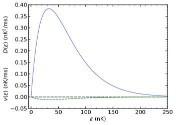
We use this calculation of the constant transport coefficients to later normalize the energy-dependent transport coefficients. To model energy-dependent transport coefficients that obey Eq. (17), have an energy-average matching the value of the constant transport coefficients, and constant or zero limits for large energies, a wide class of smooth functions is available. To accelerate thermalization in the region , the diffusion in this energy region must be increased compared to the constant-coefficient case. Since the thermal tail does not contribute significantly to the dynamics of condensate formation and the number of particles in the thermal cloud for very large energies is small, we set the limit of the transport coefficients for to zero. These conditions are fulfilled when using a Boltzman-like ansatz for the diffusion coefficient
| (22) |
where and are constants yielding a normalized function such that the mean value matches the constant values calculated from Eqs. (20) and (21). This yields for
| (23) |
As an example, for a large enough domain of at least and as required from the Cambridge 39K data [5], the relation is obtained. Together with this yields energy-dependent diffusion and drift coefficients as shown in Fig. 1.
III.2 Numerical solution of the nonlinear diffusion equation
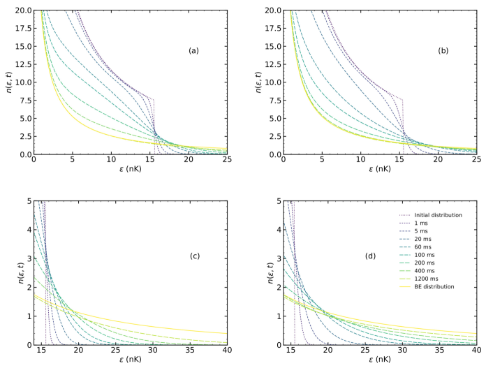
Contrary to the case of constant transport coefficients, the NBDE (5) for energy-dependent transport coefficients is not known to be solvable via a nonlinear transformation, a numerical solution is required. The library for scientific machine learning of the programming language Julia offers a wide range of computationally strong algorithms to deal with nonlinear partial differential equations [19]. For Julia v1.6.7, the package MethodOfLines v0.10.0 was used for a finite difference discretization of a symbolically defined partial differential equation. The method of lines (MOL) discretization is a scheme in which all but one dimension are discretized [20]. The differential equation is reduced to a single continuous dimension, and hence the solution can be computed via methods of numerical integration of ordinary differential equations. The computations shown in Fig. 2 (b,d) and Fig. 3 are done for a domain and with boundaries , and , where is a quenched Bose–Einstein distribution.
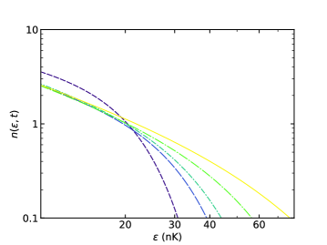
Comparing the UV tail of the numerical solution with energy-dependent transport coefficients in Fig. 2 (b,d) to the analytical solution [7, 8] of the nonlinear diffusion model with constant transport coefficients in Fig. 2 (a,c), or in the double-log-scale of Fig. 3, a significantly faster thermalization for energies occurs in the energy-dependent case, as required. The temporal dynamics of the distribution function for energies smaller than the quench-energy does not change significantly with energy-dependent coefficients. For times larger than the system is assumed to be in equilibrium since it has reached twice the experimental thermalization value of .
There appear, however, two numerical artifacts due to the fact that the calculations are done on a finite and discrete map. Since the value for infinity can only be covered by a very large but finite number, the boundary is not equivalent to the pole of the analytical and equilibrium solution. Therefore, a small deviation of the numerical solution compared to the equilibrium solution occurs at . Secondly, because of the limited energy domain and the fixed boundary , the numerical solution is forced to drop, while the equilibrium solution has a non-zero thermal tail over the whole energy domain. Hence, even at there is still a small deviation between numerical and thermal tail. Nevertheless, using the numerical solution for the energy-dependent drift and diffusion yields an improved thermalization of the UV tail, and no overshoot when calculating the condensate fraction, see Sect. IV.
For constant coefficients, the numerical solution coincides with the exact analytical result when plotted together, apart from the two above-mentioned small IR and UV artifacts that would appear in any numerical solution. At 10 nK, exact and numerical solutions agree within four decimal places in the 39K case with the Julia solution. We had previously obtained corresponding agreements for 23Na with MATLAB [10] and 39K using C++ [8].
III.3 Time-dependent chemical potential
To determine the occupation of the condensed state , one requires particle-number conservation, which is a necessary condition for condensate formation to occur. Up to this point, we have assumed a fixed chemical potential in our model calculations. Setting the chemical potential to zero instead of will ensure a description of the system right when a condensate starts to form in overoccupied systems, without taking into account the initiation time that is needed for the chemical potential to reach the point of the phase transition. In contrast to relativistic systems where particles can emerge from the available energy, cold bosonic gases strictly adhere to particle-number conservation. This conservation principle can be enforced by adjusting the chemical potential for each timestep until it reaches zero.
The particle number of the thermal cloud for a distribution function with a time-dependent chemical potential is given by
| (24) |
where the density of states for a three-dimensional Bose gas in a box is given by with , as obtained from the substitution of a summation over the quantum numbers of the associated states with an energy integration [21]. For a harmonic oscillator potential the dependence is .
At each timestep, is determined to maintain particle number conservation, ensuring , until reaches zero and condensation starts. Any further difference between and is then attributed to the condensate [10], such that
| (25) |
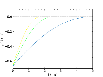
The concept of a time-dependent chemical potential is, however, questionable, since the distribution function for is not in equilibrium. Hence, it does not come as a surprise that the condensate initiation time for 39K vapor calculated from the numerical solution with energy-dependent transport coefficients as shown in Fig. 4 using particle-number conservation at each timestep comes out to be too small when compared to data. As an example, for 39K and a scattering length , the calculation yields ms, which is significantly larger than a result obtained using constant transport coefficients, but still smaller than the experimental value of [5]. The improvement is due to the fact that the thermalization of the tail of the distribution is faster and hence the constraint of particle-number conservation requires a slower adjustment of the chemical potential under the temporal dynamics of the nonlinear model. The large values for found experimentally may be due to slow ergodic mixing of the trapped atomic cloud [3] which is not explicitly taken into account in our model. For evaporative cooling in 87Rb at values of , measured initiation times [3] were found to agree with the results of a numerical model [22] based on quantum kinetic theory, but we are not aware of calculations for in a deep-quench situation as in [5] with . Hence, in the following we shall use the experimental values for when comparing to data, keeping their scaling with as shown in Table 1 and in Fig. 5.
In our semiclassical description, the initiation time approaches zero for very large scattering length , whereas in a quantum model a small finite limit should be approached, as could probably be tested in experiments with small atoms such as 7Li at very large scattering lengths. The initiation time diverges for , meaning that no condensate forms in a noninteracting system.
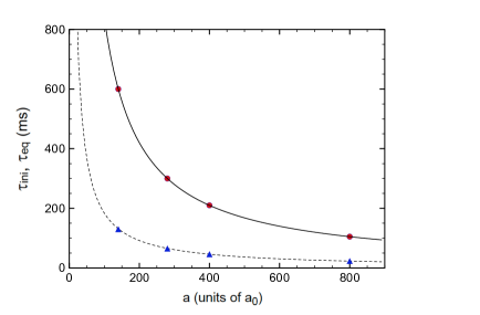
Regarding the scattering-length dependence of the equilibration times , in our previous investigation with constant transport coefficients for 39K [8] these were also taken to depend on in line with the experimentally determined scaling [5], and we keep this dependence in the present calculation for energy-dependent transport coefficients, see Fig. 5, upper solid curve. Whereas it may have been expected that the thermalization time depends on the inverse cross section [23] – and the transport coefficients on the cross section itself –, it has been shown that the dependence on the inverse interaction energies [13, 24] is due to the emerging coherence between the highly occupied infrared modes, see Davis et al. [25] for a summary.
The equilibration time diverges for vanishing interaction energy as expected, but the limit for it will have to be modified in a quantum description in order to remain larger than the initiation time. Such extremely large scattering lengths are, however, not reached in the present investigation: In the region , reasonable agreement with data is achieved for the time-dependent condensate fraction, see next section.
IV Time-dependent condensate formation
A numerical calculation of the time-dependent condensate fraction of 39K compared to the Cambridge data [5] is shown in Fig. 6. As and depend on the equilibration times, the scattering lengths , and the final temperature, respective pairs of energy-dependent transport coefficients were calculated with energy-averaged values according to Table 1 that are taken from our Ref. [8] for constant coefficients. The time-dependent transition to the condensate is obtained with the additional condition of particle-number conservation at each timestep, as explained in the previous section. Once the parameters for the case are fixed, no further adjustment is done since the time scales are proportional to and the transport coefficients are inversely related to the equilibration time.
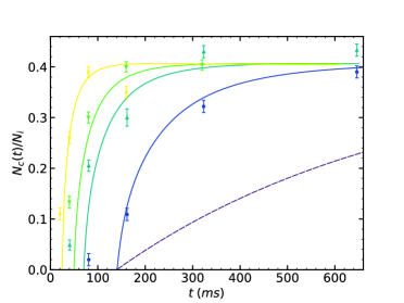
The NBDE-solutions with energy-dependent transport coefficients and the ensuing time-dependent (quasi-) condensate fractions are compared with the data [5] for various scattering lengths in Fig. 6. As in our previous work for constant coefficients [8], we focus on and 800. The values of the transport coefficients and their energy dependence have not been further optimized with respect to the Cambridge data at the individual scattering lengths in view of the relatively sparse data points that are presently available.
Condensation starts at the initiation time , and rises towards the equilibrium value . The rise is monotonic, no slight overshoot of the equilibrium value at large times occurs as may happen in the constant-coefficient case. However, in particular for , deviations in the short-time behavior are observed, because condensate formation in the model starts abruptly at the initiation time, whereas the 39K data may show a slow gradual increase, as had also been observed in the MIT 23Na data [1]. In contrast, the 87Rb condensate-formation data with slow evaporative cooling [3] start at the initiation time and have very small error bars there. Should precise future deep-quench data show a gradual increase, one would have to introduce time-dependent transport coefficients.
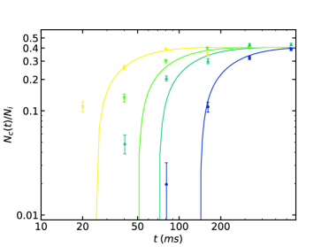
As in our previous model with constant transport coefficients [8], we confirm the experimental result [5] that the time-dependent condensate fractions for different scattering lengths fall on a single universal curve when plotted as functions of , before reaching the equilibrium limit for . Hence, the nonequilibrium system shows self-similar scaling [5], with a net flow of particles towards the infrared and into the condensed state. This is accompanied by a corresponding energy flow towards the ultraviolet carried by a small number of atoms that build up the Maxwell–Boltzmann tail, see Figs. 2 and 3.
A double-log plot of our NBDE-results for energy-dependent transport coefficients in Fig. 7 reveals that they obey power-law scaling only for very short times, whereas for intermediate times, they already bend over toward the equilibrium limit. Obviously, the index has to become time-dependent if one wants to use such laws to account for the time-dependent approach to equilibrium, as suggested in Ref. [5].
For a given initial distribution such as the truncated equilibrium distribution in the present work, an approximate solution of the equilibration problem can also be obtained through the linear relaxation ansatz that is sometimes used in descriptions of nonequilibrium problems, . It has the simple solution
| (26) |
which enforces equilibration towards the thermal distribution . When comparing the ensuing condensate fraction with the data, however, it turns out (see Fig. 6, dashed curve) that the relaxation ansatz fails to account for time-dependent condensate formation due to the neglect of the nonlinearity of the process, which is closely modeled by the NBDE.
The match between our results and the Cambridge data regarding the time-dependent condensate fraction shown in Figs. 6,7 is certainly not perfect, but it is way better than the outcome of a linear relaxation ansatz. The remaining discrepancy between our results and the data becomes particularly obvious in the double-log plot, Fig. 7. However, the general trend of the scattering-length-dependent data is well reproduced, and we expect that the agreement will improve once data with better time resolution become available. These are indeed available for 87Rb [3], but there for slow evaporative cooling, not for a deep quench that corresponds to the clean initial conditions that we are using here. Once deep-quench data with better time resolution become available, we shall aim for a proper -minimization of our results with respect to the data.
Regarding the requirement of energy conservation in the system, we note that it is the total energy that must be conserved, referring to the time-dependent mean-field term – see Eq. (1) – plus the collision term and therefore, the collision term as expressed by the NDBE need not conserve the energy by itself. In contrast, it does conserve the particle number once the particles that move into the condensed state are also considered. Hence, we have used it here to compute the time-dependent condensate fraction.
V Summary and Conclusions
We have modeled the thermalization and time-dependent condensate formation in a quenched Bose gas through solutions of the nonlinear boson diffusion equation. Concentrating on 39K where excellent Cambridge data are available, we have introduced energy-dependent drift and diffusion coefficients. This requires a numerical solution of the NBDE, which is performed using the Julia programming language. In the limiting case of constant diffusion coefficient and drift coefficient that we had previously solved analytically with deep-quench initial conditions and appropriate boundary conditions at the singularity through a nonlinear transformation, the numerical results for the time-dependent distribution functions are found to agree with the exact analytical results apart from small deviations in the IR and the UV that are due to the finite integration domain of the numerical approach.
The time-dependent condensate fraction is obtained through the additional condition of particle-number conservation following the quench that – in the particular 39K example – removes 77% of the atoms and 97.5% of the energy, reducing the temperature from nK to nK and eventually producing an equilibrium condensate fraction of . In the constant-coefficient case, the time-dependent approach of the condensate fraction to equilibrium may slightly overshoot the equilibrium value and later reach it from above, because a large constant drift towards the IR causes thermalization in the UV region to be too slow, such that at large times the Bose–Einstein limit is reached in the IR, but not yet in the UV. The resulting unbalanced energy-dependent equilibration has been remedied using energy-dependent drift and diffusion coefficients, requiring a numerical solution of the nonlinear diffusion equation.
In addition to particle-number conservation, the total energy must be conserved, referring to the time-dependent mean-field term plus the collision term. The collision term as expressed by the NDBE, however, need not conserve the energy by itself, although it does conserve the particle number once the particles that move into the condensed state are also considered. Hence, we have used it here to compute the time-dependent condensate fraction.
Agreement with the 39K data for the time-dependent condensate fraction at various scattering lengths is achieved, confirming the experimental result that the condensate initiation time and the equilibration time scale with the inverse scattering length. The nonlinearity in the collision term as modeled through the NBDE solutions thus turns out to be appropriate for an understanding of the BEC formation data, whereas results of the linear relaxation-time ansatz severely undercut the data for the time-dependent condensate fraction.
In the present cold-atom application of the nonlinear diffusion equation, we have thus improved the modeling through realistic energy-dependent transport coefficients instead of constant ones when comparing to the time-dependent condensate-formation data. There are other physical systems where the improvement is even more significant, so that the numerical solution method developed in this work will turn out to be useful.
This is particularly the case when the initial distribution is drastically different from the equilibrium one, as is the case for gluons in relativistic heavy-ion collisions: There, the initial nonequilibrium distribution of cold gluons is well approximated by a -function up to the gluon saturation momentum; it is very different from the thermal Bose–Einstein distribution and the momentum dependence of the transport coefficients should not be neglected. In the cold-atom case, the initial nonequilibrium distribution is already quite similar to the final B–E distribution in the IR, such that the energy dependence of the transport coefficients is less relevant in the IR, although necessary to overcome the unphysical UV features of the constant-coefficient case.
Acknowlegements
ML thanks Johannes Hölck for his help regarding the Julia code that has been developed for this work. We are grateful to Thomas Gasenzer for discussions and remarks.
References
- Miesner et al. [1998] H.-J. Miesner, D. M. Stamper-Kurn, M. R. Andrews, D. S. Durfee, S. Inouye, and W. Ketterle, Bosonic stimulation in the formation of a Bose-Einstein condensate, Science 279, 1005 (1998).
- Bijlsma et al. [2000] M. J. Bijlsma, E. Zaremba, and H. T. C. Stoof, Condensate growth in trapped Bose gases, Phys. Rev. A 62, 063609 (2000).
- Köhl et al. [2002] M. Köhl, M. J. Davis, C. Gardiner, T. Hänsch, and T. Esslinger, Growth of Bose-Einstein condensates from thermal vapor, Phys. Rev. Lett. 88, 080402 (2002).
- Gardiner et al. [1997] C. W. Gardiner, P. Zoller, R. J. Ballagh, and M. J. Davis, Kinetics of Bose-Einstein condensation in a trap, Phys. Rev. Lett. 79, 1793 (1997).
- Glidden et al. [2021] J. A. P. Glidden, C. Eigen, L. H. Dogra, T. A. Hilker, R. P. Smith, and Z. Hadzibabic, Bidirectional dynamic scaling in an isolated Bose gas far from equilibrium, Nature Phys. 17, 457 (2021).
- Wolschin [2018] G. Wolschin, Equilibration in finite Bose systems, Physica A 499, 1 (2018).
- Wolschin [2022] G. Wolschin, Nonlinear diffusion of fermions and bosons, EPL 140, 40002 (2022).
- Kabelac and Wolschin [2022] A. Kabelac and G. Wolschin, Time-dependent condensation of bosonic potassium, Eur. Phys. J. D 76, 178 (2022).
- Rasch and Wolschin [2020] N. Rasch and G. Wolschin, Solving a nonlinear analytical model for bosonic equilibration, Phys. Open 2, 100013 (2020).
- Simon and Wolschin [2021] A. Simon and G. Wolschin, Time-dependent condensate fraction in an analytical model, Physica A 573, 125930 (2021).
- Grangé et al. [1981] P. Grangé, H. A. Weidenmüller, and G. Wolschin, Beyond the TDHF: A collision term from a random-matrix model, Annals Phys. 136, 190 (1981).
- Snoke and Wolfe [1989] D. W. Snoke and J. P. Wolfe, Population dynamics of a Bose gas near saturation, Phys. Rev. B 39, 4030 (1989).
- Kagan et al. [1992] Y. M. Kagan, B. V. Svistunov, and G. V. Shlyapnikov, Kinetics of Bose condensation in an interacting Bose gas, Sov. Phys. JETP 74, 279 (1992).
- Semikoz and Tkachev [1995] D. V. Semikoz and I. I. Tkachev, Kinetics of Bose condensation, Phys. Rev. Lett. 74, 3093 (1995).
- Luiten et al. [1996] O. J. Luiten, M. W. Reynolds, and J. T. M. Walraven, Kinetic theory of the evaporative cooling of a trapped gas, Phys. Rev. A 53, 381 (1996).
- Holland et al. [1997] M. Holland, J. Williams, and J. Cooper, Bose-Einstein condensation: Kinetic evolution obtained from simulated trajectories, Phys. Rev. A 55, 3670 (1997).
- Jaksch et al. [1997] D. Jaksch, C. W. Gardiner, and P. Zoller, Quantum kinetic theory. II. Simulation of the quantum Boltzmann master equation, Phys. Rev. A 56, 575 (1997).
- Grossmann and Holthaus [1995] S. Grossmann and M. Holthaus, On Bose-Einstein condensation in harmonic traps, Phys. Lett. A 208, 188 (1995).
- Rackauckas and Nie [2017] C. Rackauckas and Q. Nie, Differentialequations.jl, a performant and feature-rich ecosystem for solving differential equations in Julia, J. Open Res. Software 5, 15 (2017).
- Schiesser [1991] W. E. Schiesser, The numerical method of lines: Integration of partial differential equations (Academic Press, San Diego, 1991).
- Pitaevskii and Stringari [2016] L. Pitaevskii and S. Stringari, Bose-Einstein condensation and superfluidity, Vol. 164 (Oxford University Press, 2016).
- Davis et al. [2000] M. J. Davis, C. Gardiner, and R. J. Ballagh, Quantum kinetic theory. VI. the influence of vapor dynamics on condensate growth, Phys. Rev. A 62, 063608 (2000).
- Stoof [1991] H. T. C. Stoof, Formation of the condensate in a dilute Bose gas, Phys. Rev. Lett. 66, 3148 (1991).
- Svistunov [1991] B. V. Svistunov, Highly nonequilibrium Bose condensation in a weakly interacting gas, J. Mosc. Phys. Soc. 1, 373 (1991).
- Davis et al. [2017] M. J. Davis, T. M. Wright, T. Gasenzer, S. A. Gardiner, and N. P. Proukakis, Formation of Bose–Einstein condensates, in Universal themes of Bose-Einstein condensation, Cambridge University Press (eds. N. P. Proukakis et al.) (2017).