Multi-Source and Test-Time Domain Adaptation on Multivariate Signals using Spatio-Temporal Monge Alignment

Abstract

Machine learning applications on signals such as computer vision or biomedical data often face significant challenges due to the variability that exists across hardware devices or session recordings. This variability poses a Domain Adaptation (DA) problem, as training and testing data distributions often differ. In this work, we propose Spatio-Temporal Monge Alignment (STMA) to mitigate these variabilities. This Optimal Transport (OT) based method adapts the cross-power spectrum density (cross-PSD) of multivariate signals by mapping them to the Wasserstein barycenter of source domains (multi-source DA). Predictions for new domains can be done with a filtering without the need for retraining a model with source data (test-time DA). We also study and discuss two special cases of the method, Temporal Monge Alignment (TMA) and Spatial Monge Alignment (SMA). Non-asymptotic concentration bounds are derived for the mappings estimation, which reveals a bias-plus-variance error structure with a variance decay rate of $\mathcal{O}(n_{\ell}^{-1/2})$ with $n_{\ell}$ the signal length. This theoretical guarantee demonstrates the efficiency of the proposed computational schema. Numerical experiments on multivariate biosignals and image data show that STMA leads to significant and consistent performance gains between datasets acquired with very different settings. Notably, STMA is a pre-processing step complementary to state-of-the-art deep learning methods.

1 Introduction

Machine learning approaches have led to impressive results across many applications, from computer vision and biology to audio and language processing. However, these approaches have known limitations in the presence of distribution shifts between training and evaluation datasets. Indeed, performance drops in the presence of distribution shifts have been observed in different fields such as computer vision [1], clinical data [2], and tabular data [3].

Domain Adaptation (DA) from single to multi-domain

This problem of data shift is well-known in machine learning and has been investigated in the DA community [4, 5, 6, 7]. Given source domain data with access to labels, DA methods aim to learn a model that can adequately predict on a target domain where no label is available, assuming the existence of a distribution shift between the two domains. Traditionally, DA methods try to adapt the source to be closer to the target using reweighting methods [4, 8], mapping estimation [9, 10] or dimension reduction [11]. Inspired by the successes of deep learning in computer vision, modern methods aim to reduce the shift between the embeddings of domains learned by a feature extractor. To achieve this, most methods attempt to minimize a divergence between the features of the source and target data. Several divergences have been proposed in the literature: correlation distance [12], adversarial method [1], maximum mean discrepancy distance [13] or Optimal Transport (OT) [14, 15].

With the rise of portable devices and open data, the problem of DA has evolved from a single-source setting where only one source is known to a multi-source setting where each source domain can have a different shift. This leads to a multi-source DA problem [16], where the variability across multiple domains can help training better predictors. For instance, one can learn domain-specific batch normalization [17, 18], compute weights to give more importance to some domains [19], or use moment matching to align the features [20]. Another method to deal with multiple sources is to create an intermediate domain between sources and target. [21] propose to compute a Wasserstein barycenter of the sources and then project this barycenter to the target using classical OT methods.

An additional challenge with traditional DA methods [15, 1, 12] is that they require using both the source and target domains to train the predictor. This means one needs access to the source data to train a model for new domains. However, the source data may not always be available due to privacy concerns or memory limitations. Test-time DA is a branch of DA that aims to adapt a predictor to the target data without access to the source data. In [22], the authors propose SHOT, which trains the classifier on source data and matches the target features to the fixed classifier using Information Maximization (IM). IM aims to produce predictions that are individually confident and globally diverse. [23] enhance SHOT with multi-source information, allowing the selection of the optimal combination of sources by learning the weights of each source model. [24] uses the local structure clustering technique on the target feature to adapt the model. Note that these methods are often complex and require high computational resources since they require training a new estimator for each new target domain.

DA for multivariate signals and biomedical data

This paper focuses on multi-source and test-time DA for multivariate signals, which are common in applications where data is collected from multiple devices. For instance, in the biomedical field, signals such as Electroencephalogram (EEG), Electrocardiogram (ECG), or Electromyogram (EMG) are often multivariate and can exhibit a shift between subjects, sessions, or devices. Several applications of DA in biosignals have been proposed for pairs of datasets [25, 26]. However, in clinical datasets, we often have access to multiple subjects or hospital data, which can be considered as separate domains. In this paper, we are interested in two biosignal applications with their own specificities: sleep staging and Brain-Computer Interface (BCI). Sleep staging is the process of categorizing sleep into five stages based on the electrical activity of the brain, i.e., EEG [27]. BCI motor imagery classifies mental visualization of motor movements using EEG signals. In both applications, datasets can exhibit diverse population distributions because of variations in factors such as age, gender, diseases, or individual physiological responses to stimuli [28]. All these variabilities introduce data shifts between different subjects or datasets (domains) that limit performances of traditional supervised learning methods [29, 26].

To take into account those shifts, or more precisely to try to mitigate them, simple normalization techniques have proven useful for BCI and sleep staging, leading to easy computation and application at test-time. For instance, researchers proposed Riemannian Procrustes Analysis (RPA) [30] to reduce the shift in BCI. RPA matches data distributions of source and target domains through recentering, stretching, and rotation, while operating on a Riemanian manifold of covariance matrices. When using deep learning, people typically only use the recentering part proposed in RPA and recenter the signal using Euclidean alignment [31, 32] or Riemannian Alignment (RA) [33, 29]. Alternatively, in sleep staging, a study by [34] utilized a convolutional Monge mapping normalization method to align each signal to a Wasserstein barycenter. This approach improved sleep staging significantly, compared to classical normalization techniques, such as the unit standard deviation scaling [35, 36].

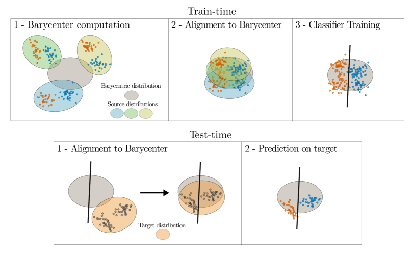
Figure 1: Illustration of Monge Alignment. At train-time the barycenter (grey ellipse) is estimated from 3 source distributions (colored ellipses). The predictor is learned on normalized data. At test-time the same barycenter is used to align the unlabeled target distribution (orange ellipse) and predict.

Contributions

This paper proposes a general method for multi-source and test-time DA for multivariate signals. This method denoted as Monge Alignment (MA), uses OT modeling of stationary signals to estimate a mapping. The latter aligns the different domains onto a barycenter of the domains before learning a predictor, attenuating the shift (Figure 1 top). At test time, one only needs to align the target domain on the barycenter and predict with the trained model (Figure 1 bottom). This method can be seen as a special case of [21], where the authors propose to align signals using the Wasserstein barycenter, but where the modeling of multivariate signals allows for more efficient barycenter computation and mapping estimation. It is also a generalization of the preliminary work of [34] where a Convolutional Monge Mapping Normalization was proposed to deal very efficiently with temporal shifts, but the different signals in the observations are assumed to be independent. The novel contributions of this paper are:

• A general method for multi-source and test-time DA for multivariate signals, using OT between Gaussian signals, denoted as Spatio-Temporal Monge Alignment (STMA) as well as Temporal and Spatial Monge Alignments (TMA and SMA respectively) tailored for specific shifts assumptions.

• Efficient algorithms for estimations of the mapping and the barycenter of the signals using Fast Fourier Transform (FFT) and block-diagonalization of the covariances matrices.

• Non-asymptotic concentration bounds of STMA, TMA and SMA estimation which present the interactions between the number of samples, the number of domains, the dimensionality of the signals, and the size of the filters.

• Novel numerical experiments on two biosignal tasks, Sleep staging, and BCI motor imagery, that show the benefits of the proposed method over state-of-the-art methods and illustrate the relative importance of spatial and temporal filtering.

In addition to the contributions discussed above, the proposed multi-source method is predictor-agnostic. It can be used for shallow or deep learning methods, as it acts as a pre-processing step. The estimated parameters can be very efficiently computed for new domains without the need for the source data or refitting of the learned model at test-time. Table 1 summarizes the specificities of the proposed method compared to other existing DA methods.

Paper outline

After quickly recalling OT between Gaussian distributions, we introduce the spatio-temporal Monge mapping for Gaussian multivariate signals in subsection 3.1. In section 4, we detail the Spatio-Temporal Monge Alignment (STMA) method for multi-source and test-time DA and its special cases using only temporal (TMA) or spatial (SMA) alignments. This section also provides non-asymptotic concentration bounds which reveals a bias-plus-variance error structure. In section 5, we apply MA to two real-life biosignal tasks using EEG data: sleep stage classification and BCI motor imagery and provide an illustrative example on images (2D signals).

Methods	Multi-source	Test-time	No need to refit	Method agnostic	Temporal shift	Spatial shift
Divergence minimization [12]	✗	✗	✗	✗	✓	✓
Moment Matching [20]	✓	✗	✗	✗	✓	✓
SHOT [22]	✗	✓	✗	✗	✓	✓
DECISION [23]	✓	✓	✗	✗	✓	✓
AdaBN [17]	✓	✓	✓	✗	✓	✓
Riemanian Alignment [29]	✓	✓	✓	✓	✗	✓
Temporal MA [34]	✓	✓	✓	✓	✓	✗
Spatial MA (ours)	✓	✓	✓	✓	✗	✓
Spatio-Temp MA (ours)	✓	✓	✓	✓	✓	✓

Table 1: Comparison of DA methods with various specificities. “Multi-source indicates the ability to handle multiple sources, “Test-time” means that the method does not require source data at test-time, “No need to refit” signifies whether refitting is required for a new domain at test-time, “Method agnostic” refers to independence from a specific type of predictors (e.g., deep learning), while “Temporal shift” and “Spatial shift” indicate the capability to handle temporal and spatial shifts. Only STMA handles all the specificities.

Notations

Vectors are denoted by small cap boldface letters (e.g., $\mathbf{x}$), matrices by large cap boldface letters (e.g., $\mathbf{X}$). The element-wise product is $\odot$, and the element-wise power of $n$ is $\cdot^{\odot n}$. $\left\llbracket 1,K\right\rrbracket\,$ denotes $\{1,\ldots,K\}$. The absolute value is $|.|$. The discrete convolution operator is $*$. $\mathcal{S}_{n}$ and $\mathcal{S}_{n}^{++}$ denote the sets of symmetric and symmetric positive definite matrices of size $n\times n$. $\mathcal{H}_{n}$ and $\mathcal{H}_{n}^{++}$ denote the sets of hermitian and hermitian positive definite matrices of size $n\times n$. $\mathcal{C}_{n}$ is the set of real-valued circulant matrices of size $n\times n$. We denote by $\lambda_{\max}(\mathbf{A})$ the maximum eigenvalue of the matrix $\mathbf{A}$. We also define the effective rank by $\mathbf{r}(\mathbf{A})=\frac{\text{tr}(\mathbf{A})}{\lambda_{\max}(\mathbf{A})}$ where $\text{tr}(\mathbf{A})$ is the trace of $\mathbf{A}$. $\mathbb{N}^{*}$ is the integer set excluding $0$, and $\mathbb{R}^{+*}$ is the set of strictly positive real values. $\mathbf{X}_{k}$ and $\mathbf{X}_{t}$ relate to source domains $k\in\left\llbracket 1,n_{d}\right\rrbracket\,$ and the target domain, respectively. $\operatorname{vec}:\mathbb{R}^{n_{c}\times n_{\ell}}\to\mathbb{R}^{n_{c}n_{\ell}}$ concatenates rows of a time series into a vector, and $\operatorname{vec}^{-1}:\mathbb{R}^{n_{c}n_{\ell}}\to\mathbb{R}^{n_{c}\times n_{\ell}}$ is the reciprocal. $\left\lceil{.}\right\rceil$ and $\left\lfloor{.}\right\rfloor$ denote the smallest integer greater than or equal to, and the greatest integer less than or equal to, respectively. $(\mathbf{x})_{l}$ refers to the $l^{\text{th}}$ element of $\mathbf{x}$, and $(\mathbf{X})_{lm}$ denotes the element of $\mathbf{X}$ at the $l^{\text{th}}$ row and $m^{\text{th}}$ column. $\mathbf{X}^{\mathsf{H}}$ is the conjugate transpose of $\mathbf{X}$. $\otimes$ is the Kronecker operator.

2 Signal adaptation with Optimal Transport

In this section, we first briefly introduce OT between centered Gaussian distributions. Then, we describe how [34] has used this mapping between distributions to align univariate signals on a barycenter. Finally, we introduce approximations on circulant matrices, which explain how the structure of covariance matrices is efficiently used.

2.1 Optimal Transport between Gaussian distributions

2.1.1 Monge mapping for Gaussian distributions

Let two Gaussian distributions $\mu_{s}=\mathcal{N}(\mathbf{0},{\boldsymbol{\Sigma}}_{s})$ and $\mu_{t}=\mathcal{N}(\mathbf{0},{\boldsymbol{\Sigma}}_{t})$, where ${\boldsymbol{\Sigma}}_{s}$ and ${\boldsymbol{\Sigma}}_{t}$ are symmetric positive definite matrices. OT between Gaussian distributions is one of the rare cases where a closed-form solution exists.

The OT mapping, also called Monge mapping, is the following affine function [37, 38, 39]:

$$m(\mathbf{x})=\mathbf{A}\mathbf{x}\quad\text{with}\quad\mathbf{A}={\boldsymbol{\Sigma}}_{s}^{-\frac{1}{2}}\left({\boldsymbol{\Sigma}}_{s}^{\frac{1}{2}}{\boldsymbol{\Sigma}}_{t}{\boldsymbol{\Sigma}}_{s}^{\frac{1}{2}}\right)^{\frac{1}{2}}{\boldsymbol{\Sigma}}_{s}^{-\frac{1}{2}}=\mathbf{A}^{\mkern-1.5mu\mathsf{T}}\;.$$ (1)

In practical applications, one can estimate the covariance matrices of the two distributions to get an estimation of the Wasserstein distance and its associated mapping [40].

2.1.2 Wasserstein barycenter between Gaussian distributions

The Wasserstein barycenter $\overline{\mu}$ defines a notion of averaging of probability distributions $\{\mu_{k}\}_{1\leq k\leq n_{d}}$ which is the solution of a convex program involving Wasserstein distances:

$$\overline{\mu}\triangleq\underset{\mu}{\text{arg min}}\;\frac{1}{n_{d}}\sum_{k=1}^{n_{d}}\mathcal{W}_{2}^{2}(\mu,\mu_{k})\;.$$ (2)

Interestingly, when $\mu_{k}$ are Gaussian distributions, the barycenter is still a Gaussian distribution $\overline{\mu}=\mathcal{N}(\mathbf{0},\overline{{\boldsymbol{\Sigma}}})$ [41]. There is, in general, no closed-form expression for computing the covariance matrix $\overline{{\boldsymbol{\Sigma}}}$. But the first order optimality condition of this convex problem shows that $\overline{{\boldsymbol{\Sigma}}}$ is the unique positive definite fixed point of the map

$$\overline{{\boldsymbol{\Sigma}}}=\Psi\left(\overline{{\boldsymbol{\Sigma}}},\left\{{\boldsymbol{\Sigma}}_{k}\right\}_{k=1}^{n_{d}}\right)\quad\text{where}\quad\Psi\left(\mathbf{A},\left\{\mathbf{B}_{k}\right\}_{k=1}^{n_{d}}\right)=\frac{1}{n_{d}}\sum_{k=1}^{n_{d}}\left(\mathbf{A}^{\frac{1}{2}}\mathbf{B}_{k}\mathbf{A}^{\frac{1}{2}}\right)^{\frac{1}{2}}.$$ (3)

Iterating this fixed-point map, i.e.,

$$\overline{{\boldsymbol{\Sigma}}}^{(\ell+1)}=\Psi\left(\overline{{\boldsymbol{\Sigma}}}^{(\ell)},\left\{{\boldsymbol{\Sigma}}_{k}\right\}_{k=1}^{n_{d}}\right),$$ (4)

converges in practice to the solution $\overline{{\boldsymbol{\Sigma}}}$ [42].

2.2 OT mapping of stationary signals using circulant matrices

OT emerges as a natural tool for addressing distribution shift and has found significant application in DA, as evidenced by works such as [43], [15], and [19]. Another line of methods leverages the Gaussian assumption to computationally simplify the estimation of Wasserstein mapping and barycenter, as illustrated in [42] and [40]. In the context of this work, the focus is on the analysis of time-series data. Under certain judicious assumptions, the computational efficiency of Monge mapping and barycenter computation is further enhanced, as proposed by [34].

2.2.1 Circulant matrices for stationary and periodic signals

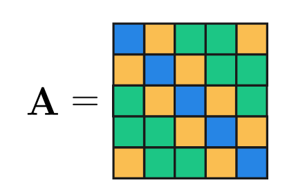
(a) $\mathbf{A}\in{\mathcal{C}_{5}\cap\mathcal{S}_{5}^{++}}$ with coefficients $\color[rgb]{0.1484375,0.5234375,0.8984375}\mdblksquare\color[rgb]{0,0,0},\color[rgb]{0.98046875,0.74609375,0.31640625}\mdblksquare\color[rgb]{0,0,0},\color[rgb]{0.109375,0.77734375,0.5234375}\mdblksquare\color[rgb]{0,0,0}\in\mathbb{R}$

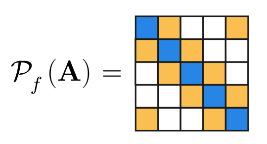
(b) $\mathcal{P}_{f}(\mathbf{A})\in{\mathcal{E}_{3,5}\cap\mathcal{S}_{5}^{++}}$ approximates $\mathbf{A}$

Figure 2: A Monge mapping $\mathbf{A}$ (cf. Equation 1) that is a $5\times 5$ symmetric positive definite and circulant matrix, i.e., belonging to $\mathcal{C}_{5}\cap\mathcal{S}_{5}^{++}$, and its approximation in $\mathcal{E}_{3,5}\cap\mathcal{S}_{5}^{++}$ as defined in Equation 9. In this case, for $\mathbf{x}\in\mathbb{R}^{n_{\ell}}$, $\mathcal{P}_{f}(\mathbf{A})\mathbf{x}=\mathbf{h}*\mathbf{x}$ with $\mathbf{h}=[\color[rgb]{0.98046875,0.74609375,0.31640625}\mdblksquare\color[rgb]{0.1484375,0.5234375,0.8984375}\mdblksquare\color[rgb]{0.98046875,0.74609375,0.31640625}\mdblksquare\color[rgb]{0,0,0}]^{\mkern-1.5mu\mathsf{T}}$.

A common assumption in signal processing is that if the signal is long enough, then the signal can be considered periodic and stationary, and the covariance matrix becomes a symmetric positive definite (i.e., $\mathcal{S}_{n_{\ell}}^{++}$) and circulant (i.e., $\mathcal{C}_{n_{\ell}}$) matrix i.e., a symmetric positive definite matrix with cyclically shifted rows. 2(a) presents an example of such a matrix with an univariate signal of length $n_{\ell}=5$. The utility of this assumption lies in its diagonalization through the Fourier basis, simplifying analyses and computations on such time series. Indeed, for $\mathbf{A}\in{\mathcal{C}_{n_{\ell}}\cap\mathcal{S}_{n_{\ell}}^{++}}$ and denoting the power spectrum density (PSD) by $\mathbf{q}\in(\mathbb{R}^{+*})^{{n_{\ell}}}$, we have the decomposition [44, Theorem 3.1]

$$\mathbf{A}=\mathbf{F}_{n_{\ell}}\operatorname{diag}(\mathbf{q})\mathbf{F}_{n_{\ell}}^{\mathsf{H}}\;,$$ (5)

with the Fourier basis of elements

$$(\mathbf{F}_{n_{\ell}})_{lm}\triangleq\frac{1}{\sqrt{n_{\ell}}}\exp\left(-2i\pi\frac{(l-1)(m-1)}{n_{\ell}}\right)\;,$$ (6)

for $l,m\in\left\llbracket 1,n_{\ell}\right\rrbracket\,$ and $n_{\ell}\in\mathbb{N}^{*}$.

2.2.2 Convolutional Monge Mapping and filter size

In the paper by [34], the authors use the circularity structure to diagonalize all the covariance matrices with the Fourier basis. This leads to a simplification of the Monge mapping Equation 1. Let us consider two centered Gaussian distributions: a source distribution $\mathcal{N}(\mathbf{0},{\boldsymbol{\Sigma}}_{s})$ and a target distribution $\mathcal{N}(\mathbf{0},{\boldsymbol{\Sigma}}_{t})$, both with covariance matrices in $\mathcal{C}_{n_{\ell}}\cap\mathcal{S}_{n_{\ell}}^{++}$, and a realization $\mathbf{x}\in\mathbb{R}^{n_{\ell}}$ of the source distribution. Using Fourier-based eigen-factorization of the covariance matrices, we can map between these two Gaussian distributions, characterized by their power spectral densities (PSDs) $\mathbf{q}_{s}\triangleq\operatorname{diag}(\mathbf{F}_{n_{\ell}}^{\mathsf{H}}{\boldsymbol{\Sigma}}_{s}\mathbf{F}_{n_{\ell}})$ and $\mathbf{q}_{t}\triangleq\operatorname{diag}(\mathbf{F}_{n_{\ell}}^{\mathsf{H}}{\boldsymbol{\Sigma}}_{t}\mathbf{F}_{n_{\ell}})$, with the Monge mapping from Equation 1. This mapping $\mathbf{A}$ belongs to $\mathcal{C}_{n_{\ell}}\cap\mathcal{S}_{n_{\ell}}^{++}$ and hence can be expressed as the following convolution [44, Chapter 3]

$$m(\mathbf{x})=\mathbf{h}*\mathbf{x}\;,\quad\text{with}\quad\mathbf{h}\triangleq\frac{1}{\sqrt{n_{\ell}}}\mathbf{F}_{n_{\ell}}^{\mathsf{H}}\left(\mathbf{q}_{t}^{\odot\frac{1}{2}}\odot\mathbf{q}_{s}^{\odot-\frac{1}{2}}\right)\in\mathbb{R}^{n_{\ell}}\;.$$ (7)

Utilizing the same factorization, [34] introduce a novel closed-form expression for barycenter computation. Subsequently, the authors propose the Convolutional Monge Mapping Normalization (CMMN) method, wherein a barycenter is computed, and all domains are aligned to this central point, constituting a test-time DA approach. Notably, this method exhibits significant performance gains in practical applications.

A nuanced aspect of this technique lies in choosing the filter size in Equation 7. In practice, $\mathbf{h}$ is computed with a size $f$ instead of $n_{\ell}$. Opting for a filter size equivalent to the signal size (i.e., $f=n_{\ell}$) results in a perfect mapping of domains to the barycenter, potentially eliminating class-discriminative information. Selecting $f=1$ scales the entire signal, equivalent to a standard z-score operation. Despite its significance, the impact of $f$ is not studied by [34]. Here, we explore the approximations made to incorporate the filter size $f$ into the theoretical framework.

2.2.3 Approximation of circulant matrices

Matrices in $\mathcal{C}_{n_{\ell}}$, and their associated filter, have $n_{\ell}$ parameters, i.e., the signal length. To reduce this parameter number, we propose approximating matrices in $\mathcal{C}_{n_{\ell}}$ by linear mappings with only $f\ll n_{\ell}$ parameters. First, we define the set of circulant matrices with $f$ parameters as

$$\mathcal{E}_{f,n_{\ell}}\triangleq\left\{\mathbf{A}\in\mathcal{C}_{n_{\ell}}\mid(\mathbf{A})_{1l}=0,\;l\in\left\llbracket\left\lceil{f/2}\right\rceil+1,n_{\ell}-\left\lfloor{f/2}\right\rfloor\right\rrbracket\right\}\;.$$ (8)

Then, we approximate every $\mathbf{A}\in\mathcal{C}_{n_{\ell}}$ by its nearest element in $\mathcal{E}_{f,n_{\ell}}$, i.e.,

$$\mathcal{P}_{f}(\mathbf{A})\triangleq\mathop{\rm arg\,min}_{\mathbf{\Gamma}\in\mathcal{E}_{f,n_{\ell}}}\,\|\mathbf{\Gamma}-\mathbf{A}\|_{\text{Fro}}$$ (9)

where $\|.\|_{\text{Fro}}$ is the Frobenius norm. Thus, $\mathcal{P}_{f}(\mathbf{A})$ is the orthogonal projection of $\mathbf{A}$ onto $\mathcal{E}_{f,n_{\ell}}$ and its elements are $(\mathcal{P}_{f}(\mathbf{A}))_{1l}=(\mathbf{A})_{1l}$ for $l\in\left\llbracket 1,\left\lceil{f/2}\right\rceil\right\rrbracket\,\cup\llbracket n_{\ell}-\left\lfloor{f/2}\right\rfloor+1,n_{\ell}\rrbracket$. An example in $\mathcal{E}_{3,5}$ is presented in 2(b). With this approximation, we get that $\mathcal{P}_{f}(\mathbf{A})$ applies a convolution with the filter $\mathbf{h}\in\mathbb{R}^{f}$ that contains the non-zero elements of the first row of $\mathbf{A}$,

$$\mathcal{P}_{f}(\mathbf{A})\;\mathbf{x}=\mathbf{h}*\mathbf{x}\enspace.$$ (10)

Since $\mathcal{P}_{f}(\mathbf{A})\in\mathcal{C}_{n_{\ell}}$, it admits the decomposition $\mathcal{P}_{f}(\mathbf{A})=\mathbf{F}_{n_{\ell}}\operatorname{diag}(\mathbf{q})\mathbf{F}_{n_{\ell}}^{\mathsf{H}}$ with $\mathbf{q}\in\mathbb{C}^{n_{\ell}}$ that will be interpreted latter as a cross-PSD. An important property of $\mathbf{h}$ is its computation from a sub-sampling of $\mathbf{q}$, denoted $\mathbf{p}\in{\mathbb{C}^{f}}$ and of elements

$$(\mathbf{p})_{l}\triangleq(\mathbf{q})_{\frac{(l-1)n_{\ell}}{f}+1}$$ (11)

for $l\in\left\llbracket 1,f\right\rrbracket\,$. We denote by $g_{f}$ the function that does this operation, i.e.,

$$g_{f}(\mathbf{q})\triangleq\mathbf{p}\;.$$ (12)

The following proposition bridges the gap between filtering, $\mathcal{E}_{f,n_{\ell}}$ and $g_{f}$. This way, we can sub-sample a given cross-PSD to get a smaller one of size $f$. The associated filter is computed with an inverse Fourier transform and the mapping is achieved with a convolution. Overall, the number of parameters is $f$ and the complexity to compute the filter and the mapping are $\mathcal{O}(f\log(f))$ and $\mathcal{O}(n_{\ell}\log(n_{\ell}))$ respectively thanks to the Fast Fourier Transform (FFT).

Proposition 1 ($\mathcal{E}_{f,n_{\ell}}$ and filtering)

Let $\mathbf{F}_{n_{\ell}}\in\mathbb{C}^{n_{\ell}\times n_{\ell}}$ and $\mathbf{F}_{f}\in\mathbb{C}^{f\times f}$ be the Fourier bases. Given $\mathbf{A}=\mathbf{F}_{n_{\ell}}\operatorname{diag}(\mathbf{q})\mathbf{F}_{n_{\ell}}^{\mathsf{H}}\in\mathcal{E}_{f,n_{\ell}}$ with $\mathbf{q}\in\mathbb{C}^{n_{\ell}}$, and $\mathbf{h}\in\mathbb{R}^{f}$ the filter containing the non-zero elements of the first row of $\mathbf{A}$, then for every $\mathbf{x}\in\mathbb{R}^{n_{\ell}}$, we have

$$\mathbf{A}\mathbf{x}=\mathbf{h}*\mathbf{x}$$

where $*$ is the convolution operator and $\mathbf{h}$ is the inverse Fourier transform of $\mathbf{p}=g_{f}(\mathbf{q})\in{\mathbb{C}^{f}}$, i.e.,

$$\mathbf{h}=\frac{1}{\sqrt{f}}\mathbf{F}_{f}^{\mathsf{H}}\mathbf{p}\;.$$

3 Spatio-Temporal Monge mapping and barycenter for Gaussian signals

This section introduces a new method for mapping multivariate signals by seamlessly incorporating the filter size parameter and using the previously presented approximation of circulant matrices. We first describe the structure of the spatio-temporal covariance matrix. Then, we define the $f$-Monge mapping and compute its closed-form expression for the spatio-temporal structure as well as the associated Wasserstein barycenter. Next, we establish two mappings and their barycenters when only the temporal or spatial structure is considered. In the following, we consider multivariate signals $\mathbf{X}\triangleq[\mathbf{x}_{1},\dots,\mathbf{x}_{n_{c}}]^{\mkern-1.5mu\mathsf{T}}\in\mathbb{R}^{n_{c}\times n_{\ell}}$ with $n_{c}$ channels of length $n_{\ell}$, and assume that the vectorized signal follows a centered Gaussian distribution, i.e., $\operatorname{vec}(\mathbf{X})\sim\mathcal{N}(\mathbf{0},{\boldsymbol{\Sigma}})$ where ${\boldsymbol{\Sigma}}\in\mathcal{S}_{n_{c}n_{\ell}}^{++}$ is the spatio-temporal covariance matrix.

3.1 Spatio-temporal covariance matrix

First, the spatio-temporal covariance matrix is expressed as

$${\boldsymbol{\Sigma}}=\mathbb{E}\left[\operatorname{vec}(\mathbf{X})\operatorname{vec}(\mathbf{X})^{\mkern-1.5mu\mathsf{T}}\right]=\begin{pmatrix}{\boldsymbol{\Sigma}}_{1,1}&\dots&{\boldsymbol{\Sigma}}_{1,n_{c}}\\ \dots&\dots&\dots\\ {\boldsymbol{\Sigma}}_{n_{c},1}&\dots&{\boldsymbol{\Sigma}}_{n_{c},n_{c}}\end{pmatrix}\in\mathcal{S}_{n_{c}n_{\ell}}^{++}\;,$$ (13)

where ${\boldsymbol{\Sigma}}_{l,m}$ corresponds to the temporal covariance matrix between the signals of the l^th and the m^th channels. We add a simple assumption on the ${\boldsymbol{\Sigma}}_{l,m}$ that will lead to a simple Monge mapping later in this section.

Assumption 2

For every $l,m\in\left\llbracket 1,n_{c}\right\rrbracket\,^{2}$, we assume that ${\boldsymbol{\Sigma}}_{l,m}$, defined in Equation 13, belongs to $\mathcal{C}_{n_{\ell}}$, i.e.,

$${\boldsymbol{\Sigma}}_{l,m}=\mathbf{F}_{n_{\ell}}\operatorname{diag}(\mathbf{q}_{l,m})\mathbf{F}_{n_{\ell}}^{\mathsf{H}},$$

where $\mathbf{q}_{l,m}\in\mathbb{C}^{n_{\ell}}$ is such that the cross-PSD $\mathbf{Q}_{\ell}\triangleq\left[(\mathbf{q}_{l,m})_{\ell}\right]_{l,m=1,1}^{n_{c},n_{c}}\in\mathcal{H}_{n_{c}}^{++}$, for $\ell\in\left\llbracket 1,n_{\ell}\right\rrbracket\,$.

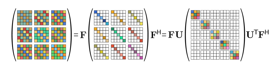
Figure 3: Block diagonalization of the covariance matrix ${\boldsymbol{\Sigma}}\in\mathcal{S}_{n_{c}n_{\ell}}^{++}$ following the Assumption 2 with $n_{\ell}=5$ and $n_{c}=3$. $\mathbf{F}=\operatorname{diag}(\mathbf{F}_{n_{\ell}},\dots,\mathbf{F}_{n_{\ell}})\in\mathbb{C}^{n_{c}n_{\ell}}$ and $\mathbf{U}$ is a permutation matrix.

Under the Assumption 2, ${\boldsymbol{\Sigma}}$ is re-written

$${\boldsymbol{\Sigma}}=\mathbf{F}\begin{pmatrix}\operatorname{diag}(\mathbf{q}_{1,1})&\dots&\operatorname{diag}(\mathbf{q}_{1,n_{c}})\\ \dots&\dots&\dots\\ \operatorname{diag}(\mathbf{q}_{n_{c},1})&\dots&\operatorname{diag}(\mathbf{q}_{n_{c},n_{c}})\end{pmatrix}\mathbf{F}^{\mathsf{H}}\;,$$ (14)

with $\mathbf{F}\triangleq\operatorname{diag}(\mathbf{F}_{n_{\ell}},\dots,\mathbf{F}_{n_{\ell}})\in\mathbb{C}^{n_{c}n_{\ell}\times n_{c}n_{\ell}}$. Hence, there exists a permutation matrix $\mathbf{U}\in\mathbb{R}^{n_{c}n_{\ell}\times n_{c}n_{\ell}}$ that block-diagonalizes ${\boldsymbol{\Sigma}}$, i.e.,

$${\boldsymbol{\Sigma}}=\mathbf{F}\mathbf{U}\mathbf{Q}\mathbf{U}^{\mkern-1.5mu\mathsf{T}}\mathbf{F}^{\mathsf{H}}\;,$$ (15)

with $\mathbf{Q}\triangleq\operatorname{diag}(\mathbf{Q}_{1},\dots,\mathbf{Q}_{n_{\ell}})\in{\mathcal{H}_{n_{c}n_{\ell}}^{++}}$ and $\mathbf{Q}_{\ell}$ defined in Assumption 2. An example of this decomposition for $n_{\ell}=5$ and $n_{c}=3$ is given in Figure 3. Notably, $\mathbf{Q}$ is the cross-PSD and can be sub-sampled by extending the function $g_{f}$ to block-diagonal matrices, i.e.,

$$g_{f}(\mathbf{Q})\triangleq\operatorname{diag}\left(\mathbf{Q}_{1},\mathbf{Q}_{\frac{n_{\ell}}{f}+1},\dots,\mathbf{Q}_{\frac{(f-1)n_{\ell}}{f}+1}\right)\in{\mathcal{H}_{n_{c}f}^{++}}.$$ (16)

Thus, we can sub-sample the cross-PSDs of the blocks of ${\boldsymbol{\Sigma}}$,

$$\begin{pmatrix}\operatorname{diag}(\mathbf{p}_{1,1})&\dots&\operatorname{diag}(\mathbf{p}_{1,n_{c}})\\ \dots&\dots&\dots\\ \operatorname{diag}(\mathbf{p}_{n_{c},1})&\dots&\operatorname{diag}(\mathbf{p}_{n_{c},n_{c}})\end{pmatrix}=\mathbf{V}g_{f}(\mathbf{Q})\mathbf{V}^{\mkern-1.5mu\mathsf{T}}\in{\mathcal{H}_{n_{c}f}^{++}}$$ (17)

with $\mathbf{p}_{l,m}=g_{f}(\mathbf{q}_{l,m})\in{\mathbb{C}^{f}}$ and $\mathbf{V}\in\mathbb{R}^{n_{c}f\times n_{c}f}$ a permutation matrix.

3.2 Spatio-Temporal $f$-Monge mapping and barycenter

The Assumption 2 implies a specific structure on the Monge mapping from Equation 1. Indeed, given $\mathcal{N}(\mathbf{0},{\boldsymbol{\Sigma}}_{s})$ and $\mathcal{N}(\mathbf{0},{\boldsymbol{\Sigma}}_{t})$ source and target centered Gaussian distributions respectively and following the Assumption 2, the Monge mapping, introduced in the Equation 1, has the structure

$$\mathbf{A}=\begin{pmatrix}\mathbf{A}_{1,1}&\dots&\mathbf{A}_{1,n_{c}}\\ \dots&\dots&\dots\\ \mathbf{A}_{n_{c},1}&\dots&\mathbf{A}_{n_{c},n_{c}}\end{pmatrix}\in\mathcal{S}_{n_{c}n_{\ell}}^{++}\quad\text{with}\quad\mathbf{A}_{l,m}\in\mathcal{C}_{n_{\ell}}$$

for every $l,m\in\left\llbracket 1,n_{c}\right\rrbracket\,$. This motivates the definition of the $f$-Monge mapping which leverages the approximation of circulant matrices defined in subsection 2.2.

Definition 3

Given $\mathcal{N}(\mathbf{0},{\boldsymbol{\Sigma}}_{s})$ and $\mathcal{N}(\mathbf{0},{\boldsymbol{\Sigma}}_{t})$ source and target centered Gaussian distributions respectively and following the Assumption 2, the $f$-Monge mapping on $\mathbf{X}\in\mathbb{R}^{n_{c}\times n_{\ell}}$ is defined as

$$m_{f}(\mathbf{X})=\operatorname{vec}^{-1}\left(\widetilde{\mathbf{A}}\operatorname{vec}\left(\mathbf{X}\right)\right)$$

where

$$\widetilde{\mathbf{A}}=\begin{pmatrix}\mathcal{P}_{f}(\mathbf{A}_{1,1})&\dots&\mathcal{P}_{f}(\mathbf{A}_{1,n_{c}})\\ \dots&\dots&\dots\\ \mathcal{P}_{f}(\mathbf{A}_{n_{c},1})&\dots&\mathcal{P}_{f}(\mathbf{A}_{n_{c},n_{c}})\end{pmatrix}\quad\text{and}\quad\mathbf{A}={\boldsymbol{\Sigma}}_{s}^{-\frac{1}{2}}\left({\boldsymbol{\Sigma}}_{s}^{\frac{1}{2}}{\boldsymbol{\Sigma}}_{t}{\boldsymbol{\Sigma}}_{s}^{\frac{1}{2}}\right)^{\frac{1}{2}}{\boldsymbol{\Sigma}}_{s}^{-\frac{1}{2}}$$

is the Monge mapping from Equation 1 and $\mathcal{P}_{f}$ is the function which sub-samples the cross-PSDs and defined in Equation 9.

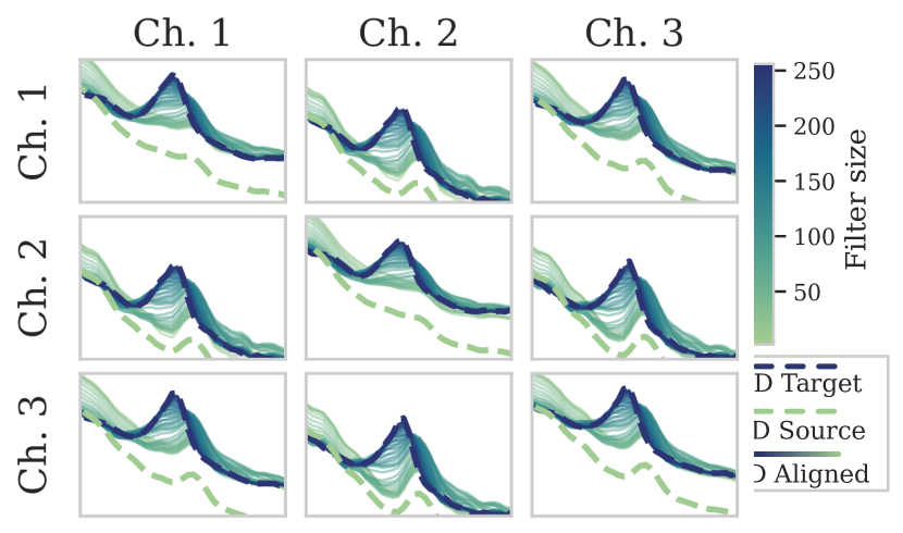
(a) Cross-PSD alignment

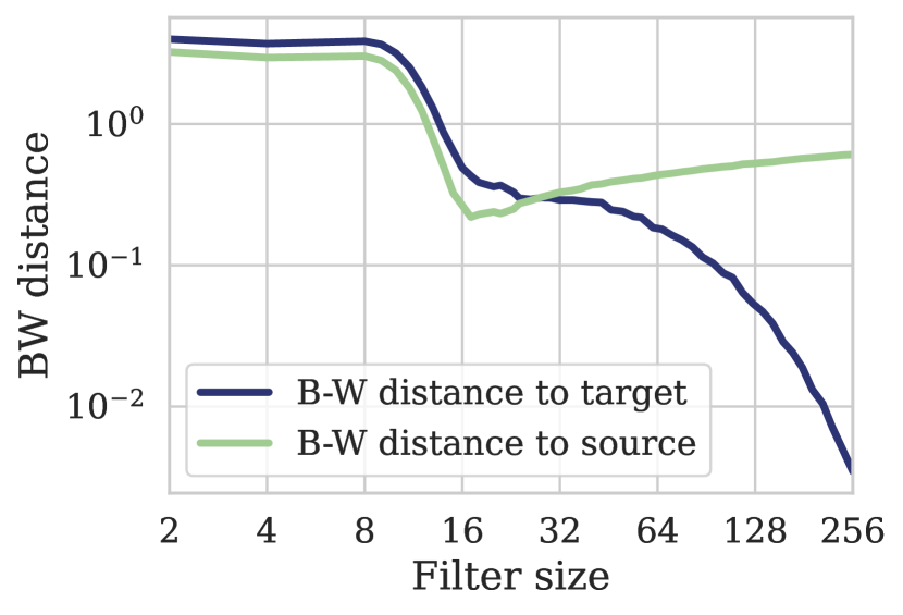
(b) Bures-Wasserstein distance

Figure 4: Illustration of the Spatio-Temporal Monge mapping on sleep data. (a) Cross-PSD alignment from source cross-PSD (green dotted line) to target cross-PSD (blue dotted line) for different filter sizes. (b) Bures-Wasserstein distance between the aligned signal and the source signal (green line) and the target line (blue line).

We now explore the properties of the $f$-Monge mapping. The next proposition establishes the spatio-temporal mapping, showing that it is a sum of convolutions and thus fast to compute.

Proposition 4 (Spatio-Temporal mapping)

Let $\mathcal{N}(\mathbf{0},{\boldsymbol{\Sigma}}_{s})$ and $\mathcal{N}(\mathbf{0},{\boldsymbol{\Sigma}}_{t})$ be source and target centered Gaussian distributions respectively and following the Assumption 2, i.e., for $d\in\{s,t\}$, ${\boldsymbol{\Sigma}}_{d}=\mathbf{F}\mathbf{U}\mathbf{Q}_{d}\mathbf{U}^{\mkern-1.5mu\mathsf{T}}\mathbf{F}^{\mathsf{H}}$ as defined in Equation 15. Let $f\leq n_{\ell}$, $\mathbf{P}_{d}=g_{f}(\mathbf{Q}_{d})$ and

$$\begin{pmatrix}\operatorname{diag}(\mathbf{p}_{1,1})&\dots&\operatorname{diag}(\mathbf{p}_{1,n_{c}})\\ \dots&\dots&\dots\\ \operatorname{diag}(\mathbf{p}_{n_{c},1})&\dots&\operatorname{diag}(\mathbf{p}_{n_{c},n_{c}})\end{pmatrix}\triangleq\mathbf{V}\mathbf{P}_{s}^{-\frac{1}{2}}\left(\mathbf{P}_{s}^{\frac{1}{2}}\mathbf{P}_{t}\mathbf{P}_{s}^{\frac{1}{2}}\right)^{\frac{1}{2}}\mathbf{P}_{s}^{-\frac{1}{2}}\mathbf{V}^{\mkern-1.5mu\mathsf{T}}\in{\mathcal{H}_{n_{c}f}^{++}}$$

with $\mathbf{V}\in\mathbb{R}^{n_{c}f\times n_{c}f}$ the permutation matrix from Equation 17. Given a signal $\mathbf{X}=[\mathbf{x}_{1},\dots,\mathbf{x}_{n_{c}}]^{\mkern-1.5mu\mathsf{T}}\in\mathbb{R}^{n_{c}\times n_{\ell}}$ such that $\operatorname{vec}(\mathbf{X})\sim\mathcal{N}(\mathbf{0},{\boldsymbol{\Sigma}}_{s})$, the $f$-Monge mapping introduced in the Definition 3 is a sum of convolutions

$$m_{f}\left(\mathbf{X}\right)=\left[\sum_{j=1}^{n_{c}}\mathbf{h}_{1,j}*\mathbf{x}_{j},\dots,\sum_{j=1}^{n_{c}}\mathbf{h}_{n_{c},j}*\mathbf{x}_{j}\right]^{\mkern-1.5mu\mathsf{T}}$$

where $\mathbf{h}_{i,j}=\frac{1}{\sqrt{f}}\mathbf{F}_{f}^{\mathsf{H}}\mathbf{p}_{i,j}\in\mathbb{R}^{f}$.

The Wasserstein barycenter of multiple Gaussian distributions is the solution of a fixed-point equation as seen in subsubsection 2.1.2. It is possible to exploit the structure of the spatio-temporal covariances to reduce the computational complexity of the barycenter by dealing with block diagonal matrices.

Lemma 5 (Spatio-Temporal barycenter)

Let $n_{d}$ centered Gaussian distributions $\mathcal{N}(\mathbf{0},{\boldsymbol{\Sigma}}_{k})$ with ${\boldsymbol{\Sigma}}_{k}=\mathbf{F}\mathbf{U}\mathbf{Q}_{k}\mathbf{U}^{\mkern-1.5mu\mathsf{T}}\mathbf{F}^{\mathsf{H}}$ following the Assumption 2. The Wasserstein barycenter of the $n_{d}$ distributions is the unique centered Gaussian distribution $\mathcal{N}(\mathbf{0},\overline{{\boldsymbol{\Sigma}}})$ satisfying

$$\overline{{\boldsymbol{\Sigma}}}=\mathbf{F}\mathbf{U}\overline{\mathbf{Q}}\mathbf{U}^{\mkern-1.5mu\mathsf{T}}\mathbf{F}^{\mathsf{H}}\quad\text{and}\quad\overline{\mathbf{Q}}=\Psi\left(\overline{\mathbf{Q}},\left\{\mathbf{Q}_{k}\right\}_{k=1}^{n_{d}}\right)\;,$$

where $\Psi$ is defined in Equation 3.

3.3 Special cases: Temporal and Spatial $f$-Monge mappings

3.3.1 Pure temporal $f$-Monge mapping and barycenter

In some other scenarios, it may be possible that spatial correlation is less relevant in the learning process. In this context, we assume the signals are uncorrelated between the different channels so that the covariance matrix for each channel is circulant. This setting leads to the mapping and barycenter formulas studied in [34], here considering $n_{c}$ uncorrelated sensors. To detail this, we introduce a new structure for ${\boldsymbol{\Sigma}}$ in the following assumption.

Assumption 6

We assume that the different channels are uncorrelated and that the covariance matrix for each channel is circulant, i.e.,

$${\boldsymbol{\Sigma}}=\mathbf{F}\operatorname{diag}(\mathbf{q}_{1},\dots,\mathbf{q}_{n_{c}})\mathbf{F}^{\mathsf{H}}\in\mathcal{S}_{n_{c}n_{\ell}}^{++},$$

where $\mathbf{q}_{c}\in(\mathbb{R}^{+*})^{n_{\ell}}$ are PSDs.

This enables a novel reformulation of the $f$-Monge mapping, specifically tailored to accommodate data that are only temporally correlated.

Proposition 7 (Temporal mapping)

Let $\mathcal{N}(\mathbf{0},{\boldsymbol{\Sigma}}_{s})$ and $\mathcal{N}(\mathbf{0},{\boldsymbol{\Sigma}}_{t})$ be source and target centered Gaussian distributions respectively and following the Assumption 6, i.e., for $d\in\{s,t\}$, ${\boldsymbol{\Sigma}}_{d}=\mathbf{F}\operatorname{diag}(\mathbf{q}_{1,d},\dots,\mathbf{q}_{n_{c},d})\mathbf{F}^{\mathsf{H}}$. Let $f\leq n_{\ell}$, and $\mathbf{p}_{c,d}=g_{f}(\mathbf{q}_{c,d})$. Given a signal $\mathbf{X}=[\mathbf{x}_{1},\dots,\mathbf{x}_{n_{c}}]^{\mkern-1.5mu\mathsf{T}}\in\mathbb{R}^{n_{c}\times n_{\ell}}$ such that $\operatorname{vec}(\mathbf{X})\sim\mathcal{N}(\mathbf{0},{\boldsymbol{\Sigma}}_{s})$, the $f$-Monge mapping introduced in Definition 3 is the convolution

$$m_{f}(\mathbf{X})=\left[\mathbf{h}_{1}*\mathbf{x}_{1},\dots,\mathbf{h}_{n_{c}}*\mathbf{x}_{n_{c}}\right]^{\top}$$

where $\mathbf{h}_{c}=\frac{1}{\sqrt{f}}\mathbf{F}_{f}^{\mathsf{H}}\left({\mathbf{p}_{c,t}}^{\odot\frac{1}{2}}\odot{\mathbf{p}_{c,s}}^{\odot-\frac{1}{2}}\right)\in\mathbb{R}^{f}$.

Furthermore, in this case we recover a closed-form solution to the Wasserstein barycenter fixed-point equation, which enables its computation without the need for iterative methods. This leads to significantly improved computational efficiency.

Lemma 8 (Temporal barycenter)

Let $n_{d}$ centered Gaussian distributions $\mathcal{N}(\mathbf{0},{\boldsymbol{\Sigma}}_{k})$ with ${\boldsymbol{\Sigma}}_{k}=\mathbf{F}\operatorname{diag}(\mathbf{q}_{1,k},\dots,\mathbf{q}_{n_{c},k})\mathbf{F}^{\mathsf{H}}$ following the Assumption 6. The Wasserstein barycenter of the $n_{d}$ distributions is the centered Gaussian distribution $\mathcal{N}(\mathbf{0},\overline{{\boldsymbol{\Sigma}}})$ with

$$\overline{{\boldsymbol{\Sigma}}}=\mathbf{F}\operatorname{diag}(\overline{\mathbf{q}}_{1},\dots,\overline{\mathbf{q}}_{n_{c}})\mathbf{F}^{\mathsf{H}}\quad\text{and}\quad\overline{\mathbf{q}}_{c}=\left(\frac{1}{n_{d}}\sum^{n_{d}}_{k=1}\mathbf{q}_{c,k}^{\odot\frac{1}{2}}\right)^{\odot 2}\;.$$

3.3.2 Pure spatial Monge mapping and barycenter

Conversely, in some other alternative scenarios, the relevance of temporal correlation in the learning process may be diminished. Here, we consider only correlations across different channels, that is one set $f=1$. Adopting a correlation matrix between channels ${\boldsymbol{\Xi}}=\mathbb{E}(\mathbf{X}\mathbf{X}^{\mkern-1.5mu\mathsf{T}})\in\mathcal{S}_{n_{c}}^{++}$, this assumption gives rise to a distinctive structure for ${\boldsymbol{\Sigma}}\in\mathcal{S}_{n_{c}n_{\ell}}^{++}$.

Assumption 9

The random signal has a spherical covariance matrix ${\boldsymbol{\Sigma}}\in\mathcal{S}_{n_{c}n_{\ell}}^{++}$ w.r.t. time. Formally for every $l,m\in\left\llbracket 1,n_{c}\right\rrbracket\,$, ${\boldsymbol{\Sigma}}_{l,m}$ defined in Equation 13 belongs to $\mathcal{E}_{1,n_{\ell}}$, i.e.,

$${\boldsymbol{\Sigma}}_{l,m}=\sigma_{l,m}\mathbf{I}_{n_{\ell}}\quad\text{with}\quad\sigma_{l,m}>0\;.$$

This implies that the overall covariance matrix is given by a Kronecker product

$${\boldsymbol{\Sigma}}={\boldsymbol{\Xi}}\otimes\mathbf{I}_{n_{\ell}}\quad\text{with}\quad{\boldsymbol{\Xi}}=\begin{pmatrix}\sigma_{1,1}&\dots&\sigma_{1,n_{c}}\\ \dots&\dots&\dots\\ \sigma_{n_{c},1}&\dots&\sigma_{n_{c},n_{c}}\end{pmatrix}\in\mathcal{S}_{n_{c}}^{++}\;.$$

This new structure leads to the following Monge mapping, specifically designed to accommodate data which are only spatially correlated.

Proposition 10 (Spatial mapping)

Let $\mathcal{N}(\mathbf{0},{\boldsymbol{\Sigma}}_{s})$ and $\mathcal{N}(\mathbf{0},{\boldsymbol{\Sigma}}_{t})$ be source and target centered Gaussian distributions respectively and following the Assumption 9, i.e., for $d\in\{s,t\}$, ${\boldsymbol{\Sigma}}_{d}={\boldsymbol{\Xi}}_{d}\otimes\mathbf{I}_{n_{\ell}}$. Given a signal $\mathbf{X}=[\mathbf{x}_{1},\dots,\mathbf{x}_{n_{c}}]^{\mkern-1.5mu\mathsf{T}}\in\mathbb{R}^{n_{c}\times n_{\ell}}$ such that $\operatorname{vec}(\mathbf{X})\sim\mathcal{N}(\mathbf{0},{\boldsymbol{\Sigma}}_{s})$, the $f$-Monge mapping introduced in Definition 3 is

$$m_{f}(\mathbf{X})={\boldsymbol{\Xi}}_{s}^{-\frac{1}{2}}\left({\boldsymbol{\Xi}}_{s}^{\frac{1}{2}}{\boldsymbol{\Xi}}_{t}{\boldsymbol{\Xi}}_{s}^{\frac{1}{2}}\right)^{\frac{1}{2}}{\boldsymbol{\Xi}}_{s}^{-\frac{1}{2}}\mathbf{X}\;.$$

It is interesting to note that when covariance matrices commute, this boils down to the CORAL mapping proposed by [9], as already observed by [42]. Also note that Monge mappings are restricted to semi-definite mappings which is not the case of CORAL. The purely spatial barycenter still requires a fixed-point algorithm, albeit with reduced complexity since the size of the covariance matrices is $n_{c}\times n_{c}$.

Lemma 11 (Spatial barycenter)

Let $n_{d}$ centered Gaussian distributions $\mathcal{N}(\mathbf{0},{\boldsymbol{\Sigma}}_{k})$ with ${\boldsymbol{\Sigma}}_{k}={\boldsymbol{\Xi}}_{k}\otimes\mathbf{I}_{n_{\ell}}$ following the Assumption 9. The Wasserstein barycenter of the $n_{d}$ distributions is the unique centered Gaussian distribution $\mathcal{N}(\mathbf{0},\overline{{\boldsymbol{\Sigma}}})$ satisfying

$$\overline{{\boldsymbol{\Sigma}}}=\overline{{\boldsymbol{\Xi}}}\otimes\mathbf{I}_{n_{\ell}}\quad\text{and}\quad\overline{{\boldsymbol{\Xi}}}=\Psi\left(\overline{\boldsymbol{\Xi}},\left\{{\boldsymbol{\Xi}}_{k}\right\}_{k=1}^{n_{d}}\right)\;,$$

where $\Psi$ is defined in Equation 3.

4 Multi-source Signal Adaptation with Monge Alignment

In this section, we introduce the Monge Alignment (MA) method that leverages the Monge mappings and barycenters developed in the previous sections to perform DA (see Figure 1). Indeed, MA pushes forward the distributions of the different domains to the barycenter of source domains. By doing so, we effectively reduce the discrepancy between the source and target domains, improving generalization of any predictor trained on these adapted source domains. Notably, the proposed approach can be applied at test-time, by performing adaptation to new target domains without the need to retrain a predictor. First, we describe the general algorithm MA at train and test times. It can be implemented in three specific ways, depending on whether we consider temporal shifts (TMA), spatial shifts (SMA), or both (STMA). Second, the computational aspects of these methods are presented with the computational complexities and the choice of filter size. Third, the statistical estimation errors made by these algorithms are assessed. In the following, given $n_{d}$ labeled source domains, we denote by $\mathbf{X}_{k}\in\mathbb{R}^{n_{c}\times n_{\ell}}$ the data of each domain $k\in\left\llbracket 1,n_{d}\right\rrbracket\,$, with corresponding labels $\mathbf{y}_{k}$. Also, we denote by $\mathbf{X}_{t}\in\mathbb{R}^{n_{c}\times n_{\ell}}$, the target data.

4.1 Monge Alignment algorithm

At train-time, MA adapts each source domain to their barycenter with the $f$-Monge mapping from Definition 3 and then a predictor is trained. At test-time, MA adapts each target domain to the previously learned barycenter using the $f$-Monge mapping. Remarkably, this adaption is performed without accessing the source data. Finally, inference is achieved on the adapted target data using the trained predictor. These two phases are presented in algorithm 1 and algorithm 2.

Input: Filter size $f$, source data $\{\mathbf{X}_{k}\}_{k=1}^{n_{d}}$, source labels $\{\mathbf{y}_{k}\}_{k=1}^{n_{d}}$

1 $\widehat{\boldsymbol{\Sigma}}_{k}\leftarrow$ Compute cov. matrix from $\mathbf{X}_{k},\forall k$

2 $\widehat{\overline{\boldsymbol{\Sigma}}}$ $\leftarrow$ Learn barycenter

3 $\widehat{m}_{f,k}$ $\leftarrow$ Learn $f$-Monge maps, $\forall k$

4 $\widehat{h}\!\!\leftarrow$ ​​ Train ​ on ​ adapted ​ data ​​ $\{\widehat{m}_{f,k}(\mathbf{X}_{k})\}_{k=1}^{n_{d}}$

5 return Trained predictor $\widehat{h}$, barycenter $\widehat{\overline{\boldsymbol{\Sigma}}}$

Algorithm 1 MA at Train-Time

Input: Target data $\mathbf{X}_{t}$, trained model $\widehat{h}$, barycenter $\widehat{\overline{\boldsymbol{\Sigma}}}$ 1 $\widehat{\boldsymbol{\Sigma}}_{t}\leftarrow$ Compute cov. matrix from $\mathbf{X}_{t}$ 2 $\widehat{m}_{f,t}$ $\leftarrow$ Learn $f$-Monge map 3 $\widehat{\mathbf{y}}_{t}$ $\leftarrow$ $\widehat{h}\left(\widehat{m}_{f,t}(\mathbf{X}_{t})\right)$ return Predictions $\widehat{\mathbf{y}}_{t}$ Algorithm 2 MA at Test-Time

4.1.1 Train-time

MA performs four steps to learn a predictor from adapted source data and their labels.

Covariance matrix computation (algorithm 1, line 1)

The first step involves estimating the covariance matrices $\widehat{\boldsymbol{\Sigma}}_{k}$ for each source domain $k\in\left\llbracket 1,n_{d}\right\rrbracket\,$. For each source domain, we have a multivariate signal $\mathbf{X}=[\mathbf{x}_{1},\dots,\mathbf{x}_{n_{c}}]^{\mkern-1.5mu\mathsf{T}}$. Note that, we can estimate either the covariance matrices or their Fourier domain equivalents, the cross-PSDs. For both STMA and TMA, we employ the Welch estimator [45] to estimate the cross-PSDs. This involves computing the short-time Fourier transform of the signals. For all $l\in\left\llbracket 1,n_{\ell}-f+1\right\rrbracket\,,j\in\left\llbracket 1,f\right\rrbracket\,,c\in\left\llbracket 1,n_{c}\right\rrbracket\,$, it is given by

$$\widehat{x}_{c,l,j}=\sum_{k=1}^{f}w_{k}e^{\frac{-2i\pi(j-1)(k-1)}{f}}(\mathbf{X})_{c,l+k-1}\;.$$ (18)

where $\mathbf{w}=[w_{1},\dots,w_{f}]^{\mkern-1.5mu\mathsf{T}}$ is the window function such that $\|\mathbf{w}\|_{2}=1$. For an overlap of $\frac{f}{2}$ samples between adjacent windows, the Welch estimator used for STMA is given by

$$\widehat{\mathbf{P}}=\operatorname{diag}\left(\widehat{\mathbf{P}}_{1},\dots,\widehat{\mathbf{P}}_{f}\right)\in\mathcal{H}_{n_{c}f}^{++}\quad\text{where}\quad\left\{\begin{aligned} &\widehat{\mathbf{P}}_{j}=\frac{1}{n_{\ell}-f+1}\widehat{\mathbf{X}}_{j}\widehat{\mathbf{X}}_{j}^{\mathsf{H}}\\ &(\widehat{\mathbf{X}}_{j})_{c,l}=\widehat{x}_{c,l,j}\;.\end{aligned}\right.$$ (19)

In the same manner, the Welch estimator for TMA provides us with the diagonal $\widehat{\mathbf{p}}$ of the cross-PSDs,

$$\widehat{\mathbf{p}}=\left[\widehat{\mathbf{p}}_{1}^{\mkern-1.5mu\mathsf{T}},\dots,\widehat{\mathbf{p}}_{n_{c}}^{\mkern-1.5mu\mathsf{T}}\right]^{\mkern-1.5mu\mathsf{T}}\in(\mathbb{R}^{+*})^{n_{c}f}\quad\text{where}\quad\left\{\begin{aligned} &\widehat{\mathbf{p}}_{c}=\frac{1}{n_{\ell}-f+1}\operatorname{diag}\left(\widehat{\mathbf{Z}}_{c}\widehat{\mathbf{Z}}_{c}^{\mathsf{H}}\right)\\ &(\widehat{\mathbf{Z}}_{c})_{j,l}=\widehat{x}_{c,l,j}\;.\end{aligned}\right.$$ (20)

For the SMA method, we employ the classical empirical covariance matrix estimator, which is suitable since SMA only requires spatial covariance information, and signals are assumed to be centered,

$$\widehat{{\boldsymbol{\Xi}}}=\frac{1}{n_{\ell}}\mathbf{X}{\mathbf{X}}^{\mkern-1.5mu\mathsf{T}}\in\mathcal{S}_{n_{c}}^{++}\;.$$ (21)

Barycenter computation (algorithm 1, line 2)

Since our data are supposed to be Gaussian-centered, the barycentric distribution is defined by the covariance $\overline{\boldsymbol{\Sigma}}$, which can be expressed with the computed covariances. The second step involves computing the barycentric distribution $\overline{\boldsymbol{\Sigma}}$ from quantities computed in Equation 19, Equation 20, and Equation 21. For the STMA and SMA methods and from Lemma 5 and Lemma 11, the computation is performed with fixed-point iterations presented in Equation 4. In practice, for iterative methods we compute an approximation of the barycenter by initializing with the Euclidean mean over the domain’s covariance matrices, and performing one fixed-point iteration. For the TMA method, the barycenter is obtained using the closed-form solution from Lemma 8. An example of barycenter for the STMA method is illustrated in 5(a), where the green line corresponds to the source cross-PSDs, and the black dotted line represents their barycenter.

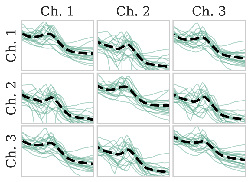
(a) Source cross-PSD

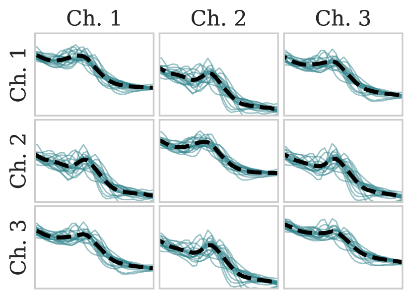
(b) Alignment with $f=32$

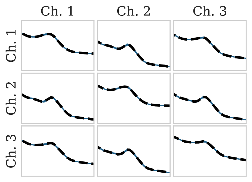
(c) Alignment with $f=256$

Figure 5: Illustration of the STMA method on sleep staging data. (a) The cross-PSD of the barycenter ($\boldsymbol{--}$) is computed from all the cross-PSD of the source domains. (b) The cross-PSDs of the source are aligned with the Monge mapping with a small filter size. (c) The cross-PSDs of the source are aligned with the Monge mapping with a big filter size. The bigger the filter size is, the more the cross-PSD are well aligned.

$f$-Monge maps computation (algorithm 1, line 3)

The third step consists of computing the $f$-Monge maps $m_{f,k}$ for all $k\in\left\llbracket 1,n_{d}\right\rrbracket\,$. The latter maps the $k^{\text{th}}$ source distribution to the barycenter. The formulas of $m_{f,k}$ are provided in Propositions 4, 7 and 10 for STMA, TMA and SMA respectively and only involves quantities computed in the first two steps, i.e., covariance matrices and barycenters. An illustration of the effect of applying the $f$-Monge maps is shown in 5(b) and 5(c) for different filter sizes.

Predictor training (algorithm 1, line 4)

The final step is to train a supervised predictor $h$, belonging to a function space $\Omega$, on the aligned source data. The trained model is

$$\widehat{h}\in\mathop{\rm arg\,min}_{h\in\Omega}\;\sum_{k=1}^{n_{d}}\mathcal{L}\left(\mathbf{y}_{k},h\left(\widehat{m}_{f,k}(\mathbf{X}_{k})\right)\right)$$ (22)

where $\mathbf{X}_{k}$ is the multivariate signal of the $k^{\text{th}}$ domain and $\mathcal{L}$ is a supervised loss function.

4.1.2 Test-time

At test-time, we have access to a new unlabeled target domain $\mathbf{X}_{t}\in\mathbb{R}^{n_{c}\times n_{\ell}}$. Notably, during this phase, the source domains are no longer accessible, and we rely solely on both the source barycenter $\widehat{\overline{\boldsymbol{\Sigma}}}$ and the trained predictor $\widehat{h}$, both computed at train time. The two first steps are the computations of the target covariance matrix and the $f$-Monge map $\widehat{m}_{f,t}$ from the target distribution to the barycenter (see lines 1 and 2 in algorithm 2). For the three methods, STMA, TMA, and SMA, the computations employ the same equations as in the train-time phase. Next, we predict the label using the trained predictor on the aligned target data (see line 3 in algorithm 2) with $\widehat{\mathbf{y}}_{t}=\widehat{h}\left(\widehat{m}_{f,t}(\mathbf{X}_{t})\right).$ It should be noted that the proposed test-time adaptation method requires only a small number of unlabeled samples from the target domain to estimate its covariance. Furthermore, the barycenter computation and predictor training occur during the training phase, eliminating the need for retraining during the test phase. Using MA, the trained predictor can still adapt to new temporal, spatial, or both shifts.

4.2 Computational aspects

We now discuss the computational aspects and numerial complexities of the proposed method STMA, TMA and SMA. The methods present interesting trade-offs between the costs of calculation and the shifts considered (spatial, temporal, or both). Indeed, the more shifts considered, the higher the calculation cost and conversely. This can motivate the practitioner to use one method rather than another, depending on the dimensions of the data and the observed shifts between domains. Then, the choice of the filter size $f$ is discussed.

4.2.1 Numerical complexity

Step	STMA	TMA	SMA
Covariance matrix computation	$\mathcal{O}\left(n_{d}n_{c}^{2}n_{\ell}f\log{f}\right)$	$\mathcal{O}\left(n_{d}n_{c}n_{\ell}f\log{f}\right)$	$\mathcal{O}\left(n_{d}n_{c}^{2}n_{\ell}\right)$
Barycenter computation	$\mathcal{O}\left(n_{d}n_{c}^{3}f\right)$ (per iter.)	$\mathcal{O}\left(n_{d}n_{c}f\right)$	$\mathcal{O}\left(n_{d}n_{c}^{3}\right)$ (per iter.)
Mapping computation	$\mathcal{O}\left(n_{d}(n_{c}^{3}f+n_{c}^{2}f\log f)\right)$	$\mathcal{O}\left(n_{d}n_{c}f\log f\right)$	$\mathcal{O}\left(n_{d}n_{c}^{3}\right)$
Mapping application	$\mathcal{O}\left(n_{d}n_{c}^{2}n_{\ell}f\right)$	$\mathcal{O}\left(n_{d}n_{c}n_{\ell}f\right)$	$\mathcal{O}\left(n_{d}n_{c}^{2}n_{\ell}\right)$

Table 2: Computational complexity comparison between STMA (spatio-temporal), TMA (temporal), and SMA (spatial). The complexity is expressed in terms of four key parameters: the number of domains $n_{d}$; the number of sensors $n_{c}$; the length of the signals $n_{\ell}$ and the filter size $f$.

The computational complexity of the four main operations at train and test times are studied below. The complexities are presented in Table 2 and depend on the number of sensors ($n_{c}$), signal length ($n_{\ell}$), and filter size ($f$), and vary depending on the method (STMA, SMA, or TMA). Note that all methods are linear in the number of domains and signal length. SMA does not consider temporal correlations, so its complexity is independent of the filter size $f$ (equivalent to $f=1$), contrary to STMA and TMA. In the same manner, TMA does not consider spatial correlations, so its complexity is linear in the number of sensors, contrary to STMA and SMA, which have cubic complexities. It should be noted that all operations are standard linear algebra and can be performed on modern hardware (CPU and GPU). A detailed explanation of the complexities is provided hereafter.

Covariance matrix computation

STMA and TMA use the Welch estimator with Fast Fourier Transform (FFT), which has a complexity of $\mathcal{O}(f\log f)$. TMA method has a linear complexity in the number of sensors, while the STMA and SMA methods are quadratic since they consider correlations between sensors.

Barycenter computation

This operation applies directly to the covariance matrices, making it independent of the signal length. TMA has a closed-form barycenter and linear complexity in the filter size and number of sensors, making it interesting for data with many sensors. STMA also has a complexity per iteration that is linear in the filter size. STMA and SMA have a cubic complexity in the sensor number because of the computations of Singular Value Decomposition (SVDs) to perform square roots and inverse square roots.

$f$-Monge maps computation

This operation also applies directly to the covariance matrices, making it independent of the signal length. In the worst case, the complexity per iteration of STMA is $f\log f$ (filter size). STMA and SMA have a cubic complexity in the sensor number because of the computations of SVDs. TMA has a linear complexity in the number of sensors, making it again appealing for data with many sensors.

$f$-Monge maps application

All the three methods are linear in the signal length. STMA and SMA involve a quadratic number of operations with respect to the number of sensors contrary to TMA which has a linear complexity.

4.2.2 Filter size selection

The proposed method introduces $f$, the filter size. This key hyper-parameter serves a dual role. Primarily, it contributes to reducing computation time; a benefit clearly demonstrated in Table 2 and subsubsection 4.2.1. Secondly, the filter size dictates the precision with which the PSDs of the domains are mapped to the barycenter. As visualized in Figure 4 and Figure 5, a larger filter size yields a more accurate mapping, while a smaller size only subtly adjusts the PSDs. This flexibility enables a balance between perfectly aligning the PSDs, which might compromise unique class features, and making sufficient adjustments to reduce noise and domain-specific variability while preserving class-specific characteristics.

4.3 Concentration bounds of the Monge Alignment

In this subsection, we propose concentration bounds for the estimations of STMA, TMA, and SMA mappings. These theorems provide a rigorous framework for understanding the reliability and precision of MA methods. Estimating OT plans is challenging due to the curse of dimensionality, with OT estimators generally decaying at a rate of $O(n^{-1/d})$, where $n$ is the number of observations and $d$ is the data dimension [46]. However, [40] propose a concentration bound for linear Monge mapping estimation with a faster convergence rate of $O(n^{-1/2})$, i.e., independent of the data dimension. This suggests greater accuracy and robustness in high-dimensional settings. Our proposed bounds account for two key aspects: mapping to the Wasserstein barycenter and using PSD computation with the Welch estimator. These bounds differ from [40], which maps to a given empirical covariance matrix. In particular, we leverage [47] to establish these bounds, highlighting an induced bias in PSD computation due to the Welch estimator. To introduce the concentration bound, we first define from [47] the spatial correlation of delay $\ell$, denoted $\mathbf{R}_{\ell}$, for signal following the Assumption 2, as

$$\mathbf{R}_{\ell}=\begin{pmatrix}({\boldsymbol{\Sigma}}_{1,1})_{1,\ell}&\dots&({\boldsymbol{\Sigma}}_{1,n_{c}})_{1,\ell}\\ \dots&\dots&\dots\\ ({\boldsymbol{\Sigma}}_{n_{c},1})_{1,\ell}&\dots&({\boldsymbol{\Sigma}}_{n_{c},n_{c}})_{1,\ell}\end{pmatrix}\in\mathcal{S}_{n_{c}}^{++}$$ (23)

For signals following Assumption 6 only the diagonal, $(r_{c})_{l}=({\boldsymbol{\Sigma}}_{c,c})_{1,\ell}$ is necessary.

4.3.1 STMA concentration bound

The next theorem introduces the general concentration bound, i.e., corresponding to STMA.

Theorem 12 (STMA concentration bound)

Let $\mathbf{X}_{t}\in\mathbb{R}^{n_{c}\times n_{\ell}}$ be a realization of $\operatorname{vec}(\mathbf{X})\sim\mathcal{N}(\mathbf{0},{\boldsymbol{\Sigma}}_{t})$. For $k\in\left\llbracket 1,K\right\rrbracket\,$, let $\mathbf{X}_{k}\in\mathbb{R}^{n_{c}\times n_{\ell}}$ be a realization of $\operatorname{vec}(\mathbf{X}_{k})\sim\mathcal{N}(\mathbf{0},{\boldsymbol{\Sigma}}_{k})$. Let us assume that ${\boldsymbol{\Sigma}}_{t}$ and ${\boldsymbol{\Sigma}}_{k}$ follow the Assumption 2, i.e., ${\boldsymbol{\Sigma}}_{t}=\mathbf{F}\mathbf{U}\mathbf{Q}_{t}\mathbf{U}^{\mkern-1.5mu\mathsf{T}}\mathbf{F}^{\mathsf{H}}$ and ${\boldsymbol{\Sigma}}_{k}=\mathbf{F}\mathbf{U}\mathbf{Q}_{k}\mathbf{U}^{\mkern-1.5mu\mathsf{T}}\mathbf{F}^{\mathsf{H}}$, that $\|\mathbf{R}_{\ell}\|_{2}\leq\gamma\rho^{|\ell|}$ with $\gamma>0$ and $\rho\in[0,1)$ and that only fixed point iteration of the barycenter is done. Then there exist numerical constants $c_{k}>0$, for all $k$, and $C>0$, independent from $n_{\ell}$, $n_{c}$, $n_{d}$ and $f$, such that with probability greater than $1-\delta$, we have

$$\|\widehat{\mathbf{A}}-\mathbf{A}\|\lesssim\left(C+\frac{1}{n_{d}}\sum_{k=1}^{n_{d}}c_{k}\right)\left(\mathchoice{\leavevmode\hbox to223.37pt{\vbox to23.08pt{\text{[drawing]}}}}{\leavevmode\hbox to223.37pt{\vbox to23.08pt{\text{[drawing]}}}}{\leavevmode\hbox to158.36pt{\vbox to16.16pt{\text{[drawing]}}}}{\leavevmode\hbox to115.02pt{\vbox to11.54pt{\text{[drawing]}}}}\right.\\ +\left.\mathchoice{\leavevmode\hbox to566.63pt{\vbox to31.36pt{\text{[drawing]}}}}{\leavevmode\hbox to566.63pt{\vbox to31.36pt{\text{[drawing]}}}}{\leavevmode\hbox to505.43pt{\vbox to13.51pt{\text{[drawing]}}}}{\leavevmode\hbox to378.8pt{\vbox to10.16pt{\text{[drawing]}}}}\right)\;, \mathstrut\delta 2\sum_{i=0}^{f-1}\frac{i}{n_{\ell}}\rho^{i}+\frac{2\delta\rho^{f}}{1-\rho} \mathstrut 2\widetilde{\mathbf{Q}}\max\left\{\frac{5}{2\frac{n_{\ell}}{f}}\log\left(5f^{2}\left(\frac{4\times 10^{2n_{c}}}{\delta}\right)^{32}\right),\sqrt{\frac{5}{2\frac{n_{\ell}}{f}}\log\left(5f^{2}\left(\frac{4\times 10^{2n_{c}}}{\delta}\right)^{32}\right)}\right\} \mathstrut\delta 2\sum_{i=0}^{f-1}\frac{i}{n_{\ell}}\rho^{i}+\frac{2\delta\rho^{f}}{1-\rho} \mathstrut 2\widetilde{\mathbf{Q}}\max\left\{\frac{5}{2\frac{n_{\ell}}{f}}\log\left(5f^{2}\left(\frac{4\times 10^{2n_{c}}}{\delta}\right)^{32}\right),\sqrt{\frac{5}{2\frac{n_{\ell}}{f}}\log\left(5f^{2}\left(\frac{4\times 10^{2n_{c}}}{\delta}\right)^{32}\right)}\right\}$$

with $\widetilde{\mathbf{Q}}=\max_{d\in\{1,\dots,n_{d},t\}}{\|\mathbf{Q}_{d}\|}_{\infty}$.

We made the choice to limit the theoretical analysis to only one iteration of the barycenter, allowing to provide this result. In practice, the barycenter converges fast, leading to good results after one iteration, and we did not observe performance gains with more iterations in our experiments. In contrast to the concentration bound proposed by [40], this bound includes a bias term resulting from the estimation of cross-PSDs using the Welch method. This bias depends on size of the filter $f$ the temporal correlation of the signal: higher correlation (large $\rho$) leads to greater bias, as shown on the left in Figure 6. However, the variance has a classical bound in $\mathcal{O}(\sqrt{f/n_{\ell}})$. Hence, the filter size can be adjusted to control the bias-variance trade-off. Figure 6 shows this trade-off with a dotted line, highlighting the optimal filter size.

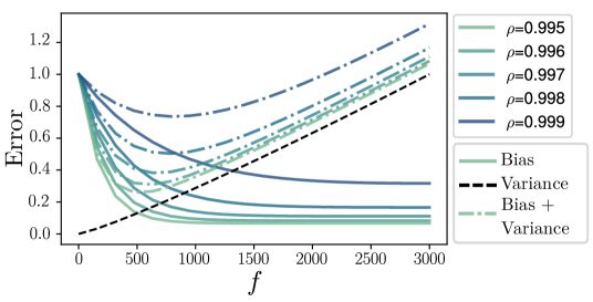
Figure 6: bias-variance estimation tradeoff versus the filter size $f$. For a given $\rho$, increasing the filter size reduces the bias, but at the cost of increased variance. A single optimal filter size range balances bias and variance, yielding a good tradeoff.

4.3.2 TMA concentration bound

TMA exhibits a similar concentration bound, i.e., with a bias-variance tradeoff and is exposed here-after.

Theorem 13 (TMA concentration bound)

Let $\mathbf{X}=[\mathbf{x}_{1},\dots,\mathbf{x}_{n_{c}}]^{\mkern-1.5mu\mathsf{T}}\in\mathbb{R}^{n_{c}\times n_{\ell}}$ be a realization of $\operatorname{vec}(\mathbf{X})\sim\mathcal{N}(\mathbf{0},{\boldsymbol{\Sigma}})$. For $k\in\left\llbracket 1,K\right\rrbracket\,$, let $\mathbf{X}_{k}\in\mathbb{R}^{n_{c}\times n_{\ell}}$ be a realization of $\operatorname{vec}(\mathbf{X}_{k})\sim\mathcal{N}(\mathbf{0},{\boldsymbol{\Sigma}}_{k})$. We assume that ${\boldsymbol{\Sigma}}$ and ${\boldsymbol{\Sigma}}_{k}$ follow Assumption 6, i.e., ${\boldsymbol{\Sigma}}=\mathbf{F}\operatorname{diag}(\mathbf{q}_{1},\dots,\mathbf{q}_{n_{c}})\mathbf{F}^{\mathsf{H}}$ and ${\boldsymbol{\Sigma}}_{k}=\mathbf{F}\operatorname{diag}(\mathbf{q}_{1}^{k},\dots,\mathbf{q}_{n_{c}}^{k})\mathbf{F}^{\mathsf{H}}$, and for every $c\in\left\llbracket 1,n_{c}\right\rrbracket\,$ $(r_{c})_{\ell}\leq\gamma\rho^{|\ell|}$ with $\delta>0$ and $\rho\in[0,1)$. For every $c\in\left\llbracket 1,n_{c}\right\rrbracket\,$, we denote by $\mathbf{p}_{c}=g_{f}(\mathbf{q}_{c})$, $\overline{\mathbf{p}}_{c}=g_{f}(\overline{\mathbf{q}}_{c})$, and $\mathbf{p}_{c,k}=g_{f}(\mathbf{q}_{c,k})$. Then there exists numerical constants $c_{c,k}^{\prime}>0$, for all $k$ and $C_{c}^{\prime}>0$ independent from $n_{\ell}$, $n_{c}$, $n_{d}$ and $f$, such that with probability greater than $1-\delta$, we have

$$\|\widehat{\mathbf{A}}-\mathbf{A}\|\lesssim\max_{c}\left(C^{\prime}_{c}+\sum_{k=1}^{n_{d}}c_{c,k}^{\prime}\right)\left(\mathchoice{\leavevmode\hbox to223.37pt{\vbox to23.08pt{\text{[drawing]}}}}{\leavevmode\hbox to223.37pt{\vbox to23.08pt{\text{[drawing]}}}}{\leavevmode\hbox to158.36pt{\vbox to16.16pt{\text{[drawing]}}}}{\leavevmode\hbox to115.02pt{\vbox to11.54pt{\text{[drawing]}}}}\right.\\ +\left.\mathchoice{\leavevmode\hbox to548.58pt{\vbox to31.36pt{\text{[drawing]}}}}{\leavevmode\hbox to548.58pt{\vbox to31.36pt{\text{[drawing]}}}}{\leavevmode\hbox to488.7pt{\vbox to13.51pt{\text{[drawing]}}}}{\leavevmode\hbox to366.85pt{\vbox to10.16pt{\text{[drawing]}}}}\right)\;. \mathstrut\delta 2\sum_{i=0}^{f-1}\frac{i}{n_{\ell}}\rho^{i}+\frac{2\delta\rho^{f}}{1-\rho} \mathstrut 2\widetilde{\mathbf{p}}_{c}\max\left\{\frac{5}{2\frac{n_{\ell}}{f}}\log\left(5f^{2}\left(\frac{4\times 10^{2}}{\delta}\right)^{32}\right),\sqrt{\frac{5}{2\frac{n_{\ell}}{f}}\log\left(5f^{2}\left(\frac{4\times 10^{2}}{\delta}\right)^{32}\right)}\right\} \mathstrut\delta 2\sum_{i=0}^{f-1}\frac{i}{n_{\ell}}\rho^{i}+\frac{2\delta\rho^{f}}{1-\rho} \mathstrut 2\widetilde{\mathbf{p}}_{c}\max\left\{\frac{5}{2\frac{n_{\ell}}{f}}\log\left(5f^{2}\left(\frac{4\times 10^{2}}{\delta}\right)^{32}\right),\sqrt{\frac{5}{2\frac{n_{\ell}}{f}}\log\left(5f^{2}\left(\frac{4\times 10^{2}}{\delta}\right)^{32}\right)}\right\}$$

with $\widetilde{\mathbf{p}}_{c}=\max_{d\in\{1,\dots,n_{d},t\}}{\|\mathbf{p}_{c,d}\|}_{\infty}$.

To the best of our knowledge, this is the first concentration bound of the method proposed by [34]. This bound includes bias and variance terms as in STMA concentration bound. The bound has similar behaviors but the independence of the channels leads to a smaller variance.

4.3.3 SMA concentration bound

Contrary to STMA and TMA, SMA has a concentration bound with a null bias. This makes it particularly suitable for short and highly correlated in time signals. Indeed, SMA ensures accurate estimations without the bias introduced by the temporal correlation.

Theorem 14 (SMA concentration bound)

Let $\mathbf{X}_{t}\in\mathbb{R}^{n_{c}\times n_{\ell}}$ be a realization of $\operatorname{vec}(\mathbf{X}_{t})\sim\mathcal{N}(\mathbf{0},{\boldsymbol{\Sigma}}_{t})$. For $k\in\left\llbracket 1,K\right\rrbracket\,$, let $\mathbf{X}_{k}\in\mathbb{R}^{n_{c}\times n_{\ell}}$ be a realization of $\operatorname{vec}(\mathbf{X}_{k})\sim\mathcal{N}(\mathbf{0},{\boldsymbol{\Sigma}}_{k})$. We assume that ${\boldsymbol{\Sigma}}_{t}$ and ${\boldsymbol{\Sigma}}_{k}$ follow Assumption 9, i.e., ${\boldsymbol{\Sigma}}_{t}=\mathbf{F}\mathbf{U}\mathbf{Q}_{t}\mathbf{U}^{\mkern-1.5mu\mathsf{T}}\mathbf{F}^{\mathsf{H}}$ and ${\boldsymbol{\Sigma}}_{k}=\mathbf{F}\mathbf{U}\mathbf{Q}_{k}\mathbf{U}^{\mkern-1.5mu\mathsf{T}}\mathbf{F}^{\mathsf{H}}$. Then there exist numerical constants $c_{k}>0$, for all $k$ and $C>0$ independent from $n_{\ell}$, $n_{c}$, $n_{d}$ and $f$, such that with probability greater than $1-\delta$, we have

$$\|\widehat{\mathbf{A}}-\mathbf{A}\|\lesssim\mathchoice{\leavevmode\hbox to517.47pt{\vbox to24.13pt{\text{[drawing]}}}}{\leavevmode\hbox to517.47pt{\vbox to24.13pt{\text{[drawing]}}}}{\leavevmode\hbox to366.22pt{\vbox to16.19pt{\text{[drawing]}}}}{\leavevmode\hbox to265.4pt{\vbox to11.56pt{\text{[drawing]}}}}\\ \mathchoice{\leavevmode\hbox to456.18pt{\vbox to16.25pt{\text{[drawing]}}}}{\leavevmode\hbox to456.18pt{\vbox to16.25pt{\text{[drawing]}}}}{\leavevmode\hbox to328.66pt{\vbox to11.38pt{\text{[drawing]}}}}{\leavevmode\hbox to243.64pt{\vbox to8.12pt{\text{[drawing]}}}}\;. \mathstrut\frac{1}{n_{d}}\sum_{k=1}^{n_{d}}c_{k}\|{\boldsymbol{\Sigma}}_{k}\|\max\left(\sqrt{\frac{\mathbf{r}({\boldsymbol{\Sigma}}_{k})}{n_{\ell}}},\frac{\mathbf{r}({\boldsymbol{\Sigma}}_{k})}{n_{\ell}},\sqrt{\frac{-\ln{\delta}}{n_{\ell}}},\frac{-\ln{\delta}}{n_{c}}\right) \mathstrut+C\|{\boldsymbol{\Sigma}}_{t}\|\max\left(\sqrt{\frac{\mathbf{r}({\boldsymbol{\Sigma}}_{t})}{n_{\ell}}},\frac{\mathbf{r}({\boldsymbol{\Sigma}}_{t})}{n_{\ell}},\sqrt{\frac{-\ln{\delta}}{n_{\ell}}},\frac{-\ln{\delta}}{n_{\ell}}\right) \mathstrut\frac{1}{n_{d}}\sum_{k=1}^{n_{d}}c_{k}\|{\boldsymbol{\Sigma}}_{k}\|\max\left(\sqrt{\frac{\mathbf{r}({\boldsymbol{\Sigma}}_{k})}{n_{\ell}}},\frac{\mathbf{r}({\boldsymbol{\Sigma}}_{k})}{n_{\ell}},\sqrt{\frac{-\ln{\delta}}{n_{\ell}}},\frac{-\ln{\delta}}{n_{c}}\right) \mathstrut+C\|{\boldsymbol{\Sigma}}_{t}\|\max\left(\sqrt{\frac{\mathbf{r}({\boldsymbol{\Sigma}}_{t})}{n_{\ell}}},\frac{\mathbf{r}({\boldsymbol{\Sigma}}_{t})}{n_{\ell}},\sqrt{\frac{-\ln{\delta}}{n_{\ell}}},\frac{-\ln{\delta}}{n_{\ell}}\right)$$

5 Experimental results

This section evaluates MA on different datasets. MA is first tested on two biosignals classification tasks. The first experiment extends results on sleep staging proposed in [34] by using multivariate signals (i.e., several channels) and thus exploiting the spatial information. The second experiment focuses on Brain-Computer Interface (BCI) Motor Imagery tasks, where spatial information is crucial to classify. Then, we extend our method to 2D signals (i.e., images) on a new custom MNIST dataset where each domain corresponds to a directional blur. We apply MA on this new dataset and show its efficiency to compensate for the blur.

5.1 Biosignal tasks

In this section, we investigate the impact of MA on two critical biosignal tasks: Sleep stage classification and Brain-Computer Interface (BCI). Each dataset is introduced alongside the alignment methodology proposed for these tasks.

5.1.1 Biosignal Datasets

Sleep Staging Datasets

We utilize four publicly available datasets: MASS [48], HomePAP [49], CHAT [50], and ABC [51], accessible via the National Sleep Research Resource [28]. Sleep staging is performed using 7-channel EEG signals across all datasets. The EEG channels considered are F3, F4, C3, C4, O1, O2, and A2, referenced to FPz. Each night’s data is segmented into 30-second samples with a sampling frequency of $f_{s}=100$ Hz.

Brain-Computer Interface Datasets

We employ five publicly available datasets: BCI Competition IV [52], Weibo2014 [53], PhysionetMI [54], Cho2017 [55], and Schirrmeister2017 [56], accessible through MOABB [57]. These datasets consists of two classes motor imagery tasks involving right-hand and left-hand movements. We utilize a common set of 22 channels across the datasets. The length of time series varies across datasets, and following [33], we extract a uniform segment of 3 seconds from the middle of each trial for improved consistency with a sampling frequency of $f_{s}=128$ Hz.

5.1.2 Spatial correlation alignment

The selected datasets have been extensively studied in recent years [35, 58, 29]. In particular, several studies have highlighted the critical need to address the domain shifts in biosignal data [33, 59, 32]. To compensate for these shifts, they proposed Riemannian Alignment (RA), which is a test-time DA method tailored for spatial shifts. For a multivariate signal $\mathbf{X}_{d}\in\mathbb{R}^{n_{c}\times n_{\ell}}$ from the domain $d$, this alignment is given by the following operation:

$$m_{\text{RA}}(X_{d})=\mathbf{M}_{d}^{-\frac{1}{2}}\mathbf{X}_{d}\;,$$ (24)

where $\mathbf{M}_{d}\in\mathcal{S}_{n_{c}}^{++}$ is the Riemannian mean of the covariance matrices of all samples from the domain $d$. In the following experiments, we compare RA with MA for sleep staging and BCI motor imagery.

5.1.3 Deep learning architectures and experimental setup

In our experiments, we used two different architectures and setups for sleep staging and BCI. For sleep staging, we referred to the approach described in [35], and for BCI, we followed the setup proposed by [56] as implemented in MOABB [57]. In the upcoming section, we provide a detailed description of these two setups.

Architecture

Many neural network architectures dedicated to sleep staging have been proposed [60, 58, 59, 61]. In the following, we choose to focus on the architecture proposed by [35] that is an end-to-end neural network proposed to deal with multivariate time series and is composed of two convolutional layers with non-linear activation functions.

For BCI, different neural network architectures have been developed specifically [56, 62]. We focus on ShallowFBCSPNet [56], which is an end-to-end neural network proposed to deal with multivariate time series based on convolutional layers and filter bank common spatial patterns (FBCSP). Both architectures are implemented in braindecode package [56].

Training setup

The training parameters follows the reference implementations of [35] and [56] detailed below for reproducibility. For sleep staging experiment, we use the Adam optimizer with a learning rate of $10^{-3}$, $\beta_{1}=0.9$, and $\beta_{2}=0.999$. The batch size is set to $128$, and the early stopping is done on a validation set corresponding to $20\%$ of the subjects in the training set with a patience of $15$ epochs. We optimize the cross-entropy with class weight for all methods, which amounts to optimizing for balanced accuracy (BACC). Each experiment is done ten times with a different seed.

For BCI, we use the Adam optimizer with a cosine annealing learning rate scheduler starting at $6.25\times 10^{-4}$. The batch size is set to $128$, and the training is stopped after 200 epochs. No validation set is used. We optimize the cross-entropy for all methods. We report the average accuracy score (ACC) across ten different seeds.

Filter size and Welch’s parameters

MA requires tuning the filter size $f$ parameters. Yet, experiments show that this parameter is not critical, as good performances are observed over a large range of values. We provide a sensitivity analysis of the performance for different parameters in Figure 7 for sleep staging (left) and BCI (right). It shows that the value $f=256$ is a good trade-off for the sleep application while a value of $f=8$ is better for BCI. These parameter values are used in what follows. For the Welch method, we use a Hann window [63] and an overlap of $\frac{f}{2}$.

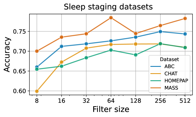
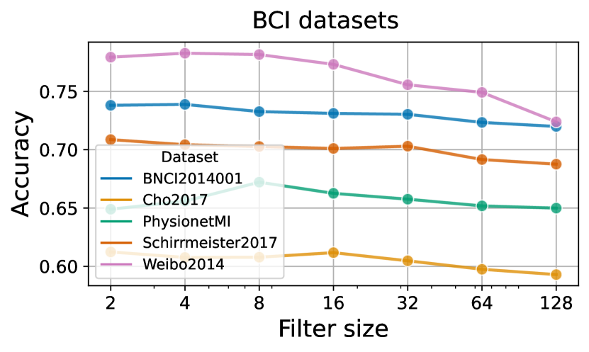
Figure 7: Evolution of the balanced accuracy score for a leave-one-dataset-out experiment for different values of filter size $f$.

5.2 Application to sleep staging

In our investigation, we build on the findings of [34] who showed the benefits of TMA for sleep staging when using only two sensors. Here, we incorporate more spatial information by using 7 EEG channels, as detailed in Section 5.1.1. This multidimensional dataset offers a more comprehensive perspective, thereby demonstrating the utility of STMA and SMA. In what follows, one subject is considered as one domain.

5.2.1 Comparison between different alignments

Historically, sleep staging has relied on neural networks processing raw data [60]. [35] improved this by applying z-score normalization to 30-second windows, removing local trends. More recently, [36] introduced session-wide normalization to eliminate global trends. Among these, window-based normalization, denoted as “No Align”, has proven most effective in [34] and will be used as baseline in the following. In our work, we also compare MA with RA to evaluate performance comprehensively.

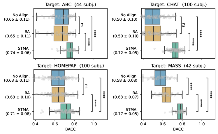
Figure 8: Balanced accuracy for sleep stage classification without alignment (blue), with RA (yellow), and with STMA (green) for different datasets in the target domain. Each dot represents one subject. STMA outperforms alternative methods for each target dataset. The number of stars illustrates the level of significance with a Wilcoxon test (ns: non-significative, $**$: $10^{-2}$, $***$: $10^{-3}$, or $****$: $10^{-4}$).

Using a leave-one-dataset-out evaluation (4-fold across dataset adaptation), results in Figure 8 show that standard z-score normalization struggles with dataset adaptation, with accuracies below 66%, sometimes dropping below 50% (e.g., CHAT dataset). Spatio-temporal alignment improves accuracy, with STMA consistently above 70% and even reaching an improvement of 2̃0% for MASS and CHAT. On the other hand, RA stagnates for three datasets (i.e., ABC, CHAT and HOMEPAP) and increase the score for only MASS by 5%. This underscores the importance of temporal information in sleep classification, beyond RA’s spatial focus. The experiment highlights the benefits of spatiotemporal alignment: higher accuracy and lower variance, suggesting that underperforming subjects improve the most. The next section will explore these subjects further.

5.2.2 Study of performance on low-performing domains

In this section, we evaluate the performance of individuals to identify the subjects that benefit from the most significant improvements. In the Figure 9, we propose to compare the accuracy without alignment ($x$-axis) and with spatio-temporal alignment ($y$-axis). A subject (i.e., a dot) above the line $y=x$ means that the alignment increases its score. For each adaptation, more than 85% of the dots are above the line, indicating a systematic increase in alignment for each domain. This number is even close to 100% for CHAT and MASS datasets. The rate of increase can vary for each subject. We color the dots by the $\Delta$BACC, representing the difference between the balanced accuracy with and without alignment. The darker the dots are, the better the $\Delta$BACC is. On the scatter plot, the more low-performing subjects (i.e., dots on the left) increase more than the other subjects.

To highlight our findings, we propose the Table 3 that reports the mean and variance of the $\Delta$BACC. Furthermore, we also report the $\Delta$BACC@20 metric, proposed in [34], which is the variation of balanced accuracy for the 20% lowest-performing subjects (i.e., the subjects with the lowest scores without alignment). For each adaptation, the gain is almost double for the low-performing subjects compared to all subjects. Hence, STMA is valuable for medical applications where a low failure rate is more important than a high average accuracy.

Target	$\Delta$BACC@20	$\Delta$BACC
ABC	0.21 $\pm$ 0.06	0.08 $\pm$ 0.08
CHAT	0.33 $\pm$ 0.07	0.21 $\pm$ 0.10
HOMEPAP	0.17 $\pm$ 0.11	0.09 $\pm$ 0.08
MASS	0.27 $\pm$ 0.07	0.20 $\pm$ 0.07

Table 3: Difference of BACC with STMA and without alignment in sleep staging for all the subjects ($\Delta$BACC column) and the 20% lowest-performing subjects ($\Delta$BACC@20 column).

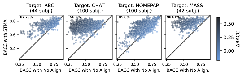
Figure 9: Balanced accuracy for sleep staging with STMA and without alignment. Each dot represents a subject. The size of the difference between the scores is directly proportional to the darkness of the dot. Darker dots are located on the left (i.e., lower-performing subjects). The percentage of the dots above and below the black diagonal line is given on the bottom left.

5.2.3 Impact of spatial and temporal information

The previous experiment shows the benefit of alignment for sleep staging, especially when spatio-temporal information is used. In this section we propose to apply a SMA (i.e., no temporal correlation) or TMA (i.e., no spatial correlation) on the sleep data. The Figure 10 shows the results of these methods for a leave-one-dataset-out experiment compared to without alignment and with spatio-temporal alignment.

As intended, the pure spatial alignment struggles to improve the accuracy for each adaptation except for MASS, while pure temporal alignment improves the BACC by 10% on average. It can be explained by the fact that the frequency-specific activity of the brain is critical for sleep classification. In contrast, spatial activity only brings marginal gains mainly due to channel redundancy except for MASS where RA and SMA succeed to increase slightly the score. However, the spatio-temporal alignment is statistically better than both single alignments. STMA combines both alignments, providing the best of both worlds.

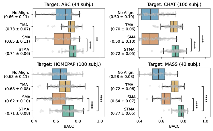
Figure 10: BACC for sleep stage classification with the different MAs. The number of stars illustrates the level of statistical significance (ns: non-significant, $**$: $10^{-2}$, or $****$: $10^{-4}$).

5.3 Application to Brain Computer Interface (BCI)

In sleep staging experiments, it has been demonstrated that spatio-temporal alignment is beneficial. Temporal information is essential for such a classification task. In this section, we aim to evaluate the effectiveness of this alignment technique on another biosignal task. While BCI relies less on temporal information for motor imagery classification, spatial information is crucial for distinguishing between classes.

5.3.1 Comparison between different alignments

If Riemannian alignment was a new approach in sleep staging, it is often used in BCI applications [33, 29, 59]. In previous studies, adaptation was done within one dataset or between two datasets. We propose a new BCI leave-one-dataset-out experiment setup that compares results using 5 folds across datasets adaptation.

Table 4 compares scores between no alignment, RA, and STMA in leave-one-dataset-out settings. Alignments improve scores for each dataset. However, both methods exhibits similar performances. For three datasets, the two methods perform the same, when for the BNCI2014001 dataset STMA outperforms RA by 2% and RA outperforms by 2% STMA for Cho2017 dataset. The BCI datasets have a low number of subjects, making a Wilcoxon test unreliable within each dataset. To address this issue and increase statistical power, we perform a Wilcoxon test by pooling together all subjects from the five datasets. The Figure 11 shows the comparison of the accuracy with STMA and without alignment (on the left) and with RA (on the right). The Wilcoxon test reveals that the first comparison exhibits a significant difference (p-value = $10^{-4}$) when 62% of the subjects were increased. The second comparison between STMA and RA showed a moderate difference in favor of RA, as indicated by the p-value.

Motor Imagery BCI classification relies primarily on spatial information compared to sleep staging, making the RA well-suited for the task; however, STMA still contributes to increasing the score, and it works even better in one scenario.

Dataset Target	BNCI2014001	Cho2017	PhysionetMI	Schirrmeister2017	Weibo2014
No Align.	0.70 $\pm$ 0.15	0.61 $\pm$ 0.09	0.63 $\pm$ 0.14	0.62 $\pm$ 0.14	0.70 $\pm$ 0.15
RA	0.72 $\pm$ 0.14	0.63 $\pm$ 0.09	0.66 $\pm$ 0.15	0.71 $\pm$ 0.14	0.77 $\pm$ 0.14
STMA	0.74 $\pm$ 0.12	0.61 $\pm$ 0.08	0.66 $\pm$ 0.12	0.71 $\pm$ 0.12	0.77 $\pm$ 0.14

Table 4: Accuracy score for BCI Motor Imagery for 5 different datasets as target. Both RA and STMA methods improve the score. STMA is the best in three out of five scenarios.

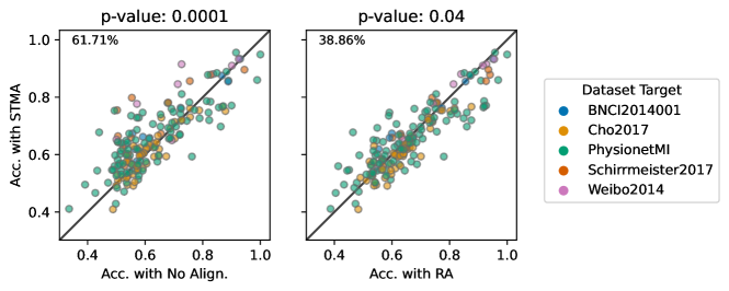
Figure 11: Comparison of the accuracy in BCI with STMA against No Align. and RA for each subject in target (colorized by dataset). The p-values are given at the top of the plot. The percentage of the dots above and below the black diagonal line is given on the bottom left.

5.3.2 Impact of spatial and temporal informations

The previous section suggests that the spatial information is the most valuable part of spatio-temporal filtering. We propose comparing pure spatial and temporal alignment with STMA in this section to support this statement. The Table 5 shows the results for 5-fold leave-one-dataset-out for all the MAs. After aligning the data, spatio-temporal is the best option except for Cho2017, where no alignment works. However, when the temporal alignment improves slightly, spatial alignment achieves almost the same accuracy as STMA on average.

Due to the specificities of the data, the BCI experiment leads to different conclusions than sleep staging about the impact of spatial and temporal filtering. Choosing the appropriate filtering method (spatial or temporal) based on the data allows for a quick and efficient alignment.

Dataset Target	BNCI2014001	Cho2017	PhysionetMI	Schirrmeister2017	Weibo2014
No Align.	0.70 $\pm$ 0.15	0.61 $\pm$ 0.09	0.63 $\pm$ 0.14	0.62 $\pm$ 0.14	0.70 $\pm$ 0.15
TMA	0.71 $\pm$ 0.12	0.58 $\pm$ 0.07	0.63 $\pm$ 0.12	0.69 $\pm$ 0.12	0.73 $\pm$ 0.12
SMA	0.74 $\pm$ 0.12	0.61 $\pm$ 0.08	0.65 $\pm$ 0.13	0.71 $\pm$ 0.12	0.77 $\pm$ 0.13
STMA	0.74 $\pm$ 0.12	0.61 $\pm$ 0.08	0.66 $\pm$ 0.12	0.71 $\pm$ 0.12	0.77 $\pm$ 0.14

Table 5: Study of the impact of spatial and temporal informations on accuracy score for BCI Motor Imagery for 5 different datasets as target. STMA is almost always the best one, but SMA also provides a good alignment.

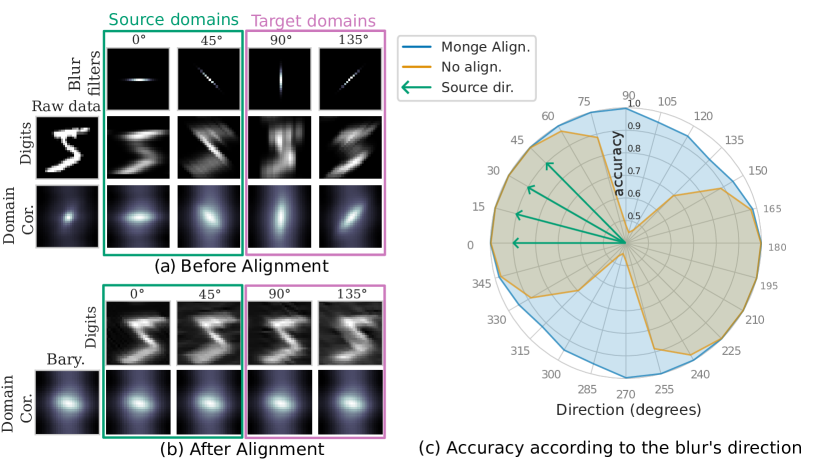
Figure 12: Blur MNIST visualization. The figure shows the sample and correlation for four blurred domains in different directions (a) before alignment and (b) after MA. (c) Accuracy of classification when trained on data containing only four blur directions (0°, 15°, 30°, and 45°) and testing on all possible directions. The accuracy drops when the testing data are blurred differently from the train. With MA, the accuracy improves significantly and is uniformly above 0.9.

5.4 Illustration of MA on 2D signals

The previous experiments demonstrate the efficiency of MA on multivariate time series. Here, we want to illustrate the potential impact of the proposed methods beyond time series by considering images (i.e., 2D signals). On those signals, convolution and FFT are extended to 2D, allowing us to adapt MA with 2D filters. To illustrate the effect of 2D MA, we introduce a new custom multi-directional blur MNIST dataset.

Toy dataset

One considers a the toy dataset created from the digits classification dataset MNIST [64]. This dataset consists of several domains where the digits are blurred in one direction. In the Figure 12, in the top left, four different domains are plotted with respective blur directions (i.e., 0°, 45°, 90°, and 135°). The effect of the blur is clearly visible on both the raw digits and the correlation of the domains. For analysis, twelve domains are created with a blurred direction ranging from 0° to 165°. Note that the blur is symmetric, which means that the blur directions from 180° to 345° are also covered.

Training setup

The goal is to train on a subset of domains and predict the left-out domains. The source domains are the ones with directions going from 0° to 45° (i.e., the green arrows on the right of Figure 12). The target domains are the remaining ones (60° to 165°). To train the classifier, we use the architecture in the MNIST example of PyTorch. We use a Convolutional Neural Network (CNN) as a classifier. We use a batch size of 1000 and a learning rate of 1 with the Adadelta optimizer from PyTorch [65]. We stop the training when the validation loss does not decrease after ten epochs.

2D MA on blurred MNIST

In this problem, the images are considered like 2D signals. One can compute an estimation of the PSD of an image with the squared FFT. The PSD of a domain is then the average of the PSD of all images of the given domain. Taking the inverse Fourier of the PSD of one domain provides the domain correlation. To align the domain, first, the PSD barycenter is computed on the PSD of the source domains (i.e., 0° to 45°). The resulting correlation of the barycenter is given in the left of Figure 12 (b). Since the source domains are concentrated in a specific range of directions, the correlation of the barycenter is focused on these directions. After computing the barycenter, one can apply the Monge mapping with 7 since we have univariate 2D signals here. The digits and the correlation after alignment are given in Figure 12 (b). Now, the correlation of all the domains, source, or target is the same, and the digits look more alike.

Results with and without alignment

One classifier is trained on domains that are not aligned, and another classifier is trained on aligned domains. The results are plotted on a spider plot in Figure 12 (c). The angle corresponds to the blur directions of the domain. The radius corresponds to the accuracy of the predictions. For no alignment (orange line), the accuracy is close to 1 for blur direction from 0° to 45°, which is logical since it is the data used for training. However, as soon as the domains get further from the train angles, the accuracy decreases to reach the lowest score of 0.55 for the angle 105°. After using MA, the accuracy still decreased after getting away from 0° and 45° but stays above 0.9 of the accuracy score. Aligning the models helps classify unseen domains, even if the blur directions differ. This simulated example shows that the method MA is generic and can be extended to multi-dimensional signals.

6 Conclusions

In this paper, we proposed Spatio-Temporal Monge Alignment (STMA), an Optimal Transport (OT) based method for multi-source and test-time Domain Adaptation (DA) of multivariate signals. Our approach addresses the variability present in signals due to different recording conditions or hardware devices, which often leads to performance drops in machine learning applications. STMA aligns signals’ cross-power spectrum density (cross-PSD) to the Wasserstein barycenter of source domains, enabling predictions for new domains without retraining. We also introduced two special cases of the method: Temporal Monge Alignment (TMA) and Spatial Monge Alignment (SMA), each tailored for specific shift assumptions. Our theoretical analysis provided non-asymptotic concentration bounds for the mapping estimation, demonstrating a bias-plus-variance error structure with a favorable variance decay rate of $\mathcal{O}(n_{\ell}^{-1/2})$. Our numerical experiments on images and multivariate biosignal data, specifically in sleep staging and Brain-Computer Interface (BCI) tasks, showed that STMA leads to significant and consistent performance improvements over state-of-the-art methods. Importantly, STMA serves as a pre-processing step and is compatible with both shallow and deep learning methods, enhancing their performance without requiring refitting or access to source data at test-time. In summary, STMA provides an efficient, solution to domain adaptation challenges in multivariate signal processing. Since it remains simple and requires only covariance estimation, it can be adapted to privacy preserving applications using differential private covariances [66] .

7 Supplementary Materials

7.1 Proof of Proposition 1: PSD and filter sub-sampling

Given $t\in\left\llbracket 1,f\right\rrbracket\,$, and since $(\mathbf{A})_{1l}=0$ for $l\not\in\mathfrak{I}\triangleq\left\llbracket 1,\left\lceil{f/2}\right\rceil\right\rrbracket\,\cup\llbracket n_{\ell}-\left\lfloor{f/2}\right\rfloor+1,n_{\ell}\rrbracket$, we have

$$\left(\frac{1}{\sqrt{f}}\mathbf{F}_{f}^{\mathsf{H}}\mathbf{p}\right)_{t} =\frac{1}{f}\sum_{l=1}^{f}\exp\left(2i\pi\frac{(l-1)(t-1)}{f}\right)(\mathbf{p})_{l}$$

$$=\frac{1}{f}\sum_{l=1}^{f}\exp\left(2i\pi\frac{(l-1)(t-1)}{n_{\ell}}\frac{n_{\ell}}{f}\right)(\mathbf{q})_{\frac{(l-1)n_{\ell}}{f}+1}$$

$$=\frac{1}{f}\sum_{\begin{subarray}{c}m\in\{1,\frac{n_{\ell}}{f}+1,\dots,\\ \frac{(f-1)n_{\ell}}{f}+1\}\end{subarray}}\exp\left(2i\pi\frac{(m-1)(t-1)}{n_{\ell}}\right)(\mathbf{q})_{m}$$

$$=\frac{1}{f}\sum_{\begin{subarray}{c}m\in\{1,\frac{n_{\ell}}{f}+1,\dots,\\ \frac{(f-1)n_{\ell}}{f}+1\}\end{subarray}}\sum_{l=1}^{n_{\ell}}\exp\left(-2i\pi\frac{(m-1)(l-t)}{n_{\ell}}\right)(\mathbf{A})_{1l}$$

$$=\frac{1}{f}\sum_{l=1}^{n_{\ell}}\sum_{k=0}^{f-1}\exp\left(-2i\pi\frac{k(l-t)}{f}\right)(\mathbf{A})_{1l}$$

$$=\frac{1}{f}\sum_{l\in\mathfrak{I}}\sum_{k=0}^{f-1}\exp\left(-2i\pi\frac{k(l-t)}{f}\right)(\mathbf{A})_{1l}\enspace.$$

Then, we split the sum over $l$ with terms such that $l-t$ is a multiple of $f$, denoted $l-t\propto f$, and terms where $l-t$ is not a multiple of $f$, denoted $l-t\not\propto f$,

$$\left(\frac{1}{\sqrt{f}}\mathbf{F}_{f}^{\mathsf{H}}\mathbf{p}\right)_{t} =\frac{1}{f}\sum_{\begin{subarray}{c}l\in\mathfrak{I}\\ l-t\propto f\end{subarray}}\sum_{k=0}^{f-1}\underbrace{\exp\left(-2i\pi\frac{k(l-t)}{f}\right)}_{=1}(\mathbf{A})_{1l}+\frac{1}{f}\sum_{\begin{subarray}{c}l\in\mathfrak{I}\\ l-t\not\propto f\end{subarray}}\sum_{k=0}^{f-1}\exp\left(-2i\pi\frac{k(l-t)}{f}\right)(\mathbf{A})_{1l}$$

$$=\sum_{\begin{subarray}{c}l\in\mathfrak{I}\\ l-t\propto f\end{subarray}}(\mathbf{A})_{1l}+\frac{1}{f}\sum_{\begin{subarray}{c}l\in\mathfrak{I}\\ l-t\not\propto f\end{subarray}}\underbrace{\frac{1-\exp\left(-2i\pi(l-t)\right)}{1-\exp\left(-2i\pi\frac{(l-t)}{f}\right)}}_{=0}(\mathbf{A})_{1l}=\sum_{\begin{subarray}{c}l\in\mathfrak{I}\\ l-t\propto f\end{subarray}}(\mathbf{A})_{1l}\enspace.$$

Case $t\in\left\llbracket 1,\left\lceil{f/2}\right\rceil\right\rrbracket\,$:

Given $t\in\left\llbracket 1,\left\lceil{f/2}\right\rceil\right\rrbracket\,$ and $l\in\mathfrak{I}$. Since $n_{\ell}\propto f$, there exists $k\in\mathbb{Z}$ such that $l-t\in\llbracket 1-\left\lceil{f/2}\right\rceil,\left\lceil{f/2}\right\rceil-1\rrbracket\cup\llbracket(k-1)f+1,kf-1\rrbracket$. Since $l-t\propto f$, we get that $l-t=0$ and thus,

$$\left(\frac{1}{\sqrt{f}}\mathbf{F}_{f}^{\mathsf{H}}\mathbf{p}\right)_{t}=(\mathbf{A})_{1t}\enspace.$$

Case $t\in\llbracket\left\lceil{f/2}\right\rceil+1,f\rrbracket$:

Given $t\in\llbracket\left\lceil{f/2}\right\rceil+1,f\rrbracket$ and $l\in\mathfrak{I}$, we get that $l-t\in\llbracket-f+1,-1\rrbracket\cup\llbracket n_{\ell}-\left\lfloor{f/2}\right\rfloor-f+1,n_{\ell}-\left\lfloor{f/2}\right\rfloor-1\rrbracket$. Since $n_{\ell}\propto f$ and $l-t\propto f$, it implies that $l-t=n_{\ell}-f$. Hence, we get that

$$\left(\frac{1}{\sqrt{f}}\mathbf{F}_{f}^{\mathsf{H}}\mathbf{p}\right)_{t}=(\mathbf{A})_{1(n_{\ell}-f+t)}\enspace.$$

7.2 Proof of Proposition 4: spatio-temporal mapping

We recall that the Monge mapping is

$$\mathbf{A}={\boldsymbol{\Sigma}}_{s}^{-\frac{1}{2}}\left({\boldsymbol{\Sigma}}_{s}^{\frac{1}{2}}{\boldsymbol{\Sigma}}_{t}{\boldsymbol{\Sigma}}_{s}^{\frac{1}{2}}\right)^{\frac{1}{2}}{\boldsymbol{\Sigma}}_{s}^{-\frac{1}{2}}\;.$$

We inject the decomposition from the Equation 15, i.e., ${\boldsymbol{\Sigma}}_{d}=\mathbf{F}\mathbf{U}\mathbf{Q}_{d}\mathbf{U}^{\mkern-1.5mu\mathsf{T}}\mathbf{F}^{\mathsf{H}}$ for $d\in\{s,t\}$ in the Monge mapping. Since $\mathbf{F}\mathbf{U}$ is an unitary matrix, for every $\mathbf{Q}\in{\mathcal{H}_{n_{c}n_{\ell}}^{++}}$, we have $(\mathbf{F}\mathbf{U}\mathbf{Q}\mathbf{U}^{\mkern-1.5mu\mathsf{T}}\mathbf{F}^{\mathsf{H}})^{-\frac{1}{2}}=\mathbf{F}\mathbf{U}{\mathbf{Q}}^{-\frac{1}{2}}\mathbf{U}^{\mkern-1.5mu\mathsf{T}}\mathbf{F}^{\mathsf{H}}$. Hence, we get

$$\mathbf{A} =\mathbf{F}\mathbf{U}\mathbf{Q}_{s}^{-\frac{1}{2}}\mathbf{U}^{\mkern-1.5mu\mathsf{T}}\mathbf{F}^{\mathsf{H}}\left(\mathbf{F}\mathbf{U}\mathbf{Q}_{s}^{\frac{1}{2}}\mathbf{U}^{\mkern-1.5mu\mathsf{T}}\mathbf{F}^{\mathsf{H}}\mathbf{F}\mathbf{U}\mathbf{Q}_{t}\mathbf{U}^{\mkern-1.5mu\mathsf{T}}\mathbf{F}^{\mathsf{H}}\mathbf{F}\mathbf{U}\mathbf{Q}_{s}^{\frac{1}{2}}\mathbf{U}^{\mkern-1.5mu\mathsf{T}}\mathbf{F}^{\mathsf{H}}\right)^{\frac{1}{2}}\mathbf{F}\mathbf{U}\mathbf{Q}_{s}^{-\frac{1}{2}}\mathbf{U}^{\mkern-1.5mu\mathsf{T}}\mathbf{F}^{\mathsf{H}}$$

$$=\mathbf{F}\mathbf{U}\mathbf{Q}_{s}^{-\frac{1}{2}}\mathbf{U}^{\mkern-1.5mu\mathsf{T}}\mathbf{F}^{\mathsf{H}}\mathbf{F}\mathbf{U}\left(\mathbf{Q}_{s}^{\frac{1}{2}}\mathbf{Q}_{t}\mathbf{Q}_{s}^{\frac{1}{2}}\right)^{\frac{1}{2}}\mathbf{U}^{\mkern-1.5mu\mathsf{T}}\mathbf{F}^{\mathsf{H}}\mathbf{F}\mathbf{U}\mathbf{Q}_{s}^{-\frac{1}{2}}\mathbf{U}^{\mkern-1.5mu\mathsf{T}}\mathbf{F}^{\mathsf{H}}=\mathbf{F}\mathbf{U}\mathbf{Q}_{s}^{-\frac{1}{2}}\left(\mathbf{Q}_{s}^{\frac{1}{2}}\mathbf{Q}_{t}\mathbf{Q}_{s}^{\frac{1}{2}}\right)^{\frac{1}{2}}\mathbf{Q}_{s}^{-\frac{1}{2}}\mathbf{U}^{\mkern-1.5mu\mathsf{T}}\mathbf{F}^{\mathsf{H}}\;.$$

Furthermore, $\mathbf{Q}_{s}^{-\frac{1}{2}}\left(\mathbf{Q}_{s}^{\frac{1}{2}}\mathbf{Q}_{t}\mathbf{Q}_{s}^{\frac{1}{2}}\right)^{\frac{1}{2}}\mathbf{Q}_{s}^{-\frac{1}{2}}$ is a block-diagonal matrix since $\mathbf{Q}_{s}$ and $\mathbf{Q}_{t}$ are block-diagonal matrices. Thus, there exists $\mathbf{q}_{i,j}\in{\mathbb{C}^{n_{\ell}}}$ for $i,j\in\left\llbracket 1,n_{c}\right\rrbracket\,$ such that

$$\mathbf{A}=\mathbf{F}\begin{pmatrix}\operatorname{diag}(\mathbf{q}_{1,1})&\dots&\operatorname{diag}(\mathbf{q}_{1,n_{c}})\\ \dots&\dots&\dots\\ \operatorname{diag}(\mathbf{q}_{n_{c},1})&\dots&\operatorname{diag}(\mathbf{q}_{n_{c},n_{c}})\end{pmatrix}\mathbf{F}^{\mathsf{H}}\;.$$

It follows that the block matrices of $\mathbf{A}$ are $\mathbf{A}_{i,j}=\mathbf{F}_{n_{\ell}}\operatorname{diag}(\mathbf{q}_{i,j})\mathbf{F}_{n_{\ell}}^{\mathsf{H}}$ for $i,j\in\left\llbracket 1,n_{c}\right\rrbracket\,$. Then, the $f$-Monge mapping $\widetilde{\mathbf{A}}$ introduced in the Definition 3 has block matrices $\widetilde{\mathbf{A}}_{i,j}=\mathcal{P}_{f}(\mathbf{A}_{i,j})$ for $i,j\in\left\llbracket 1,n_{c}\right\rrbracket\,$. Hence, given $\mathbf{X}=[\mathbf{x}_{1},\dots,\mathbf{x}_{n_{c}}]^{\mkern-1.5mu\mathsf{T}}\in\mathbb{R}^{n_{c}\times n_{\ell}}$, the $f$-Monge mapping is

$$m_{f}\left(\mathbf{X}\right) =\operatorname{vec}^{-1}\left(\widetilde{\mathbf{A}}\operatorname{vec}(\mathbf{X})\right)$$

$$=\operatorname{vec}^{-1}\left(\begin{pmatrix}\mathcal{P}_{f}(\mathbf{A}_{1,1})&\dots&\mathcal{P}_{f}(\mathbf{A}_{1,C})\\ \dots&\dots&\dots\\ \mathcal{P}_{f}(\mathbf{A}_{C,1})&\dots&\mathcal{P}_{f}(\mathbf{A}_{C,C})\end{pmatrix}\begin{pmatrix}\mathbf{x}_{1}\\ \vdots\\ \mathbf{x}_{n_{c}}\end{pmatrix}\right)=\operatorname{vec}^{-1}\begin{pmatrix}\sum_{j=1}^{n_{c}}\mathcal{P}_{f}(\mathbf{A}_{1,j})\mathbf{x}_{j}\\ \vdots\\ \sum_{j=1}^{n_{c}}\mathcal{P}_{f}(\mathbf{A}_{C,j})\mathbf{x}_{j}\end{pmatrix}\;.$$

Hence, from Proposition 1, we get

$$m_{f}\left(\mathbf{X}\right)=\left[\sum_{j=1}^{n_{c}}\mathbf{h}_{1,j}*\mathbf{x}_{j},\dots,\sum_{j=1}^{n_{c}}\mathbf{h}_{C,j}*\mathbf{x}_{j}\right]^{\mkern-1.5mu\mathsf{T}}$$

where $\mathbf{h}_{i,j}=\frac{1}{\sqrt{f}}\mathbf{F}_{f}^{\mathsf{H}}\mathbf{p}_{i,j}$ and $\mathbf{p}_{i,j}=g_{f}(\operatorname{diag}(\mathbf{F}_{n_{\ell}}^{\mathsf{H}}\mathcal{P}_{f}(\mathbf{A}_{i,j})\mathbf{F}_{n_{\ell}}))=g_{f}(\mathbf{q}_{i,j})$. Denoting

$$\mathbf{Q}\triangleq\operatorname{diag}\left(\mathbf{B}_{1},\dots,\mathbf{B}_{n_{\ell}}\right)\triangleq\mathbf{Q}_{s}^{-\frac{1}{2}}\left(\mathbf{Q}_{s}^{\frac{1}{2}}\mathbf{Q}_{t}\mathbf{Q}_{s}^{\frac{1}{2}}\right)^{\frac{1}{2}}\mathbf{Q}_{s}^{-\frac{1}{2}}\in\mathbb{R}^{n_{c}n_{\ell}\times n_{c}n_{\ell}},\quad\mathbf{B}_{l}=\begin{pmatrix}(\mathbf{q}_{1,1})_{l}&\dots&(\mathbf{q}_{1,n_{c}})_{l}\\ \dots&\dots&\dots\\ (\mathbf{q}_{n_{c},1})_{l}&\dots&(\mathbf{q}_{n_{c},n_{c}})_{l}\end{pmatrix},$$

the computation of $\mathbf{h}_{i,j}$ only requires the computation of

$$g_{f}(\mathbf{Q})\triangleq\operatorname{diag}\left(\mathbf{B}_{1},\mathbf{B}_{\frac{n_{\ell}}{f}+1},\dots,\mathbf{B}_{\frac{(f-1)n_{\ell}}{f}+1}\right)\in\mathbb{R}^{n_{c}f\times n_{c}f}$$

where $g_{f}$ has been extended to block-diagonal matrices. Thus, by denoting $\mathbf{P}_{d}=g_{f}(\mathbf{Q}_{d})$ for $d\in\{s,t\}$, we get

$$\begin{pmatrix}\operatorname{diag}(\mathbf{p}_{1,1})&\dots&\operatorname{diag}(\mathbf{p}_{1,n_{c}})\\ \dots&\dots&\dots\\ \operatorname{diag}(\mathbf{p}_{n_{c},1})&\dots&\operatorname{diag}(\mathbf{p}_{n_{c},n_{c}})\end{pmatrix}=\mathbf{V}\mathbf{P}_{s}^{-\frac{1}{2}}\left(\mathbf{P}_{s}^{\frac{1}{2}}\mathbf{P}_{t}\mathbf{P}_{s}^{\frac{1}{2}}\right)^{\frac{1}{2}}\mathbf{P}_{s}^{-\frac{1}{2}}\mathbf{V}^{\mkern-1.5mu\mathsf{T}}\in{\mathcal{H}_{n_{c}f}^{++}},$$

with $\mathbf{V}\in\mathbb{R}^{n_{c}f\times n_{c}f}$ the permutation matrix defined in Equation 17.

7.3 Proof of Lemma 5: Spatio-Temporal barycenter

We recall the formulation of the fixed-point

$$\overline{{\boldsymbol{\Sigma}}}=\frac{1}{n_{d}}\sum_{k=1}^{n_{d}}\left(\overline{{\boldsymbol{\Sigma}}}^{\frac{1}{2}}{\boldsymbol{\Sigma}}_{k}\overline{{\boldsymbol{\Sigma}}}^{\frac{1}{2}}\right)^{\frac{1}{2}}$$ (25)

We inject the decomposition from the Equation 15, i.e., ${\boldsymbol{\Sigma}}_{k}=\mathbf{F}\mathbf{U}\mathbf{Q}_{k}\mathbf{U}^{\mkern-1.5mu\mathsf{T}}\mathbf{F}^{\mathsf{H}}$ for $k\in\left\llbracket 1,n_{d}\right\rrbracket\,$ in the fixed-point equation

$$\overline{{\boldsymbol{\Sigma}}}=\mathbf{F}\mathbf{U}\overline{\mathbf{Q}}\mathbf{U}^{\mkern-1.5mu\mathsf{T}}\mathbf{F}^{\mathsf{H}} =\frac{1}{n_{d}}\sum_{k=1}^{n_{d}}\left(\left(\mathbf{F}\mathbf{U}\overline{\mathbf{Q}}\mathbf{U}^{\mkern-1.5mu\mathsf{T}}\mathbf{F}^{\mathsf{H}}\right)^{\frac{1}{2}}\mathbf{F}\mathbf{U}\mathbf{Q}_{k}\mathbf{U}^{\mkern-1.5mu\mathsf{T}}\mathbf{F}^{\mathsf{H}}\left(\mathbf{F}\mathbf{U}\overline{\mathbf{Q}}\mathbf{U}^{\mkern-1.5mu\mathsf{T}}\mathbf{F}^{\mathsf{H}}\right)^{\frac{1}{2}}\right)^{\frac{1}{2}}$$

$$=\mathbf{F}\mathbf{U}\left(\frac{1}{n_{d}}\sum_{k=1}^{n_{d}}\left(\overline{\mathbf{Q}}^{\frac{1}{2}}\mathbf{Q}_{k}\overline{\mathbf{Q}}^{\frac{1}{2}}\right)^{\frac{1}{2}}\right)\mathbf{U}^{\mkern-1.5mu\mathsf{T}}\mathbf{F}^{\mathsf{H}}$$

7.4 Proof of Proposition 7: Temporal mapping

We recall that the Monge mapping is

$$\mathbf{A}={\boldsymbol{\Sigma}}_{s}^{-\frac{1}{2}}\left({\boldsymbol{\Sigma}}_{s}^{\frac{1}{2}}{\boldsymbol{\Sigma}}_{t}{\boldsymbol{\Sigma}}_{s}^{\frac{1}{2}}\right)^{\frac{1}{2}}{\boldsymbol{\Sigma}}_{s}^{-\frac{1}{2}}\;.$$

Source and target signals follow the Assumption 6, i.e., ${\boldsymbol{\Sigma}}_{d}=\mathbf{F}\operatorname{diag}(\mathbf{q}_{1,d},\dots,\mathbf{q}_{C,d})\mathbf{F}^{\mathsf{H}}$. Thus, we get that $\mathbf{A}$ is a block diagonal matrix, i.e.,

$$\mathbf{A}=\operatorname{diag}\left(\mathbf{F}_{n_{\ell}}\operatorname{diag}\left(\mathbf{q}_{1,t}^{\odot\frac{1}{2}}\odot\mathbf{q}_{1,s}^{\odot-\frac{1}{2}}\right)\mathbf{F}_{n_{\ell}},\dots,\mathbf{F}_{n_{\ell}}\operatorname{diag}\left(\mathbf{q}_{C,t}^{\odot\frac{1}{2}}\odot\mathbf{q}_{C,s}^{\odot-\frac{1}{2}}\right)\mathbf{F}_{n_{\ell}}\right)\;.$$

Hence, given $\mathbf{X}=[\mathbf{x}_{1},\dots,\mathbf{x}_{n_{c}}]^{\mkern-1.5mu\mathsf{T}}\in\mathbb{R}^{n_{c}\times n_{\ell}}$, the $f$-Monge mapping is

$$m_{f}\left(\mathbf{X}\right) =\operatorname{vec}^{-1}\left(\widetilde{\mathbf{A}}\operatorname{vec}(\mathbf{X})\right)$$

$$=\operatorname{vec}^{-1}\begin{pmatrix}\mathcal{P}_{f}\left(\mathbf{F}_{n_{\ell}}\operatorname{diag}\left(\mathbf{q}_{1,t}^{\odot\frac{1}{2}}\odot\mathbf{q}_{1,s}^{\odot-\frac{1}{2}}\right)\mathbf{F}_{n_{\ell}}\right)\mathbf{x}_{1}\\ \vdots\\ \mathcal{P}_{f}\left(\mathbf{F}_{n_{\ell}}\operatorname{diag}\left(\mathbf{q}_{C,t}^{\odot\frac{1}{2}}\odot\mathbf{q}_{C,s}^{\odot-\frac{1}{2}}\right)\mathbf{F}_{n_{\ell}}\right)\mathbf{x}_{n_{c}}\end{pmatrix}$$

$$=\left[\mathcal{P}_{f}\left(\mathbf{F}_{n_{\ell}}\operatorname{diag}\left(\mathbf{q}_{1,t}^{\odot\frac{1}{2}}\odot\mathbf{q}_{1,s}^{\odot-\frac{1}{2}}\right)\mathbf{F}_{n_{\ell}}\right)\mathbf{x}_{1},\dots,\mathcal{P}_{f}\left(\mathbf{F}_{n_{\ell}}\operatorname{diag}\left(\mathbf{q}_{C,t}^{\odot\frac{1}{2}}\odot\mathbf{q}_{C,s}^{\odot-\frac{1}{2}}\right)\mathbf{F}_{n_{\ell}}\right)\mathbf{x}_{n_{c}}\right]\;.$$

Hence, from Proposition 1, we get

$$m_{f}\left(\mathbf{X}\right)=\left[\mathbf{h}_{1}*\mathbf{x}_{1},\dots,\mathbf{h}_{C}*\mathbf{x}_{n_{c}}\right]^{\mkern-1.5mu\mathsf{T}}$$

where $\mathbf{h}_{i}=\frac{1}{\sqrt{f}}\mathbf{F}_{f}^{\mathsf{H}}\left(\mathbf{p}_{i,t}^{\odot\frac{1}{2}}\odot\mathbf{p}_{i,s}^{\odot-\frac{1}{2}}\right)\in\mathbb{R}^{f}$ and $\mathbf{p}_{i,d}=g_{f}(\mathbf{q}_{i,d})$.

7.5 Proof of Lemma 8: Temporal barycenter

We recall the formulation of the fixed-point

$$\overline{{\boldsymbol{\Sigma}}}=\frac{1}{n_{d}}\sum_{k=1}^{n_{d}}\left(\overline{{\boldsymbol{\Sigma}}}^{\frac{1}{2}}{\boldsymbol{\Sigma}}_{k}\overline{{\boldsymbol{\Sigma}}}^{\frac{1}{2}}\right)^{\frac{1}{2}}$$ (26)

Source and target signals follow the Assumption 6, i.e., ${\boldsymbol{\Sigma}}_{k}=\mathbf{F}\operatorname{diag}(\mathbf{q}_{1,k},\dots,\mathbf{q}_{n_{c},k})\mathbf{F}^{\mathsf{H}}$. Thus, we get that $\overline{{\boldsymbol{\Sigma}}}$ is a block diagonal matrix, i.e.,

$$\overline{{\boldsymbol{\Sigma}}} =\mathbf{F}\operatorname{diag}(\overline{\mathbf{q}}_{1,d},\dots,\overline{\mathbf{q}}_{C,d})$$

$$=\mathbf{F}\operatorname{diag}\left(\frac{1}{n_{d}}\sum_{k=1}^{n_{d}}\left(\overline{\mathbf{q}}^{\odot\frac{1}{2}}\odot\mathbf{q}_{1,k}\odot\overline{\mathbf{q}}^{\odot\frac{1}{2}}\right)^{\odot\frac{1}{2}},\dots,\frac{1}{n_{d}}\sum_{k=1}^{n_{d}}\left(\overline{\mathbf{q}}^{\odot\frac{1}{2}}\odot\mathbf{q}_{n_{c},k}\odot\overline{\mathbf{q}}^{\odot\frac{1}{2}}\right)^{\odot\frac{1}{2}}\right)$$

$$=\mathbf{F}\operatorname{diag}\left(\frac{1}{n_{d}}\sum_{k=1}^{n_{d}}\overline{\mathbf{q}}^{\odot\frac{1}{2}}\odot\mathbf{q}_{1,k}^{\odot\frac{1}{2}},\dots,\frac{1}{n_{d}}\sum_{k=1}^{n_{d}}\overline{\mathbf{q}}^{\odot\frac{1}{2}}\odot\mathbf{q}_{n_{c},k}^{\odot\frac{1}{2}}\right)$$

$$=\mathbf{F}\operatorname{diag}\left(\left(\frac{1}{n_{d}}\sum_{k=1}^{n_{d}}\mathbf{q}_{1,k}^{\odot\frac{1}{2}}\right)^{\odot 2},\dots,\left(\frac{1}{n_{d}}\sum_{k=1}^{n_{d}}\mathbf{q}_{n_{c},k}^{\odot\frac{1}{2}}\right)^{\odot 2}\right)\;.$$

7.6 Proof of Proposition 10: Spatial mapping

From Assumption 9, we have

$${\boldsymbol{\Sigma}}_{d}={\boldsymbol{\Xi}}_{d}\otimes\mathbf{I}_{n_{\ell}}.$$

Since,

$${\boldsymbol{\Sigma}}_{d}=\mathbf{F}\mathbf{U}\mathbf{Q}_{d}\mathbf{U}^{\mkern-1.5mu\mathsf{T}}\mathbf{F}^{\mathsf{H}}$$

we get that

$$\mathbf{Q}_{d}=\mathbf{U}^{\mkern-1.5mu\mathsf{T}}\mathbf{F}^{\mathsf{H}}({\boldsymbol{\Xi}}_{d}\otimes\mathbf{I}_{n_{\ell}})\mathbf{F}\mathbf{U}\;.$$

From Proposition 4, this implies that

$$\mathbf{A} =\mathbf{F}\mathbf{U}\mathbf{Q}_{s}^{-\frac{1}{2}}\left(\mathbf{Q}_{s}^{\frac{1}{2}}\mathbf{Q}_{t}\mathbf{Q}_{s}^{\frac{1}{2}}\right)^{\frac{1}{2}}\mathbf{Q}_{s}^{-\frac{1}{2}}\mathbf{U}^{\mkern-1.5mu\mathsf{T}}\mathbf{F}^{\mathsf{H}}$$

$$=({\boldsymbol{\Xi}}_{s}^{-\frac{1}{2}}\otimes\mathbf{I}_{n_{\ell}})\left(({\boldsymbol{\Xi}}_{s}^{\frac{1}{2}}\otimes\mathbf{I}_{n_{\ell}})({\boldsymbol{\Xi}}_{t}\otimes\mathbf{I}_{n_{\ell}})({\boldsymbol{\Xi}}_{s}^{\frac{1}{2}}\otimes\mathbf{I}_{n_{\ell}})\right)^{\frac{1}{2}}({\boldsymbol{\Xi}}_{s}^{-\frac{1}{2}}\otimes\mathbf{I}_{n_{\ell}})$$

$$=({\boldsymbol{\Xi}}_{s}^{-\frac{1}{2}}\otimes\mathbf{I}_{n_{\ell}})\left(({\boldsymbol{\Xi}}_{s}^{\frac{1}{2}}{\boldsymbol{\Xi}}_{t}{\boldsymbol{\Xi}}_{s}^{\frac{1}{2}})^{\frac{1}{2}}\otimes\mathbf{I}_{n_{\ell}}\right)({\boldsymbol{\Xi}}_{s}^{-\frac{1}{2}}\otimes\mathbf{I}_{n_{\ell}})$$

$$=\left({\boldsymbol{\Xi}}_{s}^{-\frac{1}{2}}({\boldsymbol{\Xi}}_{s}^{\frac{1}{2}}{\boldsymbol{\Xi}}_{t}{\boldsymbol{\Xi}}_{s}^{\frac{1}{2}})^{\frac{1}{2}}{\boldsymbol{\Xi}}_{s}^{-\frac{1}{2}}\otimes\mathbf{I}_{n_{\ell}}\right)\;.$$

Thus, given $\mathbf{X}=[\mathbf{x}_{1},\dots,\mathbf{x}_{n_{c}}]^{\mkern-1.5mu\mathsf{T}}$, recalling the formula $\operatorname{vec}({\boldsymbol{\Xi}}\mathbf{X})=({\boldsymbol{\Xi}}\otimes\mathbf{I}_{n_{\ell}})\operatorname{vec}(\mathbf{X})$, the $f$-Monge mapping is written

$$m_{f}\left(\mathbf{X}\right) =\operatorname{vec}^{-1}\left(\mathbf{A}\operatorname{vec}(\mathbf{X})\right)$$

$$=\operatorname{vec}^{-1}\left(\left({\boldsymbol{\Xi}}_{s}^{-\frac{1}{2}}({\boldsymbol{\Xi}}_{s}^{\frac{1}{2}}{\boldsymbol{\Xi}}_{t}{\boldsymbol{\Xi}}_{s}^{\frac{1}{2}})^{\frac{1}{2}}{\boldsymbol{\Xi}}_{s}^{-\frac{1}{2}}\otimes\mathbf{I}_{n_{\ell}}\right)\operatorname{vec}(\mathbf{X})\right)={\boldsymbol{\Xi}}_{s}^{-\frac{1}{2}}({\boldsymbol{\Xi}}_{s}^{\frac{1}{2}}{\boldsymbol{\Xi}}_{t}{\boldsymbol{\Xi}}_{s}^{\frac{1}{2}})^{\frac{1}{2}}{\boldsymbol{\Xi}}_{s}^{-\frac{1}{2}}\mathbf{X}\;.$$

7.7 Proof of Lemma 11: Spatial barycenter

From Assumption 9, we have for all $k$

$${\boldsymbol{\Sigma}}_{k}={\boldsymbol{\Xi}}_{k}\otimes\mathbf{I}_{n_{\ell}}.$$

Since,

$${\boldsymbol{\Sigma}}_{k}=\mathbf{F}\mathbf{U}\mathbf{Q}_{k}\mathbf{U}^{\mkern-1.5mu\mathsf{T}}\mathbf{F}^{\mathsf{H}}$$

we get that

$$\mathbf{Q}_{k}=\mathbf{U}^{\mkern-1.5mu\mathsf{T}}\mathbf{F}^{\mathsf{H}}({\boldsymbol{\Xi}}_{k}\otimes\mathbf{I}_{n_{\ell}})\mathbf{F}\mathbf{U}\;.$$

From Lemma 5, this implies that

$$\overline{{\boldsymbol{\Sigma}}}=\overline{{\boldsymbol{\Xi}}}\otimes\mathbf{I}_{n_{\ell}} =\mathbf{F}\mathbf{U}\overline{\mathbf{Q}}\mathbf{U}^{\mkern-1.5mu\mathsf{T}}\mathbf{F}^{\mathsf{H}}$$

$$=\mathbf{F}\mathbf{U}\left(\frac{1}{n_{d}}\sum_{k=1}^{n_{d}}\left((\overline{{\boldsymbol{\Xi}}}^{\frac{1}{2}}\otimes\mathbf{I}_{n_{\ell}})({\boldsymbol{\Xi}}_{k}\otimes\mathbf{I}_{n_{\ell}})(\overline{{\boldsymbol{\Xi}}}^{\frac{1}{2}}\otimes\mathbf{I}_{n_{\ell}})\right)^{\frac{1}{2}}\right)\mathbf{U}^{\mkern-1.5mu\mathsf{T}}\mathbf{F}^{\mathsf{H}}$$

$$=\mathbf{F}\mathbf{U}\left(\frac{1}{n_{d}}\sum_{k=1}^{n_{d}}\left(\left(\overline{{\boldsymbol{\Xi}}}^{\frac{1}{2}}{\boldsymbol{\Xi}}_{k}\overline{{\boldsymbol{\Xi}}}^{\frac{1}{2}}\right)^{\frac{1}{2}}\otimes\mathbf{I}_{n_{\ell}}\right)\right)\mathbf{U}^{\mkern-1.5mu\mathsf{T}}\mathbf{F}^{\mathsf{H}}$$

7.8 Proof of Theorem 12: STMA concentration bound

From [40], we have that

$$\|\widehat{\mathbf{A}}-\mathbf{A}\|\lesssim\frac{\kappa({\boldsymbol{\Sigma}})}{\lambda_{\text{min}}^{\nicefrac{{1}}{{2}}}({\boldsymbol{\Sigma}}^{\nicefrac{{1}}{{2}}}\overline{{\boldsymbol{\Sigma}}}{\boldsymbol{\Sigma}}^{\nicefrac{{1}}{{2}}})}\|\widehat{\overline{{\boldsymbol{\Sigma}}}}-\overline{{\boldsymbol{\Sigma}}}\|+\frac{\kappa(\overline{{\boldsymbol{\Sigma}}})\|\overline{{\boldsymbol{\Sigma}}}\|\|{\boldsymbol{\Sigma}}^{-1}\|}{\lambda_{\text{min}}^{\nicefrac{{1}}{{2}}}(\overline{{\boldsymbol{\Sigma}}}^{\nicefrac{{1}}{{2}}}{\boldsymbol{\Sigma}}\overline{{\boldsymbol{\Sigma}}}^{\nicefrac{{1}}{{2}}})}\|\widehat{{\boldsymbol{\Sigma}}}_{t}-{\boldsymbol{\Sigma}}_{t}\|\;.$$

We first need to upper bound the term $\|\widehat{\overline{{\boldsymbol{\Sigma}}}}-\overline{{\boldsymbol{\Sigma}}}\|$.

7.8.1 Upper-bound Wasserstein barycenter for one iteration

From [39] we know that the fixed point equation is not contracting. We can not show the convergence for infinite iterations. In our case, we propose to upper-bound the first iteration of the barycenter when the initialization is done using the Euclidean mean. We want to bound $\|\widehat{\overline{{\boldsymbol{\Sigma}}}}_{1}-\overline{{\boldsymbol{\Sigma}}}_{1}\|$ with

$$\overline{{\boldsymbol{\Sigma}}}_{1}=\frac{1}{n_{d}}\sum_{k=1}^{n_{d}}\left(\overline{{\boldsymbol{\Sigma}}}_{0}^{\nicefrac{{1}}{{2}}}{\boldsymbol{\Sigma}}_{k}\overline{{\boldsymbol{\Sigma}}}_{0}^{\nicefrac{{1}}{{2}}}\right)^{\nicefrac{{1}}{{2}}},\quad\overline{{\boldsymbol{\Sigma}}}_{0}=\frac{1}{n_{d}}\sum_{k=1}^{n_{d}}{\boldsymbol{\Sigma}}_{k},\quad\text{and}\quad\widehat{\overline{{\boldsymbol{\Sigma}}}}_{0}=\frac{1}{n_{d}}\sum_{k=1}^{n_{d}}\widehat{{\boldsymbol{\Sigma}}_{k}}.$$ (27)

We then have

$$\|\widehat{\overline{{\boldsymbol{\Sigma}}}}_{1}-\overline{{\boldsymbol{\Sigma}}}_{1}\|\leq\frac{1}{n_{d}}\sum_{k=1}^{n_{d}}\left\|\left(\widehat{\overline{{\boldsymbol{\Sigma}}}}_{0}^{\nicefrac{{1}}{{2}}}\widehat{{\boldsymbol{\Sigma}}}_{k}\widehat{\overline{{\boldsymbol{\Sigma}}}}_{0}^{\nicefrac{{1}}{{2}}}\right)^{\nicefrac{{1}}{{2}}}-\left(\overline{{\boldsymbol{\Sigma}}}_{0}^{\nicefrac{{1}}{{2}}}{\boldsymbol{\Sigma}}_{k}\overline{{\boldsymbol{\Sigma}}}_{0}^{\nicefrac{{1}}{{2}}}\right)^{\nicefrac{{1}}{{2}}}\right\|.$$

We apply Lemma 2.1 in [73] to get

$$\left\|\left(\widehat{\overline{{\boldsymbol{\Sigma}}}}_{0}^{\nicefrac{{1}}{{2}}}\widehat{{\boldsymbol{\Sigma}}}_{k}\widehat{\overline{{\boldsymbol{\Sigma}}}}_{0}^{\nicefrac{{1}}{{2}}}\right)^{\nicefrac{{1}}{{2}}}-\left(\overline{{\boldsymbol{\Sigma}}}_{0}^{\nicefrac{{1}}{{2}}}{\boldsymbol{\Sigma}}_{k}\overline{{\boldsymbol{\Sigma}}}_{0}^{\nicefrac{{1}}{{2}}}\right)^{\nicefrac{{1}}{{2}}}\right\|\leq\frac{1}{\xi_{k}}\left\|\widehat{\overline{{\boldsymbol{\Sigma}}}}_{0}^{\nicefrac{{1}}{{2}}}\widehat{{\boldsymbol{\Sigma}}}_{k}\widehat{\overline{{\boldsymbol{\Sigma}}}}_{0}^{\nicefrac{{1}}{{2}}}-\overline{{\boldsymbol{\Sigma}}}_{0}^{\nicefrac{{1}}{{2}}}{\boldsymbol{\Sigma}}_{k}\overline{{\boldsymbol{\Sigma}}}_{0}^{\nicefrac{{1}}{{2}}}\right\|\;,$$

where $\xi_{k}=\lambda_{\text{min}}^{\nicefrac{{1}}{{2}}}(\overline{{\boldsymbol{\Sigma}}}_{0}^{\nicefrac{{1}}{{2}}}{\boldsymbol{\Sigma}}_{k}\overline{{\boldsymbol{\Sigma}}}_{0}^{\nicefrac{{1}}{{2}}})$. Combining the last two displays we have

$$\|\widehat{\overline{{\boldsymbol{\Sigma}}}}_{1}-\overline{{\boldsymbol{\Sigma}}}_{1}\|\leq\frac{1}{n_{d}}\sum_{k=1}^{n_{d}}\frac{1}{\xi_{k}}\left\|\widehat{\overline{{\boldsymbol{\Sigma}}}}_{0}^{\nicefrac{{1}}{{2}}}\widehat{{\boldsymbol{\Sigma}}}_{k}\widehat{\overline{{\boldsymbol{\Sigma}}}}_{0}^{\nicefrac{{1}}{{2}}}-\overline{{\boldsymbol{\Sigma}}}_{0}^{\nicefrac{{1}}{{2}}}{\boldsymbol{\Sigma}}_{k}\overline{{\boldsymbol{\Sigma}}}_{0}^{\nicefrac{{1}}{{2}}}\right\|.$$

$$\|\widehat{\overline{{\boldsymbol{\Sigma}}}}_{1}-\overline{{\boldsymbol{\Sigma}}}_{1}\|\leq\frac{1}{n_{d}}\sum_{k=1}^{n_{d}}\frac{1}{\xi_{k}}\left[\|\widehat{\overline{{\boldsymbol{\Sigma}}}}_{0}^{\nicefrac{{1}}{{2}}}\widehat{{\boldsymbol{\Sigma}}}_{k}\widehat{\overline{{\boldsymbol{\Sigma}}}}_{0}^{\nicefrac{{1}}{{2}}}-\overline{{\boldsymbol{\Sigma}}}_{0}^{\nicefrac{{1}}{{2}}}\widehat{{\boldsymbol{\Sigma}}}_{k}\widehat{\overline{{\boldsymbol{\Sigma}}}}_{0}^{\nicefrac{{1}}{{2}}}\|+\|\overline{{\boldsymbol{\Sigma}}}_{0}^{\nicefrac{{1}}{{2}}}\widehat{{\boldsymbol{\Sigma}}}_{k}\widehat{\overline{{\boldsymbol{\Sigma}}}}_{0}^{\nicefrac{{1}}{{2}}}-\overline{{\boldsymbol{\Sigma}}}_{0}^{\nicefrac{{1}}{{2}}}{\boldsymbol{\Sigma}}_{k}\overline{{\boldsymbol{\Sigma}}}_{0}^{\nicefrac{{1}}{{2}}}\|\right]$$

$$\leq\frac{1}{n_{d}}\sum_{k=1}^{n_{d}}\frac{1}{\xi_{k}}\left[\|\widehat{{\boldsymbol{\Sigma}}}_{k}\|\|\widehat{\overline{{\boldsymbol{\Sigma}}}}_{0}^{\nicefrac{{1}}{{2}}}\|\|\widehat{\overline{{\boldsymbol{\Sigma}}}}_{0}^{\nicefrac{{1}}{{2}}}-\overline{{\boldsymbol{\Sigma}}}_{0}^{\nicefrac{{1}}{{2}}}\|+\|\overline{{\boldsymbol{\Sigma}}}_{0}^{\nicefrac{{1}}{{2}}}\|\|\widehat{{\boldsymbol{\Sigma}}}_{k}\widehat{\overline{{\boldsymbol{\Sigma}}}}_{0}^{\nicefrac{{1}}{{2}}}-{\boldsymbol{\Sigma}}_{k}\overline{{\boldsymbol{\Sigma}}}_{0}^{\nicefrac{{1}}{{2}}}\|\right]$$

$$\leq\frac{1}{n_{d}}\sum_{k=1}^{n_{d}}\frac{1}{\xi_{k}}\left[\|\widehat{{\boldsymbol{\Sigma}}}_{k}\|\|\widehat{\overline{{\boldsymbol{\Sigma}}}}_{0}^{\nicefrac{{1}}{{2}}}\|\|\widehat{\overline{{\boldsymbol{\Sigma}}}}_{0}^{\nicefrac{{1}}{{2}}}-\overline{{\boldsymbol{\Sigma}}}_{0}^{\nicefrac{{1}}{{2}}}\|+\|\overline{{\boldsymbol{\Sigma}}}_{0}^{\nicefrac{{1}}{{2}}}\|\left[\|\widehat{{\boldsymbol{\Sigma}}}_{k}\widehat{\overline{{\boldsymbol{\Sigma}}}}_{0}^{\nicefrac{{1}}{{2}}}-\widehat{{\boldsymbol{\Sigma}}}_{k}\overline{{\boldsymbol{\Sigma}}}_{0}^{\nicefrac{{1}}{{2}}}\|+\|\widehat{{\boldsymbol{\Sigma}}}_{k}\overline{{\boldsymbol{\Sigma}}}_{0}^{\nicefrac{{1}}{{2}}}-{\boldsymbol{\Sigma}}_{k}\overline{{\boldsymbol{\Sigma}}}_{0}^{\nicefrac{{1}}{{2}}}\|\right]\right]$$

$$\leq\frac{1}{n_{d}}\sum_{k=1}^{n_{d}}\frac{1}{\xi_{k}}\left[\|\widehat{{\boldsymbol{\Sigma}}}_{k}\|\|\widehat{\overline{{\boldsymbol{\Sigma}}}}_{0}^{\nicefrac{{1}}{{2}}}\|\|\widehat{\overline{{\boldsymbol{\Sigma}}}}_{0}^{\nicefrac{{1}}{{2}}}-\overline{{\boldsymbol{\Sigma}}}_{0}^{\nicefrac{{1}}{{2}}}\|+\|\overline{{\boldsymbol{\Sigma}}}_{0}^{\nicefrac{{1}}{{2}}}\|\|\widehat{{\boldsymbol{\Sigma}}}_{k}\|\|\widehat{\overline{{\boldsymbol{\Sigma}}}}_{0}^{\nicefrac{{1}}{{2}}}-\overline{{\boldsymbol{\Sigma}}}_{0}^{\nicefrac{{1}}{{2}}}\|+\|\overline{{\boldsymbol{\Sigma}}}_{0}\|\|\widehat{{\boldsymbol{\Sigma}}}_{k}-{\boldsymbol{\Sigma}}_{k}\|\right]$$

$$\leq\frac{1}{n_{d}}\sum_{k=1}^{n_{d}}\frac{\|\widehat{{\boldsymbol{\Sigma}}}_{k}\|}{\xi_{k}}\left(\|\widehat{\overline{{\boldsymbol{\Sigma}}}}_{0}^{\nicefrac{{1}}{{2}}}\|+\|\overline{{\boldsymbol{\Sigma}}}_{0}^{\nicefrac{{1}}{{2}}}\|\right)\|\widehat{\overline{{\boldsymbol{\Sigma}}}}_{0}^{\nicefrac{{1}}{{2}}}-\overline{{\boldsymbol{\Sigma}}}_{0}^{\nicefrac{{1}}{{2}}}\|+\|\overline{{\boldsymbol{\Sigma}}}_{0}\|\frac{1}{n_{d}}\sum_{k=1}^{n_{d}}\frac{\|\widehat{{\boldsymbol{\Sigma}}}_{k}-{\boldsymbol{\Sigma}}_{k}\|}{\xi_{k}}\;.$$

We apply again the Lemma 2.1 in [73] and get

$$\|\widehat{\overline{{\boldsymbol{\Sigma}}}}_{0}^{\nicefrac{{1}}{{2}}}-\overline{{\boldsymbol{\Sigma}}}_{0}^{\nicefrac{{1}}{{2}}}\|\leq\frac{1}{\lambda_{\text{min}}^{\nicefrac{{1}}{{2}}}(\overline{{\boldsymbol{\Sigma}}}_{0})}\|\widehat{\overline{{\boldsymbol{\Sigma}}}}_{0}-\overline{{\boldsymbol{\Sigma}}}_{0}\|\;.$$ (28)

That leads to

$$\|\widehat{\overline{{\boldsymbol{\Sigma}}}}_{1}-\overline{{\boldsymbol{\Sigma}}}_{1}\|\leq\frac{1}{n_{d}}\sum_{k=1}^{n_{d}}\frac{\|\widehat{{\boldsymbol{\Sigma}}}_{k}\|}{\xi_{k}}\left(\|\widehat{\overline{{\boldsymbol{\Sigma}}}}_{0}^{\nicefrac{{1}}{{2}}}\|+\|\overline{{\boldsymbol{\Sigma}}}_{0}^{\nicefrac{{1}}{{2}}}\|\right)\frac{1}{\lambda_{\text{min}}^{\nicefrac{{1}}{{2}}}(\overline{{\boldsymbol{\Sigma}}}_{0})}\|\widehat{\overline{{\boldsymbol{\Sigma}}}}_{0}-\overline{{\boldsymbol{\Sigma}}}_{0}\|+\|\overline{{\boldsymbol{\Sigma}}}_{0}\|\frac{1}{n_{d}}\sum_{k=1}^{n_{d}}\frac{\|\widehat{{\boldsymbol{\Sigma}}}_{k}-{\boldsymbol{\Sigma}}_{k}\|}{\xi_{k}}\;.$$

At this point, we want to express the bound only with ${\boldsymbol{\Sigma}}_{k}$. For that we need to deal with $\xi_{k}$, $\overline{{\boldsymbol{\Sigma}}}_{0}$ and $\widehat{\overline{{\boldsymbol{\Sigma}}}}_{0}$. First, we have

$$\frac{1}{\xi_{k}}=\|\overline{{\boldsymbol{\Sigma}}}_{0}^{-\nicefrac{{1}}{{2}}}{\boldsymbol{\Sigma}}_{k}^{-1}\overline{{\boldsymbol{\Sigma}}}_{0}^{-\nicefrac{{1}}{{2}}}\|^{\nicefrac{{1}}{{2}}}\leq\|{\boldsymbol{\Sigma}}_{k}^{-\nicefrac{{1}}{{2}}}\|\|\overline{{\boldsymbol{\Sigma}}}_{0}^{-\nicefrac{{1}}{{2}}}\|\;,\text{and}\;\frac{1}{\lambda_{\text{min}}^{\nicefrac{{1}}{{2}}}(\overline{{\boldsymbol{\Sigma}}}_{0})}=\|\overline{{\boldsymbol{\Sigma}}}_{0}^{-\nicefrac{{1}}{{2}}}\|$$

leading to

$$\|\widehat{\overline{{\boldsymbol{\Sigma}}}}_{1}-\overline{{\boldsymbol{\Sigma}}}_{1}\|\leq \left[\frac{1}{n_{d}}\sum_{k=1}^{n_{d}}\|\widehat{{\boldsymbol{\Sigma}}}_{k}\|\|{\boldsymbol{\Sigma}}_{k}^{-\nicefrac{{1}}{{2}}}\|\right]\|\overline{{\boldsymbol{\Sigma}}}_{0}^{-1}\|\left(\|\widehat{\overline{{\boldsymbol{\Sigma}}}}_{0}^{\nicefrac{{1}}{{2}}}\|+\|\overline{{\boldsymbol{\Sigma}}}_{0}^{\nicefrac{{1}}{{2}}}\|\right)\|\widehat{\overline{{\boldsymbol{\Sigma}}}}_{0}-\overline{{\boldsymbol{\Sigma}}}_{0}\|$$

$$+\|\overline{{\boldsymbol{\Sigma}}}_{0}\|\|\overline{{\boldsymbol{\Sigma}}}_{0}^{-\nicefrac{{1}}{{2}}}\|\frac{1}{n_{d}}\sum_{k=1}^{n_{d}}\|{\boldsymbol{\Sigma}}_{k}^{-\nicefrac{{1}}{{2}}}\|\|\widehat{{\boldsymbol{\Sigma}}}_{k}-{\boldsymbol{\Sigma}}_{k}\|\;.$$

Next, in view of (27) we have

$$\|\overline{{\boldsymbol{\Sigma}}}_{0}\|\leq\sum_{k=1}^{n_{d}}\|{\boldsymbol{\Sigma}}_{k}\|,\quad\|(\overline{{\boldsymbol{\Sigma}}}_{0})^{-1}\|\leq\sum_{k=1}^{n_{d}}\|{\boldsymbol{\Sigma}}_{k}^{-1}\|,\quad\|\overline{{\boldsymbol{\Sigma}}}_{0}^{\nicefrac{{1}}{{2}}}\|\leq\sum_{k=1}^{n_{d}}\|{\boldsymbol{\Sigma}}_{k}^{\nicefrac{{1}}{{2}}}\|\quad\text{and}\quad\|\overline{{\boldsymbol{\Sigma}}}_{0}^{-\nicefrac{{1}}{{2}}}\|\leq\sum_{k=1}^{n_{d}}\|{\boldsymbol{\Sigma}}_{k}^{-\nicefrac{{1}}{{2}}}\|.$$

Combining the last two displays, we get

$$\|\widehat{\overline{{\boldsymbol{\Sigma}}}}_{1}-\overline{{\boldsymbol{\Sigma}}}_{1}\|\leq \left[\frac{1}{n_{d}}\sum_{k=1}^{n_{d}}\|\widehat{{\boldsymbol{\Sigma}}}_{k}\|\|{\boldsymbol{\Sigma}}_{k}^{-\nicefrac{{1}}{{2}}}\|\right]\left[\|\left(\frac{1}{n_{d}}\sum_{k=1}^{n_{d}}{\boldsymbol{\Sigma}}_{k}\right)^{-1}\|\right]$$

$$\left[\frac{1}{n_{d}}\sum_{k=1}^{n_{d}}\left(\|\widehat{{\boldsymbol{\Sigma}}}_{k}^{\nicefrac{{1}}{{2}}}\|+\|{\boldsymbol{\Sigma}}_{k}^{\nicefrac{{1}}{{2}}}\|\right)\right]\left[\frac{1}{n_{d}}\sum_{k=1}^{n_{d}}\|\widehat{{\boldsymbol{\Sigma}}}_{k}-{\boldsymbol{\Sigma}}_{k}\|\right]$$

$$+\left[\frac{1}{n_{d}}\sum_{k=1}^{n_{d}}\|{\boldsymbol{\Sigma}}_{k}\|\right]\left[\|\left(\frac{1}{n_{d}}\sum_{k=1}^{n_{d}}{\boldsymbol{\Sigma}}_{k}\right)^{\nicefrac{{-1}}{{2}}}\|\right]\frac{1}{n_{d}}\sum_{k=1}^{n_{d}}\|{\boldsymbol{\Sigma}}_{k}^{-\nicefrac{{1}}{{2}}}\|\|\widehat{{\boldsymbol{\Sigma}}}_{k}-{\boldsymbol{\Sigma}}_{k}\|$$

$$\|\widehat{\overline{{\boldsymbol{\Sigma}}}}_{1}-\overline{{\boldsymbol{\Sigma}}}_{1}\|\leq \left[\frac{1}{n_{d}}\sum_{k=1}^{n_{d}}\|\widehat{{\boldsymbol{\Sigma}}}_{k}\|\|{\boldsymbol{\Sigma}}_{k}^{-\nicefrac{{1}}{{2}}}\|\right]\left[\frac{1}{n_{d}}\sum_{k=1}^{n_{d}}\|{\boldsymbol{\Sigma}}_{k}^{-1}\|\right]$$

$$\left[\frac{1}{n_{d}}\sum_{k=1}^{n_{d}}\left(\|\widehat{{\boldsymbol{\Sigma}}}_{k}^{\nicefrac{{1}}{{2}}}\|+\|{\boldsymbol{\Sigma}}_{k}^{\nicefrac{{1}}{{2}}}\|\right)\right]\left[\frac{1}{n_{d}}\sum_{k=1}^{n_{d}}\|\widehat{{\boldsymbol{\Sigma}}}_{k}-{\boldsymbol{\Sigma}}_{k}\|\right]$$

$$+\left[\frac{1}{n_{d}}\sum_{k=1}^{n_{d}}\|{\boldsymbol{\Sigma}}_{k}\|\right]\left[\left(\frac{1}{n_{d}}\sum_{k=1}^{n_{d}}\|{\boldsymbol{\Sigma}}_{k}^{-1}\|\right)^{\nicefrac{{1}}{{2}}}\right]\frac{1}{n_{d}}\sum_{k=1}^{n_{d}}\|{\boldsymbol{\Sigma}}_{k}^{-\nicefrac{{1}}{{2}}}\|\|\widehat{{\boldsymbol{\Sigma}}}_{k}-{\boldsymbol{\Sigma}}_{k}\|.$$

We now need to control the term $\|\widehat{{\boldsymbol{\Sigma}}}_{k}\|$, to this end, we introduce the event

$$\mathcal{E}=\bigcap_{k=1}^{n_{d}}\left\{\|\widehat{{\boldsymbol{\Sigma}}}_{k}-{\boldsymbol{\Sigma}}_{k}\|\leq\frac{\|{\boldsymbol{\Sigma}}_{k}\|}{2}\right\}\;.$$ (29)

We have on $\mathcal{E}$ that $\|\widehat{{\boldsymbol{\Sigma}}}_{k}\|\leq\frac{3}{2}\|{\boldsymbol{\Sigma}}_{k}\|$, $\forall k\in[n_{d}]$ and consequently

$$\|\widehat{\overline{{\boldsymbol{\Sigma}}}}_{1}-\overline{{\boldsymbol{\Sigma}}}_{1}\|\lesssim \left[\frac{1}{n_{d}}\sum_{k=1}^{n_{d}}\|{\boldsymbol{\Sigma}}_{k}\|\|{\boldsymbol{\Sigma}}_{k}^{-\nicefrac{{1}}{{2}}}\|\right]\left[\frac{1}{n_{d}}\sum_{k=1}^{n_{d}}\|{\boldsymbol{\Sigma}}_{k}^{-1}\|\right]\left[\frac{1}{n_{d}}\sum_{k=1}^{n_{d}}\|{\boldsymbol{\Sigma}}_{k}^{\nicefrac{{1}}{{2}}}\|\right]\left[\frac{1}{n_{d}}\sum_{k=1}^{n_{d}}\|\widehat{{\boldsymbol{\Sigma}}}_{k}-{\boldsymbol{\Sigma}}_{k}\|\right]$$

$$+\left[\frac{1}{n_{d}}\sum_{k=1}^{n_{d}}\|{\boldsymbol{\Sigma}}_{k}\|\right]\left[\left(\frac{1}{n_{d}}\sum_{k=1}^{n_{d}}\|{\boldsymbol{\Sigma}}_{k}^{-1}\|\right)^{\nicefrac{{1}}{{2}}}\right]\frac{1}{n_{d}}\sum_{k=1}^{n_{d}}\|{\boldsymbol{\Sigma}}_{k}^{-\nicefrac{{1}}{{2}}}\|\|\widehat{{\boldsymbol{\Sigma}}}_{k}-{\boldsymbol{\Sigma}}_{k}\|$$

$$\lesssim\frac{1}{n_{d}}\sum_{k=1}^{n_{d}}\eta_{k}\|\widehat{{\boldsymbol{\Sigma}}}_{k}-{\boldsymbol{\Sigma}}_{k}\|,$$

where

$$\eta_{k}=\left[\frac{1}{n_{d}}\sum_{l=1}^{n_{d}}\|{\boldsymbol{\Sigma}}_{l}\|\|{\boldsymbol{\Sigma}}_{l}^{-\nicefrac{{1}}{{2}}}\|\right]\left[\frac{1}{n_{d}}\sum_{l=1}^{n_{d}}\|{\boldsymbol{\Sigma}}_{l}^{-1}\|\right]\left[\frac{1}{n_{d}}\sum_{l=1}^{n_{d}}\|{\boldsymbol{\Sigma}}_{l}^{\nicefrac{{1}}{{2}}}\|\right]\\ +\left[\frac{1}{n_{d}}\sum_{l=1}^{n_{d}}\|{\boldsymbol{\Sigma}}_{l}\|\right]\left[\left(\frac{1}{n_{d}}\sum_{l=1}^{n_{d}}\|{\boldsymbol{\Sigma}}_{l}^{-1}\|\right)^{\nicefrac{{1}}{{2}}}\right]\|{\boldsymbol{\Sigma}}_{k}^{-\nicefrac{{1}}{{2}}}\|.$$

From [40], and the bound for iteration of the barycenter, we have

$$\|\widehat{\mathbf{A}}-\mathbf{A}\|\lesssim\frac{\kappa({\boldsymbol{\Sigma}}_{t})}{\lambda_{\text{min}}^{\nicefrac{{1}}{{2}}}({\boldsymbol{\Sigma}}_{t}^{\nicefrac{{1}}{{2}}}\overline{{\boldsymbol{\Sigma}}}{\boldsymbol{\Sigma}}_{t}^{\nicefrac{{1}}{{2}}})}\|\widehat{\overline{{\boldsymbol{\Sigma}}}}-\overline{{\boldsymbol{\Sigma}}}\|+\frac{\kappa(\overline{{\boldsymbol{\Sigma}}})\|\overline{{\boldsymbol{\Sigma}}}\|\|{\boldsymbol{\Sigma}}_{t}^{-1}\|}{\lambda_{\text{min}}^{\nicefrac{{1}}{{2}}}(\overline{{\boldsymbol{\Sigma}}}^{\nicefrac{{1}}{{2}}}{\boldsymbol{\Sigma}}_{t}\overline{{\boldsymbol{\Sigma}}}^{\nicefrac{{1}}{{2}}})}\|\widehat{{\boldsymbol{\Sigma}}}_{t}-{\boldsymbol{\Sigma}}_{t}\|$$

$$\leq\kappa({\boldsymbol{\Sigma}}_{t})\|{\boldsymbol{\Sigma}}^{-\nicefrac{{1}}{{2}}}\|\|\overline{{\boldsymbol{\Sigma}}}^{-\nicefrac{{1}}{{2}}}\|\left(\frac{1}{n_{d}}\sum_{k=1}^{n_{d}}\eta_{k}\|\widehat{{\boldsymbol{\Sigma}}}_{k}-{\boldsymbol{\Sigma}}_{k}\|\right)+\|\overline{{\boldsymbol{\Sigma}}}\|^{2}\|\|\overline{{\boldsymbol{\Sigma}}}_{0}^{-1}\|\|\overline{{\boldsymbol{\Sigma}}}_{0}^{-\nicefrac{{1}}{{2}}}\|\|\|{\boldsymbol{\Sigma}}_{t}^{-1}\|\|\widehat{{\boldsymbol{\Sigma}}}_{t}-{\boldsymbol{\Sigma}}_{t}\|$$

$$\leq\kappa({\boldsymbol{\Sigma}}_{t})\|{\boldsymbol{\Sigma}}^{-\nicefrac{{1}}{{2}}}\|\left[\frac{1}{n_{d}}\sum_{k=1}^{n_{d}}\|{\boldsymbol{\Sigma}}_{k}^{-\nicefrac{{1}}{{2}}}\|\right]\left(\frac{1}{n_{d}}\sum_{k=1}^{n_{d}}\eta_{k}\|\widehat{{\boldsymbol{\Sigma}}}_{k}-{\boldsymbol{\Sigma}}_{k}\|\right)$$

$$+\left[\frac{1}{n_{d}}\sum_{k=1}^{n_{d}}\|{\boldsymbol{\Sigma}}_{k}\|\right]^{2}\left[\frac{1}{n_{d}}\sum_{k=1}^{n_{d}}\|{\boldsymbol{\Sigma}}_{k}^{-1}\|\right]\left[\frac{1}{n_{d}}\sum_{k=1}^{n_{d}}\|{\boldsymbol{\Sigma}}_{k}^{-\nicefrac{{1}}{{2}}}\|\right]\|{\boldsymbol{\Sigma}}_{t}^{-1}\|\|\widehat{{\boldsymbol{\Sigma}}}_{t}-{\boldsymbol{\Sigma}}_{t}\|$$

With $c_{k}=\kappa({\boldsymbol{\Sigma}})\|{\boldsymbol{\Sigma}}^{-\nicefrac{{1}}{{2}}}\|\|\overline{{\boldsymbol{\Sigma}}}^{-\nicefrac{{1}}{{2}}}\|\eta_{k}$ and $C=\|\overline{{\boldsymbol{\Sigma}}}\|^{2}\|\overline{{\boldsymbol{\Sigma}}}^{-\nicefrac{{3}}{{2}}}\|\|{\boldsymbol{\Sigma}}^{-1}\|$, we have

$$\|\widehat{\mathbf{A}}-\mathbf{A}\|\leq\left(\frac{1}{n_{d}}\sum_{k=1}^{n_{d}}c_{k}\|\widehat{{\boldsymbol{\Sigma}}}_{k}-{\boldsymbol{\Sigma}}_{k}\|\right)+C\|\widehat{{\boldsymbol{\Sigma}}}_{t}-{\boldsymbol{\Sigma}}_{t}\|$$ (30)

7.8.2 Upper-bound for covariance estimation using Welch method

We now focus on the bound for $\|\widehat{{\boldsymbol{\Sigma}}}-{\boldsymbol{\Sigma}}\|$. To do that, we use Corollary 1 from [47] with Welch method case. First, we define some notation from [47]. We define the correlation and the continuous PSD by:

$$\mathbf{Q}(s)=\sum_{k=-\infty}^{\infty}e^{-j2\pi sk}\mathbf{R}[k].$$

We use the Welch method defined in Equation 19 with a square window function, and we assume $n_{o}=f/2$, which is often the case [47]. This assumption leads to $n_{w}=\frac{2n_{\ell}}{f}$:

Corollary 15 (4.2 from [47])

1. If $f<n_{\ell}$ and

   $$\frac{2\frac{n_{\ell}}{f}}{5}\geq\log\left(5f^{2}\left(\frac{4\times 10^{2n_{c}}}{\delta}\right)^{32}\right)\max\left\{4\frac{\left\|\mathbf{Q}\right\|_{\infty}^{2}}{\varepsilon^{2}},2\frac{\left\|\mathbf{Q}\right\|_{\infty}}{\varepsilon}\right\}$$

   then for all $\delta\in(0,1)$, the following bounds hold with probability at least $1-\delta$:

   $$\left\|\widehat{\mathbf{Q}}(s)-\mathbb{E}\left[\widehat{\mathbf{Q}}(s)\right]\right\|_{\infty}\leq 2\left\|\mathbf{Q}\right\|_{\infty}\\ \max\left\{\frac{5}{2\frac{n_{\ell}}{f}}\log\left(5f^{2}\left(\frac{4\times 10^{2n_{c}}}{\delta}\right)^{32}\right),\sqrt{\frac{5}{2\frac{n_{\ell}}{f}}\log\left(5f^{2}\left(\frac{4\times 10^{2n_{c}}}{\delta}\right)^{32}\right)}\right\}\;.$$

2. Assume that there are constants $\delta>0$ and $\rho\in[0,1)$ such that $\|\mathbf{R}[k]\|_{2}\leq\gamma\rho^{|k|}$ for all $k\in\mathbb{Z}$ Then

   $$\left\|\mathbf{Q}-\mathbb{E}\left[\widehat{\mathbf{Q}}\right]\right\|_{\infty}\leq 2\gamma\sum_{i=0}^{f-1}\frac{i}{n_{\ell}}\rho^{i}+\frac{2\gamma\rho^{f}}{1-\rho}$$

We have then

$$\left\|\widehat{{\boldsymbol{\Sigma}}}-{\boldsymbol{\Sigma}}\right\|=\max_{i}\left\|\widehat{\mathbf{Q}}_{i\frac{n_{\ell}}{f}+1}-\mathbf{Q}_{i\frac{n_{\ell}}{f}+1}\right\|\leq\sup_{s\in[0,1]}\left\|\widehat{\mathbf{Q}}(s)-\mathbf{Q}(s)\right\|\leq\left\|\widehat{\mathbf{Q}}-\mathbb{E}\left[\widehat{\mathbf{Q}}\right]\right\|_{\infty}+\left\|\mathbf{Q}-\mathbb{E}\left[\widehat{\mathbf{Q}}\right]\right\|_{\infty}\;.$$

Combninb the previous display with Corollary 15, we get with probability at least $1-\delta$

$$\left\|\widehat{{\boldsymbol{\Sigma}}}-{\boldsymbol{\Sigma}}\right\|\leq\delta 2\sum_{i=0}^{f-1}\frac{i}{n_{\ell}}\rho^{i}+\frac{2\delta\rho^{f}}{1-\rho}\\ +2\left\|\mathbf{Q}\right\|_{\infty}\max\left\{\frac{5}{2\frac{n_{\ell}}{f}}\log\left(5f^{2}\left(\frac{4\times 10^{2n_{c}}}{\delta}\right)^{32}\right),\sqrt{\frac{5}{2\frac{n_{\ell}}{f}}\log\left(5f^{2}\left(\frac{4\times 10^{2n_{c}}}{\delta}\right)^{32}\right)}\right\}$$ (31)

For the following we note $g=\frac{5}{2\frac{n_{\ell}}{f}}\log\left(5f^{2}\left(\frac{4\times 10^{2n_{c}}}{\delta}\right)^{32}\right)$. With 30 and 31 we get

$$\|\widehat{\mathbf{A}}-\mathbf{A}\|\lesssim \frac{1}{n_{d}}\sum_{k=1}^{n_{d}}c_{k}\|\widehat{{\boldsymbol{\Sigma}}}_{k}-{\boldsymbol{\Sigma}}_{k}\|+C\|\widehat{{\boldsymbol{\Sigma}}}_{t}-{\boldsymbol{\Sigma}}_{t}\|$$

$$\lesssim \frac{1}{n_{d}}\sum_{k=1}^{n_{d}}c_{k}\left(\delta 2\sum_{i=0}^{f-1}\frac{i}{n_{\ell}}\rho^{i}+\frac{2\delta\rho^{f}}{1-\rho}+2\left\|\mathbf{Q}_{k}\right\|_{\infty}\max\left\{g,\sqrt{g}\right\}\right)$$

$$+C\left(\delta 2\sum_{i=0}^{f-1}\frac{i}{n_{\ell}}\rho^{i}+\frac{2\delta\rho^{f}}{1-\rho}+2\left\|\mathbf{Q}_{t}\right\|_{\infty}\max\left\{g,\sqrt{g}\right\}\right)$$

$$\lesssim \left(C+\frac{1}{n_{d}}\sum_{k=1}^{n_{d}}c_{k}\right)\left(\delta 2\sum_{i=0}^{f-1}\frac{i}{n_{\ell}}\rho^{i}+\frac{2\delta\rho^{f}}{1-\rho}+2\widetilde{\mathbf{Q}}\max\left\{g,\sqrt{g}\right\}\right)$$

where $\widetilde{\mathbf{Q}}=\max_{d\in[1,\dots,n_{d},t]}\|\mathbf{Q}_{d}\|_{\infty}$

7.9 Proof of Theorem 14: SMA concentration bound

This bound starts the same way as the one for STMA. Using [40] we have we have that

$$\|\widehat{\mathbf{A}}-\mathbf{A}\|\lesssim\left(\frac{1}{n_{d}}\sum_{k=1}^{n_{d}}c_{k}\|\widehat{{\boldsymbol{\Sigma}}}_{k}-{\boldsymbol{\Sigma}}_{k}\|\right)+C\|\widehat{{\boldsymbol{\Sigma}}}_{t}-{\boldsymbol{\Sigma}}_{t}\|\;.$$ (32)

Here, the covariance matrices are not computed using Welch, the Lamperski Theorem does not apply.

7.9.1 Bound of covariance matrices estimation

We now apply Theorem 2 in [74] to bound the estimation of covariance matrices. We obtain for any $\delta>0$, with probability at least $1-\delta$,

$$\|\widehat{{\boldsymbol{\Sigma}}}-{\boldsymbol{\Sigma}}\|\lesssim\|{\boldsymbol{\Sigma}}\|\max\left(\sqrt{\frac{\mathbf{r}({\boldsymbol{\Sigma}})}{n_{\ell}}},\frac{\mathbf{r}({\boldsymbol{\Sigma}})}{n_{\ell}},\sqrt{\frac{-\ln{\delta}}{n_{\ell}}},\frac{-\ln{\delta}}{n_{\ell}}\right)\;,$$

with $\mathbf{r}({\boldsymbol{\Sigma}})=\frac{\text{tr}({\boldsymbol{\Sigma}})}{\lambda_{\max}({\boldsymbol{\Sigma}})}$.

Replacing the corresponding term in Equation 32, we get

$$\|\widehat{\mathbf{A}}-\mathbf{A}\|\lesssim \frac{1}{n_{d}}\sum_{k=1}^{n_{d}}c_{k}\|\widehat{{\boldsymbol{\Sigma}}}_{k}-{\boldsymbol{\Sigma}}_{k}\|+C\|\widehat{{\boldsymbol{\Sigma}}}_{t}-{\boldsymbol{\Sigma}}_{t}\|$$

$$\lesssim \frac{1}{n_{d}}\sum_{k=1}^{n_{d}}c_{k}\|{\boldsymbol{\Sigma}}_{k}\|\max\left(\sqrt{\frac{\mathbf{r}({\boldsymbol{\Sigma}}_{k})}{n_{\ell}}},\frac{\mathbf{r}({\boldsymbol{\Sigma}}_{k})}{n_{\ell}},\sqrt{\frac{-\ln{\delta}}{n_{\ell}}},\frac{-\ln{\delta}}{n_{c}}\right)$$

$$+C\|{\boldsymbol{\Sigma}}_{t}\|\max\left(\sqrt{\frac{\mathbf{r}({\boldsymbol{\Sigma}}_{t})}{n_{\ell}}},\frac{\mathbf{r}({\boldsymbol{\Sigma}}_{t})}{n_{\ell}},\sqrt{\frac{-\ln{\delta}}{n_{\ell}}},\frac{-\ln{\delta}}{n_{\ell}}\right)$$

7.10 Proof of Theorem 13: TMA concentration bound

We now focus on bounding the estimation error of the $f$-Monge mapping in the pure temporal case. This mapping is given in Proposition 7. We have $\mathbf{A}=\mathbf{F}\operatorname{diag}\left(\mathbf{A}_{1},\dots,\mathbf{A}_{n_{c}}\right)\mathbf{F}^{\mathsf{H}}$. So the concentration bound is

$$\|\widehat{\mathbf{A}}-\mathbf{A}\|=\max_{c}\|\widehat{\mathbf{A}}_{c}-\mathbf{A}_{c}\|=\max_{c}\left\|\widehat{\overline{\mathbf{p}}}_{c}^{\odot\frac{1}{2}}\odot\widehat{\mathbf{p}}_{c,t}^{\odot-\frac{1}{2}}-\overline{\mathbf{p}}_{c}^{\odot\frac{1}{2}}\odot\mathbf{p}_{c,t}^{\odot-\frac{1}{2}}\right\|_{\infty}\;.$$

Thus, for every $c\in\left\llbracket 1,n_{c}\right\rrbracket\,$, using the triangle inequality and the sub-multiplicativity of the $\infty$-norm, we get that

$$\|\widehat{\mathbf{A}}_{c}-\mathbf{A}_{c}\| \leq\|\widehat{\overline{\mathbf{p}}}_{c}^{\odot\frac{1}{2}}\odot\widehat{\mathbf{p}}_{c,t}^{\odot-\frac{1}{2}}-\overline{\mathbf{p}}_{c}^{\odot\frac{1}{2}}\odot\mathbf{p}_{c,t}^{\odot-\frac{1}{2}}\|_{\infty}$$

$$=\|\widehat{\overline{\mathbf{p}}}_{c}^{\odot\frac{1}{2}}\odot\widehat{\mathbf{p}}_{c,t}^{\odot-\frac{1}{2}}-\overline{\mathbf{p}}_{c}^{\odot\frac{1}{2}}\odot\widehat{\mathbf{p}}_{c,t}^{\odot-\frac{1}{2}}+\overline{\mathbf{p}}_{c}^{\odot\frac{1}{2}}\odot\widehat{\mathbf{p}}_{c,t}^{\odot-\frac{1}{2}}-\overline{\mathbf{p}}_{c}^{\odot\frac{1}{2}}\odot\mathbf{p}_{c,t}^{\odot-\frac{1}{2}}\|_{\infty}$$

$$\leq\|\widehat{\overline{\mathbf{p}}}_{c}^{\odot\frac{1}{2}}\odot\widehat{\mathbf{p}}_{c,t}^{\odot-\frac{1}{2}}-\overline{\mathbf{p}}_{c}^{\odot\frac{1}{2}}\odot\widehat{\mathbf{p}}_{c,t}^{\odot-\frac{1}{2}}\|_{\infty}+\|\overline{\mathbf{p}}_{c}^{\odot\frac{1}{2}}\odot\widehat{\mathbf{p}}_{c,t}^{\odot-\frac{1}{2}}-\overline{\mathbf{p}}_{c}^{\odot\frac{1}{2}}\odot\mathbf{p}_{c,t}^{\odot-\frac{1}{2}}\|_{\infty}$$

$$\leq\|\widehat{\mathbf{p}}_{c,t}^{\odot-\frac{1}{2}}\|_{\infty}\|\widehat{\overline{\mathbf{p}}}_{c}^{\odot\frac{1}{2}}-\overline{\mathbf{p}}_{c}^{\odot\frac{1}{2}}\|_{\infty}+\|\overline{\mathbf{p}}_{c}^{\odot\frac{1}{2}}\|_{\infty}\|\widehat{\mathbf{p}}_{c,t}^{\odot-\frac{1}{2}}-\mathbf{p}_{c,t}^{\odot-\frac{1}{2}}\|_{\infty}\;.$$

We now need to deal with two terms $\|\widehat{\overline{\mathbf{p}}}_{c}^{\odot\frac{1}{2}}-\overline{\mathbf{p}}_{c}^{\odot\frac{1}{2}}\|_{\infty}$ and $\|\widehat{\mathbf{p}}_{c,t}^{\odot-\frac{1}{2}}-\mathbf{p}_{c,t}^{\odot-\frac{1}{2}}\|_{\infty}$. We focus on the first term. The barycenter is

$$\overline{\mathbf{p}}_{c}^{\odot\frac{1}{2}}=\frac{1}{n_{d}}\sum_{k=1}^{n_{d}}\mathbf{p}_{c,k}^{\odot\frac{1}{2}}\;.$$

Thus, we get an upper-bound of the barycenter estimation error in terms of source PSD estimation errors,

$$\|\widehat{\overline{\mathbf{p}}}_{c}^{\odot\frac{1}{2}}-\overline{\mathbf{p}}_{c}^{\odot\frac{1}{2}}\|_{\infty} \leq\frac{1}{n_{d}}\sum_{k=1}^{n_{d}}\|\widehat{\mathbf{p}}_{c,k}^{\odot\frac{1}{2}}-\mathbf{p}_{c,k}^{\odot\frac{1}{2}}\|_{\infty}\leq\frac{1}{n_{d}}\sum_{k=1}^{n_{d}}\|\operatorname{diag}{\widehat{\mathbf{p}}_{c,k}}^{\frac{1}{2}}-\operatorname{diag}{\mathbf{p}_{c,k}}^{\frac{1}{2}}\|\;.$$

We apply Lemma 2.1 in [73] to get

$$\|\widehat{\overline{\mathbf{p}}}_{c}^{\odot\frac{1}{2}}-\overline{\mathbf{p}}_{c}^{\odot\frac{1}{2}}\|_{\infty} \leq\frac{1}{n_{d}}\sum^{n_{d}}_{k=1}\frac{1}{\|\mathbf{p}_{c,k}^{\odot\frac{1}{2}}\|_{\infty}}\|\operatorname{diag}{\widehat{\mathbf{p}}_{c,k}}-\operatorname{diag}{\mathbf{p}_{c,k}}\|\;.$$ (33)

We now focus on second term $\|\widehat{\mathbf{p}}_{c,t}^{\odot-\frac{1}{2}}-\mathbf{p}_{c,t}^{\odot-\frac{1}{2}}\|_{\infty}$.

$$\|\widehat{\mathbf{p}}_{c,t}^{\odot-\frac{1}{2}}-\mathbf{p}_{c,t}^{\odot-\frac{1}{2}}\|_{\infty} =\max_{j\in\left\llbracket 1,F\right\rrbracket\,}\left|\frac{1}{(\widehat{\mathbf{p}}_{c,t})_{j}^{\frac{1}{2}}}-\frac{1}{(\mathbf{p}_{c,t})_{j}^{\frac{1}{2}}}\right|=\max_{j\in\left\llbracket 1,F\right\rrbracket\,}\left|\frac{(\widehat{\mathbf{p}}_{c,t})_{j}^{\frac{1}{2}}-(\mathbf{p}_{c,t})_{j}^{\frac{1}{2}}}{(\widehat{\mathbf{p}}_{c,t})_{j}^{\frac{1}{2}}(\mathbf{p}_{c,t})_{j}^{\frac{1}{2}}}\right|$$

$$\leq\|\widehat{\mathbf{p}}_{c,t}^{\odot-\frac{1}{2}}\odot\mathbf{p}_{c,t}^{\odot-\frac{1}{2}}\|_{\infty}\max_{j\in\left\llbracket 1,F\right\rrbracket\,}\left|(\widehat{\mathbf{p}}_{c,t})_{j}^{\frac{1}{2}}-(\mathbf{p}_{c,t})_{j}^{\frac{1}{2}}\right|$$

$$\leq\|\widehat{\mathbf{p}}_{c,t}^{\odot-\frac{1}{2}}\|_{\infty}\|\mathbf{p}_{c,t}^{\odot-\frac{1}{2}}\|_{\infty}\left\|\operatorname{diag}\widehat{\mathbf{p}}_{c,t}^{\frac{1}{2}}-\operatorname{diag}\mathbf{p}_{c,t}^{\frac{1}{2}}\right\|.$$

We apply Lemma 2.1 in [73] to get

$$\|\widehat{\mathbf{p}}_{c,t}^{\odot-\frac{1}{2}}-\mathbf{p}_{c,t}^{\odot-\frac{1}{2}}\|_{\infty} \leq\|\widehat{\mathbf{p}}_{c,t}^{\odot-\frac{1}{2}}\|_{\infty}\|\mathbf{p}_{c,t}^{\odot-1}\|_{\infty}\left\|\operatorname{diag}\widehat{\mathbf{p}}_{c,t}-\operatorname{diag}\mathbf{p}_{c,t}\right\|\;.$$ (34)

Combining the two bounds, we get

$$\|\widehat{\mathbf{A}}_{c}-\mathbf{A}_{c}\|\leq\|\widehat{\mathbf{p}}_{c,t}^{\odot-\frac{1}{2}}\|_{\infty}\frac{1}{n_{d}}\sum^{n_{d}}_{k=1}\frac{1}{\|\mathbf{p}_{c,k}^{\odot\frac{1}{2}}\|_{\infty}}\|\operatorname{diag}{\widehat{\mathbf{p}}_{c,k}}-\operatorname{diag}{\mathbf{p}_{c,k}}\|\\ +\|\overline{\mathbf{p}}_{c}^{\odot\frac{1}{2}}\|_{\infty}\|\|\widehat{\mathbf{p}}_{c,t}^{\odot-\frac{1}{2}}\|_{\infty}\|\mathbf{p}_{c,t}^{\odot-1}\|_{\infty}\left\|\operatorname{diag}\widehat{\mathbf{p}}_{c,t}-\operatorname{diag}\mathbf{p}_{c,t}\right\|\;.$$

We now need to control the term $\|\widehat{\mathbf{p}}_{c,t}^{\odot-\frac{1}{2}}\|_{\infty}$, to this end, we introduce the event

$$\mathcal{E}_{2}=\bigcap_{c=1}^{n_{c}}\left\{\|\widehat{\mathbf{p}}_{c,t}^{\odot-\frac{1}{2}}-\mathbf{p}_{c,t}^{\odot-\frac{1}{2}}\|_{\infty}\leq\frac{\|\mathbf{p}_{c,t}^{\odot-\frac{1}{2}}\|}{2}\right\}\;.$$ (35)

We have on $\mathcal{E}_{2}$ that

$$\|\widehat{\mathbf{p}}_{c,t}^{\odot-\frac{1}{2}}\|_{\infty}\leq\frac{3}{2}\|\mathbf{p}_{c,t}^{\odot-\frac{1}{2}}\|\quad\text{and}\quad\|\overline{\mathbf{p}}_{c}^{\odot\frac{1}{2}}\|_{\infty}\leq\frac{1}{n_{d}}\sum^{n_{d}}_{k=1}\|\mathbf{p}_{c,k}^{\odot\frac{1}{2}}\|_{\infty}.$$

We then get

$$\|\widehat{\mathbf{A}}_{c}-\mathbf{A}_{c}\|\lesssim\|\mathbf{p}_{c,t}^{\odot\frac{1}{2}}\|_{\infty}\frac{1}{n_{d}}\sum^{n_{d}}_{k=1}\frac{1}{\|\mathbf{p}_{c,k}^{\odot\frac{1}{2}}\|_{\infty}}\|\operatorname{diag}{\widehat{\mathbf{p}}_{c,k}}-\operatorname{diag}{\mathbf{p}_{c,k}}\|\\ +\left[\frac{1}{n_{d}}\sum^{n_{d}}_{k=1}\|\mathbf{p}_{c,k}^{\odot\frac{1}{2}}\|\|_{\infty}\right]\|\|\mathbf{p}_{c,t}^{\odot\frac{1}{2}}\|_{\infty}\|\mathbf{p}_{c,t}^{\odot-1}\|_{\infty}\left\|\operatorname{diag}\widehat{\mathbf{p}}_{c,t}-\operatorname{diag}\mathbf{p}_{c,t}\right\|\;.$$

7.10.1 Concentration bound using [47]

We know that $\|{\boldsymbol{\Sigma}}_{c}\|=\|\operatorname{diag}\mathbf{p}_{c,k}\|$. Using the last equation, we can bound the last term with Corrallary 15 using the special case of $n_{c}=1$

$$\|\widehat{\mathbf{A}}_{c}-\mathbf{A}_{c}\|\lesssim\|\mathbf{p}_{c,t}^{\odot\frac{1}{2}}\|_{\infty}\frac{1}{n_{d}}\sum^{n_{d}}_{k=1}\frac{1}{\|\mathbf{p}_{c,k}^{\odot\frac{1}{2}}\|_{\infty}}\left(\delta 2\sum_{i=0}^{f-1}\frac{i}{n_{\ell}}\rho^{i}+\frac{2\delta\rho^{f}}{1-\rho}+2\left\|\mathbf{p}_{c,k}\right\|_{\infty}\max\left\{g,\sqrt{g}\right\}\right)\\ +\left[\frac{1}{n_{d}}\sum^{n_{d}}_{k=1}\|\mathbf{p}_{c,k}^{\odot\frac{1}{2}}\|_{\infty}\right]\|\mathbf{p}_{c,k}^{\odot\frac{1}{2}}\|_{\infty}\|\mathbf{p}_{c,t}^{\odot-1}\|_{\infty}\left(\delta 2\sum_{i=0}^{f-1}\frac{i}{n_{\ell}}\rho^{i}+\frac{2\delta\rho^{f}}{1-\rho}+2\left\|\mathbf{p}_{c,t}\right\|_{\infty}\max\left\{g,\sqrt{g}\right\}\right)\;.$$

where $g=\frac{5}{2\frac{n_{\ell}}{f}}\log\left(5f^{2}\left(\frac{4\times 10^{2}}{\delta}\right)^{32}\right)$ Let be $c_{c,k}^{\prime}=\|\mathbf{p}_{c,k}^{\odot\frac{1}{2}}\|_{\infty}\frac{1}{\|\mathbf{p}_{c,k}^{\odot\frac{1}{2}}\|_{\infty}}$ $C_{c}^{\prime}=\left[\frac{1}{n_{d}}\sum^{n_{d}}_{k=1}\|\mathbf{p}_{c,k}^{\odot\frac{1}{2}}\|\|_{\infty}\right]\|\|\mathbf{p}_{c,k}^{\odot\frac{1}{2}}\|_{\infty}\|\mathbf{p}_{c,t}^{\odot-1}\|_{\infty}$ and $\widetilde{\mathbf{p}}_{c}=\max_{k\in[1,\dots,n_{d},t]}\|\mathbf{p}_{c,k}\|_{\infty}$. Then, with $\delta>0$ we have with probability at least $1-\delta$

$$\|\widehat{\mathbf{A}}-\mathbf{A}\|\lesssim\max_{c}\left(C_{c}^{\prime}+\sum_{k=1}^{n_{d}}c_{c,k}^{\prime}\right)\left(\delta 2\sum_{i=0}^{f-1}\frac{i}{n_{\ell}}\rho^{i}+\frac{2\delta\rho^{f}}{1-\rho}\right.\\ +\left.2\widetilde{\mathbf{p}}_{c}\max\left\{\frac{5}{2\frac{n_{\ell}}{f}}\log\left(5f^{2}\left(\frac{4\times 10^{2}}{\delta}\right)^{32}\right),\sqrt{\frac{5}{2\frac{n_{\ell}}{f}}\log\left(5f^{2}\left(\frac{4\times 10^{2}}{\delta}\right)^{32}\right)}\right\}\right)\;.$$

References

- [1] Y. Ganin, E. Ustinova, H. Ajakan, P. Germain, H. Larochelle, F. Laviolette, M. March, and V. Lempitsky, “Domain-adversarial training of neural networks,” Journal of machine learning research 17 no. 59, (2016) 1–35.
- [2] H. Harutyunyan, H. Khachatrian, D. C. Kale, G. Ver Steeg, and A. Galstyan, “Multitask learning and benchmarking with clinical time series data,” Scientific Data 6 no. 1, (June, 2019) . http://dx.doi.org/10.1038/s41597-019-0103-9.
- [3] J. Gardner, Z. Popovic, and L. Schmidt, “Benchmarking distribution shift in tabular data with tableshift,” Advances in Neural Information Processing Systems (2023) .
- [4] M. Sugiyama, M. Krauledat, and K.-R. Müller, “Covariate shift adaptation by importance weighted cross validation,” Journal of Machine Learning Research 8 no. 35, (2007) 985–1005.
- [5] S. Ben-David, J. Blitzer, K. Crammer, and F. Pereira, “Analysis of representations for domain adaptation,” Advances in neural information processing systems 19 (2006) .
- [6] J. Quinonero-Candela, M. Sugiyama, A. Schwaighofer, and N. D. Lawrence, Dataset shift in machine learning. Mit Press, 2008.
- [7] I. Redko, E. Morvant, A. Habrard, M. Sebban, and Y. Bennani, “A survey on domain adaptation theory,” ArXiv abs/2004.11829 (2020) . https://api.semanticscholar.org/CorpusID:221006691.
- [8] H. Shimodaira, “Improving predictive inference under covariate shift by weighting the log-likelihood function,” Journal of Statistical Planning and Inference 90 no. 2, (2000) 227–244. https://www.sciencedirect.com/science/article/pii/S0378375800001154.
- [9] B. Sun, J. Feng, and K. Saenko, “Correlation Alignment for Unsupervised Domain Adaptation.” Dec., 2016. http://arxiv.org/abs/1612.01939. arXiv:1612.01939 [cs].
- [10] N. Courty, R. Flamary, D. Tuia, and A. Rakotomamonjy, “Optimal Transport for Domain Adaptation.” June, 2016. http://arxiv.org/abs/1507.00504. arXiv:1507.00504 [cs].
- [11] S. J. Pan, I. W. Tsang, J. T. Kwok, and Q. Yang, “Domain Adaptation via Transfer Component Analysis,” IEEE Transactions on Neural Networks 22 no. 2, (Feb., 2011) 199–210. http://ieeexplore.ieee.org/document/5640675/.
- [12] B. Sun and K. Saenko, “Deep CORAL: Correlation Alignment for Deep Domain Adaptation.” July, 2016. http://arxiv.org/abs/1607.01719. arXiv:1607.01719 [cs].
- [13] M. Long, Y. Cao, J. Wang, and M. Jordan, “Learning transferable features with deep adaptation networks,” in International conference on machine learning, pp. 97–105, PMLR. 2015.
- [14] J. Shen, Y. Qu, W. Zhang, and Y. Yu, “Wasserstein distance guided representation learning for domain adaptation,” in Proceedings of the AAAI conference on artificial intelligence, vol. 32. 2018.
- [15] B. B. Damodaran, B. Kellenberger, R. Flamary, D. Tuia, and N. Courty, “Deepjdot: Deep joint distribution optimal transport for unsupervised domain adaptation,” in Proceedings of the European conference on computer vision (ECCV), pp. 447–463. 2018.
- [16] S. Sun, H. Shi, and Y. Wu, “A survey of multi-source domain adaptation,” Information Fusion 24 (2015) 84–92. https://www.sciencedirect.com/science/article/pii/S1566253514001316.
- [17] Y. Li, N. Wang, J. Shi, J. Liu, and X. Hou, “Revisiting batch normalization for practical domain adaptation,” arXiv preprint arXiv:1603.04779 (2016) .
- [18] R. Kobler, J.-i. Hirayama, Q. Zhao, and M. Kawanabe, “Spd domain-specific batch normalization to crack interpretable unsupervised domain adaptation in EEG,” in Advances in Neural Information Processing Systems, S. Koyejo, S. Mohamed, A. Agarwal, D. Belgrave, K. Cho, and A. Oh, eds., vol. 35, pp. 6219–6235. Curran Associates, Inc., 2022. https://proceedings.neurips.cc/paper_files/paper/2022/file/28ef7ee7cd3e03093acc39e1272411b7-Paper-Conference.pdf.
- [19] R. Turrisi, R. Flamary, A. Rakotomamonjy, and M. Pontil, “Multi-source Domain Adaptation via Weighted Joint Distributions Optimal Transport.” June, 2022. http://arxiv.org/abs/2006.12938. arXiv:2006.12938 [cs, stat].
- [20] X. Peng, Q. Bai, X. Xia, Z. Huang, K. Saenko, and B. Wang, “Moment Matching for Multi-Source Domain Adaptation,” in 2019 IEEE/CVF International Conference on Computer Vision (ICCV), pp. 1406–1415. IEEE, Seoul, Korea (South), Oct., 2019. https://ieeexplore.ieee.org/document/9010750/.
- [21] E. F. Montesuma and F. M. N. Mboula, “Wasserstein barycenter for multi-source domain adaptation,” in Proceedings of the IEEE/CVF conference on computer vision and pattern recognition, pp. 16785–16793. 2021.
- [22] J. Liang, D. Hu, and J. Feng, “Do we really need to access the source data? source hypothesis transfer for unsupervised domain adaptation,” in International Conference on Machine Learning (ICML), pp. 6028–6039. 2020.
- [23] S. M. Ahmed, D. S. Raychaudhuri, S. Paul, S. Oymak, and A. K. Roy-Chowdhury, “Unsupervised multi-source domain adaptation without access to source data,” in IEEE/CVF Conference on Computer Vision and Pattern Recognition (CVPR), pp. 10098–10107. 2021.
- [24] S. Yang, Y. Wang, J. Van De Weijer, L. Herranz, and S. Jui, “Generalized Source-free Domain Adaptation,” in 2021 IEEE/CVF International Conference on Computer Vision (ICCV), pp. 8958–8967. IEEE, Montreal, QC, Canada, Oct., 2021. https://ieeexplore.ieee.org/document/9710764/.
- [25] E. Jeon, W. Ko, and H.-I. Suk, “Domain adaptation with source selection for motor-imagery based bci,” in 2019 7th International Winter Conference on Brain-Computer Interface (BCI), pp. 1–4. 2019.
- [26] E. Eldele, M. Ragab, Z. Chen, M. Wu, C. Kwoh, X. Li, and C. Guan, “Adast: Attentive cross-domain EEG-based sleep staging framework with iterative self-training,” IEEE Transactions on Emerging Topics in Computational Intelligence 7 (2021) 210–221.
- [27] S. Stevens and G. Clark, “Chapter 6 - polysomnography,” in Sleep Medicine Secrets, D. STEVENS, ed., pp. 45–63. Hanley & Belfus, 2004.
- [28] G.-Q. Zhang, L. Cui, R. Mueller, S. Tao, M. Kim, M. Rueschman, S. Mariani, D. Mobley, and S. Redline, “The National Sleep Research Resource: towards a sleep data commons,” Journal of the American Medical Informatics Association: JAMIA 25 no. 10, (Oct., 2018) 1351–1358.
- [29] M. Wimpff, M. Döbler, and B. Yang, “Calibration-free online test-time adaptation for electroencephalography motor imagery decoding,” in 2024 12th International Winter Conference on Brain-Computer Interface (BCI), pp. 1–6, IEEE. 2024.
- [30] P. L. C. Rodrigues, C. Jutten, and M. Congedo, “Riemannian procrustes analysis: Transfer learning for brain–computer interfaces,” IEEE Transactions on Biomedical Engineering 66 no. 8, (2019) 2390–2401.
- [31] H. He and D. Wu, “Transfer learning for brain–computer interfaces: A euclidean space data alignment approach,” IEEE Transactions on Biomedical Engineering 67 (2018) 399–410. https://api.semanticscholar.org/CorpusID:52022581.
- [32] B. Junqueira, B. Aristimunha, S. Chevallier, and R. Y. de Camargo, “A systematic evaluation of euclidean alignment with deep learning for EEG decoding,” Journal of Neural Engineering 21 (2024) . https://api.semanticscholar.org/CorpusID:267061012.
- [33] L. Xu, M. Xu, Y. Ke, X. An, S. Liu, and D. Ming, “Cross-Dataset Variability Problem in EEG Decoding With Deep Learning,” Frontiers in Human Neuroscience 14 (2020) . https://www.frontiersin.org/articles/10.3389/fnhum.2020.00103.
- [34] T. Gnassounou, R. Flamary, and A. Gramfort, “Convolutional monge mapping normalization for learning on biosignals,” in Neural Information Processing Systems (NeurIPS). 2023.
- [35] S. Chambon, M. N. Galtier, P. J. Arnal, G. Wainrib, and A. Gramfort, “A deep learning architecture for temporal sleep stage classification using multivariate and multimodal time series,” IEEE Transactions on Neural Systems and Rehabilitation Engineering 26 no. 4, (2018) 758–769.
- [36] A. Apicella, F. Isgrò, A. Pollastro, and R. Prevete, “On the effects of data normalization for domain adaptation on EEG data,” Engineering Applications of Artificial Intelligence 123 (2023) 106205.
- [37] P. J. Forrester and M. Kieburg, “Relating the Bures measure to the Cauchy two-matrix model,” Communications in Mathematical Physics 342 no. 1, (Oct, 2015) 151–187.
- [38] R. Bhatia, T. Jain, and Y. Lim, “On the bures–wasserstein distance between positive definite matrices,” Expositiones Mathematicae 37 no. 2, (2019) 165–191.
- [39] G. Peyré and M. Cuturi, “Computational Optimal Transport.” Mar., 2020. http://arxiv.org/abs/1803.00567. arXiv:1803.00567 [stat].
- [40] R. Flamary, K. Lounici, and A. Ferrari, “Concentration bounds for linear monge mapping estimation and optimal transport domain adaptation,” arXiv preprint arXiv:1905.10155 (2019) .
- [41] M. Agueh and G. Carlier, “Barycenters in the wasserstein space,” SIAM Journal on Mathematical Analysis 43 no. 2, (2011) 904–924, https://doi.org/10.1137/100805741. https://doi.org/10.1137/100805741.
- [42] Y. Mroueh, “Wasserstein style transfer,” arXiv preprint arXiv:1905.12828 (2019) .
- [43] N. Courty, R. Flamary, and D. Tuia, “Domain adaptation with regularized optimal transport,” in Machine Learning and Knowledge Discovery in Databases: European Conference, ECML PKDD 2014, Nancy, France, September 15-19, 2014. Proceedings, Part I 14, pp. 274–289, Springer. 2014.
- [44] R. M. Gray, “Toeplitz and circulant matrices: A review,” Foundations and Trends® in Communications and Information Theory 2 no. 3, (2006) 155–239. http://dx.doi.org/10.1561/0100000006.
- [45] P. Welch, “The use of fast fourier transform for the estimation of power spectra: a method based on time averaging over short, modified periodograms,” IEEE Transactions on audio and electroacoustics 15 no. 2, (1967) 70–73.
- [46] N. Fournier and A. Guillin, “On the rate of convergence in wasserstein distance of the empirical measure,” Probability theory and related fields 162 no. 3-4, (2015) 707–738.
- [47] A. Lamperski, “Nonasymptotic pointwise and worst-case bounds for classical spectrum estimators,” IEEE Transactions on Signal Processing 71 (2023) 4273–4287. Publisher Copyright: © 1991-2012 IEEE.
- [48] C. O’Reilly, N. Gosselin, and J. Carrier, “Montreal archive of sleep studies: an open-access resource for instrument benchmarking and exploratory research,” Journal of sleep research 23 (06, 2014) .
- [49] C. L. Rosen, D. Auckley, R. Benca, N. Foldvary-Schaefer, C. Iber, V. Kapur, M. Rueschman, P. Zee, and S. Redline, “A multisite randomized trial of portable sleep studies and positive airway pressure autotitration versus laboratory-based polysomnography for the diagnosis and treatment of obstructive sleep apnea: the HomePAP study,” Sleep 35 no. 6, (June, 2012) 757–767.
- [50] C. L. Marcus, R. H. Moore, et al., “A randomized trial of adenotonsillectomy for childhood sleep apnea,” The New England Journal of Medicine 368 no. 25, (June, 2013) 2366–2376.
- [51] B. Jessie P., T. Ali, R. Michael, W. Wei, A. Robert, M. Atul, O. Robert L., A. Amit, D. Katherine, and P. Sanya R., “Gastric Banding Surgery versus Continuous Positive Airway Pressure for Obstructive Sleep Apnea: A Randomized Controlled Trial,” American journal of respiratory and critical care medicine 197 no. 8, (Apr., 2018) . https://pubmed.ncbi.nlm.nih.gov/29035093/. Publisher: Am J Respir Crit Care Med.
- [52] M. Tangermann, K.-R. Müller, et al., “Review of the BCI Competition IV,” Frontiers in Neuroscience 6 (2012) . https://www.frontiersin.org/articles/10.3389/fnins.2012.00055.
- [53] W. Yi, S. Qiu, K. Wang, H. Qi, L. Zhang, P. Zhou, F. He, and D. Ming, “Evaluation of EEG Oscillatory Patterns and Cognitive Process during Simple and Compound Limb Motor Imagery,” PLOS ONE 9 no. 12, (Dec., 2014) e114853. https://journals.plos.org/plosone/article?id=10.1371/journal.pone.0114853. Publisher: Public Library of Science.
- [54] G. Schalk, D. J. McFarland, T. Hinterberger, N. Birbaumer, and J. R. Wolpaw, “BCI2000: a general-purpose brain-computer interface (BCI) system,” IEEE Transactions on Biomedical Engineering 51 no. 6, (June, 2004) 1034–1043. https://ieeexplore.ieee.org/document/1300799. Conference Name: IEEE Transactions on Biomedical Engineering.
- [55] H. Cho, M. Ahn, S. Ahn, M. Kwon, and S. C. Jun, “EEG datasets for motor imagery brain-computer interface,” GigaScience 6 no. 7, (July, 2017) 1–8.
- [56] R. T. Schirrmeister, J. T. Springenberg, L. D. J. Fiederer, M. Glasstetter, K. Eggensperger, M. Tangermann, F. Hutter, W. Burgard, and T. Ball, “Deep learning with convolutional neural networks for EEG decoding and visualization,” Human Brain Mapping 38 no. 11, (Nov., 2017) 5391–5420. http://arxiv.org/abs/1703.05051. arXiv:1703.05051 [cs].
- [57] B. Aristimunha, I. Carrara, et al., “Mother of all BCI Benchmarks.” 2023. https://github.com/NeuroTechX/moabb.
- [58] M. Perslev, S. Darkner, L. Kempfner, M. Nikolic, P. Jennum, and C. Igel, “U-Sleep: resilient high-frequency sleep staging,” npj Digital Medicine 4 (04, 2021) 72.
- [59] E. Eldele, Z. Chen, C. Liu, M. Wu, C.-K. Kwoh, X. Li, and C. Guan, “An attention-based deep learning approach for sleep stage classification with single-channel EEG,” IEEE Transactions on Neural Systems and Rehabilitation Engineering 29 (2021) 809–818.
- [60] A. Supratak, H. Dong, C. Wu, and Y. Guo, “DeepSleepNet: A model for automatic sleep stage scoring based on raw single-channel EEG,” IEEE Transactions on Neural Systems and Rehabilitation Engineering 25 no. 11, (2017) 1998–2008.
- [61] H. Phan, O. Y. Chen, M. C. Tran, P. Koch, A. Mertins, and M. D. Vos, “XSleepNet: Multi-view sequential model for automatic sleep staging,” IEEE Transactions on Pattern Analysis and Machine Intelligence 44 no. 09, (Sep, 2022) 5903–5915.
- [62] V. J. Lawhern, A. J. Solon, N. R. Waytowich, S. M. Gordon, C. P. Hung, and B. J. Lance, “EEGNet: A Compact Convolutional Network for EEG-based Brain-Computer Interfaces,” Journal of Neural Engineering 15 no. 5, (Oct., 2018) 056013. http://arxiv.org/abs/1611.08024. arXiv:1611.08024 [cs, q-bio, stat].
- [63] R. B. Blackman and J. W. Tukey, “The measurement of power spectra from the point of view of communications engineering — part i,” Bell System Technical Journal 37 no. 1, (1958) 185–282, https://onlinelibrary.wiley.com/doi/pdf/10.1002/j.1538-7305.1958.tb03874.x. https://onlinelibrary.wiley.com/doi/abs/10.1002/j.1538-7305.1958.tb03874.x.
- [64] Y. Lecun, L. Bottou, Y. Bengio, and P. Haffner, “Gradient-based learning applied to document recognition,” Proceedings of the IEEE 86 no. 11, (1998) 2278–2324.
- [65] A. Paszke, S. Gross, et al., “Pytorch: An imperative style, high-performance deep learning library,” in Advances in Neural Information Processing Systems (NeurIPS), pp. 8024–8035. Curran Associates, Inc., 2019.
- [66] K. Amin, T. Dick, A. Kulesza, A. Munoz, and S. Vassilvitskii, “Differentially private covariance estimation,” Advances in Neural Information Processing Systems 32 (2019) .
- [67] J. D. Hunter, “Matplotlib: A 2d graphics environment,” Computing in science & engineering 9 no. 3, (2007) 90–95.
- [68] F. Pedregosa, G. Varoquaux, et al., “Scikit-learn: Machine Learning in Python ,” Journal of Machine Learning Research 12 (2011) 2825–2830.
- [69] C. Harris, K. Millman, et al., “Array programming with NumPy,” Nature 585 no. 7825, (2020) 357–362.
- [70] P. Virtanen, R. Gommers, et al., “SciPy 1.0: Fundamental Algorithms for Scientific Computing in Python,” Nature Methods 17 (2020) 261–272.
- [71] A. Barachant, Q. Barthélemy, et al., “pyriemann/pyriemann: v0.3.” July, 2022. https://doi.org/10.5281/zenodo.7547583.
- [72] A. Gramfort, M. Luessi, et al., “MEG and EEG data analysis with MNE-Python,” Frontiers in Neuroscience 7 no. 267, (2013) 1–13.
- [73] B. A. Schmitt, “Perturbation bounds for matrix square roots and pythagorean sums,” Linear Algebra and its Applications 174 (1992) 215–227. https://www.sciencedirect.com/science/article/pii/002437959290052C.
- [74] V. Koltchinskii and K. Lounici, “Asymptotics and concentration bounds for bilinear forms of spectral projectors of sample covariance,” Annales de l’Institut Henri Poincaré (B) Probabilités et Statistiques 52 no. 4, (Nov., 2016) . https://hal.science/hal-03541879.