Fragment quantum embedding using the Householder transformation: a multi-state extension based on ensembles

Abstract

In recent works by Yalouz et al. (J. Chem. Phys. 157, 214112, 2022) and Sekaran et al. (Phys. Rev. B 104, 035121, 2021; Computation 10, 45, 2022), Density Matrix Embedding Theory (DMET) has been reformulated through the use of the Householder transformation as a novel tool to embed a fragment within extended systems. The transformation was applied to a reference non-interacting one-electron reduced density matrix to construct fragments’ bath orbitals, which are crucial for subsequent ground state calculations. In the present work, we expand upon these previous developments and extend the utilization of the Householder transformation to the description of multiple electronic states, including ground and excited states. Based on an ensemble noninteracting density matrix, we demonstrate the feasibility of achieving exact fragment embedding through successive Householder transformations, resulting in a larger set of bath orbitals. We analytically prove that the number of additional bath orbitals scales directly with the number of fractionally occupied natural orbitals in the reference ensemble density matrix. A connection with the regular DMET bath construction is also made. Then, we illustrate the use of this ensemble embedding tool in single-shot DMET calculations to describe both ground and first excited states in a Hubbard lattice model and an ab initio hydrogen system. Lastly, we discuss avenues for enhancing ensemble embedding through self-consistency and explore potential future directions.

I Introduction

Density Matrix Embedding Theory (DMET) is a computational method initially introduced to investigate the ground state of strongly correlated many-electron systems within condensed matter physics and quantum chemistry Knizia and Chan (2012, 2013); Wouters et al. (2016); Wouters, A. Jiménez-Hoyos, and KL Chan (2017). From a practical point of view, the ambition with DMET is to simplify and replace large-scale calculations with a series of more manageable smaller-sized problems. Starting with an extended system (e.g., a large molecule or lattice), the procedure typically begins with a partitioning of the target system into smaller local fragments. Once this partitioning is completed, the objective is then to assess how each local fragment interacts with its environment to recover part of the electronic correlations. To proceed, one usually chooses to switch to a more convenient representation of the system, the so-called "fragment+bath" picture, which drastically simplifies our vision of the full problem. The "bath" is an effective small-size system containing a small number of orbitals (non-overlapping with the fragment) whose goal is to mimic the fragment’s surrounding. The union of the fragment’s and bath’s orbital spaces forms a so-called "cluster" amenable to high-level theoretical methods (e.g., Configuration Interaction) due to its reduced size compared to the whole system. Resolving the reduced-in-size Schrödinger equations attached to each cluster provides insights on the ground state properties of the system at a lower numerical cost. Over the past decade, numerous examples have demonstrated the efficiency of the DMET procedure in yielding accurate ground state results for various types of systems. Illustrative cases of applications encompass lattice models and periodic systems Zheng and Chan (2016); Bulik, Scuseria, and Dukelsky (2014); Cui, Zhu, and Chan (2020); Pham, Hermes, and Gagliardi (2019); Wu et al. (2019); Sekaran et al. (2021); Sekaran, Saubanere, and Fromager (2022); Cui et al. (2023); Scott and Booth (2024), large-sized molecules and reactions Li et al. (2023); Wouters et al. (2016); Pham, Bernales, and Gagliardi (2018), and even extensions to hybrid fermion-boson systems Reinhard et al. (2019); Sandhoefer and Chan (2016) to cite but a few (see also the reviews Sun and Chan (2016); Wouters, A. Jiménez-Hoyos, and KL Chan (2017) and the references within). At the theory level, DMET has been recently reviewed from a mathematical perspective  Cancès et al. (2023), with a particular focus on the convergence of its self-consistency loop. Connections with alternative embedding techniques, such as the Ghost Gutzwiller approach Lanatà (2023); Mejuto-Zaera (2024) or the exact factorization Lacombe and Maitra (2020); Requist and Gross (2021), have also been explored.

It is noteworthy that most of the DMET developments present in the literature mainly revolve around ground state applications. Conversely, only a few works have attempted to extend the DMET framework to the field of excited states. In this context, one can mention the work of Tran et al., who proposed a state-specific embedding method that combines DMET with SCF metadynamics within quantum chemistry contexts Tran, Van Voorhis, and Thom (2019). In this approach, an initial set of molecular orbitals is optimized for a specific excited state (in a mean-field way) to guide the future fragment embedding. Similarly, techniques called ’bootstrap embedding’ have also been utilized for state-specific descriptions of excited states in molecules Ye, Tran, and Van Voorhis (2021). In another case, to explore excited states of crystalline point defects in a state-specific way, Mitra et al. proposed a periodic DMET calculation based on restricted and open-shell Hartree-Fock calculations to identify bath orbitals Mitra et al. (2021). Expanding beyond molecular systems to structures like Hubbard lattices, developments have also been made to extend DMET to response wavefunctions, thereby enabling the computation of spectral functions Chen et al. (2014); Booth and Chan (2015). Finally, in opening up the question of ensemble embedding, a finite-temperature version of DMET has already been proposed Sun et al. (2020). In this approach, an approximate bath was introduced to reproduce the mean-field finite-temperature 1-electron Reduced Density Matrix (1-RDM) of an ensemble of electronic states. In the present work, we will focus on a different type of ensemble that is referred to as Gross-Oliveira-Kohn (GOK) ensemble Gross, Oliveira, and Kohn (1988). In practical calculations, the latter usually contains a few (low-lying) states to which individual ensemble weights are arbitrarily assigned, unlike in a thermal ensemble.

As depicted here, the development of DMET-like methods for excited states remains an emerging field of research. In this context, a predominant focus has been placed on state-specific methodologies Tran, Van Voorhis, and Thom (2019); Ye, Tran, and Van Voorhis (2021); Mitra et al. (2021); Chen et al. (2014); Booth and Chan (2015), while only a limited number of studies have explored multi-state embedding Sun et al. (2020). In the present paper, we aim to fill this gap by introducing a strategy for automatically constructing optimal fragment bath orbitals adapted to multiple electronic states concurrently. Our strategy leverages the so-called Householder transformation Householder (1958a, b); Martin, Reinsch, and Wilkinson (1968) to generate exact fragment embedding for multi-state calculations at the non-interacting level. This approach contrasts with the original version of DMET Knizia and Chan (2012, 2013), where the primary embedding transformation proposed to create the "fragment+bath" subspace was the Singular Value Decomposition (SVD). Directly inspired by the Schmidt decomposition Nielsen and Chuang (2001) (an important tool in quantum information theory Nielsen and Chuang (2001)), the SVD represents a maximally disentangling transformation that ensures the identification of optimal bath orbitals, mimicking the environment of a specified fragment. As an alternative to SVD, the Householder transformation Householder (1958a) was recently highlighted by some of the present authors as a practically simpler (but theoretically equivalent Sekaran, Bindech, and Fromager (2023)) embedding transformation Yalouz et al. (2022); Sekaran et al. (2021); Sekaran, Saubanere, and Fromager (2022). When applied to an idempotent (non-interacting) 1-RDM, the Householder transformation was shown to optimally block-diagonalize the matrix into two independent blocks: one for the cluster and another for the rest of the system. This approach is straightforward as it automatically yields the optimal bath orbitals of a given fragment without further analysis of the 1-RDM, contrasting with SVD, which requires more manipulations (see Section 2.2 of the practical guide on DMET Wouters et al. (2016); see also Ref. 35). Despite this practical difference, a recent work has demonstrated that the resulting bath subspace produced by the Householder transformation is identical to the one obtained with SVD Sekaran, Bindech, and Fromager (2023), and thus optimal in the sense of the Schmidt decomposition.

In the present work, we expand upon these previous developments and extend the utilization of the Householder transformation to the description of multiple electronic states. Based on an ensemble noninteracting density matrix, we will demonstrate the feasibility of achieving exact fragment embedding through successive Householder transformations, resulting in a larger set of bath orbitals. We will show that the number of additional bath orbitals associated with the fragment scales directly with the number of fractionally occupied natural orbitals in the reference ensemble density matrix. The method will be thoroughly detailed theoretically and numerically, and also illustrated on both model and ab initio Hamiltonians. To facilitate the reproducibility of all our results, we use the open access python package QuantNBody Yalouz, Gullin, and Sekaran (2022) dedicated to the manipulation of quantum many-body systems and recently proposed by one of the authors (SY). This package allows a systematic construction and diagonalization of the effective embedding Hamiltonians associated to the cluster space. It also includes our own numerical implementation of the Householder transformation as a ready-to-use function.

The manuscript is organized as follows. In Section II, we discuss all the theoretical aspects of the Householder-based (single-orbital) fragment ensemble embedding, beginning with a brief overview of the ground state approach and switching then to the multi-state approach. In Section III, we rationalize our main findings by discussing the extension of the regular DMET quantum bath construction to ensembles (with no restrictions in the size of the to-be-embedded fragment). In Section IV, we present an application of our embedding strategy for ground and first excited state calculations in two illustrative examples, namely, a Hubbard ring and an ab initio system of hydrogen atoms. Finally, we conclude in Section V with a summary of the main theoretical ideas and key observations, and we point out possible routes for future improvements.

II Householder-Based Fragment Embedding

Starting from the 1-electron Reduced Density Matrix (1-RDM), we will detail in this section how the Householder transformation can be employed to build the bath orbitals for a given system’s fragment. We will first discuss the simplest scenario where a fragment is embedded to describe a single state (i.e. the ground state). Then, we will discuss the changes and difficulties arising when switching to an ensemble of states, and show that the Householder transformation can still be used in this framework to implement an exact fragment embedding. In the following, we will assume a generic many-electron system composed of $N$ electrons and $L$ spatial orbitals in total.

II.1 Exact fragment embedding for ground state at the non-interacting level

In regular ground state DMET, the central object employed to generate the embedding of a given local fragment is the 1-RDM denoted by $\bm{\gamma}$. Usually expressed in a local spin orbital basis, this matrix is defined by:

$$\gamma_{pq}^{\Phi_{0}}=\langle\Phi_{0}|\hat{c}^{\dagger}_{p}\hat{c}_{q}|\Phi_{0}\rangle,$$ (1)

where $\hat{c}^{\dagger}_{p}$ and $\hat{c}_{p}$ represent local spin-orbital creation and annihilation operators, respectively. In this definition, $\ket{\Phi_{0}}$ typically represents a single Slater determinant obtained from a non-interacting mean-field calculation, such as Hartree-Fock. This state serves as an approximation of the exact ground state $\ket{\Psi_{0}}$ of the interacting system, which is challenging to access in practice. Consequently, the 1-RDM given in Eq. (1) is idempotent, satisfying $\gamma^{\Phi_{0}}=(\gamma^{\Phi_{0}})^{2}$ (this property is crucial for the subsequent analysis). The expression of the 1-RDM in a local basis (as given in Eq. (1)) is necessary to define reference local fragments, consisting of $L_{F}<2L$ spin-orbitals each, that are to be embedded into the extended system. In the simplest scenario where an individual fragment contains $L_{F}=2$ spin-orbitals sharing the same local spatial orbital (single-orbital fragment), the so-called Householder transformation Householder (1958a) affords a straightforward construction of its associated bath spin-orbitals.

From a practical point of view, the Householder transformation, denoted $\mathbb{P}$, is a unitary transformation originally employed in the development of numerical algorithms such as QR factorization or tridiagonalization, to cite a few examples (see Refs. Householder (1958a); Wilkinson (1962); Martin, Reinsch, and Wilkinson (1968)). In the context of ground state embedding, this approach has recently been highlighted by some of the present authors as a practical embedding technique Yalouz et al. (2022); Sekaran et al. (2021); Sekaran, Saubanere, and Fromager (2022) that can straightforwardly yield optimal bath orbitals for a given local fragment. This tool operates by block-diagonalizing the reference 1-RDM given in Eq. (1). To illustrate this, let us consider that the upper-left block of the 1-RDM, denoted $\gamma_{FF}$, contains a single-orbital fragment, as shown in the left part of Fig. 1. As explained in Refs Yalouz et al. (2021); Sekaran et al. (2021), when transformed into the Householder basis like

$$\bm{\tilde{\gamma}}^{\Phi_{0}}=\mathbf{P}\bm{\gamma}^{\Phi_{0}}\mathbf{P},$$ (2)

one can showYalouz et al. (2022); Sekaran et al. (2021) that the transformed 1-RDM $\bm{\tilde{\gamma}}^{\Phi_{0}}$ attains a block-diagonal form as illustrated in the right part of Fig. 1. In this figure, the top left block of the 1-RDM is the Householder cluster block spanning the fragment and bath spin orbitals, and $\bm{\tilde{\gamma}}_{{E}{E}}^{\Phi_{0}}$ is the so-called Householder environment. This strict decoupling into two independent sub-blocks is due to the idempotency property of the mean-field 1-RDM, i.e. $\bm{\gamma}^{2}=\bm{\gamma}$ (see Ref. Yalouz et al. (2021) for a mathematical proof). Interestingly, another consequence of the idempotency is the integer trace of the Householder cluster

$$\Tr[\bm{\tilde{\gamma}}_{{C}{C}}^{\Phi_{0}}]=1,$$ (3)

which implies that the latter contains exactly $1$ electron per spin (equivalently $2$ electrons if we consider spatial orbitals). Consequently, these properties reveal that the Householder transformation gives rise to an exact fragment embedding at the mean-field level as here the original Slater determinant $\ket{\Phi_{0}}$ can be exactly factorized into two components,

$$|\Phi_{0}\rangle=|\tilde{\Phi}_{0}^{{E}}\rangle|\tilde{\Phi}_{0}^{{C}}\rangle,$$ (4)

where $|\tilde{\Phi}_{0}^{{E}}\rangle$ and $|\Phi_{0}^{{C}}\rangle$ are wavefunctions of the Householder environment and Householder cluster (containing respectively $N-2$ and 2 electrons). The resulting orbital space partitioning combined with the finite number of electrons allows a straightforward use of regular high-level wave function methods to describe the electronic correlation within the cluster (e.g. active space configuration interaction). This framework was employed in recent works as a starting point for the development of different flavours of DMET-like methods (see Refs. Yalouz et al. (2022); Sekaran et al. (2021); Sekaran, Saubanere, and Fromager (2022)).

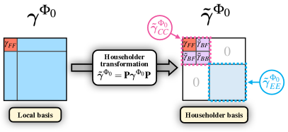
Figure 1: Schematic representation of the Householder transformation on an idempotent 1-RDM of the mean-field state $|\Phi_{0}\rangle$. On the left: 1-RDM in the local basis, where $\gamma_{FF}$ denotes the fragment element. On the right: 1-RDM in the Householder basis, where the two decoupled sectors are delineated, the embedding cluster $\bm{\tilde{\gamma}}_{CC}^{\Phi_{0}}$ in the top left, and the cluster’s environment $\bm{\tilde{\gamma}}_{EE}^{\Phi_{0}}$ in the bottom right.

II.2 Exact fragment embedding for ensembles of states at the non-interacting level

Going beyond the ground state, we will now demonstrate that the Householder transformation can also generate an exact fragment embedding adapted to ground and excited states simultaneously. As ensembles are the original motivation of our approach, we will first provides more details on this new framework. Then we will explain how to adapt the use of the Householder transformation to this new context to design an exact and democratic ensemble embedding at the non-interacting level.

II.2.1 Original motivations: the ensemble framework

In electronic structure calculations, ensemble approaches are usually considered as an appropriate choice to study systems where several low-lying states need to be treated on an equal footing (e.g. in photochemical systems with degenerate states). Indeed, compared to state-specific approaches, ensemble-based methods have two main advantages: i) they provide an unbiased democratic treatment of multiple states, and ii) they are rigorously supported by the ensemble GOK variational principle Gross, Oliveira, and Kohn (1988). To illustrate this, let us assume we are interested in the ground $\ket{\Psi_{0}}$ and first excited state $\ket{\Psi_{1}}$ (with respective energy $E_{0}$ and $E_{1}$) of generic many-electron Hamiltonian $\hat{H}=\hat{h}+\hat{g}$ where $\hat{h}$ and $\hat{g}$ are one- and two-electron operators. Then, the GOK variational principle stipulates that any ensemble energy $E^{\mathbb{w}}$ built from the weighted contribution of any couple of trial states, noted $|\psi_{0}\rangle$ and $|\psi_{1}\rangle$, will always follow

$$E^{\mathbb{w}}=w_{0}\langle\psi_{0}|\hat{H}|\psi_{0}\rangle+w_{1}\langle\psi_{1}|\hat{H}|\psi_{1}\rangle\geq w_{0}E_{0}+w_{1}E_{1},$$ (5)

where the two weights $\mathbf{w}=(w_{0},w_{1})$ fulfill the constraints $w_{0}\geq w_{1}$ and $w_{0}+w_{1}=1$. Here, a strict equality is fulfilled if the trial states correspond to the exact ground and excited states $|\psi_{0}\rangle=|\Psi_{0}\rangle$ and $|\psi_{1}\rangle=|\Psi_{1}\rangle$ of the targeted system. Interestingly, the general definition of the ensemble energy $E^{\mathbb{w}}$ given in Eq. (5) holds true for any type of system, including noninteracting ones (or mean-field ones). In the latter case, one can easily show that the (exact) ensemble energy is a functional of the ensemble 1-RDM noted $\bm{\gamma}^{\mathbf{w}}$ which is defined by

$$\bm{\gamma}^{\mathbf{w}}=w_{0}\bm{\gamma}^{\Phi_{0}}+w_{1}\bm{\gamma}^{\Phi_{1}},$$ (6)

where $\bm{\gamma}^{\Phi_{0}}$ and $\bm{\gamma}^{\Phi_{0}}$ are the 1-RDMs (as defined in Eq. (1)) associated to the exact ground and first excited state $\ket{\Phi_{0}}$ and $\ket{\Phi_{1}}$ of the non-interacting reference system.

The fact that the exact ensemble energy of a non-interacting system can be recovered only from its ensemble 1-RDM is a motivating starting point for the development of an exact fragment embedding for multiple states at the noninteracting level. In this case, the ensemble 1-RDM naturally appears as the new ingredient to be manipulated. However, additional care has to be paid here as ensemble 1-RDMs are generally not idempotent (i.e. $\bm{\gamma}^{\mathbf{w}}\neq(\bm{\gamma}^{\mathbf{w}})^{2}$). Thus, it is not expected that a simple application of the Householder transformation can lead to a block-diagonalization of the matrix (as explained in Ref. Sekaran et al. (2021)). In the following, we will introduce an extension of this approach that can tackle this issue.

II.2.2 Exact fragment embedding using series of Householder transformations

To fulfill the exact block-diagonalization of the non-idempotent ensemble 1-RDM, the strategy we propose consists in applying, not one, but a finite series of Householder transformations. Such a technique is usually employed in tri-diagonalization procedures Householder (1958b, c) as a preprocessing step for computing eigenvalues of symmetric matrices Burden and Faires (2011) (see Appendix A for more details). Concisely, it is performed by applying to a generic matrix $\mathbb{M}$ with a dimension $D$, a product of $D-1$ Householder transformations $\mathbf{Q}=\mathbf{P}^{(1)}\mathbf{P}^{(2)}\dots\mathbf{P}^{(D-1)}$ such that

$$\begin{aligned} \tilde{\mathbb{M}}=\mathbf{Q}^{\dagger}\mathbb{M}\mathbf{Q}\end{aligned}$$ (7)

is a tri-diagonal matrix. In the context of fragment embedding for ensembles, our objective is however a little bit different than tri-diagonalization: we want to reach a block-diagonal form for the ensemble 1-RDM $\bm{\gamma}^{\mathbb{w}}$. To reach this goal, a similar approach may be used in practice but with a truncated number of successive Householder transformations.

To illustrate this, we will first consider the particular case of an ensemble 1-RDM built from only two states: a ground state $\ket{\Phi_{0}}$ and a first excited state $\ket{\Phi_{1}}$ of a given non-interacting system (as given in Eq. (6)). In the eigen-orbital basis of the reference non-interacting Hamiltonian (or mean-field one), the ground state is a single Slater determinant with lowest orbitals doubly-occupied, while the first excited state is given by the HOMO-LUMO orbitals excitation such that

$$\left|\Phi_{1}\right\rangle=\dfrac{1}{\sqrt{2}}\left(\sum_{\sigma=\uparrow,\downarrow}\hat{a}_{N/2+1,\sigma}^{\dagger}\hat{a}_{N/2,\sigma}\right)|\Phi_{0}\rangle.$$ (8)

Starting from the associated ensemble 1-RDM $\bm{\gamma}^{\mathbf{w}}$ expressed in a local orbital basis, we can show that by applying three successive Householder transformations

$$\mathbf{Q}=\mathbf{P}^{(1)}\mathbf{P}^{(2)}\mathbf{P}^{(3)},$$ (9)

the resulting transformed matrix

$$\bm{\tilde{\gamma}}^{\mathbf{w}}=\mathbf{Q}^{\dagger}\bm{\gamma}^{\mathbf{w}}\mathbf{Q},$$ (10)

is block diagonalized with a cluster block fully decoupled form an environment block as exemplified in Fig. 2. As shown in this figure, the dimension of the resulting cluster block is

$$\dim(\bm{\tilde{\gamma}}_{{C}{C}}^{\mathbf{w}})=4,$$ (11)

and we can also mathematically demonstrate (see Appendix C) that the trace of this block is finite with

$$\Tr[\bm{\tilde{\gamma}}_{{C}{C}}^{\mathbf{w}}]=2.$$ (12)

This indicates that the cluster exactly contains $2$ electrons in total (equivalently $4$ electrons if we consider spatial orbitals). A closed cluster containing an integer number of electron reveal that the resulting Householder orbital basis lead to an exact fragment embedding for the two-state ensemble. Indeed, here both ground and excited state factorize into a cluster and environment parts such that

$$|\Phi_{I}\rangle\overset{I=0,1}{=}|\Phi_{0}^{{E}}\rangle|\Phi_{I}^{{C}}\rangle,$$ (13)

where the cluster’s environment $|\Phi_{0}^{{E}}\rangle$ is the same fully-occupied Slater determinant for both states, since they have the same $N/2-1$ fully occupied orbitals. This exact factorization of the two wavefunctions goes along the lines of what was obtained for a single state (see Section II.1). Similarly, the orbital space partitioning allows a straightforward use of regular high-level methods to describe the electronic correlation within the cluster (e.g. in next steps of a DMET procedure).

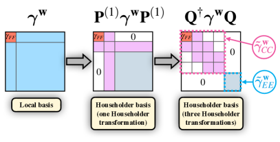
Figure 2: Exact block-diagonalization of a two-state ensemble 1-RDM $\bm{\gamma}^{\mathbb{w}}$ (as defined in Eq. (6)) based on three successive Householder transformations $\mathbf{Q}=\mathbf{P}^{(1)}\mathbf{P}^{(2)}\mathbf{P}^{(3)}$.

The ability to construct an exact fragment embedding for a two-state ensemble marks a promising initial step, prompting inquiry into whether analogous characteristics persist for ensembles with $M>2$ states, where the reference 1-RDM is

$$\mathbb{\gamma}^{\mathbb{w}}=\sum_{I=0}^{M-1}w_{I}\ \mathbb{\gamma}^{\Phi_{I}}.$$ (14)

Numerical and analytical investigations actually revealed that an exact embedding can also be envisioned in this a priori more involved case. However, surprisingly, it turns out that the total number of states $M$ in the ensemble is not the predominant ingredient that will condition the embedding. Indeed, it can be theoretically established that the properties of the final Householder cluster, such as dimensionality (i.e. $\dim(\bm{\tilde{\gamma}}_{{C}{C}}^{\mathbf{w}})$) and the number of electrons it contains (i.e. $\Tr[\bm{\tilde{\gamma}}_{{C}{C}}^{\mathbf{w}}]$), are actually only influenced by the fractionally occupied natural orbital subspace delineated within the reference ensemble 1-RDM $\bm{\gamma}^{\mathbb{w}}$ (as defined in Eq. (14)). Specifically, two pivotal factors of the ensemble 1-RDM will govern the final cluster’s properties: the total count of fractionally occupied natural-orbitals, denoted as $N_{frac}^{orb}$, and the corresponding quantity of electrons, represented as $N_{frac}^{elec}$, inhabiting these natural orbitals. More precisely, we can show that the trace and the dimension of the cluster block $\bm{\tilde{\gamma}}_{{C}{C}}^{\mathbf{w}}$ follow the linear behaviors:

$$\begin{cases}\dim(\bm{\tilde{\gamma}}_{{C}{C}}^{\mathbf{w}})&=2+N_{frac}^{orb}\\ \Tr[\bm{\tilde{\gamma}}_{{C}{C}}^{\mathbf{w}}]&=1+{N_{frac}^{elec}}/{2}.\par\end{cases}$$ (15)

For sake of conciseness, we will provide here a numerical proof of these properties, while directing interested readers to Appendix C for a comprehensive mathematical proof of these behaviors.

To illustrate the laws given in Eq. (15), we have built an artificial ensemble 1-RDM $\gamma^{\mathbb{w}}$, wherein both parameters $N_{frac}^{orb}$ and $N_{elec}^{orb}$ are systematically adjusted to delineate the characteristics of the fractionally occupied natural orbital subspace. Following the specification of these parameters, a series of Householder transformations are applied iteratively on the reference matrix (as defined in Eq. (7)), ceasing when a decoupled cluster block is detected. Subsequently, we evaluate the properties of the resulting cluster (for further technical details of these simulations, see Appendix B). In Fig. 3, we depict the number of Householder transformations necessary to generate an exact decoupling of the cluster along with the variation of the cluster block’s dimension, $\dim(\bm{\tilde{\gamma}}_{{C}{C}}^{\mathbf{w}})$, and its trace, $\Tr[\bm{\tilde{\gamma}}_{{C}{C}}^{\mathbf{w}}]$, with respect to $N_{frac}^{orb}$ (and for different fixed values of $N_{elec}^{orb}=2,4,$ and $6$). As depicted in the top panel of Fig. 2, we see that the number of Householder transformation necessary to generate an independent cluster scales like $1+N_{frac}^{orb}$, and the latter is totally independent from ${N_{frac}^{elec}}$. In the middle panel of Fig. 3, similarly we note that the dimension of the cluster block, $\dim(\bm{\tilde{\gamma}}_{{C}{C}}^{\mathbf{w}})$, only increases with ${N_{frac}^{orb}}$ and not ${N_{orb}^{elec}}$, in accordance with $\dim(\bm{\tilde{\gamma}}_{{C}{C}}^{\mathbf{w}})=2+N_{frac}^{orb}$ as defined in Eq. (15). Conversely, in the bottom panel of Fig. 3, we observe that the electron count within the cluster, represented by $\Tr[\bm{\tilde{\gamma}}_{{C}{C}}^{\mathbf{w}}]$ is steady with the variation of ${N^{orb}_{frac}}$. However, reading vertically the plot, we see that the trace increase linearly with respect to ${N_{frac}^{elec}}$ following the behavior $\Tr[\bm{\tilde{\gamma}}_{{C}{C}}^{\mathbf{w}}]=1+{N_{frac}^{elec}}/{2}$, as defined in Eq. (15). It’s noteworthy that the series of data illustrated in Fig. 3 do not all initiate with the same ${N_{frac}^{orb}}$ value. This disparity stems from the constraint aimed at guaranteeing physically meaningful orbital occupation scenarios, which mandates that ${N_{frac}^{elec}}\geq{N_{frac}^{orb}}$.

The behaviors observed here evidence the possibility to exactly block-diagonalize a general ensemble 1-RDM with the use of a series of Householder transformations. It is a proof that we can build an exact fragment embedding at the non-interacting level for $M$ states as the latter, in the Householder orbital basis, can be exactly factorized in a cluster and environment part as

$$|\Phi_{I}\rangle=|\Phi_{0}^{{E}}\rangle|\Phi_{I}^{{C}}\rangle,\text{ for }I=0,1,\ldots,M-1.$$ (16)

However, this manipulation is not without consequences, as it inevitably leads to an increase in the dimensionality of the cluster, a parameter directly influenced by the quantity of fractionally occupied natural orbitals, $N_{\text{frac}}^{\text{orb}}$ (as detailed in Eq. (15)). Naturally, this behavior may impose limitations on the strategy, especially when $N_{\text{frac}}^{\text{orb}}$ becomes comparable to the size $N$ of the system under study. Such a situation would arise as soon as we consider large ensembles composed of a large number of states decomposed onto a large number of orbitals. The investigation of such exotic situations is left for future work, as our current objective is more motivated by the ambition to target a few low-lying states requiring only a restricted number of orbitals at the non-interacting level.

To conclude this section, we emphasize that so far, we have focused on exact embedding of single-orbital fragments. As discussed in Section III, by contrasting the application of SVD and Householder transformations in the generation of bath orbitals, we can discern the underlying mechanisms driving the expansion of the ensemble embedding cluster’s dimension for fragments of arbitrary size, thereby generalizing the numerical results in Eq. (15). Our interpretations provide compelling evidence that the enlargement of the cluster is a direct result of incorporating fractionally occupied natural orbitals from the ensemble 1-RDM.

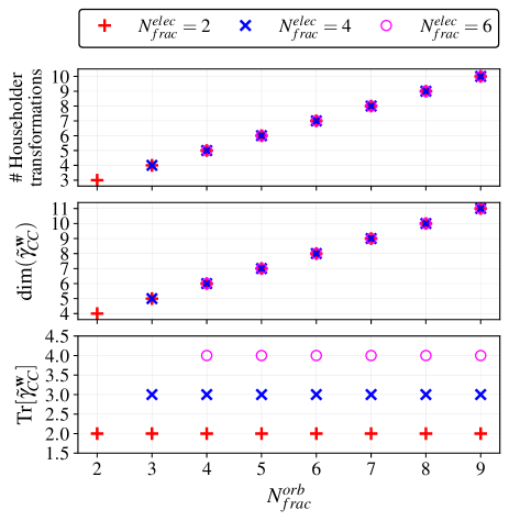
Figure 3: Evolution of the properties of the Householder cluster-block $\bm{\tilde{\gamma}}^{\mathbb{w}}_{CC}$ with the number of fractionally occupied orbital $N_{frac}$. Top panel: the number of Householder transformations required to generate a disentangled Householder cluster-block. Middle panel: dimension of the block. Bottom panel: trace of the block, i.e. number of electrons in the cluster. To produce these results a reference 1-RDM $\bm{\gamma}^{\mathbb{w}}$ is considered where we artificially modulate the $N_{frac}^{orb}$ and $N_{frac}^{elec}$ that defined the fractional occupied orbital space (see Appendix B for practical details).

III Comparison with the DMET bath construction and extension to multi-orbital fragments

In regular (ground-state) DMET Knizia and Chan (2012); Wouters et al. (2016), there are various (equivalent) ways to generate the (one-electron) quantum bath from an idempotent 1-RDM (simply referred to as density matrix in this section) that describes the entire system. One of them relies on the SVD of the fragment’s environment-fragment block Zheng (2018); Li et al. (2023). It has been shown recently Sekaran, Bindech, and Fromager (2023) that this procedure generates the exact same one-electron bath subspace as the Householder transformation (or Block-Householder, if the to-be-embedded fragment contains several spin-orbitals) . In the following, we revisit the DMET bath construction for a non-interacting ensemble and show that, as expected from the previous section, the embedding can be made exact with a limited number (larger than for the ground-state problem) of bath spin-orbitals. The strategy applies also to ensemble mean-field calculations (the so-called ensemble density matrix Hartree–Fock approach in Ref. 43). By analogy with regular DMET, electron correlation can be introduced a posteriori within the embedding cluster, from which local ground- and excited-state properties can be computed, approximately (see Section IV). It should be possible to exactify formally the entire embedding procedure through the ensemble density-functional theory formalism Cernatic et al. (2022), by analogy with the ground-state local potential functional embedding theory Sekaran, Saubanere, and Fromager (2022).

III.1 Ensemble energy within the molecular spin-orbital representation

Let

$$\hat{h}=\sum_{pq}h_{pq}\hat{c}_{p}^{\dagger}\hat{c}_{q}$$ (17)

be the (non-interacting in the present case) second-quantized Hamiltonian written in a given orthonormal basis of localized orbitals (sites for lattice models). Once the Schrödinger equation has been solved for a single electron, i.e.,

$$\hat{h}\left|\kappa\right\rangle=\varepsilon_{\kappa}\left|\kappa\right\rangle,$$ (18)

where $\left|\kappa\right\rangle\equiv\hat{a}_{\kappa}^{\dagger}\left|\rm vac\right\rangle$ corresponds to a molecular spin-orbital with energy $\varepsilon_{\kappa}$ and $\left|\rm vac\right\rangle$ denotes the (zero-electron) vacuum state, we can, on the basis of the many-electron ensemble we want to study, split the one-electron Hilbert space into an even number $N^{\rm In}$ of inactive spin-orbitals $\kappa_{i}$ (the corresponding spatial orbitals are doubly-occupied in all the Slater determinants from which ground- and excited-state wavefunctions are constructed), $N^{\rm Ac}$ actives $\kappa_{a}$ (occupied in some of the Slater determinants from which ground and excited states are described), and the virtuals $\kappa_{r}$ (unoccupied in all the states that belong to the ensemble under study):

$$\begin{aligned} \left\{\left|\kappa\right\rangle\right\}&=\left\{\left|\kappa_{i}\right\rangle\right\}_{1\leq i\leq N^{\rm In}}\oplus\left\{\left|\kappa_{a}\right\rangle\right\}_{N^{\rm In}+1\leq a\leq N^{\rm In}+N^{\rm Ac}}\\ &\quad\quad\oplus\left\{\left|\kappa_{r}\right\rangle\right\}_{r>N^{\rm In}+N^{\rm Ac}}.\end{aligned}$$ (19)

The molecular spin-orbital energies are ordered as follows,

$$\varepsilon_{\kappa_{k}}\leq\varepsilon_{\kappa_{k+1}},$$ (20)

and, by definition,

$$\varepsilon_{\kappa_{i}}<\varepsilon_{\kappa_{a}}<\varepsilon_{\kappa_{r}},\;\forall i,a,r.$$ (21)

The many-electron eigenstates of $\hat{h}$ that form the ensemble have the following structure

$$\left|\Phi_{I}\right\rangle =\left(\hat{\Phi}^{\rm In}\right)^{\dagger}\left(\hat{\Phi}^{\rm Ac}_{I}\right)^{\dagger}\left|\rm vac\right\rangle=\left(\hat{\Phi}^{\rm Ac}_{I}\right)^{\dagger}\left(\hat{\Phi}^{\rm In}\right)^{\dagger}\left|\rm vac\right\rangle$$ (22a)

$$\equiv\left|{\Phi}^{\rm In}{\Phi}^{\rm Ac}_{I}\right\rangle,$$ (22b)

where

$$\left(\hat{\Phi}^{\rm In}\right)^{\dagger}=\prod^{N^{\rm In}}_{i=1}\hat{a}_{\kappa_{i}}^{\dagger}$$ (23)

creates the closed-shell Slater determinant

$$\left|\Phi^{\rm In}\right\rangle=\left(\hat{\Phi}^{\rm In}\right)^{\dagger}\left|\rm vac\right\rangle$$ (24)

that describes the $N^{\rm In}$ inactive electrons to which the regular DMET bath construction will be applied later on. The $\mathcal{N}^{\rm Ac}_{e}$-electron states $\left|\Phi^{\rm Ac}_{I}\right\rangle:=\left(\hat{\Phi}^{\rm Ac}_{I}\right)^{\dagger}\left|\rm vac\right\rangle$, which are a priori not single Slater determinants, unlike $\Phi^{\rm In}$, are constructed from the active spin orbitals whose occupation in $\left|\Phi^{\rm Ac}_{I}\right\rangle$ depends on the state $I$ under consideration within the ensemble:

$$\left|\Phi^{\rm Ac}_{I}\right\rangle\in\left\{\prod^{N^{\rm In}+N^{\rm Ac}}_{a=N^{\rm In}+1}\left(\hat{a}_{\kappa_{a}}^{\dagger}\right)^{n_{\kappa_{a}}}\left|\rm vac\right\rangle\right\},$$ (25)

where $n_{\kappa_{a}}\in\{0,1\}$ and $\sum^{N^{\rm In}+N^{\rm Ac}}_{a=N^{\rm In}+1}n_{\kappa_{a}}=\mathcal{N}^{\rm Ac}_{e}$. From the Hamiltonian representation in the molecular spin-orbital basis,

$$\hat{h} =\sum^{N^{\rm In}}_{i=1}\varepsilon_{\kappa_{i}}\hat{a}_{\kappa_{i}}^{\dagger}\hat{a}_{\kappa_{i}}+\sum^{N^{\rm In}+N^{\rm Ac}}_{a=N^{\rm In}+1}\varepsilon_{\kappa_{a}}\hat{a}_{\kappa_{a}}^{\dagger}\hat{a}_{\kappa_{a}}+\sum_{r>N^{\rm Ac}+N^{\rm In}}\varepsilon_{\kappa_{r}}\hat{a}_{\kappa_{r}}^{\dagger}\hat{a}_{\kappa_{r}}$$ (26a)

$$=:\hat{h}^{\rm In}+\hat{h}^{\rm Ac}+\sum_{r>N^{\rm Ac}+N^{\rm In}}\varepsilon_{\kappa_{r}}\hat{a}_{\kappa_{r}}^{\dagger}\hat{a}_{\kappa_{r}},$$ (26b)

we can finally evaluate the (minimizing GOK Gross, Oliveira, and Kohn (1988)) ensemble energy as follows,

$$E^{\mathbf{w}} =\sum_{I\geq 0}w_{I}\left\langle\Phi_{I}\middle|\hat{h}\middle|\Phi_{I}\right\rangle$$ (27a)

$$=\sum_{I\geq 0}w_{I}\left(\left\langle\Phi_{I}\middle|\hat{h}^{\rm In}\middle|\Phi_{I}\right\rangle+\left\langle\Phi_{I}\middle|\hat{h}^{\rm Ac}\middle|\Phi_{I}\right\rangle\right),$$ (27b)

thus leading to (see Eq. (22a))

$$E^{\mathbf{w}}=\sum_{I\geq 0}w_{I}\left(\left\langle\Phi^{\rm In}\middle|\hat{h}^{\rm In}\middle|\Phi^{\rm In}\right\rangle+\left\langle\Phi^{\rm Ac}_{I}\middle|\hat{h}^{\rm Ac}\middle|\Phi^{\rm Ac}_{I}\right\rangle\right),$$ (28)

or, equivalently,

$$E^{\mathbf{w}}=\sum_{I\geq 0}w_{I}\left(\left\langle\Phi^{\rm In}\middle|\hat{h}\middle|\Phi^{\rm In}\right\rangle+\left\langle\Phi^{\rm Ac}_{I}\middle|\hat{h}\middle|\Phi^{\rm Ac}_{I}\right\rangle\right).$$ (29)

From the above energy expression, we first realize that the regular DMET algorithm (or, equivalently, the Householder transformation Sekaran, Bindech, and Fromager (2023)) can be used straightforwardly to evaluate the inactive part of the ensemble energy (first term on the right-hand side of Eq. (29)), simply because it is described by a single Slater determinant. Increasing the embedding cluster’s size and the number of electrons it contains, in order to describe the active part of the ensemble energy (second term on the right-hand side of Eq. (29)), will provide a rationale for the conclusions drawn in Section II.2.2 (see Eq. (15)). This is discussed in the next section.

III.2 Embedding of the inactive energy and enlargement of the embedding cluster with the actives

We now consider an alternative decomposition of the one-electron Hilbert space into the to-be-embedded fragment spin-orbital subspace $F$ of dimension $L_{F}$ and its complement $\overline{F}$, which corresponds to the complete and true environment of the fragment in the system under study:

$$\left\{\left|\kappa_{i}\right\rangle\right\}\oplus\left\{\left|\kappa_{a}\right\rangle\right\}\oplus\left\{\left|\kappa_{r}\right\rangle\right\}=F\oplus\overline{F}.$$ (30)

Unlike in Section II, we consider the more general case where multiple (spatial) orbitals can be embedded (i.e., $L_{F}>2$). On that basis, a third (so-called embedding) representation can be constructed by applying the regular DMET bath construction to the single-determinantal inactive wavefunction $\Phi^{\rm In}$, thus leading to the following decomposition (see, for example, Ref. 35 for further details),

$$F\oplus\overline{F}=\underset{C^{\rm In}}{\underbrace{F\oplus B^{\rm In}}}\oplus\mathcal{E}^{\rm In},$$ (31)

where the one-electron bath subspace $B^{\rm In}$, whose dimension equals that of the fragment ($\dim B^{\rm In}=\dim F=L_{F}$), will be referred to as inactive bath because it is constructed from $\Phi^{\rm In}$ or, more precisely, from the (one-electron reduced) density matrix ${\bm{\gamma}}^{\rm In}$ of $\Phi^{\rm In}$ written in the original localized representation (see Eq. (17)):

$${\gamma}^{\rm In}_{pq}=\left\langle\Phi^{\rm In}\middle|\hat{c}_{p}^{\dagger}\hat{c}_{q}\middle|\Phi^{\rm In}\right\rangle.$$ (32)

Indeed, a simple basis of $B^{\rm In}$ (which can be orthonormalized via the SVD of the $\overline{F}F$ block of ${\bm{\gamma}}^{\rm In}$, for example) is generated as follows Sekaran, Bindech, and Fromager (2023),

$$B^{\rm In}=\left\{\sum_{q\in\overline{F}}\gamma^{\rm In}_{pq}\hat{c}^{\dagger}_{q}\left|{\rm vac}\right\rangle\right\}_{p\in F}.$$ (33)

Localized and embedding representations can be connected through a unitary transformation (that applies to the entire one-electron Hilbert space),

$$\bm{\gamma}^{\rm In}\rightarrow\tilde{\bm{\gamma}}^{\rm In}=\left(\mathcal{U}^{\rm In}\right)^{\dagger}\bm{\gamma}^{\rm In}\mathcal{U}^{\rm In},$$ (34)

which, by construction, leaves the fragment unchanged and, as a consequence of Eq. (33) and the idempotency of ${\bm{\gamma}}^{\rm In}$ Sekaran, Bindech, and Fromager (2023), ensures the strict disentanglement of the inactive embedding cluster $C^{\rm In}$ (fragment+inactive bath) from its environment $\mathcal{E}^{\rm In}$ (see Eq. (31)), i.e.,

$$\tilde{\gamma}^{\rm In}_{pq}\overset{p\in\mathcal{E}^{\rm In}}{\underset{q\in C^{\rm In}}{=}}0.$$ (35)

It also guarantees that the inactive cluster contains as many electrons as the number of spin-orbitals in the fragment:

$$\sum_{p\in C^{\rm In}}\tilde{\gamma}^{\rm In}_{pp}=L_{F}.$$ (36)

Consequently, the inactive part of the ensemble energy (first term on the right-hand side of Eq. (29)) can be evaluated in the embedding representation as follows (we use real algebra for simplicity),

$$\left\langle\Phi^{\rm In}\middle|\hat{h}\middle|\Phi^{\rm In}\right\rangle =\Tr\left[h\bm{\gamma}^{\rm In}\right]=\Tr\left[\tilde{h}\bm{\tilde{\gamma}}^{\rm In}\right]$$ (37a)

$$=\sum_{pq\in C^{\rm In}}\tilde{h}_{pq}\tilde{\gamma}^{\rm In}_{pq}+\sum_{pq\in\mathcal{E}^{\rm In}}\tilde{h}_{pq}\tilde{\gamma}^{\rm In}_{pq},$$ (37b)

where $h\equiv\left\{h_{pq}\right\}$ and $\tilde{h}=\left(\mathcal{U}^{\rm In}\right)^{\dagger}h\mathcal{U}^{\rm In}$. As the idempotency of $\bm{\gamma}^{\rm In}$ implies that of its $C^{\rm In}C^{\rm In}$ block (because of Eq. (35)), it comes from Eq. (36) that the inactive cluster part of the energy (first term on the right-hand side of Eq. (37b)) can be evaluated from a single-determinantal $L_{F}$-electron wavefunction $\Phi^{C^{\rm In}}$. Note that, in practice, $\Phi^{C^{\rm In}}$ would be determined by diagonalizing the projection of $\hat{h}$ onto the $L_{F}$-electron Fock subspace that is generated from the inactive embedding cluster. In this representation, $\Phi^{C^{\rm In}}$ is written as a multi-determinantal wavefunction. In practical DMET computations, the electronic repulsion within the fragment (possibly the bath too) would also be taken into account, thus leading, in this case, to an (approximate) embedding scheme where $\Phi^{C^{\rm In}}$ would become a correlated wavefunction. Returning to the non-interacting case, in which the embedding is exact, we finally obtain the following expression for the inactive energy,

$$\left\langle\Phi^{\rm In}\middle|\hat{h}\middle|\Phi^{\rm In}\right\rangle=\left\langle\Phi^{C^{\rm In}}\middle|\hat{h}\middle|\Phi^{C^{\rm In}}\right\rangle+\sum_{pq\in\mathcal{E}^{\rm In}}\tilde{h}_{pq}\tilde{\gamma}^{\rm In}_{pq}.$$ (38)

Let us now elaborate on the inactive embedding cluster contribution (first term on the right-hand side of Eq. (38)). In the corresponding diagonalizing one-electron representation, the inactive embedding cluster subspace is split into occupied-in-$\Phi^{C^{\rm In}}$ spin-orbitals (which belong to the inactive subspace) and unoccupied-in-$\Phi^{C^{\rm In}}$ spin-orbitals, which belong to the active+virtual subspace. Note that, so far, we have simply applied the regular DMET approach to the inactive electrons. In order to recover the active contributions to the ensemble energy (second term on the right-hand side of Eq. (29)), we need to complement the inactive embedding cluster with the active spin-orbital subspace (from which the projection onto the inactive cluster is removed, via the projection operator $\hat{P}_{C^{\rm In}}$). Thus, we obtain an enlarged and definitive embedding cluster subspace

$${C}=C^{\rm In}\oplus\left\{\left(\hat{\mathds{1}}-\hat{P}_{C^{\rm In}}\right)\left|\kappa_{a}\right\rangle\right\}_{N^{\rm In}+1\leq a\leq N^{\rm In}+N^{\rm Ac}}$$ (39)

from which the exact ensemble energy can be evaluated as follows (note that the weights sum up to 1),

$$E^{\mathbf{w}}=\sum_{I\geq 0}w_{I}\left\langle\Phi_{I}^{C}\middle|\hat{h}\middle|\Phi_{I}^{C}\right\rangle+\sum_{pq\in\mathcal{E}^{\rm In}}\tilde{h}_{pq}\tilde{\gamma}^{\rm In}_{pq},$$ (40)

where, with the notation of Eq. (22b), the embedded ground and excited states read

$$\left|\Phi_{I}^{{C}}\right\rangle\equiv\left|\Phi^{{C}^{\rm In}}\Phi_{I}^{\rm Ac}\right\rangle.$$ (41)

As readily seen from Eqs. (31) and (40), the cluster ensemble energy (first sum on the right-hand side of Eq. (40)) is the only energy contribution we need to evaluate (variationally) to retrieve ground- and excited-state properties (i.e., reduced density matrices) within the fragment subspace, which is orthogonal to the inactive embedding cluster’s environment subspace $\mathcal{E}^{\rm In}$. This is simply achieved by diagonalizing the projection of the Hamiltonian $\hat{h}$ onto the space of Slater determinants that is generated by distributing $L_{F}+\mathcal{N}^{\rm Ac}_{e}$ electrons (the first $L_{F}$ electrons come from the inactive embedding cluster, as readily seen from Eq. (41)) among $2L_{F}+N^{\rm Ac}$ spin-orbitals (the first $2L_{F}$ spin-orbitals come from the fragment and the inactive bath, as readily seen from Eqs. (31) and (39)). As we did not specify the number $L_{F}$ of fragment spin-orbitals that are embedded, we generalize the key result of Eq. (15), which is recovered in the particular case where a single (spatial) orbital is embedded, i.e., $L_{F}=2$. In this case, if we use the notations of Eq. (15), the dimension of the complete embedding cluster $C$ (including both spin states) is $4+N^{\rm Ac}=2(2+N_{frac}^{orb})$, and the total number of electrons in the cluster is $2+\mathcal{N}^{\rm Ac}_{e}=2(1+(N_{frac}^{elec}/2))$.

III.3 Summary and key conclusions of the comparison

The characteristics of the (single-orbital fragment) embedding cluster (i.e., its dimension and the number of electrons it contains), as constructed mathematically in Section II.2.2 from successive ensemble density matrix functional Householder transformations, have been recovered from a different perspective, by extending the regular DMET bath construction to (GOK) ensembles. For that purpose, we first embedded a fragment (of arbitrary dimension $L_{F}$) in the presence of the inactive electrons, thus leading to an inactive embedding cluster of dimension $2L_{F}$ that contains $L_{F}$ electrons. The latter cluster was then complemented by $N^{\rm Ac}$ active spin-orbitals in which $\mathcal{N}^{\rm Ac}_{e}$ electrons are originally (i.e., at the full-size level of calculation) distributed to create the ensemble under study. We finally obtain a cluster of dimension $2L_{F}+N^{\rm Ac}$ (total number of spin-orbitals) that contains $L_{F}+\mathcal{N}^{\rm Ac}_{e}$ electrons. The procedure is exact for non-interacting (or mean-field) ensembles and applies to both single- and multi-orbital fragment embeddings. As discussed in further details in Section IV, its practical extension to the interacting problem (for which the embedding becomes actually useful) consists in introducing the electronic repulsion within the cluster, by analogy with regular ground-state DMET. The embedding becomes approximate in this case.

Let us finally stress that, even though the present DMET-like construction of the ensemble embedding cluster is simpler in its mathematical formulation than the composition of Householder transformations (as introduced in Section II.2), the latter has the main advantage (that is not exploited in the present work) of providing automatically a complete orthonormal embedding basis for the full one-electron Hilbert space (i.e., for the embedding cluster and its environment). Future developments where, for example, multi-reference perturbation theory could be applied on top of the embedding calculation Sekaran et al. (2021) (where the cluster is treated as a closed system), in order to recover correlations that are external to the cluster, would obviously benefit from this feature.

IV Applications: A SINGLE-SHOT EMBEDDING STRATEGY FOR TWO-STATE ENSEMBLES

IV.1 General description of the method

In the following, we present a first step toward practical implementations of fragment embedding for multiple states. While the findings of numerical study in Section II.2.2 and the above comparison with DMET allude to the possibility of developing a general scheme for targeting an arbitrary number of states, we propose in this section a simple strategy for calculating the energies of ground and first excited singlet states, inspired by the single-shot embedding from DMET-like methods Wouters et al. (2016); Sekaran et al. (2021); Yalouz et al. (2022).

In essence, the strategy consists of utilizing the bath orbitals of the noninteracting Householder cluster as the building blocks of the many-electron basis for correlated embedding cluster wavefunctions. For each fragment in the local basis, the bath orbitals are extracted with the previously described technique of applying successive Householder transformations on the ensemble 1-RDM until block-diagonalization. Afterwards, the embedding Hamiltonian $\hat{H}^{C}$ is constructed by projecting the many-electron Hamiltonian $\hat{H}$ into the Hilbert space of the “fragment+bath" cluster block. In DMET, different versions of $\hat{H}^{C}$ are possible depending on the extent of electron interactions. In the so-called Interacting Bath (IB) formalism, electron interactions appear in both the fragment and bath orbitals, while in the Noninteracting Bath (NIB) formalism, electrons interact only on the fragment Wouters et al. (2016); Wouters, A. Jiménez-Hoyos, and KL Chan (2017); Sekaran et al. (2021); Marécat and Saubanère (2023). In our strategy, we use the IB formalism. In addition, electron interactions between the Householder cluster and the occupied orbitals inside the Householder environment are incorporated in a mean-field way into the one-electron part of $\hat{H}^{C}$. At this point, one may proceed to compute the correlated cluster wavefunctions $|\Psi_{I}^{C}\rangle$ by diagonalizing $\hat{H}^{C}$ with a high-level wavefunction method, in our case the Full Configuration Interaction (FCI) method. However, it is usually observed that local orbital occupations on fragments change drastically when introducing electron interactions inside the cluster. As a consequence, the total number of electrons when summed up from different fragments may not match the true number of electrons in the whole system. A simple solution in DMET is to optimize the global number of electrons by adding a chemical potential $\mu$ on the fragment, thereby enabling the fluctuation of electrons between the fragment and bath in each embedding cluster Wouters et al. (2016); Wouters, A. Jiménez-Hoyos, and KL Chan (2017). Here, we adopt a similar approach, with a slightly more flexible optimization scheme. For each fragment, with orbital indexed "$p$", we solve the following Schrödinger equation,

$$\left(\hat{H}^{C_{p}}-\mu_{p}\hat{n}_{p}\right)|\Psi_{I}^{C_{p}}\rangle=E_{I}^{C_{p}}|\Psi_{I}^{C_{p}}\rangle,$$ (42)

to obtain the correlated cluster wavefunctions $|\Psi_{I}^{C_{p}}\rangle$. In the above equation, $\mu_{p}$ is the chemical potential and ${\hat{n}_{p}=\sum_{\sigma=\uparrow,\downarrow}\hat{c}^{\dagger}_{p,\sigma}\hat{c}_{p,\sigma}}$ the density operator on fragment $p$, and $E_{I}^{C_{p}}$ is the cluster energy (not used in the final energy evaluations). The chemical potentials $\{\mu_{p}\}_{p=1}^{L}$, which are in our calculations allowed to differ across fragments, are adjusted to correct for the right total number of electrons in both the ground and the first excited state, by minimizing the following cost function,

$${\rm CF}(\{\mu_{p}\})=\sum_{I=0,1}\left(\sum_{p=1}^{L}\langle\Psi_{I}^{{C}_{p}}(\mu_{p})|\hat{n}_{p}|\Psi_{I}^{{C}_{p}}(\mu_{p})\rangle-N\right)^{2}.$$ (43)

After the optimization of chemical potentials, the 1- and the 2-RDMs of the ground and excited state wavefunctions of local clusters are assembled to estimate the total energies and other properties of the complete system. For the calculation of energies, we make use of the so-called democratic partitioning approach, which has been extensively discussed in previous works on DMET and related orbital-based quantum embedding methods Wouters et al. (2016); Wouters, A. Jiménez-Hoyos, and KL Chan (2017); Nusspickel, Ibrahim, and Booth (2023). In brief, the electronic energy for each individual state is calculated as

$$E_{I}=\sum_{pq}h_{pq}D_{pq}^{\Psi_{I}}+\sum_{pqrs}g_{pqrs}\Gamma_{pqrs}^{\Psi_{I}},$$ (44)

where $h_{pq}$ and $g_{pqrs}$ are the one- and two-electron integrals in the local basis, and $D_{pq}^{\Psi_{I}}$ and $\Gamma_{pqrs}^{\Psi_{I}}$ are the spin-free 1- and 2-RDMs, respectively. The latter are estimated from embedding calculations on different fragments in a “democratic" fashion as follows,

$$D_{pq}^{\Psi_{I}}=\dfrac{1}{2}\sum_{x=p,q}\,\sum_{\sigma=\uparrow,\downarrow}\langle\Psi_{I}^{C_{x}}|\hat{c}^{\dagger}_{p,\sigma}\hat{c}_{q,\sigma}|\Psi_{I}^{C_{x}}\rangle,$$ (45)

$$\Gamma_{pqrs}^{\Psi_{I}}=\dfrac{1}{4}\sum_{x=p,q,r,s}\,\sum_{\sigma,\sigma^{\prime}=\uparrow,\downarrow}\langle\Psi_{I}^{C_{x}}|\hat{c}^{\dagger}_{p,\sigma}\hat{c}^{\dagger}_{q,\sigma^{\prime}}\hat{c}_{s,\sigma^{\prime}}\hat{c}_{r,\sigma}|\Psi_{I}^{C_{x}}\rangle.$$ (46)

In ab initio systems, the nuclear repulsion energy (a state-independent term) is added to the electronic energies in Eq. (44).

We apply this two-state ensemble embedding strategy in the computation of energy curves in two simple illustrative examples, the first one being a finite Hubbard lattice model, and the second one an ab initio system of Hydrogen atoms. For benchmarking the results of embedding calculations, the FCI approach was used to extract energy levels of ground and first-excited states. In our calculations, the construction of fermionic creation and annihilation operators, and the subsequent construction and diagonalization of FCI and embedding Hamiltonians were carried out using the python package QuantNBody Yalouz, Gullin, and Sekaran (2022).

IV.2 Hubbard ring with site potential asymmetry and bold length alternation

The first system on which we apply our embedding strategy is a Hubbard-like ring with an alternating hopping term and different local orbital energies on odd and even sites (see the top panel of Figure 4 for a sketch of the model). The model Hamiltonian for the ring reads as

$$\begin{aligned} \hat{H}&=-\sum_{p=1}^{L}t_{p}\sum_{\sigma=\uparrow,\downarrow}(\hat{c}^{\dagger}_{p,\sigma}\hat{c}_{p+1,\sigma}+\hat{c}^{\dagger}_{p+1,\sigma}\hat{c}_{p,\sigma})\\ &+U\sum_{p=1}^{L}\hat{n}_{p,\uparrow}\hat{n}_{p,\downarrow}\>+\>\epsilon\sum_{p=1}^{L}(-1)^{p}\hat{n}_{p},\end{aligned}$$ (47)

where

$$t_{p}=\begin{cases}t_{1}&\text{if }p\text{ is odd}\\ t_{2}&\text{if }p\text{ is even}\end{cases}$$ (48)

are the hopping terms, $U$ is the local electronic repulsion, $\epsilon$ is the local orbital energy, $\hat{n}_{p,\sigma}=\hat{c}^{\dagger}_{p,\sigma}\hat{c}_{p,\sigma}$ is the occupation number operator for spin $\sigma$ on site $p$, and $\hat{n}_{p}=\sum_{\sigma=\uparrow,\downarrow}\hat{n}_{p,\sigma}$ is the total occupation number operator on site $p$. In our FCI and embedding calculations, we chose the model with $L=8$ sites and $N=8$ electrons in total. To enforce the ring geometry, periodic boundary conditions ($\hat{c}^{\dagger}_{L+1,\sigma}=\hat{c}^{\dagger}_{1,\sigma}$) were imposed in Eq. (47). The ratio $t_{2}/t_{1}$, which controls the electron delocalization between the four “dimers” in the ring, is the key parameter of study in this model. The $t_{2}/t_{1}\ll 1$ regime represents the bond breaking scenario, where the molecule turns into four separate dimers, while $t_{2}/t_{1}\gg 1$ represents a molecule with strong overlap between dimers. An interesting feature of this model is a very close avoided crossing between the ground and first excited states occurring at $t_{2}/t_{1}=1$ for $U=2t_{1}$ and $\epsilon=0.5t_{1}$, where the ground and first excited state energies differ as $E_{1}-E_{0}\approx 3.55\times 10^{-2}t_{1}$ (see also the inset on Figure 4). Indeed, around an avoided crossing, the eigenstates of a non-interacting system usually undergo non-trivial mixing when electron interactions are switched on, which makes the present model a perfect test example for our method.

Turning to the discussion of embedding calculations, in the first step of the process, we solve the noninteracting electron problem, which is, in the present case, the tight-binding ring ($U=0$ in Eq. (47)). From the molecular orbitals of the tight-binding ring, we then build the equiensemble 1-RDM (where $w_{0}=w_{1}=1/2$) of the ground and first excited noninteracting states in the lattice site basis, which is a convenient and commonly used orthonormal basis for the extraction of bath orbitals in lattice models. As explained in Section II.2.2, the application of three successive Householder transformations on the 1-RDM in the lattice site basis produces a disentangled cluster with three bath orbitals connected to the fragment, which are used to build the correlated clusters in subsequent embedding calculations. After obtaining the bath orbitals, we perform single-shot embedding calculations with the strategy described in Section IV.1. The bottom panel of Figure 4 displays the embedding and FCI energies for the ground and first excited states of the interacting ($U=2t_{1}$) ring, for different values of $t_{2}$ (at $t_{1}=1$). We observe that embedding results are in very good agreement with FCI energies for both states, especially in the region of the avoided crossing. Surprisingly, we also observe that there is no chemical potential tuning necessary to optimize the global number of electrons as long as the mean-field description of electron interactions between the correlated embedding cluster and cluster’s environment $|\Phi_{0}^{{E}}\rangle$ are properly included in embedding calculations (interestingly, the same observation was reported by Marécat et al. in the application of their self-consistent embedding scheme on the 1D Hubbard model Marécat et al. (2023)). Moreover, we also report that any variations of ensemble weights in the range $0<(w_{0},w_{1})<1$ (keeping in mind that they sum up to $1$) had no discernible differences in the final evaluation of energies from embedding clusters.

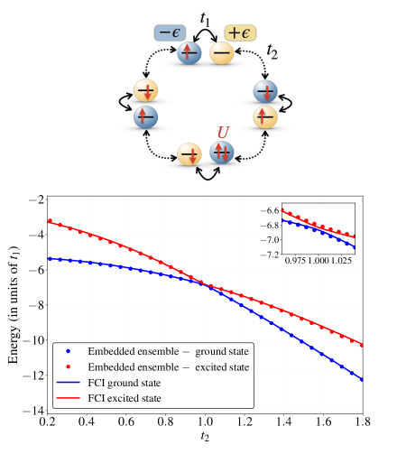
Figure 4: Top panel: A schematic picture of the Hubbard ring model system. Bottom panel: The FCI ground and first excited singlet states (blue, and red lines respectively), and embedding results for the ground and first excited state (blue and red dot markers, respectively) for the Hubbard ring model at $U=2$, $\epsilon=1/2$, $t_{1}=1$ and different values of $t_{2}$.

IV.3 System of hydrogen atoms

Figure 5: Top panel: A schematic picture of the system of Hydrogen atoms by Tran et al. Tran, Van Voorhis, and Thom (2019). Bottom: Dissociation curves of the FCI ground and first excited singlet states (blue and red lines, respectively), and embedding results for the ground and first excited state (blue and red markers, respectively) for the system of Hydrogen atoms. The embedding results are plotted with and without chemical potential optimization (dot ($\bullet$) and cross ($\times$) markers, respectively).

For our second example, we have chosen an ab initio system comprising an arrangement of six hydrogen atoms, which was originally used by Tran et al. in their work on extending DMET to excited states Tran, Van Voorhis, and Thom (2019). Similarly to what we had before in the Hubbard ring model, this system also exhibits an avoided crossing, making it an appealing choice for a complementary study to a model system. For an image of the ab initio system, see the top panel of Figure 5.

The starting mean-field description of the full system was obtained from Restricted Hartree-Fock (RHF) calculations, from which we extracted the molecular orbitals for building the ensemble 1-RDM. The self-consistent iterations of RHF scheme, together with the calculation of one- and two-electron integrals, were carried out with Psi4 python package Smith et al. (2020), using the STO-3G orbital basis set. Unlike in previous example, the construction of a local and orthonormal orbital basis had to be carried out before one could delineate fragments for embedding calculations. This additional preprocessing step of orbital localization is necessary for all ab initio systems, with different procedures employed in practice (for instance, see Ref. Koridon et al. (2021) and reference therein). For this system, we employed Löwdin’s method to build the symmetrically Orthogonalized Atomic Orbitals (OAOs) Löwdin (1950); Carlson and Keller (1957); Mayer (2002). The OAOs are simple to obtain, and are designed to resemble as closely as possible the atomic orbitals of a chemical system, in our case the $1s$ orbitals around Hydrogen atoms. After localization, the mean-field ensemble 1-RDM was constructed, where we again chose the equiensemble weight values. Then, we ran embedding calculations for different intermolecular distances (denoted by $\mathbf{r}$), studying the dissociation of the hydrogen arrangement into three separate molecules. Concerning the effect of the variation of ensemble weights, we report the same observations as in the Hubbard ring. In contrast to the ring, we observe that embedding calculations in the system of hydrogen atoms are amenable to the change in chemical potential. However, as shown in the bottom panel of Figure 5, the embedding results are in excellent agreement with FCI values for both ground and excited states, even in the region near avoided crossing (in between $\mathbf{r}\approx 0.66$Å  and $\mathbf{r}\approx 0.72$Å, see the inset in Figure 5), and the effect of chemical potential optimization on the estimated energies is almost inconsequential. As a final point, in comparison to the state-specific approach of Tran et al (see Figure 2 in Ref. Tran, Van Voorhis, and Thom (2019)), our strategy produced just as good results for all values of $\mathbf{r}$ considered. While in their case, bath orbitals for each individual state are computed from separate SCF calculations, in our strategy we rely on the bath orbitals from a single SCF calculation for embedding all states simultaneously which seems to be less costly.

V Conclusion and perspectives

In the present paper we have tackled the challenge of describing electronic excited states using the methodology of quantum embedding. While the majority of previous studies exploring the feasibility of embedding excited states have focused on state-specific strategies, we embarked in this work in the direction of an embedding strategy for multiple (i.e. ground and excited) states, guided by the recent developments in DMET.

In the first part of the paper, we touched upon the theoretical aspects of fragment embedding, beginning with a short review of DMET and the use of Householder transformation as the key ingredient in the clusterization of the ground-state 1-RDM, enabling the optimal orbital-space partitioning at the mean-field level of electronic structure description. While the idempotency property of 1-RDMs, which is of key importance in ground-state DMET, is lost when moving to ensembles of states, we have shown that an exact clusterization for ensembles is still achievable through the application of a finite number of successive Householder transformations on ensemble 1-RDMs. In the particular case of the two-state ensemble consisting of the linear combination of ground and singly-excited mean-field states, we have shown that the application of three Householder transformations strictly block-diagonalizes the ensemble 1-RDM, giving rise to an enlarged, but still decoupled cluster, containing a finite number of bath orbitals and an integer number of electrons. We also inquired into the possibility of embedding larger-sized ensembles, which we supported by numerical investigations. The latter have shown that a decoupled cluster can also be obtained in more involved scenarios. Precisely, we demonstrated that the Householder cluster size scales linearly with the size of the fractionally-occupied natural orbital subspace in the ensemble 1-RDM, while the number of electrons inside the cluster scales linearly with the number of electrons, inhabiting these fractionally-occupied natural orbitals. These results were also corroborated by rigorous mathematical proofs in the single-orbital fragment case. A rationalization and a formal extension of the approach to the multi-orbital case have finally been obtained by extending the conventional DMET bath construction to GOK ensembles.

In the second part of this work, we presented an implementation of a single-shot embedding strategy for description of the energies of ground and first-excited states in finite systems. Test calculations of energy curves on two illustrative examples have demonstrated that embedding multiple states is a very relevant strategy, especially when different states become increasingly closer in energy and as such are best treated in an unbiased manner. The very strong agreement of embedding and FCI results in the case of system of hydrogen atoms is also very promising, and tempts further exploration of the ensemble embedding in other quantum chemistry applications, like, for example, describing conical intersections, and dissociations of heteroatomic molecules.

In summary, we demonstrated the feasibility of embedding multiple states by repurposing the Householder transformation in a straightforward manner to generate additional bath orbitals in generally non-idempotent ensemble 1-RDMs. The variety of insights, produced in this work begets new questions and considerations for improvements. Firstly, let us mention the prospect of extending the single-shot embedding strategy to more than two states. In this study we relied on extrapolating the exact ensemble emedding with a single HOMO-LUMO excitation in the noninteracting limit, to target the ground and first excited states of interacting systems. Although the aforementioned numerical investigations and the comparison with DMET suggested that embedding ensembles with more excitations is plausible, whether the present strategy would by analogy produce reasonable results for the second and higher excited states is, though fascinating to contemplate, a difficult question which we intend to address in future work. In a different direction, making the embedding self-consistent would be one of the next logical steps. As mentioned in Section III, combining many-electron ensembles with local potential functional embedding theory Sekaran, Saubanere, and Fromager (2022); Yalouz et al. (2022) would be an intriguing route to explore. In the perspective of ensemble density functional theory Cernatic et al. (2022), the embedding would become in-principle exact as both the embedding cluster and the reference full-size noninteracting (Kohn–Sham) system would reproduce the exact ensemble density (i.e., the ensemble occupation of the localized orbitals in the present context). Additionally, we stress that the current implementation was developed only for single-orbital fragments. It would be interesting to investigate whether the application of block-Householder transformations Rotella and Zambettakis (1999); Sekaran et al. (2021); Yalouz et al. (2022); Sekaran, Bindech, and Fromager (2023) can be re-used for multi-orbital fragment embedding in ensembles. Unlike in the standard DMET bath construction (or its extension to ensembles, as also discussed in this work), such transformations would automatically provide a complete orthonormal basis of the full one-electron Hilbert space (i.e., for the embedding cluster and its environment). That basis could be exploited in post-DMET treatments for recovering correlations that are external to the cluster, for example Sekaran et al. (2021). As a final remark, excited states are not the only domain where the problem of non-idempotent density matrices occurs. The same issue arises, for example, in the description of ground-state embedding with correlated bath orbitals, where the 1-RDM in the natural orbital basis is non-idempotent, and for this reason, we strongly believe that the clusterization approach elaborated here will be useful in that context.

Conflict of interest

The authors declare that they have no conflict of interest.

Data availability

The data that support the findings of this study are available from the corresponding author upon reasonable request.

Appendix A Mathematical details of the tri-diagonalization by Householder transformations

Let $\bm{\gamma}$ be a symmetric matrix with dimension $L$. Then, for every ${1\leq i\leq L-2}$, we consider the following change of basis,

$$\bm{\tilde{\gamma}}^{(i+1)}={\mathbf{Q}^{(i)\,\dagger}}\bm{\gamma}\mathbf{Q}^{(i)},$$ (49)

where

$$\mathbf{Q}^{(i)}=\mathbf{P}^{(1)}\mathbf{P}^{(2)}\dots\mathbf{P}^{(i)},$$ (50)

and $\mathbf{P}^{(i)}$ are individual Householder transformations. The latter are defined for $1\leq i\leq L-2$ as follows,

$$\mathbf{P}^{(i)} =\mathbf{I}-2\mathbf{v}^{(i)}\mathbf{v}^{(i)\,\dagger}$$ (51)

where $\mathbf{I}$ is the $L\times L$ identity matrix, and $\mathbf{v}^{(i)}$ is the $i$-th Householder vector, whose elements are given by

$$\mathbf{v}^{(i)} =\begin{bmatrix}v^{(i)}_{1}\\ v^{(i)}_{2}\\ \vdots\\ v^{(i)}_{L}\\ \end{bmatrix},$$ (52)

where

$$v_{1\leq j\leq i}^{(i)}=0,$$ (53)

$$v_{i+1}^{(i)}=\dfrac{\tilde{\gamma}_{i+1,i}^{(i)}-\xi^{(i)}}{2r^{(i)}},$$

$$v_{i+2\leq j\leq L}^{(i)}=\dfrac{\tilde{\gamma}_{j,i}^{(i)}}{2r^{(i)}},$$

and

$$\xi^{(i)}=-sgn\left(\tilde{\gamma}_{i+1,i}^{(i)}\right)\sqrt{\sum_{j=i+1}^{L}\left(\tilde{\gamma}_{j,i}^{(i)}\right)^{2}},$$ (54)

$$r^{(i)}=\sqrt{\dfrac{1}{2}\left(\left(\xi^{(i)}\right)^{2}-\tilde{\gamma}_{i+1,i}^{(i)}\xi^{(i)}\right)}.$$

Starting with $\bm{\tilde{\gamma}}^{(1)}=\bm{\gamma}$, the formulae in Eqs. (53) and (54) can be used to systematically construct, for every step $i$, the Householder transformation $\mathbf{P}^{(i)}$ from the matrix elements of $\bm{\tilde{\gamma}}^{(i)}$, until reaching the fully tri-diagonal matrix $\bm{\tilde{\gamma}}^{(L-1)}$. Given these definitions, one can show that the product of successive Householder transformations $\mathbf{Q}^{(i)}$, is unitary. This follows from the fact that each Householder vector $\mathbf{v}^{(i)}$ is normalized (see Eqs. (53) and (54)),

$$\begin{aligned} \mathbf{v}^{(i)\,\dagger}\mathbf{v}^{(i)}&=\dfrac{(\tilde{\gamma}_{i+1,i}^{(i)}-\xi^{(i)})^{2}-\sum_{j>i+1}^{L}(\tilde{\gamma}_{j,i}^{(i)})^{2}}{4(r^{(i)})^{2}}\\ &=\dfrac{\sum_{j=i+1}^{L}(\tilde{\gamma}_{j,i}^{(i)})^{2}-2\tilde{\gamma}_{i+1,i}^{(i)}\xi^{(i)}+(\xi^{(i)})^{2}}{4(r^{(i)})^{2}}\\ &=\dfrac{2\left((\xi^{(i)})^{2}-\gamma_{i+1,i}^{(i)}\xi^{(i)}\right)}{4(r^{(i)})^{2}}=\dfrac{{4(r^{(i)})^{2}}}{{4(r^{(i)})^{2}}}=1,\end{aligned}$$ (55)

and hence, according to Eqs. (51), and (55), every Householder transformation $\mathbf{P}^{(i)}$ is unitary and Hermitian,

$$\begin{aligned} \mathbf{P}^{(i)\,\dagger}\mathbf{P}^{(i)}&=\mathbf{P}^{(i)}\mathbf{P}^{(i)\,\dagger}=\mathbf{P}^{(i)}\mathbf{P}^{(i)}\\ &=\left(\mathbf{I}-2\mathbf{v}^{(i)}\mathbf{v}^{(i)\,\dagger}\right)\left(\mathbf{I}-2\mathbf{v}^{(i)}\mathbf{v}^{(i)\,\dagger}\right)\\ &=\mathbf{I}-4\mathbf{v}^{(i)}\mathbf{v}^{(i)\,\dagger}+4\mathbf{v}^{(i)}\left(\mathbf{v}^{(i)\,\dagger}\mathbf{v}^{(i)}\right)\mathbf{v}^{(i)\,\dagger}\\ &=\mathbf{I}-4\mathbf{v}^{(i)}\mathbf{v}^{(i)\,\dagger}+4\mathbf{v}^{(i)}\mathbf{v}^{(i)\,\dagger}\\ &=\mathbf{I}.\end{aligned}$$ (56)

It is then trivial to show that $\mathbf{Q}^{(i)\,\dagger}\mathbf{Q}^{(i)}=\mathbf{Q}^{(i)}\mathbf{Q}^{(i)\,\dagger}=\mathbf{I}$. For a complete derivation of the above formulae and the tri-diagonalization procedure, the reader is referred to the book Numerical Analysis, 9th edition by Burden and Faires Burden and Faires (2011).

Appendix B Technical details on the test calculations for exact embedding of larger ensembles

For the production of numerical data in Fig. 3 in Section II.2 we used a uniform and non-interacting Hubbard chain model with $20$ lattice sites. The Hamiltonian for this model can be obtained from Eq. (47) by setting $t_{1}=t_{2}=1$, $U=0$ and $\epsilon=0$, and $\hat{c}^{\dagger}_{L+1,\sigma}=0$ to ensure open boundary conditions for the chain geometry.

In order to unravel in exact embedding the behavior of the properties of the Householder cluster with increasing the size of the ensemble, we construct an artificial ensemble 1-RDM, containing a fractionally occupied natural orbital subspace of modifiable dimensionality. In the lattice site basis, the ensemble 1-RDM is built as follows,

$$\gamma^{\mathbf{w}}_{pq}=\sum_{i=1}^{L}f_{i}C_{pi}C_{qi}$$ (57)

where $\{C_{pi}\}$ are the molecular orbital coefficients of the noninteracting Hubbard chain, and

$$f_{i}=\begin{cases}1,&1\leq i\leq\frac{L}{4}\\ \frac{N_{frac}^{elec}+\delta N_{frac}^{orb}(N_{frac}^{orb}-2i+\frac{L}{2}+1)}{2N_{frac}^{orb}},&\frac{L}{4}<i\leq\frac{L}{4}+N_{frac}^{orb}\\ 0,&\frac{L}{4}+N_{frac}^{orb}<i\leq L,\end{cases}$$ (58)

are the orbital occupation numbers. The $L/4$ orbitals with the lowest orbital energies are fully occupied. The next $N_{frac}^{orb}$ orbitals higher in energy are artificially constrained to fractional occupations (with ${0<f_{i}<1}$). In the latter sector, $f_{i}$ are strictly decreasing with $i$, with the rate depending on the parameter $\delta$ (set to $2.5\times 10^{-2}$ in the present work), and sum up to $N_{frac}^{elec}/2$ electrons. The remaining ${3L}/{4}-N_{frac}^{orb}$ orbitals are left unoccupied. By construction, $f_{i}$ in Eq. (58) sum up to

$$\sum_{i=1}^{L}f_{i}=\frac{L}{4}+\dfrac{N_{frac}^{elec}}{2}.$$ (59)

For obtanining the results, displayed in Fig. 3, we applied successive Householder transformations as described in Appendix A on the 1RDM in Eq. (57), until reaching a block-diagonal structure. In addition, as already explained in Section II.2, we removed from Fig. 3 all data points where $N_{frac}^{elec}\geq N_{frac}^{orb}$, since they ccorrespond to 1-RDMs with unphysical orbital occupations (i.e., $f_{i}>1$).

Appendix C A rigorous proof of the properties of Householder clusters in non-idempotent 1RDMs

C.1 A general proof

In the following, we demonstrate for a given 1-RDM in the Householder basis, that under certain conditions on its eigenvalues, 1) the Householder cluster and Householder environment are strictly disentangled, and 2) the trace of the Householder cluster is given by the sum over distinct eigenvalues of the 1-RDM.

Let us denote by $\bm{\gamma}$ the 1-RDM in the local basis. Suppose we perform the change of basis $\bm{\tilde{\gamma}}=\mathbf{Q}^{\dagger}\bm{\gamma}\mathbf{Q}$, where $\mathbf{Q}$ is a product of $m-1$ Householder transformations (see Appendix A), and $m<L$. Then, in the structure of $\bm{\tilde{\gamma}}$ we can identify three different sub-blocks,

$$\bm{\tilde{\gamma}}=\begin{bmatrix}\bm{\tilde{\gamma}}_{CC}&\bm{\tilde{\gamma}}_{EC}^{\dagger}\\ \bm{\tilde{\gamma}}_{EC}&\bm{\tilde{\gamma}}_{EE}\end{bmatrix},$$ (60)

where $\bm{\tilde{\gamma}}_{CC}$, is the Householder cluster with $\dim(\bm{\tilde{\gamma}}_{CC})=m$, $\bm{\tilde{\gamma}}_{EE}$ is the cluster’s environment with $\dim(\bm{\tilde{\gamma}}_{EE})=L-m$, and $\bm{\tilde{\gamma}}_{EC}$ is the environment-cluster coupling sub-block with dimensions ${(L-m)\times m}$. In general, $\bm{\tilde{\gamma}}_{CC}$ is a tridiagonal matrix,

$$\bm{\tilde{\gamma}}_{CC}=\begin{bmatrix}\tilde{\gamma}_{11}&\tilde{\gamma}_{21}&0&\dots&0\\[3.00003pt] \tilde{\gamma}_{21}&\tilde{\gamma}_{22}&\ddots&\ddots&\vdots\\[3.00003pt] 0&\ddots&\;\;\ddots&&0\\[3.00003pt] \vdots&\;\ddots&&&\tilde{\gamma}_{m\,(m-1)}\\[3.00003pt] 0&\dots&0&\;\;\tilde{\gamma}_{m\,(m-1)}&\tilde{\gamma}_{mm}\\[3.00003pt] \end{bmatrix},$$ (61)

where $[\bm{\tilde{\gamma}}_{CC}]_{ij}\overset{|i-j|>1}{=}0$, and $\bm{\tilde{\gamma}}_{EC}$ has a single nonzero column, i.e.,

$$\bm{\tilde{\gamma}}_{EC}=\begin{bmatrix}0&\dots&0&\tilde{\gamma}_{(m+1)\,m}\\[3.00003pt] 0&\dots&0&\tilde{\gamma}_{(m+2)\,m}\\[3.00003pt] \vdots&&\vdots&\vdots\\[3.00003pt] 0&\dots&0&\tilde{\gamma}_{L\,m}\\[3.00003pt] \end{bmatrix}.$$ (62)

If $\bm{\gamma}$ has exactly $m$ distinct eigenvalues $\{f_{k}\}_{k}^{m}$ (natural orbital occupations in the eigen-orbital basis), it fulfills, according to the Cayley-Hamilton theorem, the following minimal polynomial equation of degree $m$,

$$\bm{\gamma}^{m}-\left(\sum_{k}^{m}f_{k}\right)\bm{\gamma}^{m-1}+\dots+(-1)^{m}\left(\prod_{k}^{m}f_{k}\right)\mathbf{I}=\bm{0}.$$ (63)

By invoking the above equation for $\bm{\tilde{\gamma}}$, it is possible to show that $\bm{\tilde{\gamma}}_{CC}$ is decoupled from $\bm{\tilde{\gamma}}_{EE}$, by demonstrating that

$$\bm{\tilde{\gamma}}_{EC}=\bm{0}_{EC}.$$ (64)

In that particular case, it also follows that $\bm{\tilde{\gamma}}_{CC}$ contains an easily calculable number of electrons, given by the summation over distinct occupation numbers,

$$\Tr[\bm{\tilde{\gamma}}_{CC}]=\sum_{k}^{m}f_{k}.$$ (65)

In order to prove that the cluster is decoupled, we first prove by induction the following statements for the powers of $\bm{\tilde{\gamma}}$. For any $2\leq l\leq m-1$ ($2\leq l\leq m$, respectively),

$$[\bm{\tilde{\gamma}}^{l}]_{ij} \overset{i>m,\;j<m-l+1}{=}0,$$ (66a)

$$[\bm{\tilde{\gamma}}^{l}]_{ij} \overset{i>m,\;j=m-l+1}{=}\tilde{\gamma}_{im}\tilde{\gamma}_{m\,(m-1)}\dots\tilde{\gamma}_{(m-l+2)\,(m-l+1)}.$$ (66b)

For the base case $l=2$, we have,

$$[\bm{\tilde{\gamma}}^{2}]_{ij}=\sum_{k=1}^{L}\tilde{\gamma}_{ik}\tilde{\gamma}_{kj}=\sum_{k=1}^{m-1}\tilde{\gamma}_{ik}\tilde{\gamma}_{kj}+\sum_{k=m}^{L}\tilde{\gamma}_{ik}\tilde{\gamma}_{kj}.$$ (67)

According to Eq. (62),

$$\tilde{\gamma}_{ik}\overset{i>m,\;k\leq m-1}{=}0,$$ (68)

and

$$\tilde{\gamma}_{kj}\overset{k\geq m,\;j<m-1}{=}0.$$ (69)

Therefore, for $j<m-1$, and $j=m-1$, respectively, Eq. (67) reads as

$$[\bm{\tilde{\gamma}}^{2}]_{ij} \overset{i>m,\;j<m-1}{=}0,$$ (70a)

$$[\bm{\tilde{\gamma}}^{2}]_{ij} \overset{i>m,\;j=m-1}{=}\tilde{\gamma}_{im}\tilde{\gamma}_{m\,(m-1)}.$$ (70b)

For $l\geq 2$, we assume that Eq. (66) holds for some $l$, and examine the case $l+1$,

$$\begin{aligned} {}_{ij}&=\sum_{k=1}^{L}[\bm{\tilde{\gamma}}^{l}]_{ik}\tilde{\gamma}_{kj}\\ &=\sum_{k=1}^{m-l}[\bm{\tilde{\gamma}}^{l}]_{ik}\tilde{\gamma}_{kj}+\sum_{k=m-l+1}^{L}[\bm{\tilde{\gamma}}^{l}]_{ik}\tilde{\gamma}_{kj}.\end{aligned}$$ (71)

In the above equation, we look for matrix elements with $i>m$ and $j\leq m-l$. According to our assumption for the case $l$,

$$[\bm{\tilde{\gamma}}^{l}]_{ik}\overset{i>m,\;k\leq m-l}{=}0,$$ (72)

and, according to Eq. (61),

$$\tilde{\gamma}_{k\,j}\overset{m-l<k\leq L,\;j<m-l}{=}0.$$ (73)

For $j<m-l$, we conclude from Eqs. (71) - (73) that

$$[\bm{\tilde{\gamma}}^{l+1}]_{ij}\overset{i>m\;,j<m-l}{=}0,$$ (74)

while for $j=m-l$, we conclude from Eq. (71) that

$$\begin{aligned} {}_{ij}&\overset{i>m,\;j=m-l}{=}[\bm{\tilde{\gamma}}^{l}]_{i\,(m-l+1)}\tilde{\gamma}_{(m-l+1)\,(m-l)}\\ &\quad\;\;\>=\tilde{\gamma}_{im}\tilde{\gamma}_{m\,(m-1)}\dots\tilde{\gamma}_{(m-l+1)\,(m-l)}.\end{aligned}$$ (75)

This completes the proof of Eq. (66). Comment: Eq. (66a) no longer holds for $l=m$. Otherwise, the index $j$ would attain the values $j<m-m+1=1$, which is absurd since $j\geq 1$.

Now we are ready to prove Eq. (64). The key step is to evaluate the minimal polynomial of $\bm{\tilde{\gamma}}$ (see Eq. (63)) for elements with $i>m$ and $j=1$,

$$\begin{aligned} {}_{i1}&-\left(\sum_{k}^{m}f_{k}\right)[\bm{\tilde{\gamma}}^{m-1}]_{i1}+\dots\\ &+(-1)^{m}\left(\prod_{k}^{m}f_{k}\right)[\mathbf{I}]_{i1}=0.\end{aligned}$$ (76)

According to Eq. (66a), all terms $[\bm{\tilde{\gamma}}^{l}]_{i1}$ where $l<m$, vanish. Therefore, we are left with,

$$[\bm{\tilde{\gamma}}^{m}]_{i1}\overset{i>m}{=}0,$$ (77)

which implies (see Eq. (66b)),

$$\tilde{\gamma}_{im}\tilde{\gamma}_{m\,(m-1)}\dots\tilde{\gamma}_{32}\tilde{\gamma}_{21}\overset{i>m}{=}0.$$ (78)

Since $\tilde{\gamma}_{m\,(m-1)},\dots,\tilde{\gamma}_{32},\tilde{\gamma}_{21}\neq 0$ (we assume the first $m-1$ Householder transformations are defined), we are left to conclude that

$$\tilde{\gamma}_{im}\overset{i>m}{=}0\;\;\Leftrightarrow\;\;\bm{\tilde{\gamma}}_{EC}=\bm{0}_{EC}.$$ (79)

Consequently, $\bm{\tilde{\gamma}}$ (see Eq. (60)) has the expected block-diagonal structure,

$$\bm{\tilde{\gamma}}=\begin{bmatrix}\bm{\tilde{\gamma}}_{CC}&\bm{0}_{EC}^{\dagger}\\ \bm{0}_{EC}&\bm{\tilde{\gamma}}_{EE}\end{bmatrix}.$$ (80)

Next, we prove the cluster trace formula in Eq. (65), by making use of the following statements for $\bm{\tilde{\gamma}}_{CC}$, which we prove by induction. For any $2\leq l\leq m$,

$$[\bm{\tilde{\gamma}}_{CC}^{l}]_{l1}=\left(\sum_{k=1}^{l}\tilde{\gamma}_{kk}\right)[\bm{\tilde{\gamma}}_{CC}^{l-1}]_{l1},$$ (81)

for any $2\leq l\leq m-1$,

$$[\bm{\tilde{\gamma}}_{CC}^{l}]_{(l+1)\,1}=\tilde{\gamma}_{(l+1)\,l}[\bm{\tilde{\gamma}}_{CC}^{l-1}]_{l1},$$ (82)

and any $2\leq l\leq m-2$,

$$[\bm{\tilde{\gamma}}_{CC}^{l}]_{i\,1}\overset{i>l+1}{=}0.$$ (83)

The case $l=2$ is readily verified using Eq. (61),

$$[\bm{\tilde{\gamma}}_{CC}^{2}]_{21}=\sum_{k=1}^{m}\tilde{\gamma}_{2k}\tilde{\gamma}_{k1}=\left(\tilde{\gamma}_{11}+\tilde{\gamma}_{22}\right)\tilde{\gamma}_{21},$$ (84)

$$[\bm{\tilde{\gamma}}_{CC}^{2}]_{31}=\sum_{k=1}^{m}\tilde{\gamma}_{3k}\tilde{\gamma}_{k1}=\tilde{\gamma}_{32}\tilde{\gamma}_{21},$$ (85)

and

$$[\bm{\tilde{\gamma}}_{CC}^{2}]_{i1}\overset{i>3}{=}\sum_{k=1}^{m}\tilde{\gamma}_{ik}\tilde{\gamma}_{k1}=0.$$ (86)

Now let us assume that Eqs. (81) - (83) hold for a given $l\geq 2$, and verify for $l+1$. We start with Eq. (83),

$$[\bm{\tilde{\gamma}}_{CC}^{l+1}]_{i1}=\sum_{k=1}^{m}\tilde{\gamma}_{ik}[\bm{\tilde{\gamma}}_{CC}^{l}]_{k1}\overset{i>l+2}{=}\sum_{k=l+2}^{m}\tilde{\gamma}_{ik}[\bm{\tilde{\gamma}}_{CC}^{l}]_{k1}.$$ (87)

Given the assumption for $l$, ${[\bm{\tilde{\gamma}}_{CC}^{l}]_{k1}\overset{k>l+1}{=}0}$, hence

$$[\bm{\tilde{\gamma}}_{CC}^{l+1}]_{i1}\overset{i>l+2}{=}0.$$ (88)

For Eq. (82), we have,

$$[\bm{\tilde{\gamma}}_{CC}^{l+1}]_{(l+2)\,1}=\sum_{k=1}^{m}\tilde{\gamma}_{(l+2)\,k}[\bm{\tilde{\gamma}}_{CC}^{l}]_{k1}.$$ (89)

According to Eqs. (61) and (83) the only nonzero term is

$$[\bm{\tilde{\gamma}}_{CC}^{l+1}]_{(l+2)\,1}=\tilde{\gamma}_{(l+2)\,(l+1)}[\bm{\tilde{\gamma}}_{CC}^{l}]_{(l+1)\,1}.$$ (90)

Finally, we prove Eq. (81). For the case $l+1$, we have,

$$[\bm{\tilde{\gamma}}_{CC}^{l+1}]_{(l+1)\,1}=\sum_{k=1}^{m}\tilde{\gamma}_{(l+1)\,k}[\bm{\tilde{\gamma}}_{CC}^{l+1}]_{k\,1}.$$ (91)

According to Eqs. (61) and (83), the only nonzero terms are

$$[\bm{\tilde{\gamma}}_{CC}^{l+1}]_{(l+1)\,1}=\tilde{\gamma}_{(l+1)\,l}[\bm{\tilde{\gamma}}_{CC}^{l}]_{l\,1}+\tilde{\gamma}_{(l+1)\,(l+1)}[\bm{\tilde{\gamma}}_{CC}^{l}]_{(l+1)\,1}.$$ (92)

Inserting Eqs. (81) and (82) into the above equation, we obtain

$$\begin{aligned} {}_{(l+1)\,1}&=\tilde{\gamma}_{(l+1)\,l}\left(\sum_{k=1}^{l}\tilde{\gamma}_{kk}\right)[\bm{\tilde{\gamma}}_{CC}^{l-1}]_{l1}\\ &+\tilde{\gamma}_{(l+1)\,(l+1)}[\bm{\tilde{\gamma}}_{CC}^{l}]_{(l+1)\,1}\\ &=\left(\sum_{k=1}^{l}\tilde{\gamma}_{kk}\right)[\bm{\tilde{\gamma}}_{CC}^{l}]_{(l+1)\,1}+\tilde{\gamma}_{(l+1)\,(l+1)}[\bm{\tilde{\gamma}}_{CC}^{l}]_{(l+1)\,1}\\ &=\left(\sum_{k=1}^{l+1}\tilde{\gamma}_{kk}\right)[\bm{\tilde{\gamma}}_{CC}^{l}]_{(l+1)\,1}.\end{aligned}$$ (93)

This completes the proof of Eqs. (81) – (83). The proof of Eq. (65) now follows from Eq. (81) for $l=m$,

$$[\bm{\tilde{\gamma}}^{m}_{CC}]_{m1}=\left(\sum_{i=1}^{m}\bm{\tilde{\gamma}}_{ii}\right)[\bm{\tilde{\gamma}}^{m-1}_{CC}]_{m1},$$ (94)

and Eq. (83) for $i=m$,

$$[\bm{\tilde{\gamma}}^{l}_{CC}]_{m1}\overset{l<m-1}{=}0.$$ (95)

Inserting Eqs. (94) and  (95) into Eq. (63), it follows that

$$\left[\left(\sum_{i=1}^{m}\bm{\tilde{\gamma}}_{ii}\right)-\left(\sum_{k}^{m}f_{k}\right)\right][\bm{\tilde{\gamma}}^{m-1}_{CC}]_{m1}=0.$$ (96)

Since $[\bm{\tilde{\gamma}}^{m-1}_{CC}]_{m1}\neq 0$, we conclude from the above equation that

$$\Tr[\bm{\tilde{\gamma}}_{CC}]\equiv\sum_{i=1}^{m}\bm{\tilde{\gamma}}_{ii}=\sum_{k}^{m}f_{k}.$$ (97)

In summary, the dimension of the Householder cluster and number of electrons inside the cluster after reaching the decoupling will depend only on the distinct occupation numbers of $\bm{\gamma}$. The application of successive Householder transformations on the local basis will extract, from each invariant subspace of $\bm{\gamma}$ with occupation number $f_{k}$, a single bath orbital coupled to the fragment.

C.2 Particular examples

C.2.1 Two-state ensemble

In the case of the two-state ensemble 1-RDM of the noninteracting system (see Sections II.2.1 and II.2.2), there are four different occupation numbers, with ${f_{1}=\dots=f_{N/2-1}=1}$ (fully occupied orbitals) and ${f_{N/2+2}=\dots=f_{L}=0}$ (unoccupied orbitals). For the fractionally occupied HOMO and LUMO, the occupation numbers read $f_{N/2}=(2w_{0}+w_{1})/2$ and $f_{N/2+1}=w_{1}/2$ (see Eqs. (6) and (8)). Therefore,

$$\dim(\bm{\tilde{\gamma}}^{\mathbf{w}}_{{C}{C}})=4,$$ (98)

and

$$\begin{aligned} \Tr[\bm{\tilde{\gamma}}^{\mathbf{w}}_{{C}{C}}]&=f_{1}+f_{N/2}+f_{N/2+1}+f_{N/2+2}\\ &=1+\dfrac{2w_{0}+w_{1}}{2}+\frac{w_{1}}{2}+0=2.\end{aligned}$$ (99)

C.2.2 Larger ensembles

In the numerical study at the end of Section II.2.2 (see also Appendix B), $\bm{\tilde{\gamma}}^{\mathbf{w}}$ has $L/4$ fully occupied orbitals, $3L/4-N_{frac}^{orb}$ unoccupied orbitals, and $N_{frac}^{orb}$ fractionally occupied orbitals with different occupations summing up to $N_{elec}^{frac}/2$. In total, there are $N_{frac}^{orb}+2$ orbitals with different occupations, hence

$$\dim(\bm{\tilde{\gamma}}_{CC}^{\mathbf{w}})=2+N_{frac}^{orb},$$ (100)

and, according to Eq. (65),

$$\Tr[\bm{\tilde{\gamma}}_{CC}^{\mathbf{w}}]=1+{N_{elec}^{frac}}/{2}.$$ (101)

C.2.3 Idempotent matrices

Finally, as a special example, let us investigate a generic matrix with only two different occupation numbers, i.e. $f_{1}=1$ and $f_{2}=0$. According to Eq. (63), the matrix should fulfill the polynomial

$$\bm{\gamma}^{2}-\left(0+1\right)\bm{\gamma}=\bm{0},$$ (102)

which can be identified with the idempotency condition. For any idempotent matrix, it follows that a single Householder transformation $\bm{\tilde{\gamma}}=\mathbf{P}^{(1)}\bm{\gamma}\mathbf{P}^{(1)}$ produces a cluster, decoupled from the environment. According to Eq. (78) and the subsequent discussion,

$$\tilde{\gamma}_{i2}\overset{i>2}{=}0.$$ (103)

From the idempotency, we also deduce, using Eq. (97), that the cluster contains one electron per spin,

$$\Tr[\bm{\tilde{\gamma}}_{CC}]=\tilde{\gamma}_{11}+\tilde{\gamma}_{22}=1.$$ (104)

Thus, from the present analysis, we also recover the properties of the embedding cluster in idempotent matrices, previously derived in the context of ground-state embedding (see Ref. Sekaran et al. (2021)).

References

- Knizia and Chan (2012) G. Knizia and G. K.-L. Chan, “Density matrix embedding: A simple alternative to dynamical mean-field theory,” Phys. Rev. Lett. 109, 186404 (2012).
- Knizia and Chan (2013) G. Knizia and G. K.-L. Chan, “Density matrix embedding: A strong-coupling quantum embedding theory,” J. Chem. Theory Comput. 9, 1428–1432 (2013).
- Wouters et al. (2016) S. Wouters, C. A. Jiménez-Hoyos, Q. Sun, and G. K.-L. Chan, “A practical guide to density matrix embedding theory in quantum chemistry,” J. Chem. Theory Comput. 12, 2706–2719 (2016).
- Wouters, A. Jiménez-Hoyos, and KL Chan (2017) S. Wouters, C. A. Jiménez-Hoyos, and G. KL Chan, “Five years of density matrix embedding theory,” Fragmentation: toward accurate calculations on complex molecular systems , 227–243 (2017).
- Zheng and Chan (2016) B.-X. Zheng and G. K.-L. Chan, “Ground-state phase diagram of the square lattice hubbard model from density matrix embedding theory,” Physical Review B 93, 035126 (2016).
- Bulik, Scuseria, and Dukelsky (2014) I. W. Bulik, G. E. Scuseria, and J. Dukelsky, “Density matrix embedding from broken symmetry lattice mean fields,” Physical Review B 89, 035140 (2014).
- Cui, Zhu, and Chan (2020) Z.-H. Cui, T. Zhu, and G. K.-L. Chan, “Efficient implementation of ab initio quantum embedding in periodic systems: Density matrix embedding theory,” 16, 119–129 (2020).
- Pham, Hermes, and Gagliardi (2019) H. Q. Pham, M. R. Hermes, and L. Gagliardi, “Periodic electronic structure calculations with the density matrix embedding theory,” Journal of Chemical Theory and Computation 16, 130–140 (2019).
- Wu et al. (2019) X. Wu, Z.-H. Cui, Y. Tong, M. Lindsey, G. K.-L. Chan, and L. Lin, “Projected density matrix embedding theory with applications to the two-dimensional hubbard model,” J. Comp. Phys. 151, 064108 (2019).
- Sekaran et al. (2021) S. Sekaran, M. Tsuchiizu, M. Saubanère, and E. Fromager, “Householder-transformed density matrix functional embedding theory,” Phys. Rev. B 104, 035121 (2021).
- Sekaran, Saubanere, and Fromager (2022) S. Sekaran, M. Saubanere, and E. Fromager, “Local potential functional embedding theory: A self-consistent flavor of density functional theory for lattices without density functionals,” Computation 10, 45 (2022).
- Cui et al. (2023) Z.-H. Cui, J. Yang, J. Tölle, H.-Z. Ye, H. Zhai, R. Kim, X. Zhang, L. Lin, T. C. Berkelbach, and G. K.-L. Chan, “Ab initio quantum many-body description of superconducting trends in the cuprates,” (2023), arXiv:2306.16561 [cond-mat.supr-con] .
- Scott and Booth (2024) C. J. C. Scott and G. H. Booth, “Rigorous screened interactions for realistic correlated electron systems,” Phys. Rev. Lett. 132, 076401 (2024).
- Li et al. (2023) C. Li, J. Yang, X. Zhang, and G. Kin-Lic Chan, “Multi-site reaction dynamics through multi-fragment density matrix embedding,” The Journal of Chemical Physics 158, 134105 (2023).
- Pham, Bernales, and Gagliardi (2018) H. Q. Pham, V. Bernales, and L. Gagliardi, “Can density matrix embedding theory with the complete activate space self-consistent field solver describe single and double bond breaking in molecular systems?” Journal of chemical theory and computation 14, 1960–1968 (2018).
- Reinhard et al. (2019) T. E. Reinhard, U. Mordovina, C. Hubig, J. S. Kretchmer, U. Schollwöck, H. Appel, M. A. Sentef, and A. Rubio, “Density-matrix embedding theory study of the one-dimensional hubbard–holstein model,” Journal of chemical theory and computation 15, 2221–2232 (2019).
- Sandhoefer and Chan (2016) B. Sandhoefer and G. K.-L. Chan, “Density matrix embedding theory for interacting electron-phonon systems,” Physical Review B 94, 085115 (2016).
- Sun and Chan (2016) Q. Sun and G. K.-L. Chan, “Quantum embedding theories,” Accounts of chemical research 49, 2705–2712 (2016).
- Cancès et al. (2023) E. Cancès, F. M. Faulstich, A. Kirsch, E. Letournel, and A. Levitt, “Some mathematical insights on density matrix embedding theory,” (2023), arXiv:2305.16472 [math-ph] .
- Lanatà (2023) N. Lanatà, “Derivation of the ghost gutzwiller approximation from quantum embedding principles: Ghost density matrix embedding theory,” Phys. Rev. B 108, 235112 (2023).
- Mejuto-Zaera (2024) C. Mejuto-Zaera, “Quantum embedding for molecules with auxiliary particles - the ghost gutzwiller ansatz,” Faraday Discuss. , – (2024).
- Lacombe and Maitra (2020) L. Lacombe and N. T. Maitra, “Embedding via the exact factorization approach,” Phys. Rev. Lett. 124, 206401 (2020).
- Requist and Gross (2021) R. Requist and E. K. U. Gross, “Fock-space embedding theory: Application to strongly correlated topological phases,” Phys. Rev. Lett. 127, 116401 (2021).
- Tran, Van Voorhis, and Thom (2019) H. K. Tran, T. Van Voorhis, and A. J. W. Thom, “Using SCF metadynamics to extend density matrix embedding theory to excited states,” J. Chem. Phys. 151, 034112 (2019), https://pubs.aip.org/aip/jcp/article-pdf/doi/10.1063/1.5096177/13939515/034112_1_online.pdf .
- Ye, Tran, and Van Voorhis (2021) H.-Z. Ye, H. K. Tran, and T. Van Voorhis, “Accurate electronic excitation energies in full-valence active space via bootstrap embedding,” J. Chem. Theory Comput. 17, 3335–3347 (2021), pMID: 33957050, https://doi.org/10.1021/acs.jctc.0c01221 .
- Mitra et al. (2021) A. Mitra, H. Q. Pham, R. Pandharkar, M. R. Hermes, and L. Gagliardi, “Excited states of crystalline point defects with multireference density matrix embedding theory,” J. Phys. Chem. Lett. 12, 11688–11694 (2021), pMID: 34843250, https://doi.org/10.1021/acs.jpclett.1c03229 .
- Chen et al. (2014) Q. Chen, G. H. Booth, S. Sharma, G. Knizia, and G. K.-L. Chan, “Intermediate and spin-liquid phase of the half-filled honeycomb hubbard model,” Phys. Rev. B 89, 165134 (2014).
- Booth and Chan (2015) G. H. Booth and G. K.-L. Chan, “Spectral functions of strongly correlated extended systems via an exact quantum embedding,” Phys. Rev. B 91, 155107 (2015).
- Sun et al. (2020) C. Sun, U. Ray, Z.-H. Cui, M. Stoudenmire, M. Ferrero, and G. K.-L. Chan, “Finite-temperature density matrix embedding theory,” Physical Review B 101, 075131 (2020).
- Gross, Oliveira, and Kohn (1988) E. K. Gross, L. N. Oliveira, and W. Kohn, “Rayleigh-ritz variational principle for ensembles of fractionally occupied states,” Physical Review A 37, 2805 (1988).
- Householder (1958a) A. S. Householder, “Unitary Triangularization of a Nonsymmetric Matrix,” J. ACM 5, 339–342 (1958a).
- Householder (1958b) A. S. Householder, “Generated error in rotational tridiagonalization,” J. ACM 5, 335–338 (1958b).
- Martin, Reinsch, and Wilkinson (1968) R. Martin, C. Reinsch, and J. Wilkinson, “Householder’s tridiagonalization of a symmetric matrix,” Numerische Mathematik 11, 181–195 (1968).
- Nielsen and Chuang (2001) M. A. Nielsen and I. L. Chuang, “Quantum computation and quantum information,” Phys. Today 54, 60 (2001).
- Sekaran, Bindech, and Fromager (2023) S. Sekaran, O. Bindech, and E. Fromager, “A unified density matrix functional construction of quantum baths in density matrix embedding theory beyond the mean-field approximation,” The Journal of Chemical Physics 159, 034107 (2023), https://pubs.aip.org/aip/jcp/article-pdf/doi/10.1063/5.0157746/18050090/034107_1_5.0157746.pdf .
- Yalouz et al. (2022) S. Yalouz, S. Sekaran, E. Fromager, and M. Saubanere, “Quantum embedding of multi-orbital fragments using the block-householder transformation,” The Journal of Chemical Physics 157, 214112 (2022).
- Yalouz, Gullin, and Sekaran (2022) S. Yalouz, M. R. Gullin, and S. Sekaran, “Quantnbody: a python package for quantum chemistry and physics to build and manipulate many-body operators and wave functions.” Journal of Open Source Software 7, 4759 (2022).
- Wilkinson (1962) J. Wilkinson, “Householder’s method for symmetric matrices,” Numerische Mathematik 4, 354–361 (1962).
- Yalouz et al. (2021) S. Yalouz, B. Senjean, J. Günther, F. Buda, T. E. O’Brien, and L. Visscher, “A state-averaged orbital-optimized hybrid quantum–classical algorithm for a democratic description of ground and excited states,” 6, 024004 (2021).
- Householder (1958c) A. S. Householder, “Unitary triangularization of a nonsymmetric matrix,” J. ACM 5, 339–342 (1958c).
- Burden and Faires (2011) R. Burden and J. Faires, Numerical Analysis. 9th Edition (Brookscole, Boston, 2011) pp. 593–597.
- Zheng (2018) B.-X. Zheng, “Density matrix embedding theory and strongly correlated lattice systems,” (2018), arXiv:1803.10259 [cond-mat.str-el] .
- Cernatic et al. (2022) F. Cernatic, B. Senjean, V. Robert, and E. Fromager, “Ensemble density functional theory of neutral and charged excitations,” Top Curr Chem (Z) 380, 4 (2022).
- Marécat and Saubanère (2023) Q. Marécat and M. Saubanère, “A versatile unitary transformation framework for an optimal bath construction in density-matrix based quantum embedding approaches,” Computation 11 (2023), 10.3390/computation11100203.
- Nusspickel, Ibrahim, and Booth (2023) M. Nusspickel, B. Ibrahim, and G. H. Booth, “Effective reconstruction of expectation values from ab initio quantum embedding,” J. Chem. Theory Comput. 19, 2769–2791 (2023), pMID: 37155201, https://doi.org/10.1021/acs.jctc.2c01063 .
- Marécat et al. (2023) Q. Marécat, B. Lasorne, E. Fromager, and M. Saubanère, “Unitary transformations within density matrix embedding approaches: A perspective on the self-consistent scheme for electronic structure calculation,” Phys. Rev. B 108, 155119 (2023).
- Smith et al. (2020) D. G. Smith, L. A. Burns, A. C. Simmonett, R. M. Parrish, M. C. Schieber, R. Galvelis, P. Kraus, H. Kruse, R. Di Remigio, A. Alenaizan, et al., “Psi4 1.4: Open-source software for high-throughput quantum chemistry,” The Journal of chemical physics 152 (2020).
- Koridon et al. (2021) E. Koridon, S. Yalouz, B. Senjean, F. Buda, T. E. O’Brien, and L. Visscher, “Orbital transformations to reduce the 1-norm of the electronic structure hamiltonian for quantum computing applications,” Phys. Rev. Res. 3, 033127 (2021).
- Löwdin (1950) P. Löwdin, “On the non-orthogonality problem connected with the use of atomic wave functions in the theory of molecules and crystals,” The Journal of Chemical Physics 18, 365–375 (1950).
- Carlson and Keller (1957) B. C. Carlson and J. M. Keller, “Orthogonalization procedures and the localization of wannier functions,” Phys. Rev. 105, 102–103 (1957).
- Mayer (2002) I. Mayer, “On löwdin’s method of symmetric orthogonalization*,” International Journal of Quantum Chemistry 90, 63–65 (2002).
- Rotella and Zambettakis (1999) F. Rotella and I. Zambettakis, “Block householder transformation for parallel qr factorization,” Appl. Math. Lett. 12, 29–34 (1999).