An Optimal Control Framework for Airborne Wind Energy Systems with a Flexible Tether

Abstract

In this work, we establish an optimal control framework for airborne wind energy systems (AWESs) with flexible tethers. The AWES configuration, consisting of a six-degree-of-freedom aircraft, a flexible tether, and a winch, is formulated as an index-1 differential-algebraic system of equations (DAE). We achieve this by adopting a minimal coordinate representation that uses Euler angles to characterize the aircraft’s attitude and employing a quasi-static approach for the tether. The presented method contrasts with other recent optimization studies that use an index-3 DAE approach. By doing so, our approach avoids related inconsistency condition problems. We use a homotopy strategy to solve the optimal control problem that ultimately generates optimal trajectories of the AWES with a flexible tether. We furthermore compare with a rigid tether model by investigating the resulting mechanical powers and tether forces. Simulation results demonstrate the efficacy of the presented methodology and the necessity to incorporate the flexibility of the tether when solving the optimal control problem.

I Introduction

The pursuit of renewable energy has driven significant research into airborne wind energy systems (AWESs), which aim to generate electricity from more consistent and faster winds at higher altitudes. They do this by replacing the blades and towers of conventional wind turbines with a aircraft and tether [1]. Different types of AWESs have been developed over the past decades that can be categorized based on the aircraft system (soft or rigid), generator system (fixed, moving or aircraft-mounted) and flight operation (crosswind, tether aligned or rotational) [2]. Particular attention has been given to a single kite (with soft or rigid wings) that flies crosswind, reeling out a tether wound around a winch connected to a generator [2]. In this type of AWES, the electricity is generated through cyclic maneuvers of the aircraft, known as pumping cycles and referred to as the traction phase, during which the tether is reeled out, turning the winch and rotor of the generator. When the tether reaches its maximum length, the generator operates in the motor phase, consuming some of the harvested energy to pull the aircraft in a low-lift maneuver back to the initial point, where another pumping cycle starts. This phase is also known as the retraction phase [1].

Establishing an optimal path for the AWES to generate maximum power while keeping the aircraft safely in the sky during traction, retraction, and the transitions between these phases, poses significant challenges. This can be attributed to the strong non-linearity of the dynamics and underlying aerodynamics, and the presence of the tether. A vast body of work addressed these challenges in the pursuit of feasibility, accuracy, and computational efficiency. Gros & Diehl proposed a non-minimal coordinate representation model considering the tether as rigid rod and modeling the aircraft and tether with an index-3 differential-algebraic system of equations (DAE) [3]. This approach was also followed by [4, 5, 6]. On the other hand, Erhard et al. utilized a quaternion-based representation in the ordinary differential system of equations (ODE), assuming the tether as a rigid rod, with its length varying with winch velocity and its force being estimated based on airspeed and aerodynamic characteristics of the aircraft [7]. Simpler modeling approaches, including a rigid tether, were also pursued by [8, 9, 10].

Although it is a valid assumption to consider the tether as a rigid rod during the traction phase as it is under tension [11], this assumption is harder to make in retraction and transition phases, when sag of tether might occur. Fig. 1 shows the effect of tether sag on the aircraft and illustrates how the direction of the tether force applied to the aircraft can differ between flexible and rigid tether models. Additionally, the modeling of flexible tethers is motivated by the possibility of tether-ground and tether-aircraft contact scenarios [12].

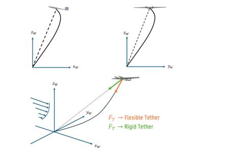
Figure 1: Visualization of tether sag and its effect on the aircraft.

Different studies have been conducted to develop more accurate models for tethers. Du et al. extract the equation of a variable length cable using an absolute nodal coordinate formulation and then discretize the cable by means of a finite number of elements to decrease the computational cost [13]. Similarly, [14] utilizes the same approach to model the cable, and solves the whole AWES, including aircraft, tether and aircraft, by a variational integrator to increase the performance. In another approach, the tether is considered to correspond to a fixed number of lumped masses connected by spring-damper elements to generate a coherent model [15, 16]. Although modeling the tether with the above-mentioned methods increases the accuracy, they add three degrees of freedom for each rod/lumped mass, increasing the whole system’s number of dimensions drastically. To tackle this difficulty, [12] introduced a quasi-static approach, in which the elastic vibrations are neglected and the cable tension and shape are assumed to be the results of mass and drag. Notwithstanding that the simulation of small-scale AWESs with a quasi-static approach for the tether has been verified with flight tests [17], there is only one study available that makes use of a model of a flexible tether for the path planning [18]. In that study only the landing of a simple aircraft in 2D is examined.

The contribution of this paper is found in the establishment of an optimal path planning framework for a 6-DOF aircraft, winch, and flexible tether AWES during both the traction and retraction phases. From a numerical optimization standpoint, we introduce an index-1 DAE formulation for AWES and a minimal coordinate representation, which eliminates consistency condition problems and drift arising from index reduction of higher index DAE formulations. To solve the resulting trajectory optimization problem, we introduce direct multiple shooting in the penalty-based homotopy approach [6]. The paper is structured as follows, in Section II we describe the AWES model which builds on the MegAWES toolbox [19]. Subsequently, the optimization method and its implementation using CasADi [20] are discussed in Section III. Finally, in Secretion IV, the simulation results are presented to show the effectiveness of the proposed optimization method for AWESs with the flexible tether.

II Modeling

Our modeling approach follows the methodology established by MegAWES [19]. The model distinguishes itself from those used by other optimization tools, such as AWEBOX [6], in two critical aspects. First a minimal coordinate representation is used to parameterize the aircraft’s attitude instead of an element of $\mathfrak{SO}(3)$. This is strictly a modeling choice. Second a flexible tether model is included instead of a rigid tether model. A flexible tether increases the physical accurateness of the resulting model. Both of these model features have a positive effect on the subsequent optimization. This will be discussed in more detail in the next section.

II-A Parameterization and kinematics

Consider two frames of reference $\mathcal{O}$ and $\mathcal{B}$. Reference frame $\mathcal{O}$ is used as an inertial frame of reference whereas frame $\mathcal{B}$ is attached to the aircraft. Therefore the attitude of the aircraft can be represented as the rotation matrix, $\mathrm{R}_{\mathcal{O}}^{\mathcal{B}}\in\mathfrak{SO}(3)$, that maps $\mathcal{O}$ into $\mathcal{B}$. As is standard in the aerospace community, we use the Euler angles to parameterize the attitude. The angles are gathered in a coordinate vector, $\bm{\mathbf{q}}_{\text{a}}\in\mathbb{R}^{3}$.

$$\mathrm{R}_{\mathcal{O}}^{\mathcal{B}}=\mathrm{R}_{x}(\phi)\mathrm{R}_{y}(\theta)\mathrm{R}_{z}(\psi)$$ (1)

The time derivative of the coordinate vector, $\bm{\mathbf{q}}_{\text{a}}$, is related to the angular velocity of the aircraft by a geometric Jacobian.

$$\bm{\mathbf{\omega}}_{\text{aircraft}}^{\mathcal{B}}=\begin{pmatrix}c_{\theta}c_{\psi}&s_{\psi}&0\\ -s_{\psi}&c_{\psi}&0\\ s_{\theta}c_{\psi}&0&1\end{pmatrix}\dot{\bm{\mathbf{q}}}_{\text{a}}$$ (2)

where $c_{(.)}$ and $s_{(.)}$ denote $\cos{(.)}$ and $\sin{(.)}$, respectively.

We introduce a third frame of reference $\mathcal{W}$ whose $x$-axis aligns with the wind direction at an angle $\zeta$ from the inertial $x$-axis and whose $z$-axis points upward, opposite to the downward direction of the inertial $z$-axis.

$$\mathrm{R}_{\mathcal{O}}^{\mathcal{W}}=\mathrm{R}_{z}(\zeta)\mathrm{R}_{x}(\pi)$$ (3)

The position of the aircraft is parameterized using spherical coordinates, $\bm{\mathbf{q}}_{\text{s}}\in\mathbb{R}^{3}$, where the first and second elements of $\bm{\mathbf{q}}_{\text{s}}$ are azimuth and polar angles, as shown in Fig. 2, and the third one denotes the radial distance from the origin to the aircraft. To that end, we introduce a forth and final frame of reference $\mathcal{T}$ whose motion relative to $\mathcal{W}$ is parameterized by the azimuth, $\lambda$, and polar, $\eta$, angles and so that the local $z$-axis is pointing away from the aircraft to the origin. In local coordinates the position of the aircraft is then characterized by the distance $r$ along the $z$-direction.

$$\mathrm{R}_{\mathcal{W}}^{\mathcal{T}}=\mathrm{R}_{z}(\lambda)\mathrm{R}_{y}(-\eta)\mathrm{R}_{y}(-\tfrac{\pi}{2})$$ (4)

The time derivative of the coordinate vector, $\bm{\mathbf{q}}_{\text{s}}$, is related to the linear velocity of the aircraft by another geometric Jacobian.

$$\bm{\mathbf{v}}_{\text{aircraft}}^{\mathcal{W}}=\begin{pmatrix}c_{\lambda}c_{\eta}&-s_{\lambda}c_{\eta}r&-c_{\lambda}s_{\eta}r\\ s_{\lambda}c_{\eta}&c_{\lambda}c_{\eta}r&-s_{\lambda}s_{\eta}r\\ s_{\eta}&0&c_{\eta}r\end{pmatrix}\dot{\bm{\mathbf{q}}}_{\text{s}}$$ (5)

A visualization of the frames is presented in Fig. 2.

II-B Wind and atmosphere model

Since AWESs typically operate at an altitude of several hundred meters, it is common practice among the research community to model a horizontal atmospheric wind shear to estimate the mean wind speed more accurately. In this manuscript, the wind speed as a function of the height, $z$, is determined using a logarithmic wind profile

$$\bm{\mathbf{v}}_{\text{wind}}^{\mathcal{W}}=v_{\text{ground}}\frac{\log z/z_{0}}{\log z_{\text{ref}}/z}\bm{\mathbf{E}}_{1}^{\mathcal{W}}$$ (6)

where $v_{\text{ground}}$ is the measured ground wind speed at height $z_{\text{ref}}$, $z_{0}$ is referred to as the roughness length, and $\bm{\mathbf{E}}_{1}^{\mathcal{W}}$ denotes th first component of the unit vector in the wind reference frame.

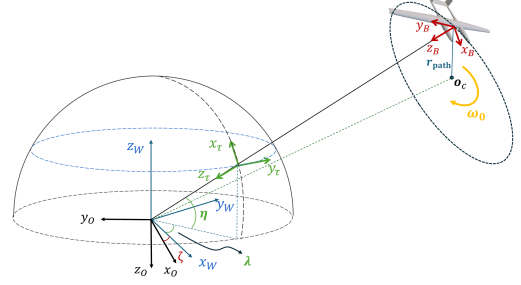
Figure 2: Visualization of initial circular path concept, and the reference frames ($\mathcal{O}$ (black), $\mathcal{W}$ (blue), $\mathcal{\tau}$ (green), $\mathcal{B}$ (red)).

II-C Rigid-body aircraft dynamics

The rigid body dynamics of an aircraft are described in numerous references, such as [21]. The main difference between modeling an ordinary aircraft and a tethered one, is the tether force. In this context, we assume that the tether force acts on the aircraft’s center of gravity. This means that no torque is applied to the aircraft due to the tether. The aircraft’s dynamics are governed by

$$m\dot{\bm{\mathbf{v}}}_{\text{aircraft}}^{\mathcal{B}}+m\bm{\mathbf{\omega}}_{\text{aircraft}}^{\mathcal{B}}\times\bm{\mathbf{v}}_{\text{aircraft}}^{\mathcal{B}} =\bm{\mathbf{f}}_{\text{aircraft}}^{\mathcal{B}}$$ (7a)

$$\mathrm{J}\dot{\bm{\mathbf{\omega}}}_{\text{aircraft}}^{\mathcal{B}}+\bm{\mathbf{\omega}}_{\text{aircraft}}^{\mathcal{B}}\times\mathrm{J}\bm{\mathbf{\omega}}_{\text{aircraft}}^{\mathcal{B}} =\bm{\mathbf{\tau}}_{\text{aircraft}}^{\mathcal{B}}$$ (7b)

where $\bm{\mathbf{v}}_{\text{aircraft}}^{\mathcal{B}}$ is the aircraft velocity in the body reference frame, $\bm{\mathbf{\omega}}_{\text{aircraft}}^{\mathcal{B}}$ is the angular velocity vector between body and inertial reference frames. $m$ and $\mathrm{J}$ represent the aircraft mass and inertia, respectively.

The total force, $\bm{\mathbf{f}}_{\text{aircraft}}$, includes aerodynamic, tether, and gravitational forces. The total torque, $\bm{\mathbf{\tau}}_{\text{aircraft}}$, includes only aerodynamics torques.

$$\bm{\mathbf{f}}_{\text{aircraft}}^{\mathcal{B}} =\bm{\mathbf{f}}_{\text{aircraft,aero}}^{\mathcal{B}}+\bm{\mathbf{f}}_{\text{aircraft,tether}}^{\mathcal{B}}+\mathrm{R}_{\mathcal{O}}^{\mathcal{B}}(mg\bm{\mathbf{E}}_{3}^{\mathcal{O}})$$ (8a)

$$\bm{\mathbf{\tau}}_{\text{aircraft}}^{\mathcal{B}} =\bm{\mathbf{\tau}}_{\text{aircraft,aero}}^{\mathcal{B}}$$ (8b)

II-D Aerodynamic model

In this work, we adopt the MegAWES aerodynamic model [19]. MegAWES utilizes pre-calculated static aerodynamic coefficients stored in lookup tables to compute the aerodynamic forces and torques acting on the wing, elevator, and rudder, independently as a function of the aircraft’s apparent velocity (9a), angle of attack (9b), side slip angle (9c), and deflections of control surfaces.

$$\bm{\mathbf{v}}_{a} =\bm{\mathbf{v}}_{\text{aircraft}}^{\mathcal{W}}-\bm{\mathbf{v}}_{\text{wind}}^{\mathcal{W}}$$ (9a)

$$\alpha =-\arctan\frac{v_{\text{aircraft,z}}^{\mathcal{B}}-v_{\text{wind,z}}^{\mathcal{B}}}{v_{\text{aircraft,x}}^{\mathcal{B}}-v_{\text{wind,x}}^{\mathcal{B}}}$$ (9b)

$$\beta =\arctan\frac{v_{\text{aircraft,y}}^{\mathcal{B}}-v_{\text{wind,y}}^{\mathcal{B}}}{v_{\text{aircraft,x}}^{\mathcal{B}}-v_{\text{wind,x}}^{\mathcal{B}}}$$ (9c)

To retain a differentiable model, here we have replaced the look-up tables with second-order polynomials of the following form

$$\mathcal{C}_{i}(\alpha) =\mathcal{C}_{i,2}\alpha^{2}+\mathcal{C}_{i,1}\alpha+\mathcal{C}_{i,0}$$ (10)

where the index $i\in\{L,D,M\}$ determines the coefficients of lift and drag forces and the pitch moment of the wing. Similarly, for the rudder and elevator, $i\in\{L,D\}$ specifies the lift and drag forces. Additional information can be found in [19].

II-E Winch model

AWESs with a fixed ground station consist of a winch and a generator. We consider a simple 1-DOF winch model. This is similar to [22].

$$J_{\text{winch}}\ddot{\theta}_{\text{winch}}+b_{\text{winch}}\dot{\theta}_{\text{winch}}=r_{\text{winch}}\|\bm{\mathbf{f}}_{\text{winch,tether}}\|-\tau_{\text{generator}}$$ (11)

where $\dot{\theta}_{\text{winch}}$, $J_{\text{winch}}$, $r_{\text{winch}}$, and $b_{\text{winch}}$ represent the winch’s angular velocity, inertia, radius, and viscous friction, respectively. The amplitude, $\|\bm{\mathbf{f}}_{\text{winch,tether}}\|\neq 0$ is equal to the tether force magnitude evaluated at the winch. Finally we have the the motor/generator torque, $\tau_{\text{generator}}$, which will be treated as a control input.

II-F Quasi-static flexible tether model

Other references simplify the physics of the tether in an effort to ease its later treatment by the optimizer [5, 6, 7]. This comes at the cost of a loss of physical accurateness which, as we will demonstrate, can severely impact the optimization result. The goal of this work is to incorporate a tether model in the optimization pipeline that strikes a better balance between physical accurateness yet manageable numerical treatment.

To that end we adopt the quasi-static modeling approach from [12]. It can account for tether sag as well as elastic tether deformation. The model is incapable of capturing any dynamic modes of the tether, yet it results in a physically accurate and computationally efficient model that approximates the tether by a number of discrete lumped masses connected with massless elastic (or inelastic) segments. The primary assumption is that the tether remains in a state of quasi-static equilibrium. This means that all the forces acting on each of the lumped masses - which include, gravitational, drag and constraint forces, agree with the prescribed motion of the tether. Further details are provided below.

First note that the tether length is a dynamic variable that is related to the other system variables. Specifically we have that

$$l=r_{\text{winch}}\theta_{\text{winch}}$$ (12)

Second we approximate the cable with a total of $N$ lumped masses. We describe every mass, $j$, with its position which is denoted with the vector $\bm{\mathbf{p}}_{j}$. Indexing is done such that $\bm{\mathbf{p}}_{0}$ coincides with the aircraft and $\bm{\mathbf{p}}_{N+1}$ with the winch. The nominal length and mass of each cable segment are defined as

$$L_{s} =\tfrac{1}{N+1}l$$ (13a)

$$m_{j} =\rho_{\text{tether}}L_{s}$$ (13b)

where $\rho_{\text{tether}}$ represents the cable’s mass density.

The principle idea behind the model is to construct a recursive calculation that runs over all masses in the discretized cable model and determines their position and associated constraint forces. The model takes as inputs the tether force at the winch and outputs the corresponding position of the final mass. The recursion thus is initialized with $j=N+1$ and ends with $j=0$. The latter should coincide with the position of the aircraft. When the position of the aircraft is known, a root finding problem can be established to determine the associated tether force.

To determine the calculation procedure, we can consider the equation of motion of the $j$^th mass. To simplify notation the superscript is left out in this section and all vectors are expressed in the wind frame of reference

$$m_{j}\ddot{\bm{\mathbf{p}}}_{j}=\bm{\mathbf{f}}_{j-1}-\bm{\mathbf{f}}_{j}+\bm{\mathbf{f}}_{j,\text{drag}}-m_{j}g\bm{\mathbf{E}}_{3}$$ (14)

where $\bm{\mathbf{f}}_{j}$ denotes the constraint force shared with the preceding mass, $\bm{\mathbf{f}}_{j-1}$ denotes the constraint force shared with the following mass, $\bm{\mathbf{f}}_{j,\text{drag}}$ denoted the local drag force and the final term represents gravitational effects. We can now further specify all elements from the equation. The recursion will follow.

First it is assumed that the velocity of each mass along the cable is computed as the sum of the radial velocity induced by the aircraft and the angular rotation of the segment and the the acceleration of each segment is computed from the centrifugal component only. In other words, the tether behaves as a rigid body every time instant.

$$\dot{\bm{\mathbf{p}}}_{j} =\bm{\mathbf{v}}_{\text{tether}}+\bm{\mathbf{\omega}}_{\text{tether}}\times\bm{\mathbf{p}}_{j}$$ (15a)

$$\ddot{\bm{\mathbf{p}}}_{j} =\bm{\mathbf{\omega}}_{\text{tether}}\times(\bm{\mathbf{\omega}}_{\text{tether}}\times\bm{\mathbf{p}}_{j})$$ (15b)

The radial velocity and angular rotation of the aircraft are defined as

$$\bm{\mathbf{v}}_{\text{tether}} =\tfrac{1}{\|\bm{\mathbf{p}}_{\text{aircraft}}\|^{2}}\left\langle\bm{\mathbf{p}}_{\text{aircraft}},\bm{\mathbf{v}}_{\text{aircraft}}\right\rangle\bm{\mathbf{p}}_{\text{aircraft}}$$ (16a)

$$\bm{\mathbf{\omega}}_{\text{tether}} =\tfrac{1}{\|\bm{\mathbf{p}}_{\text{aircraft}}\|^{2}}\bm{\mathbf{p}}_{\text{aircraft}}\times\bm{\mathbf{v}}_{\text{aircraft}}$$ (16b)

The drag force acting on the $j$^th mass is defined as

$$\bm{\mathbf{f}}_{j,\text{drag}}=-\frac{1}{2}\rho d_{\text{tether}}L_{j}C_{D}\|\bm{\mathbf{v}}_{j,\perp}\|\bm{\mathbf{v}}_{j,\perp}$$ (17)

where $d_{\text{tether}}$ represents the tether diameter, $\rho$ is the air density at the $j$^th segment and is calculated similar to (6), $C_{D}$ is the normal drag coefficient and $\bm{\mathbf{v}}_{j,\perp}$ is the normal component of relative wind velocity at each segment. The normal $\bm{\mathbf{v}}_{j,\perp}$ and parallel $\bm{\mathbf{v}}_{j,\parallel}$ components of each segment can be calculated as

$$\bm{\mathbf{v}}_{j,\perp} =\bm{\mathbf{v}}_{j}-\bm{\mathbf{v}}_{j,\parallel}$$ (18a)

$$\bm{\mathbf{v}}_{j,\parallel} =\tfrac{1}{\|\Delta\bm{\mathbf{p}}_{j}\|^{2}}\left\langle\Delta\bm{\mathbf{p}}_{j},\bm{\mathbf{v}}_{j}\right\rangle\Delta\bm{\mathbf{p}}_{j}$$ (18b)

where $\Delta\bm{\mathbf{p}}_{j}=\bm{\mathbf{p}}_{j-1}-\bm{\mathbf{p}}_{j}$, and relative wind velocity at each segment reads as

$$\bm{\mathbf{v}}_{j}=\dot{\bm{\mathbf{p}}}_{j}-\bm{\mathbf{v}}_{j,\text{wind}}=\dot{\bm{\mathbf{p}}}_{j}-\bm{\mathbf{v}}_{\text{wind}}(z_{j})$$ (19)

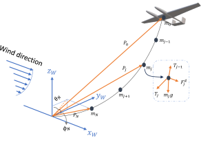
Figure 3: Visualization of tether lumped masses and forces in the wind frame.

Now provided that $\bm{\mathbf{f}}_{j}$ and $\bm{\mathbf{p}}_{j}$ are known, equation (14) can be manipulated to yield $\bm{\mathbf{f}}_{j-1}$. Once $\bm{\mathbf{f}}_{j-1}$ is known, the position of the $j$^th mass can be calculated. According to the Hook’s law we have that

$$l_{j-1}=L_{s}\left(1+\frac{\|\bm{\mathbf{f}}_{j-1}\|}{E_{\text{tether}}A_{\text{tether}}}\right)$$ (20)

where $E_{\text{tether}}$ and $A_{\text{tether}}$ are tether Young’s modulus and cross-section area. Due to the assumption that the tether is in static equilibrium it also follows that

$$\bm{\mathbf{p}}_{j-1}=\bm{\mathbf{p}}_{j}+l_{j-1}\frac{\bm{\mathbf{f}}_{j-1}}{\|\bm{\mathbf{f}}_{j-1}\|}$$ (21)

These equations thus produce the anticipated recursion. We can parameterize the first constraint force and solve for $\bm{\mathbf{p}}_{0}$. By definition we find the following algebraic equation

$$\bm{\mathbf{p}}_{\text{aircraft}}^{\mathcal{W}}-\bm{\mathbf{p}}_{0}=0$$ (22)

Solving for the roots of this equation as a function of the first constraint force determine the quasi-static model. The force acting on the aircraft is evaluated as

$$\bm{\mathbf{f}}_{\text{aircraft},\text{tether}}^{\mathcal{B}}=-\mathrm{R}_{\mathcal{O}}^{\mathcal{B}}\mathrm{R}_{\mathcal{W}}^{\mathcal{O}}\bm{\mathbf{f}}_{0}$$ (23)

In this work we parameterize the first constraint force as follows

$$\bm{\mathbf{f}}_{N} =T\begin{pmatrix}s_{\theta_{N}}c_{\phi_{N}}&s_{\phi_{N}}&c_{\theta_{N}}c_{\phi_{N}}\end{pmatrix}^{\top}$$ (24a)

$$\bm{\mathbf{p}}_{N} =L_{s}\begin{pmatrix}s_{\theta_{N}}c_{\phi_{N}}&s_{\phi_{N}}&c_{\theta_{N}}c_{\phi_{N}}\end{pmatrix}^{\top}$$ (24b)

Here $T$, $\theta_{N}$ and $\phi_{N}$ denote the magnitude of the force and the spherical angles that determine the direction of force to the nearest point mass to the winch, as depicted in Fig. 3.

III Optimization

The goal of this work is now to integrate the model from the previous section in an optimization framework tailored to generating periodic flight trajectories maximizing power generation. This means that we are looking for feasible trajectories that can be repeated infinitely and convert the maximum amount of wind energy into electrical energy with every cycle.

This problem formulation results into a challenging optimal control problem that requires careful numerical treatment. Our approach draws much inspiration from AWEBOX [6] but instead uses a minimal coordinate representation of the attitude and the flexible tether model. The use of the quasi-static flexible tether model furthermore introduces some additional challenges that require further treatment.

III-A Problem formulation

We aim to generate periodic maximum power flight trajectories for AWES system. Similar to other work, therefore we propose to solve the following periodic continuous-time Optimal Control Problem (OCP).

$$\min_{\bm{\mathbf{w}}}\frac{1}{T}\int_{t=0}^{T}c(\bm{\mathbf{x}}(t),\bm{\mathbf{u}}(t),\bm{\mathbf{z}}(t))\text{d}t$$ (25)

$$\begin{aligned} \text{s.t. }0&=\bm{\mathbf{F}}(\dot{\bm{\mathbf{x}}}(t),\bm{\mathbf{x}}(t),\bm{\mathbf{u}}(t),\bm{\mathbf{z}}(t)),\forall t\in[0,T)\\ 0&\geq\bm{\mathbf{H}}(\bm{\mathbf{x}}(t),\bm{\mathbf{u}}(t),\bm{\mathbf{z}}(t)),\forall t\in[0,T)\\ 0&=\bm{\mathbf{x}}(0)-\bm{\mathbf{x}}(T)\\ 0&=\Psi(\bm{\mathbf{x}}(0))\end{aligned}$$

The OCP is fully specified by definition of the cost rate function, $c$, the differential and possibly other equality constraints, $\bm{\mathbf{F}}$, and the inequality path constraints $\bm{\mathbf{H}}$.

In this subsection, we define all components in (25) for the considered AWES. In the next subsections we detail our solution strategy which has been tailored to the specific requirements posed by this problem.

Variables

The differential states, $\bm{\mathbf{x}}$, control inputs, $\bm{\mathbf{u}}$, and algebraic states, $\bm{\mathbf{z}}$, are defined as

$$\bm{\mathbf{x}} =\begin{pmatrix}\theta_{\text{winch}}&\dot{\theta}_{\text{winch}}&\bm{\mathbf{v}}_{\text{aircraft}}^{\mathcal{B},\top}&\bm{\mathbf{\omega}}_{\text{aircraft}}^{\mathcal{B},\top}&\bm{\mathbf{q}}_{\text{a}}^{\top}&\bm{\mathbf{q}}_{\text{s}^{\top}}\end{pmatrix}^{\top}$$ (26a)

$$\bm{\mathbf{z}} =\begin{pmatrix}T&\theta_{N}&\phi_{N}\end{pmatrix}^{\top}$$ (26b)

$$\bm{\mathbf{u}} =\begin{pmatrix}\tau_{\text{generator}}&\delta_{\text{aileron}}&\delta_{\text{elevator}}&\delta_{\text{rudder}}\end{pmatrix}^{\top}$$ (26c)

The concatenation of all variables is denoted $\bm{\mathbf{w}}=\begin{pmatrix}\bm{\mathbf{x}}^{\top}&\bm{\mathbf{u}}^{\top}&\bm{\mathbf{z}}^{\top}\end{pmatrix}^{\top}$

Dynamics

The OCP in (25) makes use of a general form of DAEs defined in fully implicit form, $\bm{\mathbf{F}}$. In this work a semi-explicit DAE description of the system dynamics is available so that we can further specify the DAE as

$$\bm{\mathbf{F}}={\begin{pmatrix}\bm{\mathbf{\dot{x}}}-\bm{\mathbf{f}}(\bm{\mathbf{x}}(t),\bm{\mathbf{u}}(t),\bm{\mathbf{z}}(t))\\ \bm{\mathbf{g}}(\bm{\mathbf{x}}(t),\bm{\mathbf{z}}(t))\end{pmatrix}}=0$$ (27)

Here the algebraic, $\bm{\mathbf{g}}$, and, differential, $\bm{\mathbf{f}}$, equations corresponded to the tether dynamics (22) and the concatenation of the winch (11) and aircraft dynamics (2, 5, 7), respectively.

Cost

Similar to other studies such as [5, 6], the cost function in (25) can be expressed as the sum of negative power output and a penalty on the angular velocity rate of the aircraft and side slip angle to maximize the power output whilst also avoiding aggressive maneuvers.

$$c(\bm{\mathbf{x}},\bm{\mathbf{u}},\bm{\mathbf{z}})=-P+\|\bm{\mathbf{\xi}}\|_{\Gamma}^{2}$$ (28)

Here $P=\dot{\theta}_{\text{winch}}\tau_{\text{generator}}$, $\bm{\mathbf{\xi}}=\begin{pmatrix}\dot{\bm{\mathbf{\omega}}}_{\text{aircraft}}^{\mathcal{B}}&\beta\end{pmatrix}^{\text{T}}$, and $\Gamma$ is a constant diagonal weight matrix.

Path constraints

The inequality constraints or path constraints, $\bm{\mathbf{H}}$, include the limitations related to the tether force (29a), flight region (29b,29c), winch acceleration (29d), and aerodynamics (29e-29i) of the AWES can be summarized as follows

$$\underline{f} \leq\|\bm{\mathbf{f}}_{\text{aircraft,tether}}\|\leq\overline{f}$$ (29a)

$$\underline{y} \leq y^{\mathcal{O}}_{\text{aircraft}}\leq\overline{y}$$ (29b)

$$\underline{z} \leq z^{\mathcal{O}}_{\text{aircraft}}\leq\overline{z}$$ (29c)

$$\underline{\ddot{\theta}}_{\text{winch}} \leq{\ddot{\theta}}_{\text{winch}}\leq\overline{\ddot{\theta}}_{\text{winch}}$$ (29d)

$$\underline{\bm{\mathbf{v}}}_{\text{a}} \leq\|\bm{\mathbf{v}}_{\text{a}}\|\leq\overline{\bm{\mathbf{v}}}_{\text{a}}$$ (29e)

$$\underline{\alpha} \leq\alpha\leq\overline{\alpha}$$ (29f)

$$\underline{\beta} \leq\beta\leq\overline{\beta}$$ (29g)

$$\underline{\alpha}_{\text{elevator}} \leq\alpha+\alpha_{\text{elevator,damped}}+\delta_{\text{elevator}}\leq\overline{\alpha}_{\text{elevator}}$$ (29h)

$$\underline{\beta}_{\text{rudder}} \leq\beta+\beta_{\text{rudder,damped}}+\delta_{\text{rudder}}\leq\overline{\beta}_{\text{rudder}}$$ (29i)

$$\underline{\delta}_{\text{aileron}} \leq\delta_{\text{aileron,damped}}+{\delta}_{\text{aileron}}\leq\overline{\delta}_{\text{aileron}}$$ (29j)

where $\|\bm{\mathbf{v}}_{\text{a}}\|$ denotes the apparent velocity magnitude, $\alpha_{\text{elevator,damped}}$ (29h), $\beta_{\text{rudder,damped}}$ (29i), and $\delta_{\text{aileron,damped}}$ (29j) represent the corrected aerodynamic angles for different control surfaces [19].

Furthermore, the tether and aircraft must not collide. Accordingly, the angle between $\bm{\mathbf{f}}_{\text{tether}}^{\mathcal{B}}$ and the $xy$-plane in the body reference frame is restricted to avoid any contact between tether and aircraft where the angles describing the tether force in the body reference frame are chosen as shown in Fig. 4.

$$\underline{\theta_{T}}\leq\theta_{T}\leq\overline{\theta_{T}}$$ (30)

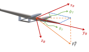
Figure 4: The constraint on tether angle to avoid collision.

An optional constraint can be implemented to enforce the winch velocity to remain positive during the traction phase, thereby enhancing the quality of the optimal path and reducing computational effort. This requirement dictates that the power for the traction phase must remain positive for a specific duration within the simulation (since the traction force is supposed to be positive).

$$\dot{\theta}_{\text{winch}}>0,\;\forall t\leq c_{\text{ro}}T,\;c_{\text{ro}}\in\begin{pmatrix}0&1\end{pmatrix}$$ (31)

Obviously, choosing a high value for $c_{\text{ro}}$ makes the problem infeasible.

Initial value constraint

Finally, the initial value constraint is embedded in function $\Psi$, where $\Psi(\bm{\mathbf{x}})=0$, is used to enforce consistency conditions for higher-order DAEs. Here, it can be utilized for the cold start of the tether dynamics and for defining other constraints that can enhance the performance of the optimal path or might assist the system operation in take-off or landing. These aspects are further addressed in the simulation and results section.

III-B Discretization

Problem (25) cannot be solved analytically. The problem is transcribed into a nonlinear program (NLP) that we can treat numerically instead with Sequential Quadratic Programming (SQP) and Interior Point (IP) methods. To that end we make use of the Direct Multiple Shooting (DMS) technique.

To transform the OCP into an NLP through DMS, the control and state variables are discretized over a time grid, dividing the time interval into smaller sub-intervals, or shooting intervals. We formally introduce time instants $\{t_{n}\}$ so that $0=t_{0}<\dots<t_{n}<\dots t_{N}=T$. For every time instant we introduce an optimization variable, $\bm{\mathbf{w}}_{n}=\bm{\mathbf{w}}(t_{n})$. We overwrite notation an refer to the concatenation of all optimization variables $\{\bm{\mathbf{w}}_{n}\}$ as $\bm{\mathbf{w}}$.

For the given states and controls in each shooting interval, the equality constraints (27) are discretized using a backward implicit Euler method, as shown in (32), ensuring the equations of motion remain valid over time. The backward Euler method is chosen here for the sake of simplicity. Furthermore, by choosing a sufficient number of shooting nodes, the numerical errors remain small. Note that our approach does not exclude the use of more advanced integration techniques.

$$0 =\bm{\mathbf{x}}_{{n+1}}-\bm{\mathbf{x}}_{n}-\Delta t\bm{\mathbf{f}}(\bm{\mathbf{x}}_{{n+1}},\bm{\mathbf{u}}_{n},\bm{\mathbf{z}}_{{n+1}})$$ (32a)

$$0 =\bm{\mathbf{g}}(\bm{\mathbf{x}}_{{n+1}},\bm{\mathbf{z}}_{{n+1}})$$ (32b)

Similarly, the cost function is approximated by numerical quadrature.

$$\int_{0}^{T}c(\bm{\mathbf{x}}(t),\bm{\mathbf{u}}(t),\bm{\mathbf{z}}(t))\text{d}t=\sum_{n=0}^{N-1}\Delta tc(\bm{\mathbf{x}}_{{n+1}},\bm{\mathbf{u}}_{n},\bm{\mathbf{z}}_{{n+1}})$$ (33)

Finally, the NLP acquired by discretization of the OCP is solved with the IPOPT solver [23] in combination with the MUMPS linear solver [24] alongside with CasADi [20] for algorithmic differentiation.

III-C Homotopy strategy

The DAE, $\bm{\mathbf{F}}$, spans a constraint manifold that contains all trajectories that can be achieved with the present system. The goal of the optimizer is to navigate this set and find a feasible trajectory that is also optimal. For strongly under-actuated and highly non-linear dynamics this manifold can be very complex and finding elements in this set becomes increasingly difficult, let alone navigate it in pursuit of the optimal feasible behavior. This may cause the optimization algorithm to converge prematurely or fail altogether.

To ease the challenges faced by the optimization algorithm, homotopy approaches can be used. Their purpose is to decrease the overall computational cost and improve the solver’s reliability and robustness [25, 6, 26, 27]. Within a homotopy, challenging optimization problems are treated by solving a sequence of easier, manageable problems that gradually transition to the original, complex problem. To that end the OCP in (25) is reformulated as

$$\min_{\tilde{\bm{\mathbf{w}}},\bm{\mathbf{\Phi}}}\frac{1}{T}\int_{t=0}^{T}c_{\Phi}(\bm{\mathbf{x}}(t),\tilde{\bm{\mathbf{u}}},\bm{\mathbf{z}}(t),\bm{\mathbf{\Phi}})+\bm{\mathbf{s}}^{\top}\bm{\mathbf{\Phi}}\;\text{d}t$$ (34)

$$\begin{aligned} \text{s.t. }0&=\bm{\mathbf{F}}_{\Phi}(\dot{\bm{\mathbf{x}}}(t),\bm{\mathbf{x}}(t),\tilde{\bm{\mathbf{u}}}(t),\bm{\mathbf{z}}(t),\bm{\mathbf{\Phi}}),\leavevmode\nobreak\ \forall t\in[0,T)\\ 0&\geq\bm{\mathbf{H}}(\bm{\mathbf{x}}(t),\tilde{\bm{\mathbf{u}}}(t),\bm{\mathbf{z}}(t)),\leavevmode\nobreak\ \forall t\in[0,T)\\ 0&=\bm{\mathbf{x}}(0)-\bm{\mathbf{x}}(T)\\ 0&=\Psi(\bm{\mathbf{x}}(0))\end{aligned}$$

where $\bm{\mathbf{\Phi}}\in(\underline{\bm{\mathbf{\Phi}}},\overline{\bm{\mathbf{\Phi}}})$ are bounded decision variables (homotopy parameters) that can be used to gradually increase the complexity of the problem, and $\bm{\mathbf{s}}\in\mathbb{R}_{+}^{n_{\Phi}}$ are positive penalty variables. The differential and algebraic variables are equivalent to those in problem (25) but we note that the input variables are updated as

$$\tilde{\bm{\mathbf{u}}} =\begin{pmatrix}\bm{\mathbf{u}}^{\top}&\hat{\bm{\mathbf{u}}}^{\top}\end{pmatrix}^{\top}$$ (35a)

$$\hat{\bm{\mathbf{u}}} =\begin{pmatrix}\bm{\mathbf{f}}_{\text{fict}}^{\mathcal{B},\top}&\bm{\mathbf{\tau}}_{\text{fict}}^{\mathcal{B},\top}&{f}_{\text{aircraft,prop}}^{\mathcal{B}}\end{pmatrix}^{\top}$$ (35b)

Here $\bm{\mathbf{f}}_{\text{fict}}^{\mathcal{B}}$ and $\bm{\mathbf{\tau}}_{\text{fict}}^{\mathcal{B}}$ are fictitious forces and torques that are used in early homotopy stages and that are assumed to act directly on the aircraft body instead of the aerodynamic force and torques. A non-physical propulsion/brake force $\bm{\mathbf{f}}_{\text{aircraft,prop}}^{\mathcal{B}}$ is also applied in $x$-axis of body reference frame. Accordingly, the optimization parameters in (34) are defined as $\tilde{\bm{\mathbf{w}}}=\begin{pmatrix}\bm{\mathbf{x}}^{\top}&\tilde{\bm{\mathbf{u}}}^{\top}&\bm{\mathbf{z}}^{\top}\end{pmatrix}^{\top}$.

For this study, three homotopy stages are used ($n_{\Phi}=3$). In the first homotopy step, fictitious forces and torques are gradually removed from the initial solver, restoring the original aerodynamics. This transition is facilitated by relying on the propulsion/braking force. In the second stage, the propulsion or braking force is set to zero. The DAE $\bm{\mathbf{F}}_{\Phi}$ in (34) is thus similar with $\bm{\mathbf{F}}$, except that the aerodynamic forces applied to the aircraft in (8) are replaced by

$$\begin{multlined}\begin{pmatrix}{\bm{\mathbf{f}}}_{\text{aircraft}}^{\mathcal{B}}\\ {\bm{\mathbf{\tau}}}_{\text{aircraft}}^{\mathcal{B}}\end{pmatrix}\leftarrow(1-\Phi_{1})\begin{pmatrix}{\bm{\mathbf{f}}}_{\text{aircraft},\text{aero}}^{\mathcal{B}}\\ {\bm{\mathbf{\tau}}}_{\text{aircraft},\text{aero}}^{\mathcal{B}}\end{pmatrix}\\ +\Phi_{1}\begin{pmatrix}\bm{\mathbf{f}}_{\text{fict}}^{\mathcal{B}}\\ \bm{\mathbf{\tau}}_{\text{fict}}^{\mathcal{B}}\end{pmatrix}+\Phi_{2}\;{f}_{\text{aircraft,prop}}^{\mathcal{B}}\bm{\mathbf{E}}_{x}^{\mathcal{B}}\end{multlined}\begin{pmatrix}{\bm{\mathbf{f}}}_{\text{aircraft}}^{\mathcal{B}}\\ {\bm{\mathbf{\tau}}}_{\text{aircraft}}^{\mathcal{B}}\end{pmatrix}\leftarrow(1-\Phi_{1})\begin{pmatrix}{\bm{\mathbf{f}}}_{\text{aircraft},\text{aero}}^{\mathcal{B}}\\ {\bm{\mathbf{\tau}}}_{\text{aircraft},\text{aero}}^{\mathcal{B}}\end{pmatrix}\\ +\Phi_{1}\begin{pmatrix}\bm{\mathbf{f}}_{\text{fict}}^{\mathcal{B}}\\ \bm{\mathbf{\tau}}_{\text{fict}}^{\mathcal{B}}\end{pmatrix}+\Phi_{2}\;{f}_{\text{aircraft,prop}}^{\mathcal{B}}\bm{\mathbf{E}}_{x}^{\mathcal{B}}$$ (36)

To expedite solving the OCP with the most accurate model, the cost function is initially designed to minimize aircraft angular acceleration and side slip, keeping the aircraft close to its initial path by the end of the second homotopy stage. In the final homotopy stage, the cost function shifts its focus to the power harvesting mode. The cost function $c_{\phi}$ is defined as

$$\begin{multlined}c_{\phi}(\bm{\mathbf{x}}(t),\bm{\mathbf{u}}(t),\bm{\mathbf{z}}(t),\bm{\mathbf{\phi}})=\\ -(1-\Phi_{3})P+\|\bm{\mathbf{\xi}}\|_{\Gamma}^{2}+\Phi_{3}\|\bm{\mathbf{x}}(t)-\bm{\mathbf{x}}_{0}(t)\|_{\Lambda}^{2}\end{multlined}c_{\phi}(\bm{\mathbf{x}}(t),\bm{\mathbf{u}}(t),\bm{\mathbf{z}}(t),\bm{\mathbf{\phi}})=\\ -(1-\Phi_{3})P+\|\bm{\mathbf{\xi}}\|_{\Gamma}^{2}+\Phi_{3}\|\bm{\mathbf{x}}(t)-\bm{\mathbf{x}}_{0}(t)\|_{\Lambda}^{2}$$ (37)

where $\Gamma$ and $\Lambda$ are constant diagonal weight matrices, and $\bm{\mathbf{x}}_{0}(t)$ is the initial state trajectory calculated through the initial path generation.

Now the solution to the original optimization problem is obtained by solving $2n_{\Phi}$ consecutive NLPs, with each solution serving as the warm start for the subsequent problem. In this work we use IPOPT [23] to solve the different NLPs resulting from the homotopy strategy. To solve the sequence of homotopy problems we use a Penalty-based Interior-Point Homotopy (PIPH) method [6]. The purpose of the PIPH methods is to set appropriate values for the internal IPOPT hyper-parameters according to the current requirements of the homotopy step.

Since IPOPT solves a relaxed version of the Karush–Kuhn–Tucker (KKT) conditions, warm starting is less efficient. This relaxed version is achieved by choosing a relatively large barrier parameter, $\tau>0$, which ensures the KKT conditions are smooth. Then, the barrier parameter is decreased until the exact KKT conditions are met ($\tau\approx 0$). To accomplish this, the IPOPT method has an internal mechanism to set the $\tau$ variable between an upper and lower bound.

The PIPH method [6] first decreases the lower bound of barrier parameter from $\tau_{0}$ to an intermediate value ($\tau_{i}$), at which the KKT conditions are sufficiently smooth. Then the lower and upper bound of barrier parameter remains constant through the intermediate homotopy stages. Finally the IPOPT method is allowed to decrease the barrier parameter to the global lower bound $\tau_{f}$. The entire procedure is summarized in Algorithm 1. The parameters assigned to the IPOPT solvers include the initial optimization variables and the upper and lower barrier parameter values, and the output is the updated optimization variables. One verifies that both the optimization and homotopy parameters are adjusted in the intermediate solvers, and for each homotopy stage, the lower bound $\underline{\Phi_{i}}$ is set to zero, initially. The problem is then resolved with the upper bound $\overline{\Phi_{i}}$ set to zero, completing the homotopy stage. Thus, the decision variable $\Phi_{i}$ turn zero at the end of $i^{th}$-homotopy stage. It follows that the OCP nonlinearity gradually increases.

Algorithm 1 Penalty-based Interior-Point-based Homotopy (PIPH) [6]

$\tilde{\bm{\mathbf{w}}}_{i}=[\bm{\mathbf{x}}_{i},\tilde{\bm{\mathbf{u}}}_{i},\bm{\mathbf{z}}_{i}]$

$\tilde{\bm{\mathbf{w}}}_{opt}=[\bm{\mathbf{x}}_{opt},\tilde{\bm{\mathbf{u}}}_{opt},\bm{\mathbf{z}}_{opt}]$

$\underline{\Phi},\Phi,\overline{\Phi}\leftarrow 1_{n_{\Phi}}$

$\tilde{\bm{\mathbf{w}}}_{0}\leftarrow\text{IPOPT}(eq.\ref{eq:ocp_homotopy},\tilde{\bm{\mathbf{w}}}_{i},\tau_{0},\tau_{i})$ $\triangleright$ $\tau_{i}<\tau_{0}$

for $i=1,...,n_{\Phi}$ do

     $\tilde{\bm{\mathbf{w}}}_{i}\leftarrow\tilde{\bm{\mathbf{w}}}_{i-1}$

     $\underline{\Phi}_{i}\leftarrow 0$

     $\tilde{\bm{\mathbf{w}}}_{i}\leftarrow\text{IPOPT}(eq.\ref{eq:ocp_homotopy},\tilde{\bm{\mathbf{w}}}_{i},\tau_{i},\tau_{i})$

     $\overline{\Phi}_{i}\leftarrow 0$

     $\tilde{\bm{\mathbf{w}}}_{i}\leftarrow\text{IPOPT}(eq.\ref{eq:ocp_homotopy},\tilde{\bm{\mathbf{w}}}_{i},\tau_{i},\tau_{i})$

end for

$\tilde{\bm{\mathbf{w}}}_{opt}\leftarrow\text{IPOPT}(eq.\ref{eq:ocp_homotopy},\tilde{\bm{\mathbf{w}}}_{i},\tau_{i},\tau_{f})$ $\triangleright$ $\tau_{f}<\tau_{i}$

III-D Initialization

To acquire an optimal trajectory in a reasonable time, it is essential to provide a realistic initial state trajectory to the optimization solver. This step is crucial due to the highly nonlinear and non-convex nature of this optimization problem and can tremendously affect computation costs. In this work, both circular and lemniscate trajectories with a constant angular velocity ($\omega_{0}=\frac{2\pi N_{w}}{T_{f}}$) are designed to initiate the first NLP solver. These trajectories are parameterized by the number of pumping cycles $N_{w}$ and flight time $T_{f}$ that the user defines.

So, A circular (38), and a lemniscate (39) trajectory on a plane perpendicular to the wind direction is considered first.

$$(\bm{\mathbf{p}}_{\text{aircraft}}^{\perp})_{\text{circle}}=\bm{\mathbf{o_{c}}}+\textit{r}_{\text{path}}\begin{bmatrix}0\\ \sin(\omega_{0}t-\phi_{0})\\ \cos(\omega_{0}t-\phi_{0})\\ \end{bmatrix}$$ (38)

$$(\bm{\mathbf{p}}_{\text{aircraft}}^{\perp})_{\text{lemniscate}}=\bm{\mathbf{o_{c}}}+\textit{r}_{\text{path}}\begin{bmatrix}0\\ a\sin(\omega_{0}t-\phi_{0})\\ -b\sin(2\omega_{0}t-\phi_{0})\\ \end{bmatrix}$$ (39)

As shown in Fig. 2, $\bm{\mathbf{o_{c}}}$ is a vector pointing to the center of circle and lemniscate curves, $\textit{r}_{\text{path}}$ is path radius. In (39), The width and height of lemniscate is also determined by coefficients $a$ and $b$, and the initial position of the aircraft can be modified by manipulating $\phi_{0}$ for both paths.

Then, we rotate the path around the y-axis with $\eta_{0}$ such that the aircraft flies trajectories similar to the ones are shown in Fig. 5 and Fig. 6.

$$\bm{\mathbf{p_{\text{aircraft}}^{\mathcal{W}}}}=\mathrm{R}_{y}(\eta_{0})\bm{\mathbf{p}}_{\text{aircraft}}^{\perp}$$ (40)

Given the aircraft position in the wind reference frame, the aircraft velocity is obtained from

$$\bm{\mathbf{v}}_{\text{aircraft}}^{\mathcal{W}}=\bm{\mathbf{\dot{p}}}_{\text{aircraft}}^{\mathcal{W}}$$ (41)

where $\bm{\mathbf{\dot{p}}}_{\text{aircraft}}^{\mathcal{W}}$ can be determined by differentiation of (40).

By multiplying the known rotation matrix $\mathrm{R}_{\mathcal{O}}^{\mathcal{W}}$, the position and velocity vectors are transformed to the inertial reference frame $\mathcal{O}$, where the unit vectors that describe aircraft attitude can be found through

$$\bm{\mathbf{e_{x}}} =\frac{\bm{\mathbf{v}}_{\text{aircraft}}^{\mathcal{O}}}{||\bm{\mathbf{v}}_{\text{aircraft}}^{\mathcal{O}}||}$$ (42)

$$\bm{\mathbf{e_{z}}} =\frac{-\bm{\mathbf{p}}_{\text{aircraft}}^{\mathcal{O}}}{||\bm{\mathbf{p}}_{\text{aircraft}}^{\mathcal{O}}||}$$

$$\bm{\mathbf{e_{y}}} =\bm{\mathbf{e_{z}}}\times\bm{\mathbf{e_{x}}}$$

The unit $\bm{\mathbf{e_{x}}}$, $\bm{\mathbf{e_{y}}}$, and $\bm{\mathbf{e_{z}}}$ are elements of rotation matrix $\mathrm{R}_{\mathcal{O}}^{\mathcal{B}}$ [5], by which the Euler angles $\bm{\mathbf{q}}_{\text{a}}$ can be found easily as described in [28].

$$\mathrm{R}_{\mathcal{O}}^{\mathcal{B}}=\begin{bmatrix}\bm{\mathbf{e_{x}}}&\bm{\mathbf{e_{y}}}&\bm{\mathbf{e_{z}}}\end{bmatrix}$$ (43)

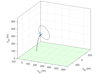
Figure 5: Visualization of the initial circular path.

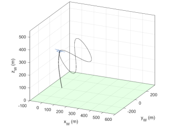
Figure 6: Visualization of the initial lemniscate path.

The initial state of the winch is found by assuming that the unstrained tether length equals with $||\bm{\mathbf{p}}_{\text{aircraft}}^{\mathcal{W}}||$, and the angular velocity of winch equals to the aircraft’s velocity along the z-axis in the $\tau$ frame.

$$\theta_{\text{winch}} =\frac{||\bm{\mathbf{p}}_{\text{aircraft}}^{\mathcal{W}}||}{r_{\text{winch}}}$$ (44)

$$\dot{\theta}_{\text{winch}}=\begin{pmatrix}c_{\lambda}c_{\eta}&s_{\lambda}c_{\eta}&s_{\eta}\end{pmatrix}R_{\mathcal{W}}^{\mathcal{O}}R_{\mathcal{O}}^{\mathcal{B}}\bm{\mathbf{v}}_{\text{aircraft}}^{\mathcal{B}}$$ (45)

Therefore, knowing all differential states leads to find algebraic variables $\bm{\mathbf{z}}$ for the circular and lemniscate paths by solving (32b) numerically. Lastly, the fictitious forces/torques and winch motor/generator torque are calculated through solving (32a) for all known $\bm{\mathbf{x}}$ and $\bm{\mathbf{z}}$.

IV Results and Discussion

The simulation results and optimal trajectories derived from the framework introduced in Section III using the model of Section II. Our focus lies on the megawatt-scale AWES within a two-fuselage aircraft with a wing span of $42.5m$ meters, as outlined in [19]. We investigated the lemniscate and circular paths for a medium wind speed of $15m/s$. To understand how a flexible tether affects the dynamics of AWESs from an optimization point of view, we simplify the quasi-static approach to make the tether rigid. The following results and optimal trajectories are derived from the optimization of the initial trajectories shown in Fig. 5 and Fig. 6, where the initial trajectories include six pumping cycles for circular trajectory and three pumping cycles for the lemniscate within $90s$. We discretize OCP into $N_{t}=270$ shooting nodes such that time step $h=\frac{T_{f}}{N_{t}}=0.3s$.

Considering the AWES model with both flexible and rigid tether is inherently index-1, the $\Psi(\bm{\mathbf{x}}(0))$ in (25) is considered as:

$$\Psi(\bm{\mathbf{x}}(0))=\begin{pmatrix}\bm{\mathbf{g}}(\bm{\mathbf{x}}_{0},\bm{\mathbf{z}}_{0})\\ \bm{\mathbf{p}}_{\text{aircraft}}^{\mathcal{W}}(t=0)-\bm{\mathbf{p}}_{0}\end{pmatrix}$$ (46)

where the first row is cold start [29] for the solution, and the second method can be used to constrain the initial point of the optimal path to a specific location, which could be either the starting point of the initial path or a point where the take-off maneuver is supposed to end. Constraining the initial position of the aircraft or any other quantities at this point is optional and can be implemented if there are specific physical or operational requirements.

The bounds of inequality constraints mentioned in (29a-29j), as well as states (differential and algebraic), and control inputs can be found in Table. I and Table. II respectively. As it is shown, the Euler angles are restricted to avoid singularities in solution through the flight. The critical assumption of non singular $\frac{\partial{\bm{\mathbf{g}}}}{\partial{\bm{\mathbf{z}}}}$ would be achieved if tether remained under tension $z_{3}>0$, and none of the tether lumped masses collide with the ground $z_{1}>0$. In Table. II, we chose the lower bounds of $z_{1}$ and $z_{3}$ greater zero to ensure those assumption always remain valid.

Table I: Inequality constraints bounds.

Description	Symbol	Min	Max	Unit
Tether force (aircraft)	$\|F_{\text{tether}}\|$	$1.31\times 10^{3}$	$1.665\times 10^{6}$	$N$
Aircraft position (y)	$p_{w}(y)$	-300	300	$m$
Aircraft position (z)	$p_{w}(z)$	100	600	$m$
Winch acceleration	$\dot{\omega}_{w}$	-5	5	$m/s^{2}$
Apparent velocity	$\|\bm{\mathbf{v}}_{\text{a}}\|$	10	90	$m/s$
Angle of attack	$\alpha$	-15	4.2	deg
Side slip angle	$\beta$	-10	10	deg
Corrected aero angles	(29g, 29h)	-15	15	deg
Corrected deflection (aileron)	(29i)	-35	35	deg
Tether collision avoidance	$\theta_{T}$	2	178	deg

Table II: Variables and controls bounds.

Description	Symbol	Min	Max	Unit
Linear velocity- x	$\bm{\mathbf{v}}_{\text{aircraft}}^{\mathcal{B}}(1)$	15	90	$m/s$
Linear velocity- y	$\bm{\mathbf{v}}_{\text{aircraft}}^{\mathcal{B}}(2)$	-60	60	$m/s$
Linear velocity- z	$\bm{\mathbf{v}}_{\text{aircraft}}^{\mathcal{B}}(3)$	-30	30	$m/s$
Angular velocities	$\bm{\mathbf{\omega}}_{\text{aircraft}}^{\mathcal{B}}$	-50	50	$deg/s$
Roll angle	$\phi$	$-0.7\pi/2$	$0.7\pi/2$	$rad$
Pitch angle	$\theta$	$-0.65\pi/2$	$0.65\pi/2$	$rad$
Yaw angle	$\psi_{\text{circular}}$	$-(2N_{W}+0.5)\pi$	$\pi/20$	$rad$
	$\psi_{\text{lemniscate}}$	$-\pi$	$\pi$	$rad$
Longitude	$\bm{\mathbf{q}}_{\text{s}}(1)$	$-\pi/2+\pi/20$	$\pi/2-\pi/20$	$rad$
Latitude	$\bm{\mathbf{q}}_{\text{s}}(2)$	$\pi/20$	$\pi/2-\pi/20$	$rad$
Distance	$\bm{\mathbf{q}}_{\text{s}}(3)$	60	1000	$m$
Torque (winch)	$\tau_{\text{generator}}$	0	$9\times 10^{7}$	$N.m$
Deflection (aileron)	$\delta_{\text{aileron}}$	-1	1	$rad$
Deflection (elevator)	$\delta_{\text{elevator}}$	-0.3316	0.3316	$rad$
Deflection (rudder)	$\delta_{\text{rudder}}$	-0.3316	0.3316	$rad$
Latitude ($m_{N}$ tether)	$\phi_{N}$	$\pi/50$	$\pi/2-\pi/50$	$rad$
Longitude ($m_{N}$ tether)	$\theta_{N}$	$-\pi/2$	$\pi/2$	$rad$
Force ($m_{N}$ tether)	$T$	$1.31\times 10^{3}$	$1.665\times 10^{6}$	$N$

To investigate the effect of the flexible tether model on path planning results, we compare our findings with those obtained using a rigid tether model. Previous studies on the optimization and path planning of rigid wing Airborne Wind Energy Systems (AWES) [4, 25, 6, 5] utilized a non-minimal coordinate model and considered the tether force as a constraint. However, it is impossible to incorporate that constraint within our model. Therefore, we introduced the following model, which allows us to contrast rigid and flexible tether modeling in path planning and optimal control problems.

IV-A Rigid tether model (simplified quasi-static approach)

To model a rigid tether, we simplified the flexible tether by neglecting the drag and gravity forces acting on the tether’s lumped masses. By eliminating these forces, which cause tether sag, we effectively made the tether rigid. Consequently, the force at the winch directly points to the aircraft’s position. Therefor, equation (14) simplifies to

$$m_{j}\ddot{\bm{\mathbf{p}}}_{j}=\bm{\mathbf{f}}_{j-1}-\bm{\mathbf{f}}_{j}$$ (47)

The roots of equation (22) represent the tether force magnitude and direction at the winch, which can be numerically found using the direct multiple shooting method, similar to the flexible tether case. To estimate the tether’s drag force act on the aircraft, We make use of a method similar to [11, 30], in which the drag force for the whole tether length is given by

$$\bm{\mathbf{f}}_{\text{tether}}^{\text{drag}}=-\frac{1}{8}\rho C_{D}ld_{\text{tether}}\|\bm{\mathbf{v}}_{a,\perp}\|\bm{\mathbf{v}}_{a,\perp}$$ (48)

where $l$ is the whole tether length. The drag force then applies to the aircraft by adding to (8a).

IV-B Simulation results

In this section, we discuss the generated optimal trajectories for both flexible and rigid tethers. As it is depicted in Fig. 5 and Fig. 6, the optimal paths for rigid and flexible tethers look similar. However, some differences are observed both in the traction and retraction phases. These discrepancies are more pronounced during the retraction and the transition between the traction and retraction phases.

Figure 7: Visualization of optimal trajectory with six circular pumping cycles for quasi-static and simplified tether models.

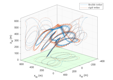
Figure 8: Visualization of optimal trajectory with three lemniscate pumping cycles for quasi-static and simplified tether models.

Moreover, the differences between the lemniscate trajectories generated for the rigid and flexible tethers are greater than their circular counterparts.

Despite the resemblance between the optimal trajectories for models with rigid and flexible tethers, there are notable differences in the control input signals and the estimated harvested power. In other words, the optimizer aims to maximize power by leading to maneuvers that increase lift. Therefore, while it is expected that the flying trajectories for both rigid and flexible tethers remain similar, the differences in tether dynamics and its effects on the aircraft cause changes in the control inputs.

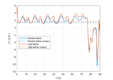
Figure 9: The mechanical power and its corresponded average power for optimal circular trajectories with quasi-static and simplified tether models.

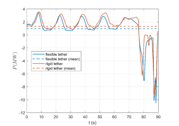
Figure 10: The mechanical power and its corresponded average power for optimal lemniscate trajectories with quasi-static and simplified tether models.

Although [11] claimed that the rigid tether model can accurately estimate power for one pumping cycle, the results shown in Fig. 10 and Fig. 9 demonstrate that it underestimates the effect of tether sag on the harvested power for both circular and lemniscate paths. The power in the pumping cycles of the model with a rigid tether is slightly higher than that of the model with a flexible tether, but there is a significant difference in power consumption during the retraction phase. Specifically, the energy required to return the aircraft to its initial position for a lemniscate trajectory is considerably higher than for a circular trajectory.

The tether force acting on the aircraft can be expressed based on its magnitude and two angles, which determine its direction in the body reference frame (Fig. 4). We previously described how we used one of those angles to avoid tether collides with aircraft. In Fig. 11 and Fig. 12, we quantify how tether sag might affect the direction of the tether force acting on the aircraft. The difference in angles during the retraction phase, for times after $75s$, represents the tether sag captured in the flexible tether model. It is evident that the tether sag in the lemniscate trajectory is greater than in the circular trajectory.

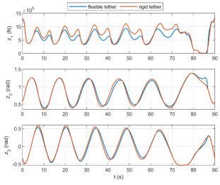
Figure 11: Tether force characteristics in body frame for the circular path.

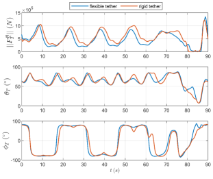
Figure 12: Tether force characteristics in body frame for the lemniscate path.

Addressing computational effort is essential for optimization purposes. The CPU time required to solve the optimal control problem on a PC with a 3.6 GHz AMD CPU and 32 GB RAM for circular and lemniscate trajectories is presented below. We assumed ten segments on the tether, which is sufficient to show the tether sag while keeping the computation time reasonable. A higher number of segments increases the model’s non-linearity and complexity, causing the computation time for the flexible tether to be higher than that for the rigid one. As can be seen by comparing in Fig. 14 and Fig. 13, the computation time for finding an optimal lemniscate trajectory is much higher than for the circular one. The more complicated and less well-defined forces and torques in lemniscate trajectories might be the reason for the increased computational effort.

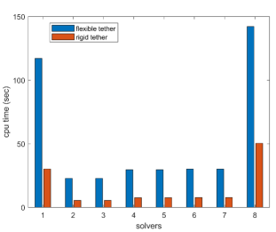
Figure 13: Computation cost of 90-second circular trajectories with quasi-static and simplified models of tether.

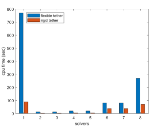
Figure 14: Computation cost of 90-second lemniscate trajectories with quasi-static and simplified models of tether.

Solver numbers one to eight are the homotopy solvers introduced in Algorithm 1. Solver numbers one and eight are the initial and final solvers, respectively. The intermediate solvers are divided into three homotopy stages: the first stage includes solvers two and three, which remove fictitious forces and torques; the second stage includes solvers four and five, which eliminate the propulsion force; and the third stage includes solvers six and seven, during which the cost function is adjusted for power production.

V Conclusion and Outlook

This work presents an optimal path planning framework to evaluate the performance of an airborne wind energy system (AWES) comprising a flexible tether, a winch, and a rigid-wing aircraft. The proposed framework generates paths with multiple pumping cycles using a homotopy approach. Unlike other research studies that employ an index-3 differential-algebraic system of equations (DAE) form and solve it using index reduction techniques, we employed a semi-explicit index-1 DAE form. This allows to add complementary constraints at the initial point to enhance the trajectory characteristics. Moreover, the quasi-static approach permits the use of a flexible tether model within an optimization problem without significantly increasing the number of states, as might occur with other lumped mass models used in literature.

To better understand how the trajectories generated with a flexible tether model differ from the ones generated with a rigid tether, a simplified version of the quasi-static approach was introduced to imitate the behavior of a rigid tether. Since the tether’s drag force was dropped as part of the simplification, we made use of a tether drag force estimation. The simulation results reveal that, although the optimal trajectories for a AWES with rigid and flexible tethers appear similar, the direction of the force exerted by the tether on the aircraft can differ significantly during the retraction phase. This difference leads to more pronounced mismatches between the optimal trajectories of the rigid and flexible tethers during the retraction phase compared to the pumping cycles. This can lead to the overestimation of harvested power for one pumping cycle up to 33%.

References

- [1] Uwe Ahrens, Moritz Diehl, and Roland Schmehl. Airborne wind energy. Springer Science & Business Media, 2013.
- [2] Chris Vermillion, Mitchell Cobb, Lorenzo Fagiano, Rachel Leuthold, Moritz Diehl, Roy S Smith, Tony A Wood, Sebastian Rapp, Roland Schmehl, and David Olinger. Electricity in the air: Insights from two decades of advanced control research and experimental flight testing of airborne wind energy systems. Annual Reviews in Control, 52:330–357, 2021.
- [3] Sébastien Gros and Moritz Diehl. Modeling of airborne wind energy systems in natural coordinates, pages 181–203. Springer, 2013.
- [4] Greg Horn, Sébastien Gros, and Moritz Diehl. Numerical trajectory optimization for airborne wind energy systems described by high fidelity aircraft models, pages 205–218. Springer, 2013.
- [5] Giovanni Licitra, Jonas Koenemann, Adrian Bürger, Paul Williams, Richard Ruiterkamp, and Moritz Diehl. Performance assessment of a rigid wing airborne wind energy pumping system. Energy, 173:569–585, 2019.
- [6] Jochem De Schutter, Rachel Leuthold, Thilo Bronnenmeyer, Elena Malz, Sebastien Gros, and Moritz Diehl. Awebox: An optimal control framework for single-and multi-aircraft airborne wind energy systems. Energies, 16(4):1900, 2023.
- [7] M Erhard, G Horn, and M Diehl. A quaternion-based model for optimal control of the sky-sails airborne wind energy system. zamm–journal of applied mathematics and mechanics (2016).
- [8] Nonlinear mpc of kites under varying wind conditions for a new class of large-scale wind power generators. International Journal of Robust and Nonlinear Control: IFAC-Affiliated Journal, 17(17):1590–1599, 2007.
- [9] Boris Houska and Moritz Diehl. Optimal control for power generating kites. In 2007 European Control Conference (ECC), pages 3560–3567. IEEE.
- [10] Thomas Stastny, Eva Ahbe, Manuel Dangel, and Roland Siegwart. Locally power-optimal nonlinear model predictive control for fixed-wing airborne wind energy. In 2019 American Control Conference (ACC), pages 2191–2196. IEEE.
- [11] EC Malz, J Koenemann, S Sieberling, and S Gros. A reference model for airborne wind energy systems for optimization and control. Renewable energy, 140:1004–1011, 2019.
- [12] Paul Williams. Cable modeling approximations for rapid simulation. Journal of guidance, control, and dynamics, 40(7):1779–1788, 2017.
- [13] Jingli Du, Chuanzhen Cui, Hong Bao, and Yuanying Qiu. Dynamic analysis of cable-driven parallel manipulators using a variable length finite element. Journal of Computational and Nonlinear Dynamics, 10(1):011013, 2015.
- [14] Mani Kakavand and Amin Nikoobin. Numerical simulation of tethered–wing power systems based on variational integration. Journal of Computational Science, 51:101351, 2021.
- [15] Uwe Fechner, Rolf van der Vlugt, Edwin Schreuder, and Roland Schmehl. Dynamic model of a pumping kite power system. Renewable Energy, 83:705–716, 2015.
- [16] Andrea Berra. Optimal control of pumping airborne wind energy systems without wind speed feedback. 2019.
- [17] Paul Williams, Sören Sieberling, and Richard Ruiterkamp. Flight test verification of a rigid wing airborne wind energy system. In 2019 American Control Conference (ACC), pages 2183–2190. IEEE, 2019.
- [18] Jonas Koenemann, Paul Williams, Soeren Sieberling, and Moritz Diehl. Modeling of an airborne wind energy system with a flexible tether model for the optimization of landing trajectories. IFAC-PapersOnLine, 50(1):11944–11950, 2017.
- [19] Dylan Eijkelhof and Roland Schmehl. Six-degrees-of-freedom simulation model for future multi-megawatt airborne wind energy systems. Renewable Energy, 196, 2022.
- [20] Joel A. E. Andersson, Joris Gillis, Greg Horn, James B. Rawlings, and Moritz Diehl. Casadi: a software framework for nonlinear optimization and optimal control. Mathematical Programming Computation, 11:1 – 36, 2018.
- [21] Modeling the Aircraft, chapter 2, pages 63–141. John Wiley & Sons, Ltd, 2015.
- [22] Sebastian Rapp, Roland Schmehl, Espen Oland, and Thomas Haas. Cascaded pumping cycle control for rigid wing airborne wind energy systems. Journal of Guidance, Control, and Dynamics, 42(11):2456–2473, 2019.
- [23] Lorenz T Biegler and Victor M Zavala. Large-scale nonlinear programming using ipopt: An integrating framework for enterprise-wide dynamic optimization. Computers & Chemical Engineering, 33(3):575–582, 2009.
- [24] Patrick R Amestoy, Iain S Duff, Jean-Yves L’Excellent, and Jacko Koster. Mumps: a general purpose distributed memory sparse solver. In International Workshop on Applied Parallel Computing, pages 121–130. Springer, 2000.
- [25] Sébastien Gros, Mario Zanon, and Moritz Diehl. A relaxation strategy for the optimization of airborne wind energy systems. In 2013 European Control Conference (ECC), pages 1011–1016. IEEE.
- [26] Wenbo He, Yunshen Huang, Jie Wang, and Shen Zeng. Homotopy method for optimal motion planning with homotopy class constraints. IEEE Control Systems Letters, 7:1045–1050, 2022.
- [27] Kristoffer Bergman and Daniel Axehill. Combining homotopy methods and numerical optimal control to solve motion planning problems. In 2018 IEEE Intelligent Vehicles Symposium (IV), pages 347–354. IEEE, 2018.
- [28] James Diebel. Representing attitude: Euler angles, unit quaternions, and rotation vectors. Matrix, 58(15-16):1–35, 2006.
- [29] U.M. Ascher and L.R. Petzold. Computer Methods for Ordinary Differential Equations and Differential-Algebraic Equations. Society for Industrial and Applied Mathematics (SIAM, 3600 Market Street, Floor 6, Philadelphia, PA 19104), 1998.
- [30] Ivan Argatov and Risto Silvennoinen. Efficiency of traction power conversion based on crosswind motion. Airborne Wind Energy, pages 65–79, 2013.