The stable ”Unstable Natural Media” due to the presence of turbulence

Abstract

The term ”unstable neutral media” (UNM) has traditionally been used to describe the transient phase formed between the warm and cold neutral hydrogen (HI) phases and has not been the focus of HI studies. However, recent observations suggest that the UNM phase not only has a significantly longer-than-expected lifetime but also occupies at least 20% to 40% of both the volume and mass fraction of HI. In this paper, we argue that the existence and dominance of the UNM can be explained by the presence of strong turbulence using an energy balance argument. The mass fraction of UNM is directly proportional to the turbulent velocity dispersion $\sigma_{v}$: mass fraction of UNM $\propto\sigma_{v}^{\frac{2n}{1+n}}$, where $n$ is the absolute value of the adiabatic index in the unstable phase. We discuss the implications of long-lived unstable thermal phases on ISM physics, including cold dense filament formation, cosmic ray acceleration, and measurement of galactic foreground statistics.

revtex4-1.clsrevtex4-2.cls

1 Introduction

The interstellar medium (ISM) is a complex mixture of gas, dust, and cosmic rays that plays a crucial role in the evolution of galaxies (McKee & Ostriker 1977, see also McKee & Ostriker (2007); Yuen et al. (2024)). The ISM can be divided into several phases, including the warm neutral medium (WNM), cold neutral medium (CNM), and unstable neutral medium (UNM, Heiles & Troland 2003). The WNM is characterized by temperatures of several thousand Kelvin and low densities, while the CNM has temperatures around 100 K and higher densities (Wolfire et al., 2003). The UNM is a dynamic and transitional phase that lies between the WNM and CNM and is susceptible to rapid changes in temperature and density (Field, 1965).

A widely-held assumption in the ISM community (McKee & Ostriker, 1977; Yuen et al., 2024) suggests that the unstable phase, as its name implies, is thermally unstable and has a relatively short lifetime. This argument is based on the fact that when the cooling timescale, influenced by various processes including radiative cooling, chemical reactions, and turbulence (Nakamura & Li, 2007), is balanced by the turbulence timescale. A rough estimation shows that the UNM lifetime is on the order of $O(1Myr)$. If this were the case, since the mass of the galaxy is conserved, the UNM fraction in our Milky Way should have declined very quickly, given that the lifetime of the galaxy is significantly longer than that of the UNM. However, numerical simulations suggest otherwise (Kim & Ostriker, 2018; Seifried et al., 2020a, b). Indeed, earlier literature with weak turbulence suggests that the fraction of UNM is on the order of a few percent (Audit & Hennebelle, 2005). However, it has been observationally suggested (Kalberla & Kerp, 2009; Murray et al., 2018) that UNM occupies at least 20% of the total fraction (Murray et al., 2018; McClure-Griffiths et al., 2023), with some reports of up to 40% (Kalberla & Haud, 2018), suggesting that there are some sort of ’heat source’ continually elevating the CNM to warmer phases.

One of the leading hypotheses is that the presence of turbulence acts like a heat source, maintaining the high fraction of UNM observed. Recent studies have shown that turbulence can significantly impact the fraction and stability of the UNM (Audit & Hennebelle, 2005; Hennebelle & Audit, 2007; Hennebelle et al., 2007). Moreover, new evidence suggests that turbulence plays an important role in shaping the power spectrum (Yuen et al., 2022) and anisotropy (Ho et al., 2023) of the multiphase ISM. In fact, earlier literature (Cho et al., 2003) suggests that turbulence can transport heat much more effectively than the native thermal conduction rate, and in the case of the ISM, it is a few orders of magnitude stronger than its thermal counterpart. However, a quantitative analysis of how and why this leads to a large fraction of UNM is still unknown.

In this paper, we discuss how turbulence can extend the lifetime of the unstable phase, making it appear stable compared to the radiative cooling timescale. In Section 2, we briefly review the relevant timescales for multiphase physics. In Section 3, we utilize the energy argument to explain why turbulence can significantly enhance the UNM fraction as observed in the sky. In Section 4, we discuss our numerical results. In Section 5, we summarize and conclude our paper.

2 Review of timescale argument in formation and stability of unstable phase

2.1 Important time scale and length scale in Multi-phase ISM

When discussing the physics of multi-phase ISM, the cooling effect is considered as one of the dominating process in studying the dynamics of ISM. To demonstrate that, one of the classical argument is coming from the timescale comparison. The multi-phase ISM can be treated as a fluid, and for that, the dynamical timescale $\tau_{d}$ determines the importance of fluid motion. For cooling effect, we can define a cooling time scale $\tau_{c}$. They can be defined as :

$$\tau_{c}=\frac{E}{\dot{E_{c}}},$$ (1)

$$\tau_{d}=\frac{L}{c_{s}},$$

where $E,\dot{E_{c}},L,c_{s}$ are the internal energy of the fluid element, cooling rate, length scale of the ISM and speed of sound. The timescales can be interpreted as the time required for a process become important. The shorter one is more important than a longer one.

Assuming the idea gas law and plugging in the usual ISM parameter, we can then estimate the two timescales. For example, assuming the ISM temperature $T=1500K$, $L=100pc$, and $\dot{E_{c}}=2\times 10^{-26}ergs^{-1}$ and density $n_{H}=2cm^{-3}$, we arrive with an order of magnitude estimate of $\tau_{d}\sim O(10Myr)$ and $\tau_{c}\sim O(Myr)$, indicating that the cooling finishes almost instantly after the heat exchange due to fluid motion. We neglect the effect from thermal conduction as the corresponding characteristic length scale is at the order of $10^{-2}$ pc, meaning that the natural thermal conduction only plays a minor role on the scale of ISM, consistent with the estimate in Cho et al. (2003).

In this interpretation, we observe that the internal energy of fluid element ultimately determined by the cooling function. The multiphase gas will be stabilize very quickly roughly at the order of cooling timescale, where a static fraction of warm and cold gas mixture are formed without much mixing, which is the scenario outlined as early as Wolfire et al. (2003).

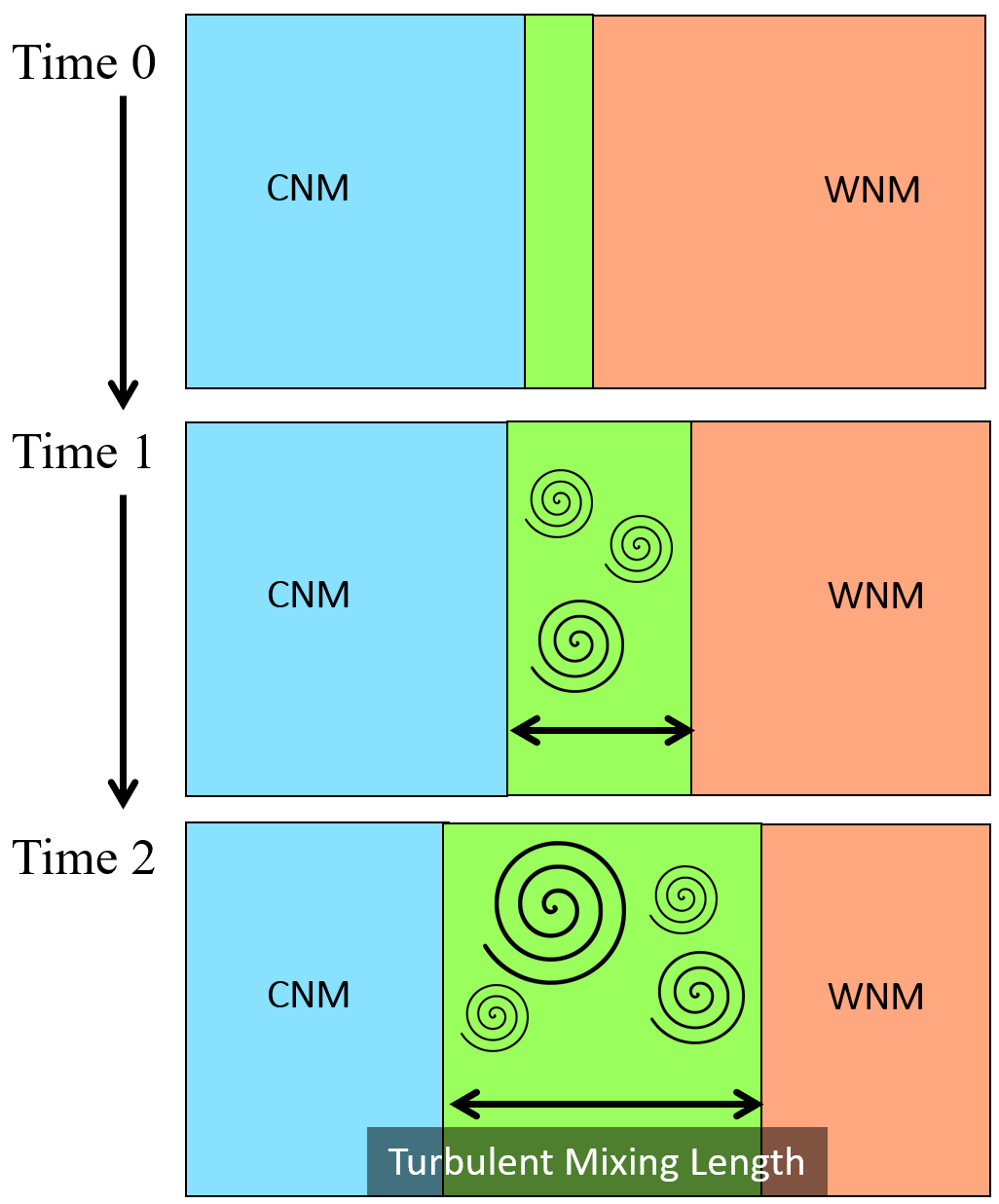
Figure 1: Illustration of Cold-Heat End Model, The formation of UNM under temperature gradient and turbulence mixing.

2.2 Turbulent mixing effect

However, observational study shows that the multi-phase ISM is turbulent (See, e.g. Yuen et al. 2022) and one should consider the effect arising from turbulent motion. Prior simulations observed that a substantial amount of unstable phases are produced when turbulence is generated, but the actual fraction of unstable phases are not in agreement, despite a rough range of estimate of $20-28\%$ is observed across different simulations(Seifried et al., 2020a, b; Fielding et al., 2023), but some of other simulations has the unstable phases up to $60\%$ (Kritsuk et al., 2017, 2018). Similar variation is also raised from the observational side (Murray et al., 2018; Kalberla et al., 2020; McClure-Griffiths et al., 2023).

For a fully turbulent medium, turbulence mixing effect plays an important role in transferring heat of the fluid, as turbulence heat transport known to be more efficient than natural thermal transport in the case of ISM environment(Cho et al., 2003). To quantify the turbulence mixing, we follow the argument from last section and consider its timescale, which defined as :

$$\tau_{t}=\frac{l}{v},$$ (2)

where $l,v$ are the eddies scale and length scale at the size of unstable phase. One could link the two observables via Kolmogorov (1941) scaling $v\propto l^{1/3}$ and arrive with:

$$\tau_{t}\sim\tau_{0}(\frac{l}{L})^{2/3},$$ (3)

where $\tau_{0}=L/V_{0}$ denoting the turbulence mixing time at timescale given the velocity $V_{0}$ at scale L. One could see that the turbulence mixing effect is scale dependent and decreasing in smaller scale. We consider at a smaller length scale $l_{t}$, $\tau_{t}$ would decrease down to the magnitude of $\tau_{c}$. To estimate the value, we assume that at the unstable phase it is mildly trans-Alfvenic, i.e. $V_{0}\sim c_{s}$, and the timescale estimate gives:

$$(\frac{\tau_{c}}{\tau_{d}})^{3/2}\sim(\frac{l_{t}}{L}).$$ (4)

For the case of $\tau_{c}/\tau_{d}\sim 0.1$ that we adopted earlier ($\tau_{d}\sim 10Myr,\tau_{c}\sim Myr$), $l_{t}$ is about $3pc$, meaning that at this scale, the effect of turbulence mixing effect play a comparable role with cooling effect. Fig.1 shows a cartoon on how the turbulence mixing actually works: When turbulence is in play, there is an intermediate layer with the width be the turbulence mixing length $l_{t}$ in which the energy is supported by turbulence free energy. While the two stable phases have no heat loss, fluid elements transported into the mixing layer are subjected to imbalanced heating and cooling which is reflected by the negative adiabatic index as seen in multiphase numerical simulation, which we shall discuss in the next section.

3 Energy balance argument

From §2, we observe that the turbulence mixing effect dominates over thermal conduction in terms of heat transport. However, we do not see why the argument in the previous section could explain the potential very long lifetime and large fraction of UNM. The reason is because the modern MHD turbulence theory (Goldreich & Sridhar, 1995; Maron & Goldreich, 2001; Cho & Lazarian, 2003) assumes that the only energy sink for the plasma modes are dissipation (from ion-neutral damping in the case of ISM, see Yan & Lazarian (2004); Xu et al. (2015)). However, in the case of multiphase media, there is an additional energy sink that allows the turbulence to behave differently during phase transition: the abnormal $P\propto\rho^{-n}(n>0)$ unstable phase equation of state (EoS). While we will postpone the full analysis to the upcoming paper (Yuen et al. in prep) in exploring the quantitative values of $n$ as expected for a given turbulence model, it is crucial to consider how turbulence energy transfer is changed when having the abnormal EoS.

Let us consider the scale of UNM with thickness of $\sim 1pc$, which is evidently larger than the ion-neutral decoupling scale (Li et al., 2010; Hezareh et al., 2010; Houde et al., 2011; Xu et al., 2015). The energy equation can be written as ($\epsilon=\rho v^{2}/2$):

$$\frac{\partial\epsilon}{\partial t}+\nabla\cdot((2\epsilon+P){\bf v})=\rho\Lambda-\rho^{2}T^{1/2}\Gamma e^{-184/T}$$ (5)

where $\rho\Lambda$ is the radiative heating function and $\rho^{2}T^{1/2}\Gamma e^{-184/T}$ is the radiative cooling function. Both $\Lambda$ and $\Gamma$ can be approximated as roughly constants (Zweibel & Josafatsson, 1983) in the length scales that we are considering. The rough variation of the heating and cooling functions as the temperature changes is shown in Fig 3. A general trend for the heating and cooling functions are: in the case of WNM and CNM they are roughly balanced, and an adiabatic EoS is enforced. For UNM, the cooling function is significantly stronger than that of the heating function. Notice that we are assuming that our mixture of gases are in the regime 3 of Wolfire et al. (2003), i.e., the mean density (so as pressure) lies in between the maximum warm phase density and the minimum of cold phase density. In our discussion, we can therefore combine both CNM and WNM together, while separating that of UNM for dedicated analysis. Our ultimate goal is to obtain the following parameter:

$$\chi_{UNM,mass}=\frac{m_{UNM}}{1-m_{UNM}}$$ (6)

where

$$m_{UNM}=\frac{\int_{min(T):\Lambda=\rho T^{1/2}\Gamma e^{-184/T}}^{max(T):\Lambda=\rho T^{1/2}\Gamma e^{-184/T}}dT\rho(T)}{\int dT\rho(T)}$$ (7)

One of the major principles for us to move forward is that all three phases shared the same Kolmogorov scaling (Yuen et al., 2022). i.e their $\delta v$ strictly obeys $\delta v\propto l_{\perp}^{1/3}$. Noticing that the solution of the integral in Eq.7 is Equation of State dependent. At the moment, we will assume an isotropic scaling law to provide a first order estimate and defer the anisotropy argument in later publication.

From Yuen et al. (2022) we observe that the energy transfer rate $\frac{\partial\epsilon}{\partial t}$ is roughly constant since apparently a Kolmogorov-like spectrum is maintained over the scales of transitions. We can proceed with Eq.5 by expressing $P$ and $T$ via the polytropic EoS with negative adiabatic index and ideal gas law, respectively:

$$P =C\rho^{-n}\quad(n>0)$$ (8)

$$T =\frac{P}{\rho k_{B}}=\frac{C}{k_{B}}\rho^{-n-1}$$

for some constant C. The typical value of $n\in(0,1)$ in observation (Kalberla & Haud, 2018), but in this analysis we did not impose any restrictions on $n$ except requiring $n>0$. We first approximate the range of values of $T$ in relation to $n$:

$$C^{\prime}T^{\frac{n-1}{2(n+1)}}\approx e^{184/T}$$ (9)

for some constant $C^{\prime}$, denoting these two solutions as $T_{1,2}$ that correspond to the cold and warm gas density, respectively. Then Eq.7 can be written as :

$$m_{UNM} \propto\int_{T_{1}}^{T_{2}}dT(\frac{C}{k_{B}})^{\frac{1}{n+1}}T^{\frac{-1}{n+1}}$$ (10)

$$=(\frac{C}{k_{B}})^{\frac{1}{n+1}}\frac{n}{n+1}(T_{2}^{\frac{n}{n+1}}-T_{1}^{\frac{n}{n+1}})$$

where from observation we know $T_{2}\gg T_{1}$ ($T_{1}\approx 200K,T_{2}\approx 5000K$), therefore the $T_{1}$ part can be safely ignored in our order-of-magnitude estimates.

What remains is to relate $T_{1,2}$ with turbulence velocity $v$. Assuming all the turbulence energy went into the support of the negative adiabatic EoS:

$$\frac{2\rho v^{3}}{l}\sim\frac{C\rho^{-n}v}{l}$$ (11)

Taking Kolmogorov scaling, we have $v^{3}/l\approx\text{const}$

$$v^{-2} \propto l^{-2/3}\propto\rho^{1+n}\propto T^{-1}$$ (12)

$$\rightarrow T^{1/2} \sim v$$

The mass fraction of UNM is given by ($n>0$, see Footnote 1):

$$\chi_{UNM,mass}=\frac{\text{const}\times v^{\frac{2n}{1+n}}}{1-\text{const}\times v^{\frac{2n}{1+n}}}$$ (13)

The r.m.s. sonic Mach number of the system is proportional to $v$. Therefore we expect that when the UNM fraction is not dominant (i.e. $<50\%$), the mass fraction of UNM has the following scaling to the turbulent velocity $v$ (which is measured by $\sigma_{v}$ in simulation):

$$\chi_{UNM,mass}\propto v^{\frac{2n}{1+n}}$$ (14)

For typical $n$ value of $0.3-0.4$ (i.e. $P\propto\rho^{-0.3}\text{ to }\rho^{-0.4}$), the mass fraction of UNM is about $v^{0.46}\text{ to}\>v^{0.57}$.

Simulation	$\sigma_{v}\>[km\>s^{-1}]$	$N^{3}$	$L\>[pc]$	$\rho$ $\,[m_{H}\,cm^{-3}]$
M0	0.12	$512^{3}$	$100$	$3$
M1	0.22
M2	0.45
M3	0.93
M4	1.63
M5	3.01
M6	4.86

Table 1: Simulation parameters, from the left; velocity dispersion $\sigma_{v}$ (in km/s), Resolution $N^{3}$, Length Scale $L$, and mean number density of atomic hydrogen $n_{H}$.

4 Numerical Method & Result

4.1 Numerical Simulations

To compare the result in §2, we use the 3D MHD multi-phase simulations generated from the MHD code Athena++, which were also being used in Yuen et al. (2021) and Ho et al. (2023). For the initial state, we set up a 3D periodic turbulence box with the length of 100 pc and we are assuming the fluid represents the bulk neutral hydrogen in the interstellar media. We adopt the realistic cooling and heating function proposed by Koyama & Inutsuka (2002). The simulation was originally constant in density and was driven via spectral velocity perturbation in the Fourier space.

We set up a few simulations with the conditions similar to the realistic multi-phase neutral hydrogen gases with mass/volume fractions being consistent with observations. We shall define the gas as the cold phase when the temperature of the gas is below 200K while those above 5500K as to warm phase, while the gas in between is the unstable phase. At around 50 Myr the turbulence box has produced a realistic multi-phase medium, which the parameters are listed in Tab.1. For our current case study, the cooling lengthscale is roughly $\sim L_{inj}/10$. Therefore, simulations at resolution of $512^{3}$ is sufficient for the current studies.

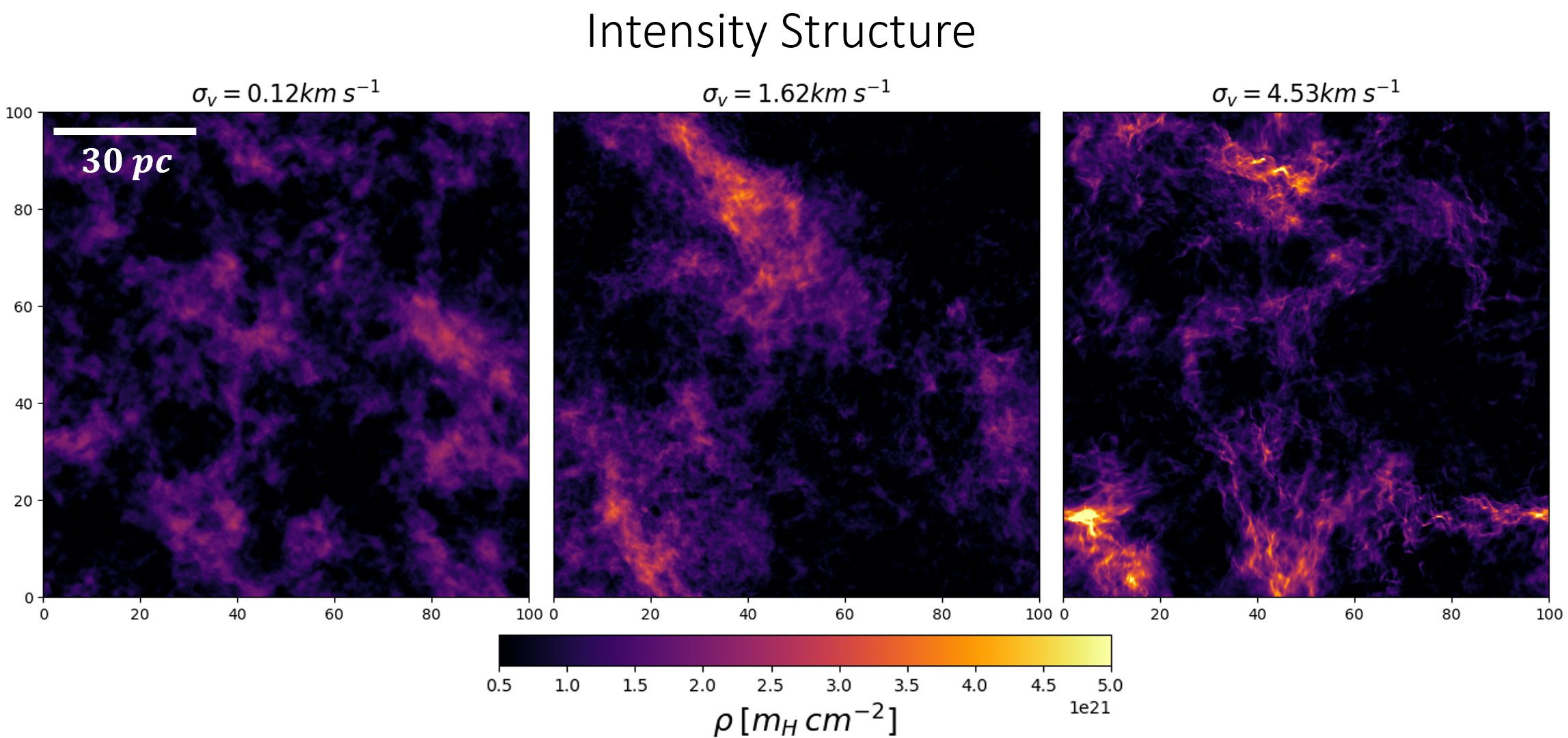
Figure 2: Three panels showing the structure of multiphase HI density projection when we vary the velocity dispersion.

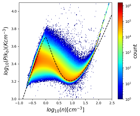
Figure 3: A plot showing how the phase diagram of the simulations vary as functions of the injection velocity. The dashed curve is the equilibrium curve (i.e. heating = cooling in the energy evolution (R.H.S. of Eq.5=0) with the (negative) adiabatic index $n\approx 0.5$. However, most of the fluctuations do not follow the equilibrium curve with a numerical adiabatic index of $n\approx 0.3$.

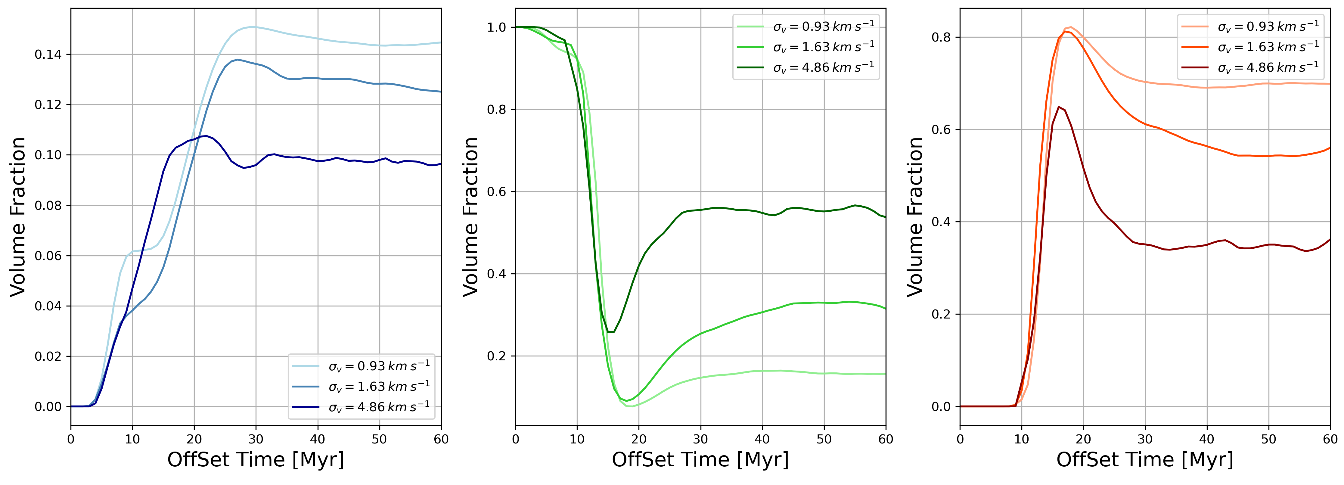
Figure 4: A set of figures showing how the volume fraction of the three phases (left: cold, medium: unstable, right: warm) vary across offset time for three different cases of turbulent velocity dispersion. The offset time defined as the time when thermal instability happens.

Fig. 2 shows how does the intensity structure (density projected along of sight) looks like in three cases of multiphase media with different injection velocity dispersion $\sigma_{v}=0.12,1.62,\text{ and }4.53\text{kms}^{-1}$. We can see visually from Fig.2 that the increase of injection velocity have apparent visual effect on the distribution of density features in the simulation domain, very similar to the situation that outlined in Yuen & Lazarian (2020): When the injection velocity is larger, the effective sonic Mach number is also larger, and as a result, thin features can be formed very easily under strong turbulence compression.

We also present the phase diagrams of these simulations as in Fig. 3. We can see that stronger turbulence makes the thermal curve much more steepened, which is a well-known result from the community (Kritsuk et al., 2017; Kim & Ostriker, 2018). By observation, the numerical value of the adiabatic index $n$ in the unstable phase is about 0.3. We expect that the numerical value of $n$ to be shallower than the equilibrium curve (dashed line of Eq.3) due to strong thermal instability.

4.2 Numerical Verification of the fraction estimation

How does the turbulent velocity affects the fraction of the three phases? In Fig.4 we show how the fraction of three phases vary as a function of offset time for three different cases of turbulent velocity. We observe a few different things that are very apparent from these simulations: (i) when the injection velocity increases, the volume fraction of unstable phase increases. (ii) Both volume fractions of cold and warm phases decrease as the turbulent velocity increases, (iii) the volume fraction of cold phase enters the equilibrium earlier when the turbulence velocity amplitude is larger, (iv) all three phases have entered equilibrium stage for an extended amount of lifetime. These qualitative facts suggest that the increases presence of turbulence allow the originally thermally unstable phase becomes particularly stable in our study.

How does the fraction stability be achieved? Earlier proposal (Wolfire et al., 2003; McKee & Ostriker, 2007) suggests that materials are cycling between the cold and warm phases, which appears to make the unstable phase be in large fraction despite the lifetime of the thermally unstable materials are dynamically short. Fig.4 seems to suggest that both fractions of cold and warm phases are reduced as the turbulence strength increases, implying that the material cycling argument could work. Indeed, the increased presence of thermally unstable phase (Ho et al., 2023) imposes additional forces to cold phases. When UNM fraction increases, the thermal instability creates more CNM, creating an equilibrium in between.

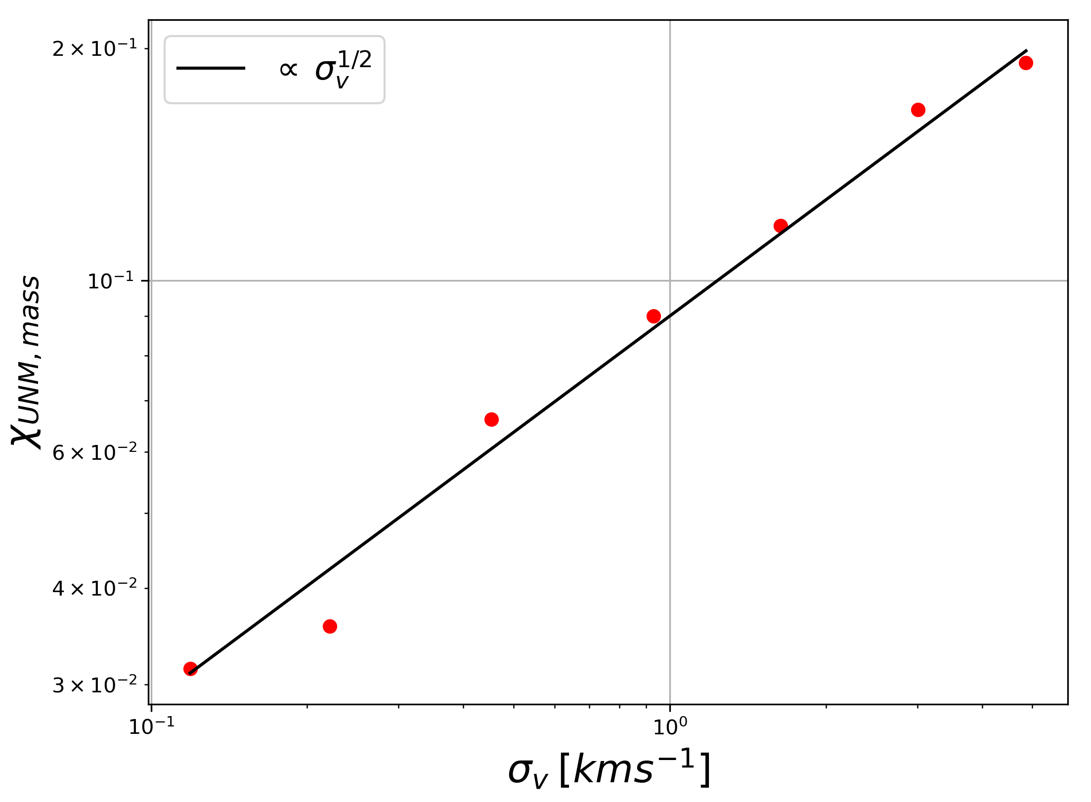
Figure 5: A figure showing how the time averaged mass fraction of unstable phase varies as a function of velocity dispersion. For each data point, it takes the average of 50 Myr.

From the qualitative perspective we understand that turbulence fueled the stability of thermally unstable phase, but did our quantitative prediction (Eq.13) be realized in the simulation? In Fig. 5 we show the time averaged mass fraction of the UNM as a function of $\sigma_{v}$, velocity dispersion, which is a direct proxy of $v$. Notice that in a simulation with given initial density and pre-defined heating and cooling functions, we already know approximately the mean density of the unstable phase. Fig.5 shows that the variation of mass fraction for the unstable phase has a power-law relation to the injection velocity. In our case the relation is roughly $\chi_{UNM}\propto v^{1/2}$, meaning that $n\approx 1/3$, matching the slopes in the phase diagram we see from Fig.3.

5 Discussion and Conclusion

In the previous paper of our series (Ho et al., 2023), we revealed that the presence of negative adiabatic index will create additional, short-range gravity-like pressure term that confines the cold neutral media, i.e. long filaments (Clark et al. 2015; Xu et al. 2019, see Yuen et al. 2024 for a review) that are longer than the threshold of the thermal instability are not stable. In the current paper we revealed that it is turbulence that supports this action, and a stronger level of turbulence will actually make the instability strong, instead of weaker. In other words, the density map of multiphase media under the combined action of heating and cooling functions will appear to be much more scattered, which agrees with our observation in Fig.2. We want to emphasize that, isothermal simulations with plasma conditions similar to that in our simulated cold neutral media will not be that scattered, which can be readily seen in some state-of-the-art numerical simulations (e.g. Federrath et al. 2021). It is a combined action of the turbulence and phase effect that drives both the dynamics (Ho et al., 2023) and the unstable fraction, which is presented in the current paper, to be very different from the isothermal counterpart.

We also want to emphasize that the micro-physics of unstable media is very important in further quantifying the dynamics of ISM (Fielding et al. 2023; Kritsuk et al. 2024). One of the most important development in the studies of ISM is the inclusion of low energy (1-200GeV) cosmic rays into the multiphase ISM system (Habegger et al., 2024; Guo et al., 2024). It is observed that the compressive part of the turbulence energy, presumably most effectively generated by thermal instability, is taken away from the ISM in energizing (heating) the cosmic ray, leading to a runaway energy growth of cosmic ray energy. In the context of MHD turbulence theory, it is the fast modes that energize the cosmic rays most efficiently at that energy range (Yan & Lazarian, 2002). Numerically it is reported that fast modes are dominant in the multiphase ISM (Beresnyak, 2024). We want to stress the fact that the dominance of fast mode also significantly modify the statistics of turbulence, particularly in the form of intermittancy (Ho & Lazarian, 2021), in which it accelerates cosmic rays (Kempski & Quataert, 2022) and modifies the observed polarization (Pavaskar et al., 2024). Furthermore, it appears to be sufficient in modifying the statistics of E/B modes on the sky (Kritsuk et al. 2018, 2024).

The microphysics that we are investigating in this paper is incomplete. Despite we know that the phase change can lead to the spatial deformation of CNM (Ho et al., 2023), and turbulence can also fueled up the phase changes (the current paper), we still do not know how the heat within the CNM is transported, particularly if we include cosmic ray feedback (Habegger et al., 2024). We will discuss this particular piece of physics in the later papers.

As a conclusion, in this paper we present a viable scenario for unstable phase to be dynamically stable compared to the dynamical time of radiative cooling and cloud evolution time, which can potentially explain the large unstable fraction as observed in Murray et al. (2018). In short:

1. The fraction of UNM is maintained decades ($>20Myr$) over the cooling time ($\sim 2Myr)$. (Fig.4) when turbulence is present.

2. When we increase the turbulence levels, more fluid parcels fall into the thermally unstable phase. Analytically, the mass fraction of UNM is $\propto v^{\frac{2n}{1+n}}$ (Eq.14)

3. In particular, in our numerical simulations we observe that Eq.14 is a precise prediction of mass fraction of UNM (Fig.5).

Acknowledgments. KHY acknowledges Hui Li for providing extensive suggestions and comments on the conduction physics of cold filaments on the sky, particular for his insight on thermal and turbulent anisotropic conduction. KWH acknowledges Chang-Goo Kim for providing extensive suggestions and comments on the paper during the 2023 Athena++ workshop. KWH & AL acknowledge the support the NSF AST 1816234, NASA TCAN 144AAG1967, NSF grant AST 1212096 and NASA grant NNX14AJ53G. The research presented in this article was supported by the LDRD program of LANL with project # 20220107DR (KWH) & 20220700PRD1 (KHY), and a U.S. DOE Fusion Energy Science project. This research used resources from the LANL Institutional Computing Program (y23_filaments), supported by the DOE NNSA Contract No. 89233218CNA000001. This research also used resources of NERSC with award numbers FES-ERCAP-m4239 (PI: KHY) and m4364 (PI: KWH). This research was supported in part by grant NSF PHY-2309135 to the Kavli Institute for Theoretical Physics (KITP).

Software Julia-v1.8.2/ Julia-v1.8.3, Jupyter/miniconda3, C++ 11, MHDFlows (Ho, 2022)

References

- Audit & Hennebelle (2005) Audit, E., & Hennebelle, P. 2005, A&A, 433, 1, doi: 10.1051/0004-6361:20041474
- Beresnyak (2024) Beresnyak, A. 2024, in American Astronomical Society Meeting Abstracts, Vol. 244, American Astronomical Society Meeting Abstracts, 114.02
- Cho & Lazarian (2003) Cho, J., & Lazarian, A. 2003, MNRAS, 345, 325, doi: 10.1046/j.1365-8711.2003.06941.x
- Cho et al. (2003) Cho, J., Lazarian, A., Honein, A., et al. 2003, ApJ, 589, L77, doi: 10.1086/376492
- Clark et al. (2015) Clark, S. E., Hill, J. C., Peek, J. E. G., Putman, M. E., & Babler, B. L. 2015, Phys. Rev. Lett., 115, 241302, doi: 10.1103/PhysRevLett.115.241302
- Federrath et al. (2021) Federrath, C., Klessen, R. S., Iapichino, L., & Beattie, J. R. 2021, Nature Astronomy, 5, 365, doi: 10.1038/s41550-020-01282-z
- Field (1965) Field, G. B. 1965, ApJ, 142, 531, doi: 10.1086/148317
- Fielding et al. (2023) Fielding, D. B., Ripperda, B., & Philippov, A. A. 2023, ApJ, 949, L5, doi: 10.3847/2041-8213/accf1f
- Goldreich & Sridhar (1995) Goldreich, P., & Sridhar, S. 1995, ApJ, 438, 763, doi: 10.1086/175121
- Guo et al. (2024) Guo, F., Seo, J., Yuen, K. H., & Ho, K. W. 2024, in American Astronomical Society Meeting Abstracts, Vol. 244, American Astronomical Society Meeting Abstracts, 123.02
- Habegger et al. (2024) Habegger, R., Ho, K. W., Yuen, K. H., & Zweibel, E. G. 2024, arXiv e-prints, arXiv:2403.07976, doi: 10.48550/arXiv.2403.07976
- Heiles & Troland (2003) Heiles, C., & Troland, T. H. 2003, ApJ, 586, 1067, doi: 10.1086/367828
- Hennebelle & Audit (2007) Hennebelle, P., & Audit, E. 2007, A&A, 465, 431, doi: 10.1051/0004-6361:20066139
- Hennebelle et al. (2007) Hennebelle, P., Audit, E., & Miville-Deschênes, M. A. 2007, A&A, 465, 445, doi: 10.1051/0004-6361:20066141
- Hezareh et al. (2010) Hezareh, T., Houde, M., McCoey, C., & Li, H.-b. 2010, ApJ, 720, 603, doi: 10.1088/0004-637X/720/1/603
- Ho (2022) Ho, K. W. 2022, MHDFlows.jl, 0.2.1b, Zenodo, doi: 10.5281/zenodo.8242702
- Ho & Lazarian (2021) Ho, K. W., & Lazarian, A. 2021, ApJ, 911, 53, doi: 10.3847/1538-4357/abe713
- Ho et al. (2023) Ho, K. W., Yuen, K. H., & Lazarian, A. 2023, MNRAS, 521, 230, doi: 10.1093/mnras/stad481
- Houde et al. (2011) Houde, M., Hezareh, T., Li, H.-B., & Phillips, T. G. 2011, Modern Physics Letters A, 26, 235, doi: 10.1142/S021773231103502X
- Kalberla & Haud (2018) Kalberla, P. M. W., & Haud, U. 2018, A&A, 619, A58, doi: 10.1051/0004-6361/201833146
- Kalberla & Kerp (2009) Kalberla, P. M. W., & Kerp, J. 2009, ARA&A, 47, 27, doi: 10.1146/annurev-astro-082708-101823
- Kalberla et al. (2020) Kalberla, P. M. W., Kerp, J., & Haud, U. 2020, A&A, 639, A26, doi: 10.1051/0004-6361/202037602
- Kempski & Quataert (2022) Kempski, P., & Quataert, E. 2022, MNRAS, 514, 657, doi: 10.1093/mnras/stac1240
- Kim & Ostriker (2018) Kim, C.-G., & Ostriker, E. C. 2018, ApJ, 853, 173, doi: 10.3847/1538-4357/aaa5ff
- Kolmogorov (1941) Kolmogorov, A. 1941, Akademiia Nauk SSSR Doklady, 30, 301
- Koyama & Inutsuka (2002) Koyama, H., & Inutsuka, S.-i. 2002, ApJ, 564, L97, doi: 10.1086/338978
- Kritsuk et al. (2024) Kritsuk, A., Ho, K. W., Yuen, K. H., & Flauger, R. 2024, in American Astronomical Society Meeting Abstracts, Vol. 244, American Astronomical Society Meeting Abstracts, 215.02
- Kritsuk et al. (2018) Kritsuk, A. G., Flauger, R., & Ustyugov, S. D. 2018, Phys. Rev. Lett., 121, 021104, doi: 10.1103/PhysRevLett.121.021104
- Kritsuk et al. (2017) Kritsuk, A. G., Ustyugov, S. D., & Norman, M. L. 2017, New Journal of Physics, 19, 065003, doi: 10.1088/1367-2630/aa7156
- Li et al. (2010) Li, H.-b., Houde, M., Lai, S.-p., & Sridharan, T. K. 2010, ApJ, 718, 905, doi: 10.1088/0004-637X/718/2/905
- Maron & Goldreich (2001) Maron, J., & Goldreich, P. 2001, ApJ, 554, 1175, doi: 10.1086/321413
- McClure-Griffiths et al. (2023) McClure-Griffiths, N. M., Stanimirović, S., & Rybarczyk, D. R. 2023, ARA&A, 61, 19, doi: 10.1146/annurev-astro-052920-104851
- McKee & Ostriker (2007) McKee, C. F., & Ostriker, E. C. 2007, ARA&A, 45, 565, doi: 10.1146/annurev.astro.45.051806.110602
- McKee & Ostriker (1977) McKee, C. F., & Ostriker, J. P. 1977, ApJ, 218, 148, doi: 10.1086/155667
- Murray et al. (2018) Murray, C. E., Stanimirović, S., Goss, W. M., et al. 2018, ApJS, 238, 14, doi: 10.3847/1538-4365/aad81a
- Nakamura & Li (2007) Nakamura, F., & Li, Z.-Y. 2007, in Triggered Star Formation in a Turbulent ISM, ed. B. G. Elmegreen & J. Palous, Vol. 237, 306–310, doi: 10.1017/S1743921307001640
- Pavaskar et al. (2024) Pavaskar, P., Yuen, K. H., Yan, H., & Malik, S. 2024, arXiv e-prints, arXiv:2405.17985. https://arxiv.org/abs/2405.17985
- Seifried et al. (2020a) Seifried, D., Haid, S., Walch, S., Borchert, E. M. A., & Bisbas, T. G. 2020a, MNRAS, 492, 1465, doi: 10.1093/mnras/stz3563
- Seifried et al. (2020b) Seifried, D., Walch, S., Weis, M., et al. 2020b, MNRAS, 497, 4196, doi: 10.1093/mnras/staa2231
- Wolfire et al. (2003) Wolfire, M. G., McKee, C. F., Hollenbach, D., & Tielens, A. G. G. M. 2003, ApJ, 587, 278, doi: 10.1086/368016
- Xu et al. (2019) Xu, S., Ji, S., & Lazarian, A. 2019, ApJ, 878, 157, doi: 10.3847/1538-4357/ab21be
- Xu et al. (2015) Xu, S., Lazarian, A., & Yan, H. 2015, ApJ, 810, 44, doi: 10.1088/0004-637X/810/1/44
- Yan & Lazarian (2002) Yan, H., & Lazarian, A. 2002, Phys. Rev. Lett., 89, 281102, doi: 10.1103/PhysRevLett.89.281102
- Yan & Lazarian (2004) —. 2004, ApJ, 614, 757, doi: 10.1086/423733
- Yuen et al. (2024) Yuen, K. H., Ho, K. W., Law, C. Y., & Chen, A. 2024, Reviews of Modern Plasma Physics, invited review, arXiv:2404.19101, doi: 10.1007/s41614-024-00156-5
- Yuen et al. (2022) Yuen, K. H., Ho, K. W., Law, C. Y., Chen, A., & Lazarian, A. 2022, ApJ, submitted, arXiv:2204.13760
- Yuen et al. (2021) Yuen, K. H., Ho, K. W., & Lazarian, A. 2021, ApJ, 910, 161, doi: 10.3847/1538-4357/abe4d4
- Yuen & Lazarian (2020) Yuen, K. H., & Lazarian, A. 2020, ApJ, 898, 65, doi: 10.3847/1538-4357/ab9307
- Zweibel & Josafatsson (1983) Zweibel, E. G., & Josafatsson, K. 1983, ApJ, 270, 511, doi: 10.1086/161144