Convergence of Sinkhorn’s Algorithm for Entropic Martingale Optimal Transport Problem

Abstract

In this paper, we study the Entropic Martingale Optimal Transport (EMOT) problem on $\mathbb{R}$. We begin by introducing the dual formulation and prove the exponential convergence of Sinkhorn’s algorithm on the dual potential coefficients. Our analysis does not require prior knowledge of the optimal potential and confirms that there is no primal-dual gap. Our findings provide a theoretical guarantee for solving the EMOT problem using Sinkhorn’s algorithm. In applications, our result provides insight into the calibration of stochastic volatility models, as proposed in Henry-Labordere [29].

1 Introduction

The Optimal Transport (OT) problem has been extensively studied in literature [43, 49], addressing fundamental aspects such as well-posedness, representation, and geometric perspectives, and its applications can be found in widespread fields such as computational visions and data sciences [1, 19, 41]. The core objective of OT is to determine the most cost-effective method for transporting one distribution to another. The Martingale Optimal Transport (MOT) problem, emerging in the last decade, follows from the first introduction by Beiglböck et al. [5] and Galichon et al. [21], further requires that the transport itself satisfies the martingale property: let $\mu$, $\nu$ be two probability measures and $c(\cdot)$ be a point-to-point transport cost, we aim to optimize $\pi\in\mathcal{\mathcal{missing}}\mathcal{M}(\mu,\nu)\subset\mathcal{P}(\mathcal{X}\times\mathcal{Y})$,

$$\inf_{\pi\in\mathcal{M}(\mu,\nu)}\int_{\mathcal{X}\times\mathcal{Y}}c(x,y)d\pi,$$ (1.1)

over all joint distributions with marginal distribution $\mu$ and $\nu$ and the martingale property, i.e.,

$$\int_{A\times\mathcal{Y}}d\pi=\mu(A),\quad\int_{\mathcal{X}\times A}d\pi=\nu(B),\quad\int_{\mathcal{Y}}(y-x)d\pi_{y|x}=0,$$

for any Borel sets $A\in\mathcal{B}(\mathcal{X}),B\in\mathcal{B}(\mathcal{Y})$. According to Strassen’s theorem [48], for the 1-D case when $\mathcal{X}=\mathcal{Y}=\mathbb{R}$, the existence of a martingale transport between $\mu$ and $\nu$ (assume the first order moment is finite) is equivalent to $\mu\preceq_{c}v$, which means that $\mu$ and $\nu$ satisfies the convex order, that is $\int_{\mathbb{R}}f(x)\mu(dx)\leq\int_{\mathbb{R}}f(y)v(dy)$ for every convex function $f:\mathbb{R}\rightarrow(-\infty,\infty]$.

As a brief review of the literature, we would like to mention that the martingale optimal transport problem is recognized as a dual of the model-free super-hedging problem [13, 17]. Further investigations have focused on duality theory, elaborated in works by Bartl et al., Cheridito et al., Guo et al., and Hou et al. [3, 10, 25, 31], with a comprehensive list of references provided by Cheridito et al. [9]. Additionally, the optimal Skorokhod embedding problem aligns with the continuous-time MOT through time changes, as explored by Beiglböck et al. [4, 6]. Research on the stability of MOT, conducted by Backhoff et al. and Wiesel [2, 50], offers theoretical insights into the errors that may arise from statistical distribution estimates. In [15, 16], the authors study the MOT with entropic penalty. On a computational front, Guo et al. proposed methodologies for solving the MOT problem using discretization, relaxation of the marginal condition, and conversion to linear programming [24]. We shall mention more connections between MOT and its applications in finance in Section 3.

Slightly different from (1.1), in this paper our state spaces are set up as $\mathcal{X},\mathcal{Y},\mathcal{Z}=\mathbb{R}$, and we consider probability measures $\mu,\nu,\rho\in\mathcal{P}(\mathbb{R})$, which represent distributions on the state spaces $\mathcal{X}$, $\mathcal{Y}$, and $\mathcal{Z}$, respectively. The inclusion of the $\mathcal{Z}$ space allows us to incorporate an additional variable, for example random volatility, into the model, while the price process of an underlying asset is modeled within the $\mathcal{X}\times\mathcal{Y}$ space. To clarify our notation further: we define $\Pi(\mu,\nu)$ as the set of all joint distributions on the space $\mathcal{X}\times\mathcal{Y}\times\mathcal{Z}$, with the condition that their marginal distributions on $\mathcal{X}$ and $\mathcal{Y}$ are $\mu$ and $\nu$, respectively. Formally, this is expressed as:

$$\Pi(\mu,\nu)=\{\pi\in\mathcal{P}(\mathcal{X}\times\mathcal{Y}\times\mathcal{Z}),\ s.t.\ \pi(A\times\mathcal{Y}\times\mathcal{Z})=\mu(A),\pi(\mathcal{X}\times B\times\mathcal{Z})=\nu(B),$$

$$\ \text{ for any }A,B\in\mathcal{B}(\mathbb{R})\}.$$

We denote the set of all joint distributions in $\Pi(\mu,\nu)$ which further exhibits the martingale property between spaces $\mathcal{X}$ and $\mathcal{Y}$ to be

$$\mathcal{M}(\mu,\nu):=\Big{\{}\pi\in\Pi(\mu,\nu),\ s.t.\ \int_{\mathcal{Y}\times\mathcal{Z}}(y-x)\pi_{y,z|x}(dy)=0,\ \ \mu{\text{-}a.s.}\ x\in\mathcal{X}\Big{\}}.$$ (1.2)

Given a prior reference Gibbs probability measure $Q\in\mathcal{P}(\mathcal{X}\times\mathcal{Y}\times\mathcal{Z})$, defined by $dQ/d(\mu\otimes\nu\otimes\rho)=\exp(-c(x,y,z))$, in this paper we are going to solve the Entropic Martingale Optimal Transport (EMOT):

$$\inf_{\pi\in\mathcal{M}(\mu,\nu)}H(\pi|Q)=\inf_{\pi\in\mathcal{M}(\mu,\nu,\rho)}H(\pi|\mu\otimes\nu\otimes\rho)+\int_{\mathcal{X}\times\mathcal{Y}\times\mathcal{Z}}c(x,y,z)d\pi,$$ (1.3)

where $H(\pi|Q)$ represents the relative entropy with respect to $Q$. In the EMOT problem (1.3), we replace the linear cost function on $\pi$ from (1.1) by a non-linear one.

Remark 1.1.

The space $\mathcal{Z}$ is free of constraints, with this fact we can decompose the relative entropy into two parts:

$$H(\pi|Q)=\int\log\frac{d\pi_{x,y}}{dQ_{x,y}}(x,y)d\pi_{x,y}+\int\Big{(}\int\log\frac{d\pi_{z|x.y}}{dQ_{z|x,y}}(z)d\pi_{z|x,y}\Big{)}d\pi_{x,y},$$

and find that the optimality is attained when $\pi_{z|x,y}=Q_{z|x,y}$, $\pi_{x,y}-$a.s..

When the martingale constraint is removed, this optimization problem is known as the Entropic Optimal Transport (EOT) problem. Initially considered an approximation to the traditional optimal transport problem, EOT is detailed further, including historical context and references, in [41]. The EOT problem can be efficiently solved using Sinkhorn’s algorithm, introduced in the seminal work by Cuturi [12]. This algorithm is especially effective in approximating Monge–Kantorovich optimal transport solutions, often applied to high-dimensional machine learning problems by gradually reducing the regularization intensity, as discussed in literature such as [40, 46].

The primal problem of EMOT (1.3) can be connected with its dual problem, which reads

$$\sup_{f\in L^{\infty}(\mu),g\in L^{\infty}(\nu),h\in L^{\infty}(\mu)}\mathcal{G}(f,g,h),\quad\mathcal{G}(f,g,h):=-Z(f,g,h)-\int f(x)\mu(dx)-\int g(y)\nu(dy),$$ (1.4)

where $Z(f,g,h)$ is the total mass of a positive measure which will be precised later. We are going to solve the dual problem (1.4) via Sinkhorn’s algorithm, named after Sinkhorn and Knopp by their work [45], a coordinate descent algorithm which reads

$$\tilde{h}^{n+1}=\operatorname*{arg\,min}_{h\in L^{\infty}(\mu)}\mathcal{G}(f^{n},g^{n},h),$$ (1.5)

$$\tilde{f}^{n+1}=\operatorname*{arg\,min}_{f\in L^{\infty}(\nu)}\mathcal{G}(f,g^{n},{\tilde{h}}^{n+1}),$$

$$\tilde{g}^{n+1}=\operatorname*{arg\,min}_{g\in L^{\infty}(\mu)}\mathcal{G}(\tilde{f}^{n+1},g^{n},\tilde{h}^{n+1}),$$

and normalize $(\tilde{f}^{n+1},\tilde{g}^{n+1},\tilde{h}^{n+1})$ as

$$(f^{n+1},g^{n+1},h^{n+1})=\big{(}\tilde{f}^{n+1}-\tilde{f}^{n+1}(0)-\tilde{h}^{n+1}(0)x,\tilde{g}^{n+1}+\tilde{f}^{n+1}(0)+\tilde{h}^{n+1}(0)y,\tilde{h}^{n+1}-\tilde{h}^{n+1}(0)\big{)},$$

given initially functions $(f^{0},g^{0},h^{0})$ satisfying some mild conditions, see Algorithm 1 for the pseudo-code. Sinkhorn’s algorithm is renowned for its capability to address both two-marginal and multi-marginal EOT problems, achieving exponential convergence rates as demonstrated in [7, 12, 23]. Further research can be found in relaxing the regularity assumption on the cost $c(\cdot)$ [8, 37, 38, 42]. However, the martingale constraint introduces additional difficulties to the convergence analysis, primarily due to the dual coefficient $h$, as discussed in [39]. Martingale Sinkhorn’s algorithm, similar to (1.5) without the $\mathcal{Z}$-component, was first formulated in [13, 14]. While many numerical experiments exhibit the appealing performance of the martingale Sinkhorn’s algorithm in fast convergence, for example, [13, 14, 27, 28], a rigorous theoretical guarantee was still at large.

In this paper we make effort to fill the gaps in the convergence analysis in [13, 14] and in particular avoid assuming in prior the absence of primal-dual gap. Our main Theorem 2.10 is four-folded:

• We prove the exponential convergence of Sinkhorn’s algorithm solving the dual problem (1.4);

• We show the existence of the optimal dual potentials $f^{*},h^{*}\in L^{\infty}(\mu)$, $g^{*}\in L^{\infty}(\nu)$ that attain the maximum of the dual problem (1.4), and the convergence is in the $L^{\infty}$ norm, i.e., $f^{n}\to f^{*}$, $h^{n}\to h^{*}$ in $L^{\infty}(\mu)$ and $g^{n}\to g^{*}$ in $L^{\infty}(\mu)$;

• The potential of the induced probability measure by $(f^{n},g^{n},h^{n})$

  $$-\log\frac{d\pi(f^{n},g^{n},h^{n})}{d\mu\otimes\nu\otimes\rho}:=c(x,y,z)+f^{n}(x)+g^{n}(y)+h^{n}(x)(y-x),$$

  converges exponentially to $c(x,y,z)+f^{*}(x)+g^{*}(y)+h^{*}(x)(y-x)$ in $L^{2}(\mu\otimes\nu)$ norm;

• We verify that the induced probability measure $\pi(f^{*},g^{*},h^{*})$ is a solution to the primal problem (1.3) and ensure the absence of the primal-dual gap between (1.3) and (1.4).

Besides [13, 14], the most relevant research to us is the recent work [39], in which the authors proved the existence of the optimal dual potentials as well as the absence of the primal-dual gap using a compactness argument. Notably, in their argument the authors introduced an auxiliary problem equivalent to the dual one, which helps to prove uniform local boundedness of $(h^{n})_{n}$ $\mu$-a.s.. However, their work is currently limited to the case that the transport cost $c(\cdot)$ is a constant.

Our paper is structured as follows: In Section 2, we rigorously define on the Sinkhorn’s iterations, and then state our main convergence result including the uniform boundedness of potentials $(f^{n},g^{n},h^{n})_{n}$ and subsequent exponential convergence. A numerical experiment in the context of quantitative finance is included in Section 3. Detailed proofs of our main results are laid out in Section 4.

1.1 Notations

We use $\mathcal{B}(\mathbb{R})$ to represent all Borel sets in $\mathbb{R}$, and use $\mathcal{P}(\mathbb{R})$ to denote all the probability measures in $\mathbb{R}$ with $\sigma$-field $\mathcal{B}(\mathbb{R})$, and $\mathcal{M}^{+}(\mathbb{R})$ for the set of all positive measures in $\mathbb{R}^{d}$. For two measures $\mu$ and $\nu$, we use the notation $\mu\ll\nu$ if $\mu$ is absolutely continuous with respect to $\nu$, and $\mu\sim\nu$ means $\mu$ and $\nu$ are equivalent. We denote $\mu\otimes\nu$ as the product measure of $\mu$ and $\nu$. And the support of a measure $\mu$ is denoted as $\textrm{supp}(\mu)$. We use $C^{0}$,$C^{1}$ to denote the function space for all functions which are continuous or continuously differentiable.

A vector is denoted as $x=(x_{1},x_{2},...,x_{d})\in\mathbb{R}^{d}$, we use $|x|$ to denote the Euclid distance. For a measure $\mu\in\mathcal{P}(\mathbb{R}^{d})$, we denote its marginal distribution on its $i$-th dimension as $\mu_{i}$. We consider the transport between state spaces $\mathcal{X}$ and $\mathcal{Y}$, and for $x\in\mathcal{X}$, $y\in\mathcal{Y}$, we use $\pi_{y|x}$ to denote the conditional distribution of $y$ given $x$. We denote the function space $L^{p}(\mu)$ to be the $L^{p}$ space with respect to measure $\mu$, and the $L^{\infty}(\mu)$ to represent the space of all functions essentially bounded under measure $\mu$. Sometimes, we may omit the measure in the basket when there is no ambiguity.

The relative entropy is defined as

$$H(\pi|Q)=\begin{cases}\int\log\frac{d\pi}{dQ}d\pi,&\pi\ll Q,\\ +\infty,&\mbox{elsewhere}.\end{cases}$$

In particular, $H(\pi|Q)\geq 0$ and $H(\pi|Q)=0$ if and only if $\pi=Q$.

We denote by $[d]:=\{1,2,...,d\}$, and by $\mathbb{N}$ (resp. $\mathbb{N}^{+}$) the set of (resp. positive) natural numbers.

2 Main Results

Recall our state space $\mathcal{X}\times\mathcal{Y}\times\mathcal{Z}=\mathbb{R}^{3}$ and probability measures $\mu,\nu,\rho\in\mathcal{P}(\mathbb{R})$, the EMOT problem can be formulated as

$$\inf_{\pi\in\mathcal{M}(\mu,\nu)}H(\pi|Q),$$ (2.1)

where $\mathcal{M}(\mu,\nu)$ is defined in (1.2) and $Q$ is the reference probability measure such that

$$dQ/d(\mu\otimes\nu\otimes\rho)=\exp(-c(x,y,z)).$$

Before we present the dual problem and Sinkhorn’s algorithm, we first list some assumptions on marginal distributions and the regularity of function $c$.

Assumption 2.1.

• $\mu$, $\nu$ are supported on compact sets;

• The probability measure $\nu\neq\delta_{y_{0}}$ for any $y_{0}\in\mathbb{R}$;

• $\int_{\mathbb{R}}x\mu(dx)=\int_{\mathbb{R}}y\nu(dy)=0$.

We note that the second and the third one of Assumption 2.1 are assumptions without loss of generality, because if they are violated, the martingale transport between $\mu$ and $\nu$ will not exist or exist trivially. With the Assumption 2.1, we denote the bounded effective interval $\mathcal{X}_{0}$ as

$$\mathcal{X}_{0}=\{x\in\mathbb{R},\ s.t.\ \mu([x,\infty))>0\ \textrm{and}\ \mu((-\infty,x])>0\},$$

and similarly, we denote the interval $\mathcal{Y}_{0}$. Then the outer bound of $\mathcal{X}_{0}$ is defined as $\overline{\mathcal{X}}=\sup_{x\in\mathcal{X}_{0}}x>0$ and $\underline{\mathcal{X}}=\inf_{x\in\mathcal{X}_{0}}x<0$, and the essential absolute bound of $\mu$ on $\mathcal{X}$ is denoted to be $|\mathcal{X}|=\overline{\mathcal{X}}\vee-\underline{\mathcal{X}}$. Similarly we define $\overline{\mathcal{Y}}$, $\underline{\mathcal{Y}}$ and $|\mathcal{Y}|$.

Assumption 2.2.

For the potential function $c(x,y,z)$ of the reference probability measure $Q$, we assume that it is continuously differentiable and has essential bounds:

$$|\nabla c(x,y,z)|_{L^{\infty}(\mu\otimes\nu\otimes\rho)}\leq L_{c},\quad|c(x,y,z)|_{L^{\infty}(\mu\otimes\nu\otimes\rho)}\leq|c|_{L^{\infty}},$$

for some constants $L_{c}\geq 0$ and $|c|_{L^{\infty}}\geq 0$.

The Assumption 2.1 (i) and Assumption 2.2 will be used to derive the uniform $L^{\infty}$ bound for the dual coefficients, specifically in Theorem 2.9. The continuity of function $c$ is used to deduce the continuity of dual coefficients. We further assume that there exists a martingale optimal transport equivalent to $\mu\otimes\nu\otimes\rho$.

Assumption 2.3.

There exists $\bar{\pi}\in\mathcal{M}(\mu,\nu,\rho)$ such that $\bar{\pi}\sim\mu\otimes\nu\otimes\rho$, and moreover, it takes the form $d\bar{\pi}/d(\mu\otimes\nu\otimes\rho)=\exp(-p(x,y,z))$, with a potential $p(x,y,z)$ bounded from both sides $\mu\otimes\nu\otimes\rho$-a.s., i.e., $|p|_{L^{\infty}(\mu\otimes\nu\otimes\rho)}<\infty$;

The Assumption 2.3 is more than just the existence of a martingale transport having $H(\pi|Q)<+\infty$ , because the finiteness of $H(\pi|Q)$ only yields $\pi\ll\mu\otimes\nu\otimes\rho$ but not $\pi\sim\mu\otimes\nu\otimes\rho$. As we will see, the presumed existence of such transportation map $\bar{\pi}$ plays a crucial role in our arguments to prove the quantitative convergence of Sinkhorn’s algorithm.

To introduce the dual problem of (2.1), we define the Lagrange function as

$$\mathcal{L}(\pi,f,g,h)=H(\pi|Q) +\int_{\mathcal{X}}f(x)\Big{(}\int_{\mathcal{Y}\times\mathcal{Z}}\pi(dx,dy,dz)-\mu(dx)\Big{)}$$

$$+\int_{\mathcal{Y}}g(y)\Big{(}\int_{\mathcal{X}\times\mathcal{Z}}\pi(dx,dy,dz)-\nu(dy)\Big{)}+\int_{\mathcal{X}}h(x)d\Big{(}\int_{\mathcal{Y}\times\mathcal{Z}}(y-x)\pi(dx,dy,dz)\Big{)},$$

for any $f\in L^{\infty}(\mu)$, $g\in L^{\infty}(\nu)$ and $h\in L^{\infty}(\mu)$ and positive measure $\pi$. We further define $\mathcal{G}(f,g,h)$ to be the infimum of $\mathcal{L}(\pi,f,g,h)$ over positive measures $\pi$ given $(f,g,h)$:

$$\mathcal{G}(f,g,h):=\inf_{\pi\in\mathcal{M}^{+}(\mathcal{X}\times\mathcal{Y}\times\mathcal{Z})}\mathcal{L}(\pi,f,g,h).$$

By direct computation, we obtain

$$\mathcal{G}(f,g,h)=-Z(f,g,h)-\int f(x)\mu(dx)-\int g(y)\nu(dy),$$

where $Z(f,g,h):=\pi(f,g,h)(\mathcal{X}\times\mathcal{Y}\times\mathcal{Z})$ is the total mass of a positive measure $\pi(f,g,h)$ defined by:

$$\frac{d\pi(f,g,h)}{d(\mu\otimes\nu\otimes\rho)}=\exp\big{(}-c(x,y,z)-f(x)-g(y)-h(x)(y-x)\big{)}.$$ (2.2)

The dual problem to (2.1) reads

$$\sup_{f\in L^{\infty}(\mu),g\in L^{\infty}(\nu),h\in L^{\infty}(\mu)}\mathcal{G}(f,g,h).$$ (2.3)

To solve the dual problem, we turn to Sinkhorn’s algorithm in (1.5). In the $n$-th iteration, we update $h^{n}\to\tilde{h}^{n+1}$ using the first order condition for optimality:

$$\tilde{h}^{n+1}:=h\text{\ \ such\ that\ }\int_{\mathcal{Y}\times\mathcal{Z}}(y-x)\exp(-c(x,y,z)-f^{n}(x)-{g}^{n}(y)-h(x)(y-x))(\nu\otimes\rho)(dy,dz)=0,$$ (2.4)

and again by the first-order condition of optimality for $\tilde{f}^{n+1},\tilde{g}^{n+1}$ , functions $\tilde{f}^{n+1},\tilde{g}^{n+1}$ are updated as

$$\tilde{f}^{n+1}(x):=\log\Big{(}\int_{\mathcal{Y}\times\mathcal{Z}}\exp\big{(}-c(x,y,z)-g^{n}(y)-\tilde{h}^{n+1}(x)(y-x)\big{)}(\nu\otimes\rho)(dy,dz)\Big{)},$$ (2.5)

$$\tilde{g}^{n+1}(y):=\log\Big{(}\int_{\mathcal{X}\times\mathcal{Z}}\exp\big{(}-c(x,y,z)-\tilde{f}^{n+1}(x)-\tilde{h}^{n+1}(x)(y-x)\big{)}(\mu\otimes\rho)(dx,dz)\Big{)}.$$

In particular, the existence and the measurability of ${\tilde{h}}^{n+1}$ will be ensured by Proposition 2.7. Finally we do normalization

$$(f^{n+1},g^{n+1},h^{n+1})=\big{(}\tilde{f}^{n+1}-\tilde{f}^{n+1}(0)-\tilde{h}^{n+1}(0)x,\tilde{g}^{n+1}+\tilde{f}^{n+1}(0)+\tilde{h}^{n+1}(0)y,\tilde{h}^{n+1}-\tilde{h}^{n+1}(0)\big{)}.$$ (2.6)

Remark 2.4.

It is noticed that no matter in primal problem (2.1) and dual problem (2.3), only the value of $f$ (resp. $g$, $h$) on the support of $\mu$ (resp. $\nu$, $\mu$) is concerned. That is because in expression of $\mathcal{L}(\pi,f,g,h)$, a necessary condition for $H(\pi|Q)<+\infty$ is that $\pi\ll\mu\otimes\nu\otimes\rho$. However here, we define the updated triple $(\tilde{f}^{n+1},\tilde{g}^{n+1},\tilde{h}^{n+1})$ in a continuum of space by (2.4) and (2.5), instead only on the supports, for convenience in arguing the continuity of the functions during iterations.

Remark 2.5.

The values of $\pi(f,g,h)$ in (2.2) and $\mathcal{G}(f,g,h)$ remain unchanged under the following two types of transforms

$$\left\{\begin{array}[]{c}f\mapsto f+c_{1}\\ g\mapsto g-c_{1}\\ \end{array}\right.\text{\quad or\quad}\left\{\begin{array}[]{c}f\mapsto f-c_{2}x\\ g\mapsto g+c_{2}y\\ h\mapsto h-c_{2}\\ \end{array}\right.,$$ (2.7)

for any constant $c_{1},c_{2}\in\mathbb{R}$. That is to say, normalization does not affect the optimality and the subsequent Sinkhorn iteration steps. Note that the bounds stated in Theorem 2.9 are stable under the invariant transforms (2.7).

Assumption 2.6.

The initial input of Sinkhorn’s algorithm $(f^{0},g^{0},h^{0})$ are measurable and bounded in the sense that $f^{0}\in\mathcal{L}^{\infty}(\mu),g^{0}\in\mathcal{L}^{\infty}(\nu)$, $h^{0}\in\mathcal{L}^{\infty}(\mu)$.

Proposition 2.7.

Under Assumptions 2.1, 2.2 and 2.6, the iteration steps $(\tilde{f}^{n+1},\tilde{g}^{n+1})_{n\geq 1}$ by Sinkhorn’s iterations (2.4) and (2.5) are well-defined on $\mathbb{R}$, and $(\tilde{h}^{n+1})_{n\geq 1}$ are well-defined on $\mathcal{X}_{0}$. In particular, the normalized functions $(f^{n},g^{n},h^{n})_{n\geq 1}$ in (2.6) are continuously differentiable and bounded, i.e., $f^{n},h^{n}\in\mathcal{L}^{\infty}(\mu)\cap C^{1}(\mathcal{X}_{0})$ and $g^{n}\in L^{\infty}(\nu)\cap C^{1}(\mathcal{Y}_{0})$. Moreover, if $g^{n}\in L^{\infty}(\nu)$, then there exists a constant $c_{h}:=c_{h}(|c|_{L^{\infty}},|g^{n}|_{L^{\infty}(\nu)},\nu)>0$ such that $|\tilde{h}^{n+1}|_{L^{\infty}(\mu)}\leq c_{h}$.

The proof of Proposition 2.7 can be found in Appendix A.1. Our proof for the main convergence result for Sinkhorn’s algorithm replies heavily on the following construction of probability measure.

Proposition 2.8.

Under Assumption 2.3, 2.6, there exists a transport $\hat{\pi}\in\Pi(\mu,\nu)$ and a constant $\epsilon_{p}>0$ such that

$$\int_{\mathcal{Y}\times\mathcal{Z}}(y-x)d\hat{\pi}_{y,z|x}\left\{\begin{array}[]{l}>\ \ \epsilon_{p},\text{\quad for\ any\ }x\geq 0;\\ <-\epsilon_{p},\text{\quad for\ any\ }x<0.\end{array}\right.$$ (2.8)

Meanwhile, the quotient density $|\log d\hat{\pi}/d(\mu\otimes\nu\otimes\rho)|$ is bounded and the relative entropy to the reference measure satisfies $H(\hat{\pi}|Q)<+\infty$.

The Proposition 2.8 can be proved by perturbing the martingale transport $\bar{\pi}$ assumed to exist in Assumption 2.3. Note that the choice of $\bar{\pi}$ will affect the value of $\epsilon_{p}$, which further affects the bound for the convergence rate of Sinkhorn’s algorithm. A more precise bound of convergence rate should traverse all possible choices of $\bar{\pi}\in\mathcal{M}(\mu,\nu)$, and the corresponding $\hat{\pi}$. Now we present the convergence results of Sinkhorn’s algorithm.

Theorem 2.9.

Under Assumptions Assumptions 2.1, 2.2, 2.3 and 2.6, for dual coefficients triples $(f^{n},g^{n},h^{n})_{n\geq 0}$ updated according to Sinkhorn’s algorithm, (2.4) and (2.5), we can find some constants $C_{f},C_{g},C_{h}>0$ such that

$$\sup_{n\geq 1}|h^{n}(x)|_{L^{\infty}(\mu)}\leq C_{h},\quad\sup_{n\geq 1}|f^{n}(x)|_{L^{\infty}(\nu)}\leq C_{f},\quad\text{and}\quad\sup_{n\geq 1}|g^{n}(y)|_{L^{\infty}(\nu)}\leq C_{g},$$

where these constants are dependent on $|\mathcal{X}|,|\mathcal{Y}|,|c|_{L^{\infty}},|p|_{L^{\infty}},\epsilon_{p}$.

The proof of Proposition 2.8 and Theorem 2.9 can be found in Section 4.1. Subsequently, we observe that the induced probability satisfies $\sup_{n\in\mathbb{N}^{+}}|\log d\pi(f^{n},g^{n},h^{n})/d(\mu\otimes\nu\otimes\rho)|<\infty$. And this fact enables us to show the exponential convergence of Sinkhorn’s algorithm.

Theorem 2.10.

Under Assumptions 2.2, 2.3 and 2.6, we have

1. Sinkhorn’s algorithm for the dual problem, (2.4) and (2.5), converges exponentially in the following sense:

   $$\mathcal{G}^{*}-\mathcal{G}(f^{n},g^{n},h^{n})\leq\exp(-n\rho_{s})\big{(}\mathcal{G}^{*}-\mathcal{G}(f^{0},g^{0},h^{0})\big{)},$$ (2.9)

   for some $\rho_{s}:=\rho_{s}(|\mathcal{X}|_{\infty},|\mathcal{Y}|_{\infty},C_{f},C_{g},C_{h})>0$, where $\mathcal{G}^{*}=\sup_{f\in\mathcal{L}^{\infty}(\mu),g\in\mathcal{L}^{\infty}(\nu),h\in\mathcal{L}^{\infty}(\mu)}\mathcal{G}(f,g,h)$;

2. There exist a triple $(f^{*},g^{*},h^{*})$ such that $f^{n}\to f^{*}$ in $L^{\infty}(\mu)$, $g^{n}\to g^{*}$ in $L^{\infty}(\nu)$ and $h^{n}\to h^{*}$ in $L^{\infty}(\mu)$, which attains the maximum of the dual problem (2.3), that is,

   $$\mathcal{G}(f^{*},g^{*},h^{*})=\mathcal{G}^{*}.$$ (2.10)

   The optimal dual coefficients triple $(f^{*},g^{*},h^{*})$ is the unique maximizer of $\mathcal{G}$ up to the invariant transforms in (2.7);

3. The potential of the probability measure induced by $(f^{n},g^{n},h^{n})$:

   $$-\log\frac{d\pi(f^{n},g^{n},h^{n})}{d\mu\otimes\nu\otimes\rho}:=c(x,y,z)+f^{n}(x)+g^{n}(y)+h^{n}(x)(y-x),$$

   converges exponentially to $c(x,y,z)+f^{*}(x)+g^{*}(y)+h^{*}(x)(y-x)$ in $L^{2}(\mu\otimes\nu)$ norm, i.e.,

   $$|f^{n}-f^{*}+g^{n}-g^{*}+h^{n}(y-x)-h^{*}(y-x)|_{L^{2}(\mu\otimes\nu)}^{2}\leq C_{0}\exp(-n\rho_{s}),$$ (2.11)

   for some constant $C_{0}\geq 0$, where the constant $\rho_{s}$ is the same as in (2.9).

4. The probability measure induced by the limit triple $(f^{*},g^{*},h^{*})$:

   $$\frac{d\pi^{*}}{d(\mu\otimes\nu\otimes\rho)}=\exp\big{(}-c(x,y,z)-f^{*}(x)-g^{*}(y)-h^{*}(x)(y-x)\big{)},$$

   is the unique minimizer $\pi^{*}\in\mathcal{M}(\mu,\nu)$ to the primal problem (2.1), i.e.,

   $$\inf_{\pi\in\mathcal{M}(\mu,\nu)}H(\pi|Q)=\mathcal{G}^{*}.$$

3 Applications

3.1 Calibrate SVM models

Study on Stochastic Volatility Models (SVM) traces back to the 1970s, marked by the observation that the empirical distribution of SPX’s log-returns was highly peaked and fat-tailed compared to the normal distribution. Seminal contributions by Hull & White [32], Heston [30], Chesney & Scott [11], and Engle [18] significantly advanced SVMs, establishing them as a central focus for both researchers and practitioners. The introduction and mathematical formulation of these models can be found in [22] and they were developed to account for the volatility smile observed in market data, characterizing volatility as a stochastic process.

Let us first define a naive SVM on the time interval $[0,T]$ as in P. H.-Labordere [29]:

$$\begin{aligned} dS_{t}&=S_{t}a_{t}dW^{0}_{t},\quad d\langle B^{0},W^{0}\rangle_{t}=\rho dt,\\ da_{t}&=b(a_{t})dt+\sigma(a_{t})dB_{t}^{0},\quad\text{for}\ t_{1}\leq t\leq t_{2},\end{aligned}\quad\mbox{$\mathbb{P}^{0}$-a.s.}$$ (3.1)

where $W^{0},B^{0}$ are both $\mathbb{P}^{0}$-Brownian motions with the correlation coefficient $\rho\in[-1,1]$. Usually, to calibrate the SVM to the market data, we shall determine the parameters $b(\cdot),\leavevmode\nobreak\ \sigma(\cdot)$ and as well as $\rho$ in (3.1) to fit the option prices best. But P. H.-Labordere came up with a new approach to calibrate SVM. First we make an educational guess of the functions $b(\cdot)$, $\sigma(\cdot)$ and $\rho$, and denote by $\mathbb{P}^{0}$ the induced law on the canonical space. Then solve a Martingale Schrödinger Bridge (MSB) problem:

$$\inf_{\mathbb{P}}H(\mathbb{P}|\mathbb{P}^{0})\text{\quad such\ that\ }S_{t}\text{\ is\ a $\mathbb{P}$-martingale},\ \mathbb{P}\circ S_{t_{i}}^{-1}=m_{t_{i}},\text{for}\ i=1,2,...,I,$$ (3.2)

where $(m_{t_{i}})_{i=1}^{I}$ are the distributions of underlying assets at time sequence $(t_{i})_{i=1}^{I}$ in the future, implied from the market prices of the options. To be specific, taking European options as an example, each time of the sequence $(t_{i})_{i=1}^{I}$ we can use the relation between the marginal distributions and prices

$$C_{market}(t_{i},K)=\mathbb{E}^{\mathbb{P}}[(S_{t_{i}}-K)^{+}],\quad P_{market}(t_{i},K)=\mathbb{E}^{\mathbb{P}}[(K-S_{t_{i}})^{+}],$$

to estimate the marginal densities $(m_{t_{i}})_{i=1}^{I}$

$$m_{t_{i}}(K)=\partial^{2}C_{market}(t_{i},K)/\partial K^{2}\quad\mbox{or}\quad m_{t_{i}}(K)=-\partial^{2}P_{market}(t_{i},K)/\partial K^{2},$$

provided that the functions $K\mapsto C_{market}(t_{i},K)$ or $K\mapsto P_{market}(t_{i},K)$ is twice continuously differentiable. After solving the MSB problem, we regard the solution $\mathbb{P}$ as the model we want. To some extent, one can view the MSB problem as a non-parametric fine-tuning based on the initial SVM.

One can formally discretize the MSB problem (3.2) into a multi-period EMOT problem:

$$\inf_{\mathbb{\pi}\in\mathcal{P}(\Pi_{i=0}^{I}(X^{i})\times\Pi_{i=0}^{I-1}(V^{i}))}H(\pi|Q)$$ (3.3)

on the state space $\Pi_{i=0}^{I}(X^{i})\times\Pi_{i=0}^{I-1}(V^{i})$ which satisfies the marginal and martingale constraints:

$$\mathbb{\pi}^{i}=m_{t_{i}},\leavevmode\nobreak\ i\in[I]\ \text{and}\int(x^{i+1}-x^{i})d\pi^{i+1|i}=0,\ i\in[I-1],$$

where $\pi=\pi^{0}\cdot\Pi_{i=0}^{I-1}\pi^{i+1|i}$, $Q=Q^{0}\cdot\Pi_{i=0}^{I-1}Q^{i+1|i}$. Consider the decomposition of the relative entropy, thanks to the Markov property implied in SVM (3.1),

$$H(\pi|Q)=\sum_{i=0}^{I-1}H(\pi^{i+1|i}|Q^{i+1|i}),\quad H(\pi^{i,i+1}|Q^{i,i+1})=H(\pi^{i+1|i}|Q^{i+1|i})+H(\pi^{i}|Q^{i}).$$

We notice that the marginal distribution $\pi^{i}$ is fixed, so that we can divide the problem (3.3) into $I$ sub-optimization problems

$$\inf_{\mathbb{\pi}^{i,i+1}\in\mathcal{P}(X^{i}\times X^{i+1}\times V^{i})}H(\pi^{i,i+1}|Q^{i,i+1})\quad\text{such\ that\ }\pi^{i}=m_{t_{i}},\pi^{i+1}=m_{t_{i+1}}\ \text{and}\int(x^{i+1}-x^{i})d\pi^{i+1|i}=0,$$ (3.4)

on the state space $X^{i}\times X^{i+1}\times V^{i}$ where $(S_{t_{i}}$, $S_{t_{i+1}},a_{t_{i}})$ lives. Therefore, our result can be used to solve each sub-problem on the small intervals: according to Theorem 2.10, we can establish the dual problem and expect Sinkhorn’s algorithm to converge exponentially. So for the clarity of the paper, in the next subsection, we will only deploy Sinkhorn’s algorithm numerically to solve the one-period EMOT problem.

Remark 3.1.

The Schrödinger Bridge problem, first questioned by Schrödinger in [44], aims to find the most likely stochastic evolution between two probability distributions with prior probability. The Martingale Schrödinger Bridge problem adds the constraint of martingale property and was first introduced in [29], regarded as the entropic approximation of the martingale optimal transport problem [5, 13, 21] and recognized as an approach to achieve perfect calibration by Vanilla option prices based on customized models [29], and compatible with models like stochastic volatility models (SVM). It is also noteworthy that the Martingale Schrödinger Bridge based approach offers a novel model that has the potential to solve the problem of joint calibration of SPX/VIX indices [27], where the classical SVM models can find their difficulties in capturing the prices of options on SPX/VIX simultaneously [33, 47].

3.2 Numerical Experiments

In this paper, we conduct numerical experiments of Sinkhorn’s algorithm in solving the EMOT problem, the discrete space version of the method can be listed in Algorithm 1.

1

Input: State space vector $x\in\mathbb{R}^{N},y\in\mathbb{R}^{M}$, martingale distribution $\mu,\nu$, initial dual functions $(f^{0},g^{0},h^{0})\in\mathbb{R}^{N}\times\mathbb{R}^{M}\times\mathbb{R}^{N}$, reference measure $Q$ following the probability $(\exp(-c_{ijk})\cdot(\mu_{i}\otimes\nu_{j}\otimes\rho_{k}))_{i\in[N],j\in[M],k\in[L]}$, total iteration times $T$

2 for $t=0,1,..T-1$ do

3       Solve $\forall i\in[N],\ \tilde{h}^{t+1}_{i}\leftarrow\tilde{h}_{i}$  s.t. $\sum_{j,k}(y_{j}-x_{i})\exp(-c_{ijk}-f^{t}_{i}-g^{t}_{j}-\tilde{h}_{i}(y_{j}-x_{i}))\nu_{j}\rho_{k}=0$,

4       $\forall i\in[N],\ \tilde{f}^{t+1}_{i}\leftarrow\log\Big{(}\sum_{j,k}\exp\big{(}-c_{ij}-g^{t}_{j}-\tilde{h}^{t+1}_{i}(y_{j}-x_{i})\big{)}\nu_{j}\rho_{k}\Big{)}$,

5       $\forall j\in[M],\ \tilde{g}^{t+1}_{j}\leftarrow\log\Big{(}\sum_{i,k}\exp\big{(}-c_{ij}-\tilde{f}^{t+1}_{i}-\tilde{h}^{t+1}_{i}(y_{j}-x_{i})\big{)}\mu_{i}\rho_{k}\Big{)}$,

6       $(f^{t+1},g^{t+1},h^{t+1})\leftarrow\big{(}\tilde{f}^{t+1}-\tilde{f}^{t+1}(0)-\tilde{h}^{t+1}(0)x,\tilde{g}^{t+1}+\tilde{f}^{t+1}(0)+\tilde{h}^{t+1}(0)y,\tilde{h}^{t+1}-\tilde{h}^{t+1}(0)\big{)}$;

Output: Optimized dual triples $(f^{T},g^{T},h^{T})\in(\mathbb{R}^{N}\times\mathbb{R}^{M}\times\mathbb{R}^{N})$, the approximated solution of EMOT problem in discrete states settings $(\pi_{ijk}=\exp{(-c_{ijk}-f^{T}_{i}-g^{T}_{j}-h^{T}_{i}\cdot(y_{j}-x_{i}))}\cdot(\mu_{i}\otimes\nu_{j}\otimes\rho_{k}))_{i\in[N],j\in[M],k\in[L]}$.

Algorithm 1 Sinkhorn’s Algorithm (discrete space case)

3.2.1 Problem Setting

Based on the content mentioned in Section 3.1, we generate market data using the classic SVM model: a combination of the Heston model and white noise. The Heston model is the most famous and popular among SVM models. We discretize Heston process for Monte Carlo simulation and provide the joint distribution of stock prices at moments $t_{1}$ and $t_{2}$, as well as the volatility of stock prices at moment $t_{1}$. We present the Heston model

$$dS_{t} =\sqrt{v_{t}}S_{t}dW_{t}$$ (3.5)

$$dv_{t} =-\lambda(v_{t}-\bar{v})dt+\eta\sqrt{v_{t}}dZ_{t},$$

where $\lambda$ is the speed of reversion of $V_{t}$ to its long-term mean $\bar{v}$. Additionally, to ensure that the volatility remains strictly positive, we assume the Feller condition [34], that is $\frac{2\lambda\bar{v}}{\eta^{2}}>1$. During the numerical experiments, we aim to convert the simulated data generated by the Heston model into a three-dimensional joint probability distribution. Here, we generate a three-dimensional grid and place the previous simulated data within it, recording the number of points in each grid cell as the probability density. At the same time, we take the center point of each grid cell to represent the point in the discrete probability. This way, we obtain a discretized distribution $(S_{t_{1}},S_{t_{2}},v_{t_{1}})$ of the Heston model as the reference measure $Q$ (See Figure 6).

Subsequently, to generate market data, we add some white noise to the base Heston model. The reason for adding noise is to simulate that real market data distributions cannot be directly fitted by the Heston model. The market data will demonstrate the distributions of stock prices and volatilities at various moments. We add different levels of white noise to each dimension of the data generated by the Heston model, creating three new arrays with market randomness. Considering the width of the grid, here we choose the appropriate coefficients $(\sigma_{1},\sigma_{2},\sigma_{3})$. In fact, the noised marginal distributions can be written as

$$\mu =\text{Law}\{S_{t_{1}}+\sigma_{1}\sqrt{t_{1}}\mathcal{N}(0,1)\}$$

$$\nu =\text{Law}\{S_{t_{2}}+\sigma_{2}\sqrt{t_{2}}\mathcal{N}(0,1)\}$$

$$\rho =\text{Law}\{v_{t_{1}}+\sigma_{3}\sqrt{t_{1}}\mathcal{N}(0,1)\}.$$

And the Histograms are shown as Figure 1.

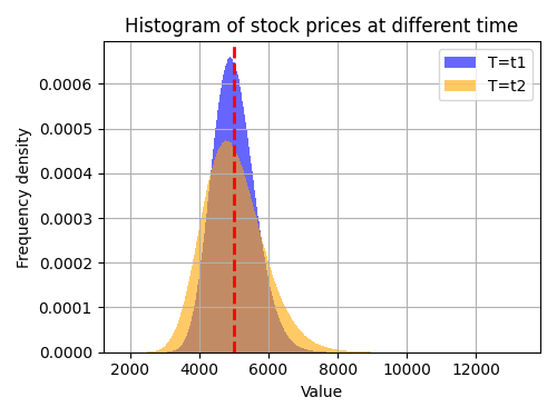
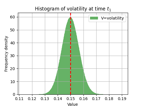
Figure 1: Histogram of stock price at time $t_{1}$ and $t_{2}$ and volatility at time $t_{1}$

Then, following the previous grid partitioning method, we extract the grid points corresponding to each dimension, transforming the data into three distributions $\mu$, $\nu$ and $\rho$. For Heston model generation, we chose $K=8\times 10^{7}$ points for simulation, implemented in the Google Colab platform, with a running time of 2 minutes 51 seconds and using approximately 9.8 GB of RAM. To make it easier to organize the notation, we present the parameters required for generating market data and calculating the reference measure during the numerical experiments, which are summarized in Table 1.

Parameters	Values/Dimensions	Explanation
$S_{0}$	5000	Initial stock price at time 0
$v_{0}$	0.15	Initial volatility at time 0
$\bar{v}$	0.15	Long-term mean of volatility
$\lambda$	1	Speed of reversion of $v_{t}$ to its long-term mean
$\eta$	0.05	Coefficient of vol of vol
$t_{1}$	0.1	First expiration date
$t_{2}$	0.2	Second expiration date
$\Delta_{t}$	0.01	Time step size
$K$	$8\times 10^{7}$	Heston model simulations number
$(\sigma_{1},\sigma_{2},\sigma_{3})$	(100,150,0.01)	Coefficient of the white noise

Table 1: Parameters and variables in Heston model

3.2.2 Experiment Results

Following the algorithm, we calculate the EMOT problem and obtain the optimized three-dimensional transition matrix. Here, we record all parameters of the algorithm in Table 2. The algorithm obtains the optimal transfer probability matrix $P^{\star}$.

Parameters	Values	Explanation
vector $x$	[3437.5, 3512.5, 3587.5,…,6362.5]	From interval [3400,6400], pick $x_{dim}=N=40$ points
vector $y$	[3235, 3305, 3375,…,6665]	From interval [3200,6700], pick $y_{dim}=M=50$ points
vector $z$	[0.138, 0.144,…,0.162]	From interval [0.135,0.165], pick $z_{dim}=5$ points
$f_{0}$	$0_{x_{dim}}$	Initial point, dimension $x_{dim}=40$
$g_{0}$	$0_{y_{dim}}$	Initial point, dimension $y_{dim}=50$
$h_{0}$	$0_{x_{dim}}$	Initial point, dimension $x_{dim}=40$
T	1000	Total iteration times
$c_{i,j,k}$	$-\log(\frac{dQ}{d\mu\otimes\nu\otimes\rho})$	Reference measure with dimensions$(40,50,5)$

Table 2: Parameters and variables in Sinkhorn’s algorithm

We need to verify whether the optimized transition probability matrix satisfies the marginal distribution and martingale conditions. From Figure 2, we can observe that the marginal distributions of matrix $P$ are consistent with $\mu$, $\nu$, and from Figure 4 they satisfy the martingale condition within a magnitude of relative error at $10^{-6}$. Also, the optimal transport matrix $P$ with fixed volatility $Z=0.15$ can be shown as in Figure 6.

From the perspective of the real market, for the given distributions $\mu$, $\nu$, and $\rho$, they do not satisfy the Heston model. Therefore, simply using SVM to calibrate the joint distribution will result in inaccurate marginal distributions. However, using the optimal joint distribution obtained from the EMOT problem not only has the same marginal distributions as the real market data but also satisfies the required martingale property for no-arbitrage. Comparing $P$ and $Q$ (see Figures 6 and 6), it can be seen a difference between the two distributions.

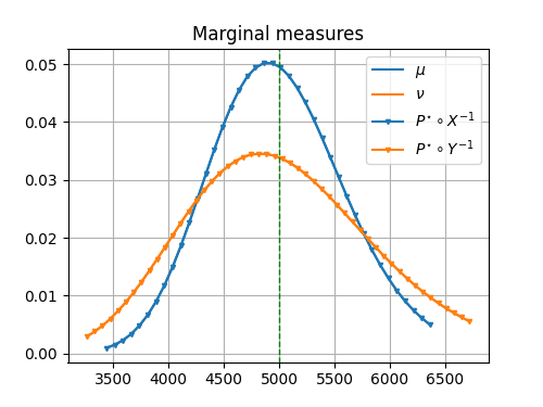
Figure 2: Lines: density function of probability measures $\mu,\nu$; Dotted lines: marginal distribution $X,Y$ of optimal transport matrix $P^{\star}$.

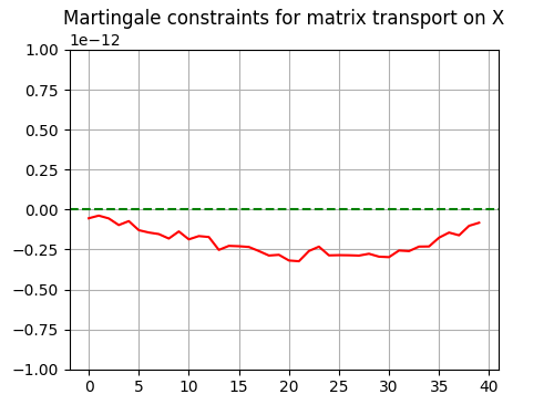
Figure 3: Martingale constraints: $\int_{\mathcal{Y},\mathcal{Z}}(y-x)d\hat{\pi}_{y,z|x}$ for different $x$.

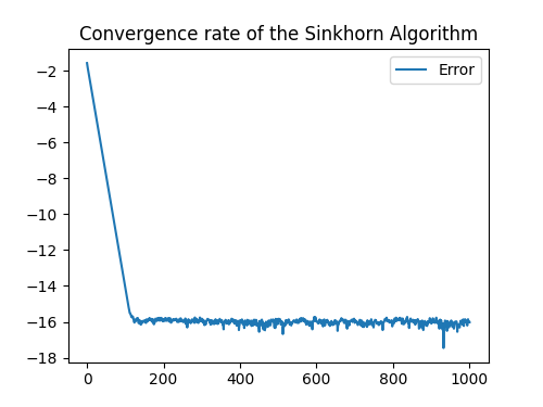
Figure 4: The convergence result: $\max_{s\in[T]}\mathcal{G}(f^{s},g^{s},h^{s})$$-\mathcal{G}(f^{t},g^{t},h^{t})$ versus the iteration step.

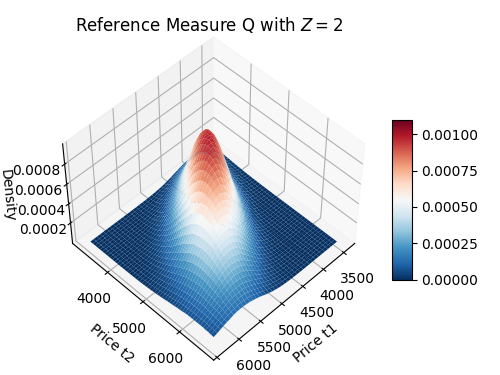
Figure 5: Reference measure $Q$ with fixed $Z=2$

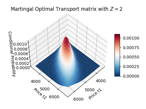
Figure 6: Martingale Optimal Transport probability matrix with fixed $Z=2$

It is noteworthy that we have recorded the latest Entropy results $H(P|Q)$ at each step during the iterative process of Sinkhorn’s algorithm, and plotted a graph of its convergence speed over time (see Figure 4). Clearly, during the 1000-step iteration process, the first 200 steps show stable convergence, and the convergence rate satisfies exponential convergence properties. And the subsequent process (200-1000 steps) is to make tiny oscillations around the optimal point, achieving the optimal solution. In the implementation process, we use the Google Colab platform to run the code, in which Sinkhorn’s algorithm is computed in about 9 seconds (110 iterations/s), which has a high running efficiency.

4 Proof of the Main Results

4.1 Uniform bound for dual functions

Proof of Proposition 2.8.

First, by Assumption 2.3 we know that $\nu$ can not be Dirac measure $\delta_{0}$ at $0$ and $\int_{\mathbb{R}}y\nu(dy)=0$, so we have $\nu((0,+\infty))>0$ and $\nu((-\infty,0))>0$. Then it can be found that there exists constants $Y^{u}$ and $Y^{d}$ such that $\nu([Y^{u},+\infty)),\nu((-\infty,Y^{d}])>0$ and $Y^{u}>Y^{d}$. We perturb the $\hat{\pi}$ from $\bar{\pi}$ as follows:

$$d\hat{\pi}(x,y,z)=\left\{\begin{array}[]{l}d\bar{\pi}(x,y,z)+\delta\mu((-\infty,0))\nu((-\infty,Y^{d}])d\mu\otimes\nu\otimes\rho,\text{\quad for\ \ }x\geq 0\ \text{and}\ y\geq Y^{u};\\ d\bar{\pi}(x,y,z)-\delta\mu([0,+\infty))\nu((-\infty,Y^{d}])d\mu\otimes\nu\otimes\rho,\text{\quad for\ \ }x<0\ \text{and}\ y\geq Y^{u};\\ d\bar{\pi}(x,y,z)-\delta\mu((-\infty,0))\nu([Y^{u},+\infty))d\mu\otimes\nu\otimes\rho,\text{\quad for\ \ }x\geq 0\ \text{and}\ y\leq Y^{d};\\ d\bar{\pi}(x,y,z)+\delta\mu([0,+\infty))\nu([Y^{u},+\infty))d\mu\otimes\nu\otimes\rho,\text{\quad for\ \ }x<0\ \text{and}\ y\leq Y^{d};\\ d\bar{\pi}(x,y,z),\quad\text{otherwise};\end{array}\right.$$

where $\delta$ is a positive constant such that

$$\delta:=\frac{1}{2\big{(}\mu((-\infty,0))\vee\mu([0,+\infty))\big{)}\cdot\big{(}\nu((-\infty,Y^{d}])\vee\nu([Y^{u},+\infty))\big{)}}\cdot\exp(-|p|_{L^{\infty}(\mu\otimes\nu\otimes\rho)}).$$

It is easy to check from construction that

$$\frac{1}{2}\cdot\frac{d\bar{\pi}}{d\mu\otimes\nu\otimes\rho}\leq\frac{d\hat{\pi}}{d\mu\otimes\nu\otimes\rho}\leq\frac{3}{2}\cdot\frac{d\bar{\pi}}{d\mu\otimes\nu\otimes\rho}.$$ (4.1)

We can show $\hat{\pi}\in\Pi(\mu,\nu)$, using the equalities

$$\int_{\mathcal{Y}\times\mathcal{Z}} \hat{\pi}(dx,dy,dz)-\int_{\mathcal{Y}\times\mathcal{Z}}\bar{\pi}(dx,dy,dz)$$

$$=\delta\Big{(}\int_{y\geq Y^{u}}\mu((-\infty,0))\nu((-\infty,Y^{d}])d\nu-\int_{y\leq Y^{d}}\mu((-\infty,0))\nu([Y^{u},+\infty))d\nu\Big{)}\mu(dx)=0,\quad\mbox{for $x\geq 0$},$$

$$\int_{\mathcal{X}\times\mathcal{Z}} \hat{\pi}(dx,dy,dz)-\int_{\mathcal{X}\times\mathcal{Z}}\bar{\pi}(dx,dy,dz)$$

$$=\delta\Big{(}\int_{x\geq 0}\mu((-\infty,0))\nu((-\infty,Y^{d}])d\mu-\int_{x<0}\mu([0,+\infty))\nu((-\infty,Y^{d}])d\mu\Big{)}\nu(dy)=0,\quad\mbox{for $y>Y^{u}$}.$$

By a similar computation, the result can also be shown for the case $x<0$ and $y\leq Y^{d}$, and therefore we get $\hat{\pi}\in\Pi(\mu,\nu)$. The conditional increment $\int_{\mathcal{Y},\mathcal{Z}}(y-x)d\hat{\pi}_{y,z|x}$ for $x\geq 0$ can be calculated by noticing the difference

$$\int_{\mathcal{Y}}(y -x)d\hat{\pi}_{y,z|x}-\int_{\mathcal{Y}}(y-x)d\bar{\pi}_{y,z|x}$$

$$=\delta\int_{y\geq Y^{u}}(y-x)\mu((-\infty,0))\nu((-\infty,Y^{d}])\nu(dy)-\delta\int_{\tilde{y}\leq Y^{d}}(\tilde{y}-x)\mu((-\infty,0))\nu([Y^{u},+\infty))\nu(d\tilde{y})$$

$$=\delta\int_{y\geq Y^{u}}y\mu((-\infty,0))\nu((-\infty,Y^{d}])\nu(dy)-\delta\int_{\tilde{y}\leq Y^{d}}\tilde{y}\mu((-\infty,0))\nu([Y^{u},+\infty))\nu(d\tilde{y})$$

$$\geq\delta(Y^{u}-Y^{d})\mu((-\infty,0))\big{(}\nu([Y^{u},+\infty))\wedge\nu((-\infty,Y^{d}])\big{)},$$

where we use the martingale property for $\bar{\pi}$ to yield the subtractor on the left cancels in the second equality. Similarly, we can deduce the inequality for $x<0$, and the conditional increment for $\hat{\pi}$ can be computed and summarized to be

$$\int_{\mathcal{Y}}(y-x)d\hat{\pi}_{y|x}\left\{\begin{array}[]{l}\geq\ \ \delta(Y^{u}-Y^{d})\mu((-\infty,0))\big{(}\nu([Y^{u},+\infty))\wedge\nu((-\infty,Y^{d}])\big{)},\text{\quad for\ }x\geq 0;\\ \leq-\delta(Y^{u}-Y^{d})\mu([0,+\infty))\big{(}\nu([Y^{u},+\infty))\wedge\nu((-\infty,Y^{d}])\big{)},\text{\quad for\ }x<0;\\ \end{array}\right.$$

As a consequence, it is possible for us to find a constant $\epsilon_{p}$ to satisfy the required condition (2.8). Furthermore, the relative entropy is finite. It follows from inequality (4.1), we have $d\hat{\pi}/d\bar{\pi}\in[1/2,3/2]$, so that

$$H(\hat{\pi}|Q)\leq\int\Big{|}\log\frac{d\hat{\pi}}{dQ}\Big{|}d\bar{\pi}\leq\int\Big{|}\log\frac{d\bar{\pi}}{dQ}\Big{|}d\hat{\pi}+\log 2\leq\frac{3}{2}\int\Big{|}\log\frac{d\bar{\pi}}{dQ}\Big{|}d\bar{\pi}+\log 2,$$

and for the right-hand side, we finally have

$$\int\Big{|}\log\frac{d\bar{\pi}}{dQ}\Big{|}d\bar{\pi} =H(\bar{\pi}|Q)+2\int\Big{(}\log\frac{d\bar{\pi}}{dQ}\Big{)}^{-}d\bar{\pi}\leq H(\bar{\pi}|Q)+2e^{-1}.$$

∎

In the following, we are going to provide a uniform $L^{1}(\mu\otimes\nu\otimes\rho)$ bound for the dual coefficients and then derive a uniform $L^{\infty}(\mu\otimes\nu\otimes\rho)$ bound. Note that the estimates are stable under the invariant transforms (2.7).

Proposition 4.1.

Under Assumptions 2.2, 2.3 and 2.6, through Sinkhorn’s iterations, the functions $(\tilde{f}^{n},\tilde{g}^{n},\tilde{h}^{n})_{n\geq 1}$ satisfy the uniform $L^{1}$-estimate:

$$\sup_{n\geq 1}|\tilde{h}^{n}-\tilde{h}^{n}(0)|_{L^{1}(\mu)}<+\infty,$$

$$\sup_{n\geq 1}\int\big{|}\tilde{f}^{n}(x)-\tilde{f}^{n}(0)-\tilde{h}^{n}(0)x\big{|}\mu(dx)<+\infty,$$

$$\sup_{n\geq 1}\int\big{|}\tilde{g}^{n}(y)+\tilde{f}^{n}(0)+\tilde{h}^{n}(0)y\big{|}\nu(dy)<+\infty.$$

In addition, we have the following uniform point-wise upper bound for the value $\tilde{f}^{n}(x)-\tilde{f}^{n}(0)-\tilde{h}^{n}(0)x$:

$$\sup_{n\geq 1}\tilde{f}^{n}(x)-\tilde{f}^{n}(0)-\tilde{h}^{n}(0)x\leq L_{c}|x|.$$ (4.2)

Proof.

For any $x,x^{\prime}\in\mathcal{X}_{0}$, we derive the first estimation

$$\log\int_{\mathcal{Y}\times\mathcal{Z}} \exp(-c(x,y,z)-g^{n}(y)-\tilde{h}^{n+1}(x)(y-x))\nu(dy)\rho(dz)$$ (4.3)

$$\quad\quad\quad\quad\quad-\log\int_{\mathcal{Y}\times\mathcal{Z}}\exp(-c(x^{\prime},y,z)-g^{n}(y)-\tilde{h}^{n+1}(x^{\prime})(y-x^{\prime}))\nu(dy)\rho(dz)$$

$$\geq-\int_{\mathcal{Y}\times\mathcal{Z}}(c(x,y,z)-c(x^{\prime},y,z))\pi_{y,z|x^{\prime}}(dy,dz)-\int_{\mathcal{Y}\times\mathcal{Z}}\big{[}\tilde{h}^{n+1}(x)(y-x)-\tilde{h}^{n+1}(x^{\prime})(y-x^{\prime})\big{]}\pi_{y,z|x^{\prime}}(dy,dz)$$

$$\geq-L_{c}|x^{\prime}-x|-\tilde{h}^{n+1}(x)(x^{\prime}-x),$$

where the second term of the last inequality simplifies due to the martingale property of $\pi_{y|x^{\prime}}=\pi_{y|x^{\prime}}(\cdot,g^{n},\tilde{h}^{n+1})$. We omitted the first variable in expression $\pi_{y|x^{\prime}}(\cdot,g^{n},\tilde{h}^{n+1})$ because this conditional probability measure does not depend on the first variable $f$. By exchanging the roles of $x$ and $x^{\prime}$ and summing up the two inequalities, it comes to

$$(x^{\prime}-x)\Big{(}\tilde{h}^{n+1}(x^{\prime})-\tilde{h}^{n+1}(x)\Big{)}\leq 2L_{c}|x-x^{\prime}|,\quad\mbox{and therefore}\quad\big{(}\tilde{h}^{n+1}(x^{\prime})-\tilde{h}^{n+1}(x)\big{)}\textrm{sgn}(x^{\prime}-x)\leq 2L_{c}.$$ (4.4)

Taking $x^{\prime}=0$, we obtain $\tilde{h}^{n+1}(x)-\tilde{h}^{n+1}(0)\leq 2L_{c}$ for $x\geq 0$ and $\tilde{h}^{n+1}(x)-\tilde{h}^{n+1}(0)\geq-2L_{c}$ for $x<0$. Using the probability measure $\hat{\pi}$ constructed in Proposition 2.8, we know

$$H(\hat{\pi}|Q)+\int_{\mathcal{X}}\tilde{h}^{n+1}(x)\int_{\mathcal{Y}\times\mathcal{Z}}(y-x)d\hat{\pi}\geq\inf_{\pi\in\Pi(\mu,\nu)}H(\pi|Q)+\int_{\mathcal{X}}\tilde{h}^{n+1}(x)\int_{\mathcal{Y}\times\mathcal{Z}}(y-x)d\pi\geq\mathcal{G}(\tilde{f}^{n+1},g^{n},\tilde{h}^{n+1}),$$ (4.5)

where the last inequality follows from the duality. In addition, $\mathcal{G}(\tilde{f}^{n+1},g^{n},\tilde{h}^{n+1})\geq\mathcal{G}(f^{0},g^{0},h^{0})$ for all $n$. Further, by the compactness of support for $\mu$ and $\nu$, there exists $C_{0}>0$ such that

$$\int_{\mathcal{X}}\Big{(}\tilde{h}^{n+1}(x)-\tilde{h}^{n+1}(0)-2L_{c}\textrm{sgn}(x)\Big{)}\int_{\mathcal{Y}\times\mathcal{Z}}(y-x)\hat{\pi}_{y,z|x}(dy)\hat{\pi}_{x}(dx)\geq-C_{0}.$$ (4.6)

Recall that $\hat{\pi}_{x}=\mu$ and that the integrand on the left is non-positive thanks to (4.4). Therefore,

$$\epsilon_{p}\int_{\mathcal{X}}\Big{|}\tilde{h}^{n+1}(x) -\tilde{h}^{n+1}(0)-2L_{c}\textrm{sgn}(x)\Big{|}\mu(dx)$$

$$\leq\int_{\mathcal{X}}\big{|}\tilde{h}^{n+1}(x)-\tilde{h}^{n+1}(0)-2L_{c}\textrm{sgn}(x)\big{|}\Big{|}\int_{\mathcal{Y}\times\mathcal{Z}}(y-x)\hat{\pi}_{y,z|x}(dy)\Big{|}\mu(dx)\leq C_{0},$$

so that it can be deduced that $|\tilde{h}^{n+1}-\tilde{h}^{n+1}(0)|$ is uniformly bounded in $L^{1}(\mu)$.

Next, we consider the first-order equality of $\tilde{f}^{n+1}$, which writes,

$$\log\int_{\mathcal{Y}\times\mathcal{Z}}\exp(-c(x,y,z)-g^{n}(y)-\tilde{h}^{n+1}(x)y)(\nu\otimes\rho)(dy,dz)=\tilde{f}^{n+1}(x)-x\tilde{h}^{n+1}(x).$$

Together with the convexity inequality $\exp(x)-\exp(y)\geq\exp(y)(x-y)$, we estimate:

$$\tilde{f}^{n+1}(x) -\tilde{f}^{n+1}(0)-\tilde{h}^{n+1}(0)x=\tilde{f}^{n+1}(x)-\tilde{h}^{n+1}(x)x-\tilde{f}^{n+1}(0)+\big{(}\tilde{h}^{n+1}(x)-\tilde{h}^{n+1}(0)\big{)}x$$ (4.7)

$$\geq\int_{\mathcal{Y}\times\mathcal{Z}}\Big{(}c(0,y,z)-c(x,y,z)-\big{(}\tilde{h}^{n+1}(x)-\tilde{h}^{n+1}(0)\big{)}y\Big{)}\pi_{y,z|0}(dy)+\big{(}\tilde{h}^{n+1}(x)-\tilde{h}^{n+1}(0)\big{)}x$$

$$\geq-L_{c}|x|+\big{(}\tilde{h}^{n+1}(x)-\tilde{h}^{n+1}(0)\big{)}x.$$

On the other hand, using the inequality $\exp(x)-\exp(y)\leq\exp(x)(x-y)$, we obtain

$$\tilde{f}^{n+1}(x) -\tilde{f}^{n+1}(0)-\tilde{h}^{n+1}(0)x$$

$$\leq\int_{\mathcal{Y}\times\mathcal{Z}}\Big{(}c(0,y,z)-c(x,y,z)-\big{(}\tilde{h}^{n+1}(x)-\tilde{h}^{n+1}(0)\big{)}y\Big{)}\pi_{y,z|x}(dy)+\big{(}\tilde{h}^{n+1}(x)-\tilde{h}^{n+1}(0)\big{)}x$$

$$\leq L_{c}|x|-\big{(}\tilde{h}^{n+1}(x)-\tilde{h}^{n+1}(0)\big{)}x+\big{(}\tilde{h}^{n+1}(x)-\tilde{h}^{n+1}(0)\big{)}x=L_{c}|x|.$$

Therefore, $\tilde{f}^{n+1}-\tilde{f}^{n+1}(0)-\tilde{h}^{n+1}(0)x$ is uniformly bounded in $L^{1}(\mu)$ norm.

Finally for $\tilde{g}^{n+1}$, again by the convexity of $z\mapsto\exp(z)$ we get:

$$0=\int_{\mathcal{X}\times\mathcal{Z}} \big{(}\exp(-c(x,y,z)-\tilde{f}^{n+1}(x)-\tilde{g}^{n+1}(y)-\tilde{h}^{n+1}(x)(y-x))-\exp(-p(x,y,z))\big{)}d(\mu\otimes\rho)$$

$$\geq\int_{\mathcal{X}\times\mathcal{Z}}\exp(-p(x,y,z))\big{(}p(x,y,z)-c(x,y,z)-\tilde{f}^{n+1}(x)-\tilde{g}^{n+1}(y)-\tilde{h}^{n+1}(x)(y-x)\big{)}d(\mu\otimes\rho)$$

$$\geq-|p|_{L^{\infty}}-|c|_{L^{\infty}}-\tilde{g}^{n+1}(y)-\tilde{f}^{n+1}(0)-\tilde{h}^{n+1}(0)y-\int_{\mathcal{X}}\big{(}\tilde{f}^{n+1}(x)-\tilde{f}^{n+1}(0)+\tilde{h}^{n+1}(0)x\big{)}d\mu$$

$$\quad\quad\quad\quad\quad\quad\quad\quad\quad\quad\quad\quad-(|\mathcal{X}|_{\infty}+|\mathcal{Y}|_{\infty})|\tilde{h}^{n+1}-\tilde{h}^{n+1}(0)|_{L^{1}(\mu)},$$

where the probability measure $\bar{\pi}=\exp(-p(x,y,z))d\mu\otimes\nu\otimes\rho\in\mathcal{M}(\mu,\nu)$. Recalling that the function $\mathcal{G}(\tilde{f}^{n+1},\tilde{g}^{n+1},\tilde{h}^{n+1})=-1-\int_{\mathcal{X}}\tilde{f}^{n+1}d\mu-\int_{\mathcal{Y}}\tilde{g}^{n+1}d\nu$, the inequality above implies a lower bound for the quantity: $\tilde{g}^{n+1}(y)+\tilde{f}^{n+1}(0)+\tilde{h}^{n+1}(0)\cdot y\geq-C_{1}$. It follows from the optimality condition for $\tilde{g}^{n+1}$ that

$$\int_{\mathcal{Y}\times\mathcal{Z}}(\tilde{g}^{n+1} +\tilde{f}^{n+1}(0)+\tilde{h}^{n+1}(0)y+C_{1})d(\nu\otimes\rho)$$

$$=C_{1}+1-1-\int_{\mathcal{X}}\tilde{f}^{n+1}d\mu-\int_{\mathcal{Y}}\tilde{g}^{n+1}d\nu+\int_{\mathcal{X}}\big{(}\tilde{f}^{n+1}-\tilde{f}^{n+1}(0)-\tilde{h}^{n+1}(0)x\big{)}d\mu$$

$$=C_{1}+1-\mathcal{G}(\tilde{f}^{n+1},\tilde{g}^{n+1},\tilde{h}^{n+1})-\int_{\mathcal{X}}\big{(}\tilde{f}^{n+1}-\tilde{f}^{n+1}(0)-\tilde{h}^{n+1}(0)x\big{)}d\mu.$$

The integrand on the left is positive, so we see that $\tilde{g}^{n+1}+\tilde{f}^{n+1}(0)+\tilde{h}^{n+1}(0)y$ has a uniform bound in $L^{1}(\nu)$, hence the proof completes. ∎

Proof of Theorem 2.9.

Given the previous uniform $L^{1}$-bound of the dual coefficients $(f^{n+1},g^{n+1},h^{n+1})_{n}$ by Proposition 4.1 and (2.6), we are ready to show a uniform $L^{\infty}$-bound for them, using the probability measure $\hat{\pi}$ given in Proposition 2.8. We know that for $(\tilde{f}^{n+1},g^{n},\tilde{h}^{n+1})$, the induced probability measure satisfies the martingale property and the $\mathcal{X}$-marginal distribution satisfies $\pi_{x}=\mu$. Recall the probability constructed in Proposition 2.8: $\hat{\pi}=\exp(-\hat{p}(x,y,z))d\mu\otimes\nu\otimes\rho\in\Pi(\mu,\nu)$. Since $\pi_{x}=\mu=\hat{\pi}_{x}$, we have

$$0=\int_{\mathcal{Y}\times\mathcal{Z}} \big{(}\exp(-c(x,y,z)-\tilde{f}^{n+1}(x)-g^{n}(y)-\tilde{h}^{n+1}(x)(y-x))-\exp(-\hat{p}(x,y,z))\big{)}d(\nu\otimes\rho)$$

$$\geq\int_{\mathcal{Y}\times\mathcal{Z}}\exp(-\hat{p}(x,y,z))\big{(}p(x,y,z)-c(x,y,z)-\tilde{f}^{n+1}(x)-g^{n}(y)-\tilde{h}^{n+1}(x)(y-x)\big{)}d(\nu\otimes\rho)$$

$$\geq-|\hat{p}|_{\infty}-|c|_{\infty}-\int_{\mathcal{Y}\times\mathcal{Z}}\tilde{f}^{n+1}(x)+g^{n}(y)+\tilde{h}^{n+1}(x)(y-x)d\hat{\pi}_{y,z|x}(x,dy,dz)$$

$$\geq-|\hat{p}|_{\infty}-|c|_{\infty}-\int_{\mathcal{Y}\times\mathcal{Z}}\tilde{f}^{n+1}(x)+g^{n}(y)+\tilde{h}^{n+1}(0)(y-x)d\hat{\pi}_{y,z|x}(x,dy,dz)$$

$$\quad\quad\quad\quad\quad\quad\quad\quad\quad\quad\quad+\int_{\mathcal{Y}\times Z}\big{(}\tilde{h}^{n+1}(x)-\tilde{h}^{n+1}(0)\big{)}(y-x)d\hat{\pi}_{y,z|x}(x,dy,dz).$$

By applying the uniform upper bound in (4.2), we obtain

$$\big{(}\tilde{h}^{n+1} (x)-\tilde{h}^{n+1}(0)\big{)}\int_{\mathcal{Y}\times\mathcal{Z}}(y-x)d\hat{\pi}_{y,z|x}(x,dy,dz)$$ (4.8)

$$\quad\geq-|\hat{p}|_{\infty}-|c|_{\infty}-|(\tilde{f}^{n+1}-\tilde{f}^{n+1}(0)-\tilde{h}^{n+1}(x)x)^{+}|_{L^{\infty}}-|\tilde{g}^{n+1}+\tilde{f}^{n+1}(0)+\tilde{h}^{n+1}(0)y|_{L^{1}(\nu)}=:-C_{2}.$$

Therefore, for $x\geq 0$ it holds $\tilde{h}^{n+1}(x)-\tilde{h}^{n+1}(0)\geq-C_{2}/\epsilon_{p}$ for $\epsilon_{p}$ given in Proposition 2.8. And similarly for $x<0$, it has $\tilde{h}^{n+1}(x)-\tilde{h}^{n+1}(0)\leq C_{2}/\epsilon_{p}$. Together with the bound in (4.4) we arrive at a uniform $L^{\infty}(\mu)$-bound for $\tilde{h}^{n+1}(x)-\tilde{h}^{n+1}(0)$.

Next, we are going to deduce the uniform $L^{\infty}$-bound for $\tilde{f}^{n+1}-\tilde{f}^{n+1}(0)-\tilde{h}^{n+1}(0)x$ and $\tilde{g}^{n+1}+\tilde{f}^{n+1}(0)+\tilde{h}^{n+1}(0)y$. For the former we recall (4.7) to obtain its uniform $L^{\infty}(\mu)$-bound, and for the latter we write

$$\tilde{g}^{n+1}(y) +\tilde{f}^{n+1}(0)+\tilde{h}^{n+1}(0)y$$

$$=\log\int_{\mathcal{X}\times\mathcal{Z}}\exp\Big{(}-c(x,y,z)-\big{(}\tilde{f}^{n+1}(x)-\tilde{f}^{n+1}(0)-\tilde{h}^{n+1}(0)x\big{)}-\big{(}\tilde{h}^{n+1}(x)-\tilde{h}^{n+1}(0)\big{)}(y-x)\Big{)}d(\mu\otimes\rho),$$

where the uniform $L^{\infty}(\mu)$-bounds of $\tilde{f}^{n+1}-\tilde{f}^{n+1}(0)-\tilde{h}^{n+1}(0)x$ and $\tilde{h}^{n+1}-\tilde{h}^{n+1}(0)$ are used to get the desired uniform $L^{\infty}(\nu)$-bound. ∎

Remark 4.2.

In our problem, the construction of $\hat{\pi}$ is crucial because it implies the bounds in (4.4) and (4.8). For the case of high dimensional EMOT problem when $\mathcal{X},\mathcal{Y}=\mathbb{R}^{d}$, in order to mimic the argument of the Theorem 2.9, we need but failed to construct a $\hat{\pi}\sim\mu\otimes\nu\otimes\rho$ such that $H(\hat{\pi}|\mu\otimes\nu\otimes\rho)<+\infty$ and $\int_{\mathcal{Y}\times\mathcal{Z}}(y-x)\hat{\pi}_{y,z|x}(dy)=\epsilon(x)x/|x|$ for $x\in\mathcal{X}$, $\mu$-a.s, where $\epsilon(x)$ has a uniform positive lower bound $\epsilon_{0}$, i.e., $\epsilon(x)\geq\epsilon_{0}$.

4.2 Exponential convergence

The proof of Theorem 2.10 begins with leveraging the uniform bounds of dual coefficients proved in Theorem 2.9, namely, $|f^{n}(x)|_{L^{\infty}(\mu)}\leq C_{f},|g^{n}(x)|_{L^{\infty}(\nu)}\leq C_{g}$ and $|h^{n}(x)|_{L^{\infty}(\mu)}\leq C_{h}$, so as to establish the exponential convergence of the sequence $\big{(}\mathcal{G}(f^{n},g^{n},h^{n})\big{)}_{n}$. As a result, the sequence of functions $(f^{n},g^{n},h^{n})_{n}$ is uniformly convergent, and it converges to a triple $(f^{*},g^{*},h^{*})\in(L^{\infty}(\mu)\times L^{\infty}(\nu)\times L^{\infty}(\mu))$. Subsequently, we verify the first-order optimality condition for the primal problem (2.1), confirming that the triple $(f^{*},g^{*},h^{*})$ induces a probability measure, which solves the original problem (2.1). Eventually it establishes the absence of a primal-dual gap in this duality correlation.

Lemma 4.3.

Under Assumptions 2.2, 2.3 and 2.6, for any $n\in\mathbb{N}^{+}$ we define the set $\mathcal{I}^{n}$:

$$\mathcal{I}^{n}:=\{(f^{n},g^{n},h^{n}),(f^{n},g^{n},\tilde{h}^{n+1}),(\tilde{f}^{n+1},g^{n},\tilde{h}^{n+1}),(\tilde{f}^{n+1},\tilde{g}^{n+1},\tilde{h}^{n+1})\}.$$

There exist positive constants $C_{f}^{\prime}\geq C_{f},C_{g}^{\prime}\geq C_{g},C_{h}^{\prime}=C_{h}$ such that for any $n\in\mathbb{N}^{+}$ and any $(f,g,h)\in\mathcal{I}^{n}$

$$|h(x) -h(0)|_{L^{\infty}(\mu)}\leq C_{h}^{\prime},\quad|f(x)-f(0)-h(0)x|_{L^{\infty}(\mu)}\leq C_{f}^{\prime}$$

$$\text{and}\quad|g(y)+f(0)+h(0)y|_{L^{\infty}(\nu)}\leq C_{g}^{\prime}.$$

Proof.

The uniform bound for the first and the last triple in $\mathcal{I}^{n}$ have already been given in Theorem 2.9. As for the second triple $(f^{n},g^{n},\tilde{h}^{n+1})$, due to the uniform-in-$n$ $L^{\infty}(\nu)$-boundedness of $(g^{n})_{n}$ we can find a uniform constant $c_{h}>0$ such that $|\tilde{h}^{n+1}(0)|\leq c_{h}$ by Proposition 2.7. Together with Theorem 2.9, the following estimates hold,

$$|\tilde{h}^{n+1}(x) -\tilde{h}^{n+1}(0)|_{L^{\infty}(\mu)}\leq C_{h},\quad|f^{n}(x)-f^{n}(0)-\tilde{h}^{n+1}(0)x|_{L^{\infty}(\nu)}\leq C_{f}+c_{h}|\mathcal{X}|$$

$$\text{and}\quad|g^{n}(y)+f^{n}(0)+\tilde{h}^{n+1}(0)y|_{L^{\infty}(\mu\otimes\nu)}\leq C_{g}+c_{h}|\mathcal{Y}|,$$

where we recall $f^{n}(0)=0$ and $|f^{n}|_{L^{\infty}(\mu)}\leq C_{f},|g^{n}|_{L^{\infty}(\nu)}\leq C_{g}$. Next, we consider the triple $(\tilde{f}^{n+1},g^{n},\tilde{h}^{n+1})$. It can be derived from the definition of $\tilde{f}^{n+1}(0)$ (see (2.5)) that $|\tilde{f}^{n+1}(0)|\leq|c|_{L^{\infty}}+C_{g}+c_{h}|\mathcal{Y}|$. And it follows again from Theorem 2.9 that

$$|\tilde{f}^{n+1}(x) -\tilde{f}^{n+1}(0)-\tilde{h}^{n+1}(0)x|_{L^{\infty}(\nu)}\leq C_{f},$$

$$\text{and}\quad|g^{n}(y)+\tilde{f}^{n+1}(0)+\tilde{h}^{n+1}(0)y|_{L^{\infty}(\mu\otimes\nu)}\leq 2C_{g}+2c_{h}|\mathcal{Y}|+|c|_{L^{\infty}}.$$

Finally, we choose $C_{f}^{\prime}:=C_{f}+c_{h}|\mathcal{X}|,C_{g}^{\prime}:=2C_{g}+2c_{h}|\mathcal{Y}|+|c|_{L^{\infty}}$ and $C_{h}^{\prime}:=C_{h}$ so that the desired unified estimates hold true. ∎

The proof of exponential convergence shares some similarities with [7], which studies Sinkhorn’s algorithm for entropic optimal transport without the martingale constraint. However, the martingale constraint and the corresponding dual term $h(x)(y-x)$ bring the major difficulties.

Define $C_{0}:=C_{f}^{\prime}+C_{g}^{\prime}+C_{h}^{\prime}(|\mathcal{X}|+|\mathcal{Y}|)+|c|_{L^{\infty}}$. Then we have

$$|c(x,y,z)+f(x)+g(y)+h(x)(y-x)|\leq C_{0}.$$

Besides, denoting $\kappa:=\exp(-C_{0})$, the density of probability measure $\pi(f,g,h)$ with respect to base measure $\mu\otimes\nu\otimes\rho$ can be bounded from both sides, that is,

$$\kappa\leq\frac{d\pi(f,g,h)}{d(\mu\otimes\nu\otimes\rho)}=\exp(-c(x,y,z)-f(x)-g(y)-h(x)(y-x))\leq\kappa^{-1},$$ (4.9)

for arbitrary $(f,g,h)\in\mathcal{I}^{n}$. We define the set $\mathcal{S}$ of functions:

$$\mathcal{S}:=\{(f,g,h):(f,g,h) \in(L^{\infty}(\mu)\times L^{\infty}(\nu)\times L^{\infty}(\mu)),|f(x)-f(0)-h(0)x|\leq C_{f}^{\prime},$$

$$\qquad|g(y)+f(0)+h(0)y|\leq C_{g}^{\prime},|h(x)-h(0)|\leq C_{h}^{\prime},\quad\text{ for }x\ \mu\text{-}a.s.,y\ \nu\text{-}a.s.\}.$$

Lemma 4.3 yields that for any $n\in\mathbb{N}^{+}$, the set $\mathcal{I}^{n}\subset\mathcal{S}$.

For a function $\mathcal{F}:(L^{\infty}(\mu)\times L^{\infty}(\nu)\times L^{\infty}(\mu))\to\mathbb{R}$, let us define the linear functional derivatives $\frac{\delta\mathcal{F}}{\delta f}:L^{\infty}(\mu)\times\mathbb{R}^{3}\to\mathbb{R}^{3},\frac{\delta\mathcal{F}}{\delta g}:L^{\infty}(\nu)\times\mathbb{R}^{3}\to\mathbb{R}^{3}$, and $\frac{\delta\mathcal{F}}{\delta h}:L^{\infty}(\mu)\times\mathbb{R}^{3}\to\mathbb{R}^{3}$ such that for any $(f,g,h),(f^{\prime},g^{\prime},h^{\prime})\in(L^{\infty}(\mu)\times L^{\infty}(\nu)\times L^{\infty}(\mu))$, it holds:

$$\mathcal{F}(f^{\prime},g^{\prime},h^{\prime})-\mathcal{F}(f,g,h)=\int_{0}^{1}\Big{[}\int_{\mathbb{R}}\frac{\delta\mathcal{F}}{\delta f}\big{(}tf^{\prime}+(1-t)f\big{)}(x)(f^{\prime}-f)(x)\mu(dx)$$

$$+\int_{\mathbb{R}}\frac{\delta\mathcal{F}}{\delta g}\big{(}tg^{\prime}+(1-t)g\big{)}(y)(g^{\prime}-g)(y)\nu(dy)+\int_{\mathbb{R}}\frac{\delta\mathcal{F}}{\delta h}\big{(}th^{\prime}+(1-t)h\big{)}(x)(h^{\prime}-h)(x)\mu(dx)\Big{]}dt.$$

Lemma 4.4.

Under Assumption 2.2, for any $(f,g,h)$, $(\tilde{f},\tilde{g},\tilde{h})\in\mathcal{S}$, the function derivative of $\mathcal{G}(f,g,h)$ satisfies the following estimations:

$$\Bigg{|}\frac{\delta\mathcal{G}}{\delta f}(\tilde{f},\tilde{g},\tilde{h})(x)-\frac{\delta\mathcal{G}}{\delta f}(f,g,h)(x)\Bigg{|}_{L^{2}(\mu)}^{2}\leq M_{f}^{2}\big{|}\tilde{f}-f+\tilde{g}-g+(\tilde{h}-h)(y-x)\big{|}_{L^{2}(\mu\otimes\nu)}^{2},\quad$$ (4.10)

$$\Bigg{|}\frac{\delta\mathcal{G}}{\delta g}(\tilde{f},\tilde{g},\tilde{h})(y)-\frac{\delta\mathcal{G}}{\delta g}(f,g,h)(y)\Bigg{|}_{L^{2}(\nu)}^{2}\leq M_{g}^{2}\big{|}\tilde{f}-f+\tilde{g}-g+(\tilde{h}-h)(y-x)\big{|}_{L^{2}(\mu\otimes\nu)}^{2},$$

$$\Bigg{|}\frac{\delta\mathcal{G}}{\delta h}(\tilde{f},\tilde{g},\tilde{h})(x)-\frac{\delta\mathcal{G}}{\delta h}(f,g,h)(x)\Bigg{|}_{L^{2}(\mu)}^{2}\leq M_{h}^{2}\big{|}\tilde{f}-f+\tilde{g}-g+(\tilde{h}-h)(y-x)\big{|}_{L^{2}(\mu\otimes\nu)}^{2},$$

where $M_{f}=M_{g}=\kappa^{-1}$, and $M_{h}=\kappa^{-1}(|\mathcal{X}|+|\mathcal{Y}|)$.

Proof.

Let us consider the linear functional derivative of $\mathcal{G}$ with respect to $(f,g,h)$ under measure $\mu$ and $\nu$:

$$\frac{\delta\mathcal{G}}{\delta f}(f,g,h)(x)=\int_{\mathcal{Y}\times\mathcal{Z}}{\exp\big{(}-c(x,y,z)-f(x)-g(y)-h(x)(y-x)\big{)}(\nu\otimes\rho)(dy,dz)}-1,$$ (4.11)

$$\frac{\delta\mathcal{G}}{\delta g}(f,g,h)(y)=\int_{\mathcal{X}\times\mathcal{Z}}{\exp\big{(}-c(x,y,z)-f(x)-g(y)-h(x)(y-x)\big{)}(\nu\otimes\rho)(dx,dz)}-1,$$

$$\frac{\delta\mathcal{G}}{\delta h}(f,g,h)(x)=\int_{\mathcal{Y}\times\mathcal{Z}}{(y-x)\exp\big{(}-c(x,y,z)-f(x)-g(y)-h(x)(y-x)\big{)}(\nu\otimes\rho)(dy,dz)},$$

defined for $x\ \mu\text{-}a.s.,y\ \nu\text{-}a.s.$. For inequalities (4.10), we prove the third one as an example and the rest can be shown similarly. From the compactness of the support for measures $\mu$ and $\nu$ and the basic inequality

$$|\exp(x)-\exp(y)|\leq\exp(x\vee y)|x-y|,$$

for any $x,y\in\mathbb{R}$, we have

$$\big{|}\exp(-c(x,y,z)- \tilde{f}(x)-\tilde{g}(y)-\tilde{h}(x)(y-x))-\exp(-c(x,y,z)-f(x)-g(y)-h(x)(y-x))\big{|}$$

$$\leq\kappa^{-1}|\tilde{f}(x)-f(x)+\tilde{g}(y)-g(y)+(\tilde{h}-h)(x)(y-x)|,\quad\text{for\ }x\ \mu\text{-}a.s..$$

It follows that

$$\int_{\mathcal{Y}\times\mathcal{Z}}(y-x) \Big{(}\exp\big{(}-c(x,y,z)-\tilde{f}(x)-\tilde{g}(y)-\tilde{h}(x)(y-x)\big{)}$$

$$\quad\quad\quad\quad\quad\quad\quad\quad\quad\quad-\exp\big{(}-c(x,y,z)-f(x)-g(y)-h(x)(y-x)\big{)}\Big{)}(\nu\otimes\rho)(dy,dz)$$

$$\leq(|\mathcal{X}|+|\mathcal{Y}|)\kappa^{-1}\int_{\mathcal{Y}}\big{|}\tilde{f}(x)-f(x)+\tilde{g}(y)-g(y)+(\tilde{h}-h)(x)(y-x)\big{|}\nu(dy).$$

Together with (4.11), we obtain the third inequality in (4.10). The rest of the inequalities can be shown similarly. ∎

Lemma 4.5.

Under Assumption 2.2, for any functions $f,\tilde{f},g,\tilde{g},h,\tilde{h}$ that satisfy $(f,g,h),(f,g,\tilde{h})$, $(\tilde{f},g,\tilde{h})$,$(\tilde{f},\tilde{g},\tilde{h})\in\mathcal{S}$, the function $\mathcal{G}(f,g,h)$ and its functional derivatives $\frac{\delta\mathcal{G}}{\delta\varphi}(f,g,h)$ satisfy the following relation:

$$\mathcal{G}(\tilde{f}, \tilde{g},\tilde{h})-\mathcal{G}(f,g,h)$$ (4.12)

$$\leq \frac{1}{2m_{h}}\left|\frac{\delta\mathcal{G}}{\delta h}(f,g,h)\right|_{L^{2}(\mu)}^{2}+\frac{1}{2\kappa^{2}m_{f}}\left|\frac{\delta\mathcal{G}}{\delta f}(f,g,h)\right|_{L^{2}(\mu)}^{2}+\frac{1}{2\kappa^{2}m_{g}}\left|\frac{\delta\mathcal{G}}{\delta g}(f,g,h)\right|_{L^{2}(\nu)}^{2}$$

where $m_{f}=m_{g}=\kappa$, $m_{h}=\kappa\text{Var}(\nu)>0$.

Proof.

For (4.12) we decompose $\mathcal{G}(\tilde{f},\tilde{g},\tilde{h})-\mathcal{G}(f,g,h)$ into parts

$$\mathcal{G} (\tilde{f},\tilde{g},\tilde{h})-\mathcal{G}(f,g,h)$$

$$=\mathcal{G}(f,g,\tilde{h})-\mathcal{G}(f,g,h)+\mathcal{G}(\tilde{f},g,h)-\mathcal{G}(\tilde{f},g,\tilde{h})+\mathcal{G}(\tilde{f},\tilde{g},\tilde{h})-\mathcal{G}(\tilde{f},g,\tilde{h})$$

$$=\int_{0}^{1}\int_{\mathcal{X}}\frac{\delta\mathcal{G}}{\delta h}(f^{0},g^{0},h^{t})\big{(}\tilde{h}(x)-h(x)\big{)}\mu(dx)dt+\int_{0}^{1}\int_{\mathcal{X}}\frac{\delta\mathcal{G}}{\delta f}(f^{t},g^{0},h^{1})\big{(}\tilde{f}(x)-f(x)\big{)}\mu(dx)dt$$

$$\quad+\int_{0}^{1}\int_{\mathcal{Y}}\frac{\delta\mathcal{G}}{\delta g}(f^{1},g^{t},h^{1})\big{(}\tilde{g}(y)-g(y)\big{)}\nu(dy)dt,$$

denoting $(f^{t_{1}},g^{t_{2}},h^{t_{3}})=(f+t_{1}(\tilde{f}-f),g+t_{2}(\tilde{g}-g),h+t_{3}(\tilde{h}-h))$ for $t_{1},t_{2},t_{3}\in[0,1]$. By assumption, it is true that $(f^{0},g^{0},h^{t_{1}}),(f^{t_{2}},g^{0},h^{1}),(f^{1},g^{t_{3}},h^{1})\in\mathcal{S}$. Let us define an auxiliary function $\mathcal{H}:[0,1]\mapsto\mathbb{R}$ such that

$$\mathcal{H}(t) =\int_{\mathcal{X}}\frac{\delta\mathcal{G}}{\delta h}(f^{0},g^{0},h^{t})\big{(}\tilde{h}(x)-h(x)\big{)}\mu(dx)$$

$$=\int_{\mathcal{X}}\int_{\mathcal{Y}\times\mathcal{Z}}{(y-x)\exp\big{(}-c(x,y,z)-f^{0}(x)-g^{0}(x)-h^{t}(x)(y-x)\big{)}(\nu\otimes\rho)(dy,dz)}\big{(}\tilde{h}(x)-h(x)\big{)}\mu(dx),$$

and it follows from $f^{0},(h^{t})_{t\in[0,1]}\in L^{\infty}(\mu)$ $g^{0}\in L^{\infty}(\nu)$ that $\mathcal{H}(t)$ is continuously differentiable. The derivative of $\mathcal{H}(t)$ can be computed as

$$\frac{d\mathcal{H}(t)}{dt}$$

$$=-\int_{\mathcal{X}\times\mathcal{Y}\times\mathcal{Z}}\big{|}\tilde{h}(x)-h(x)\big{|}^{2}(y-x)^{2}\exp\big{(}-c(x,y,z)-f^{0}(x)-g^{0}(x)-h^{t}(x)(y-x)\big{)}(\mu\otimes\nu\otimes\rho)(dx,dy,dz)$$

$$\leq-\kappa{\text{V}ar}(\nu)|\tilde{h}-h|_{L^{2}(\mu)}^{2},$$

and it implies that

$$\int_{0}^{1}\int_{\mathcal{X}}\frac{\delta\mathcal{G}}{\delta h}(f^{0},g^{0},h^{t})\big{(}\tilde{h}(x)-h(x)\big{)}\mu(dx)dt\leq\int_{\mathcal{X}}\frac{\delta\mathcal{G}}{\delta h}(f^{0},g^{0},h^{0})\big{(}\tilde{h}(x)-h(x)\big{)}\mu(dx)-\frac{\kappa\text{Var}(\nu)}{2}|\tilde{h}-h|_{L^{2}(\mu)}^{2}.$$

Similarly, in order to estimate $\int_{0}^{1}\int_{\mathcal{X}}\frac{\delta\mathcal{G}}{\delta f}(f^{t},g^{0},h^{1})\big{(}\tilde{f}(x)-f(x)\big{)}\mu(dx)dt$, let us define an auxiliary function $\mathcal{J}:[0,1]\to\mathbb{R}$:

$$\mathcal{J}(t) =\int_{\mathcal{X}}\frac{\delta\mathcal{G}}{\delta f}(f^{t},g^{0},h^{1})(x)\big{(}\tilde{f}(x)-f(x)\big{)}\mu(dx)$$

$$=\int_{\mathcal{X}}\Big{(}\int_{\mathcal{Y}\times\mathcal{Z}}{\exp\big{(}-c(x,y,z)-f^{t}(x)-g^{0}(y)-h^{1}(x)(y-x)\big{)}(\nu\otimes\rho)(dy,dz)}-1\Big{)}\big{(}\tilde{f}(x)-f(x)\big{)}\mu(dx).$$

Note that $\mathcal{J}(t)$ is also continuously differentiable, and its derivative reads

$$\frac{d\mathcal{J}(t)}{dt} =-\int_{\mathcal{X}\times\mathcal{Y}\times\mathcal{Z}}\big{|}\tilde{f}(x)-f(x)\big{|}^{2}\exp\big{(}-c(x,y,z)-f^{t}(x)-g^{0}(x)-h^{1}(x)(y-x)\big{)}(\mu\otimes\nu\otimes\rho)(dx,dy,dz)$$

$$\leq-\kappa|\tilde{f}-f|_{L^{2}(\mu)}^{2}.$$

Therefore,

$$\int_{0}^{1}\int_{\mathcal{X}}\frac{\delta\mathcal{G}}{\delta f}(f^{t},g^{0},h^{1})\big{(}\tilde{f}(x)-f(x)\big{)}\mu(dx)dt\leq\int_{\mathcal{X}}\frac{\delta\mathcal{G}}{\delta f}(f^{0},g^{0},h^{1})\big{(}\tilde{f}(x)-f(x)\big{)}\mu(dx)-\frac{\kappa}{2}|\tilde{f}-f|_{L^{2}(\mu)}^{2}.$$

Further, the estimation for $\int_{0}^{1}\int_{\mathcal{Y}}\frac{\delta\mathcal{G}}{\delta g}(f^{1},g^{t},h^{1})\big{(}\tilde{g}(y)-g(y)\big{)}\nu(dy)dt$ can be shown similarly. By letting $m_{h}:=\kappa\text{Var}(\nu)$, $m_{f}=m_{g}:=\kappa$, we have proved that

$$\mathcal{G}(\tilde{f},\tilde{g},\tilde{h}) -\mathcal{G}(f,g,h)$$ (4.13)

$$\leq\int_{\mathcal{X}}\frac{\delta\mathcal{G}}{\delta h}(f,g,h)(\tilde{h}-h)\mu(dx)-\frac{m_{h}}{2}|\tilde{h}-h|_{L^{2}(\mu)}^{2}+\int_{\mathcal{X}}\frac{\delta\mathcal{G}}{\delta f}(f,g,\tilde{h})(\tilde{f}-f)\mu(dx)-\frac{m_{f}}{2}|\tilde{f}-f|_{L^{2}(\mu)}^{2}$$

$$\quad\quad\quad\quad\quad\quad\quad+\int_{\mathcal{Y}}\frac{\delta\mathcal{G}}{\delta g}(\tilde{f},g,\tilde{h})(\tilde{g}-g)\nu(dy)-\frac{m_{f}}{2}|\tilde{g}-g|_{L^{2}(\nu)}^{2}$$

$$\leq\frac{1}{2m_{h}}\left|\frac{\delta\mathcal{G}}{\delta h}(f,g,h)\right|_{L^{2}(\mu)}^{2}+\frac{1}{2m_{f}}\left|\frac{\delta\mathcal{G}}{\delta f}(f,g,\tilde{h})\right|_{L^{2}(\mu)}^{2}+\frac{1}{2m_{g}}\left|\frac{\delta\mathcal{G}}{\delta g}(\tilde{f},g,\tilde{h})\right|_{L^{2}(\nu)}^{2}$$

$$\leq\frac{1}{2m_{h}}\left|\frac{\delta\mathcal{G}}{\delta h}(f,g,h)\right|_{L^{2}(\mu)}^{2}+\frac{1}{2\kappa^{2}m_{f}}\left|\frac{\delta\mathcal{G}}{\delta f}(f,g,h)\right|_{L^{2}(\mu)}^{2}+\frac{1}{2\kappa^{2}m_{h}}\left|\frac{\delta\mathcal{G}}{\delta g}(f,g,h)\right|_{L^{2}(\nu)}^{2},$$

where the second inequality follows from the Cauchy-Schwarz inequality, and the last inequality is due to the fact that the linear functional derivatives are bounded by $[\kappa,\kappa^{-1}]$ for any $(f,g,h)\in\mathcal{S}$. ∎

Lemma 4.6.

For any $f,h\in L^{\infty}(\mu)$, $g\in L^{\infty}(\nu)$, the following equality for function $\mathcal{G}(f,g,h)$ holds:

$$\mathcal{G}(\tilde{f},\tilde{g},\tilde{h})-\mathcal{G}(f,g,h)- \int_{\mathcal{X}\times\mathcal{Y}}\big{[}\frac{\delta\mathcal{G}}{\delta f}(f,g,h)(\tilde{f}-f)+\frac{\delta\mathcal{G}}{\delta g}(f,g,h)(\tilde{g}-g)+\frac{\delta\mathcal{G}}{\delta h}(f,g,h)(\tilde{h}-h)\big{]}d(\mu\otimes\nu)$$ (4.14)

$$=-\int_{0}^{1}\int_{\mathcal{X}\times\mathcal{Y}}\big{|}\tilde{f}-f+\tilde{g}-g+(\tilde{h}-h)(y-x)\big{|}^{2}d\pi(f^{t},g^{t},h^{t})dt.$$

In particular, $\mathcal{G}(f,g,h)$ is strictly concave up to invariant transforms (2.7), i.e.,

$$\mathcal{G}(\alpha f+(1-\alpha)\tilde{f},\alpha g+(1-\alpha)\tilde{g},\alpha h+(1-\alpha)\tilde{h})\geq\alpha\mathcal{G}(f,g,h)+(1-\alpha)\mathcal{G}(\tilde{f},\tilde{g},\tilde{h}),$$ (4.15)

where the equality is only attained when $(\tilde{f},\tilde{g},\tilde{h})=(f+c_{1}-c_{2}x,g-c_{1}+c_{2}y,h-c_{2})$ for some constants $c_{1},c_{2}\in\mathbb{R}$.

Proof.

By the definition of the linear functional derivative,

$$\mathcal{G} (\tilde{f},\tilde{g},\tilde{h})-\mathcal{G}(f,g,h)$$

$$=\int_{0}^{1}\int_{\mathcal{X}\times\mathcal{Y}}\Big{[}\frac{\delta\mathcal{G}}{\delta f}(f^{t},g^{t},h^{t})(\tilde{f}-f)+\frac{\delta\mathcal{G}}{\delta g}(f^{t},g^{t},h^{t})(\tilde{g}-g)+\frac{\delta\mathcal{G}}{\delta h}(f^{t},g^{t},h^{t})(\tilde{h}-h)\Big{]}d(\mu\otimes\nu)dt,$$

where $(f^{t},g^{t},h^{t})=(tf+(1-t)\tilde{f},tg+(1-t)\tilde{g},th+(1-t)\tilde{h})$. Define the function $\mathcal{H}^{1}:[0,1]\mapsto\mathbb{R}$ as

$$\mathcal{H}^{1}(t)=\int_{\mathcal{X}\times\mathcal{Y}}\Big{[}\frac{\delta\mathcal{G}}{\delta f}(f^{t},g^{t},h^{t})(\tilde{f}-f)+\frac{\delta\mathcal{G}}{\delta g}(f^{t},g^{t},h^{t})(\tilde{g}-g)+\frac{\delta\mathcal{G}}{\delta h}(f^{t},g^{t},h^{t})(\tilde{h}-h)\Big{]}d(\mu\otimes\nu).$$

We can compute the derivative of $\mathcal{H}^{1}$ as

$$\frac{d\mathcal{H}^{1}(t)}{dt}=-\int_{\mathcal{X}\times\mathcal{Y}}\big{|}\tilde{f}-f+\tilde{g}-h+(\tilde{h}-h)(y-x)\big{|}^{2}d\pi(f^{t},g^{t},h^{t}),$$

where the measure is defined as $\pi(f^{t},g^{t},h^{t}):=\exp(-c(x,y,z)-f^{t}(x)-g^{t}(y)-h^{t}(x)(y-x))$. by combining the equalities above, we obtain (4.14). Since the right hand side of (4.14) is non-positive, the function $\mathcal{G}(f,g,h)$ is concave. To show the strict concavity, we assume there are $(f,g,h)$ and $(\tilde{f},\tilde{g},\tilde{h})$ satisfying the equality in (4.15). By considering the triple $(\alpha f+(1-\alpha)\tilde{f},\alpha g+(1-\alpha)\tilde{g},\alpha h+(1-\alpha)\tilde{h})$ instead of $(\tilde{f},\tilde{g},\tilde{h})$ in (4.14), we have

$$-(1- \alpha)^{2}\int_{0}^{1}\int_{\mathcal{X}\times\mathcal{Y}}\big{|}\tilde{f}-f+\tilde{g}-g+(\tilde{h}-h)(y-x)\big{|}^{2}d\pi(f^{t},g^{t},h^{t})dt$$

$$=\mathcal{G}\big{(}\alpha f+(1-\alpha)\tilde{f},\alpha g+(1-\alpha)\tilde{g},\alpha h+(1-\alpha)\tilde{h}\big{)}-\mathcal{G}(f,g,h)$$

$$\quad\quad-\int_{\mathcal{X}\times\mathcal{Y}}(1-\alpha)\left(\frac{\delta\mathcal{G}}{\delta f}(f,g,h)(\tilde{f}-f)+\frac{\delta\mathcal{G}}{\delta g}(f,g,h)(\tilde{g}-g)+\frac{\delta\mathcal{G}}{\delta h}(f,g,h)(\tilde{h}-h)\right)d(\mu\otimes\nu)$$

$$=\alpha\mathcal{G}(f,g,h)+(1-\alpha)\mathcal{G}(\tilde{f},\tilde{g},\tilde{h})-\mathcal{G}(f,g,h)$$

$$\quad\quad-(1-\alpha)\int_{\mathcal{X}\times\mathcal{Y}}\left(\frac{\delta\mathcal{G}}{\delta f}(f,g,h)(\tilde{f}-f)+\frac{\delta\mathcal{G}}{\delta g}(f,g,h)(\tilde{g}-g)+\frac{\delta\mathcal{G}}{\delta h}(f,g,h)(\tilde{h}-h)\right)d(\mu\otimes\nu)$$

$$=(1-\alpha)(\mathcal{G}(\tilde{f},\tilde{g},\tilde{h})-\mathcal{G}(f,g,h)-\int_{\mathcal{X}\times\mathcal{Y}}\left(\frac{\delta\mathcal{G}}{\delta f}(f,g,h)(\tilde{f}-f)+\frac{\delta\mathcal{G}}{\delta g}(f,g,h)(\tilde{g}-g)+\frac{\delta\mathcal{G}}{\delta h}(f,g,h)(\tilde{h}-h)\right)d(\mu\otimes\nu)$$

$$=-(1-\alpha)\int_{0}^{1}\int_{\mathcal{X}\times\mathcal{Y}}\big{|}\tilde{f}-f+\tilde{g}-g+(\tilde{h}-h)(y-x)\big{|}^{2}d\pi(f^{t},g^{t},h^{t})dt.$$

Due to the arbitrariness of $\alpha$, it is equivalent to

$$\int_{\mathcal{X}\times\mathcal{Y}}\big{|}\tilde{f}-f+\tilde{g}-g+(\tilde{h}-h)(y-x)\big{|}^{2}d\pi(f^{t},g^{t},h^{t})=0,$$

and therefore $\tilde{f}-f+\tilde{g}-g+(\tilde{h}-h)(y-x)=0$ for $\mu\otimes\nu$-a.s. $(x,y)$. This will imply that $(\tilde{g}-g)(y)-(\tilde{g}-g)\left(y^{\prime}\right)+(\tilde{h}-h)(x)\left(y^{\prime}-y\right)=0$ and therefore $(\tilde{h}-h)(x)=c_{0}$ constant $\mu$-a.s.. It deduces that $(\tilde{f}-f)(x)-c_{0}x+(\tilde{g}-g)(y)+c_{0}y=0$ holds almost surely and we obtain $(\tilde{f}-f)(x)-c_{0}x=-((\tilde{g}-g)(y)+c_{0}y)=c_{1}$ for a constant $c_{1}\in\mathbb{R},\mu\otimes\nu$-a.s.. This shows that function $\mathcal{G}(f,g,h)$ is strictly concave, up to invariant transforms (2.7).

∎

We further need to find a uniform bound of the derivatives of $(\tilde{f}^{n},\tilde{g}^{n},\tilde{h}^{n})_{n\in\mathbb{N}^{+}}$, because we are going to apply the Arzelà–Ascoli theorem to find its convergence subsequence.

Lemma 4.7.

Under Assumptions 2.2, 2.3 and 2.6, the derivatives for $(\tilde{f}^{n},\tilde{g}^{n},\tilde{h}^{n})_{n\in\mathbb{N}^{+}}$ are uniformly bounded, i.e.,

$$\sup_{n\in\mathbb{N}^{+}}\Big{|}\frac{d\tilde{f}^{n}(x)}{dx}\Big{|}_{L^{\infty}(\mu)}<+\infty,\ \sup_{n\in\mathbb{N}^{+}}\Big{|}\frac{d\tilde{g}^{n}(x)}{dy}\Big{|}_{L^{\infty}(\nu)}<+\infty,\ {\text{and}}\ \sup_{n\in\mathbb{N}^{+}}\Big{|}\frac{d\tilde{h}^{n}(x)}{dx}\Big{|}_{L^{\infty}(\mu)}<+\infty.$$

Proof.

First, we compute the derivatives of $\tilde{h}^{n+1}$. By the first order condition (2.4) we have

$$0=\int_{\mathcal{Y}\times\mathcal{Z}}(y-x)\exp(-c(x,y,z)-{g}^{n}(y)-\tilde{h}^{n+1}(x)y)(\nu\otimes\rho)(dy,dz).$$ (4.16)

By differentiating the equality (4.16) with respect to $x$, we obtain

$$0=\int_{\mathcal{Y}\times\mathcal{Z}}(y-x)\exp\big{(}-c(x,y,z) -{g}^{n}(y)-\tilde{h}^{n+1}(x)y\big{)}\Big{(}-\frac{\partial c}{\partial x}(x,y,z)-y\frac{d\tilde{h}^{n+1}(x)}{dx}\Big{)}(\nu\otimes\rho)(dy,dz)$$

$$-\int_{\mathcal{Y}\times\mathcal{Z}}\exp(-c(x,y,z)-{g}^{n}(y)-\tilde{h}^{n+1}(x)y)(\nu\otimes\rho)(dy,dz).$$

Fix $x\in\mathcal{X}_{0}$ and define $d\pi/d(\nu\otimes\rho)(y,z):=\exp(-c(x,y,z)-g^{n}(y)-\tilde{h}^{n+1}(x)y)/\int_{\mathcal{Y}\times\mathcal{Z}}\exp(-c(x,y,z)-g^{n}(y)-\tilde{h}^{n+1}(x)y)$. It follows

$$1=\int_{\mathcal{Y}\times\mathcal{Z}}(y-x)\Big{(}-\frac{\partial c}{\partial x}(x,y,z)-y\frac{d\tilde{h}^{n+1}(x)}{dx}\Big{)}\pi(dy,dz).$$

Using the martingale property (4.16) of $\pi$, we obtain

$$\frac{d\tilde{h}^{n+1}(x)}{dx}\cdot\int_{\mathcal{Y}\times\mathcal{Z}}(y-x)^{2}\pi(dy,dz)=-1-\int_{\mathcal{Y}\times\mathcal{Z}}(y-x)\frac{\partial c}{\partial x}(x,y,z)\pi(dy,dz).$$ (4.17)

On the other hand, thanks to Proposition 2.7 and Theorem 2.9, $\tilde{h}^{n+1}(x)$ and $g^{n}(y)$ are uniformly bounded, and thus

$$\int_{\mathcal{Y}\times\mathcal{Z}}(y-x)^{2}\pi(dy,dz)\geq\int_{\mathcal{Y}}(y-x)^{2}d\nu\exp(-|c|_{L^{\infty}}-C_{g}-C_{h}|\mathcal{Y})\geq{\text{V}ar}(\nu)\exp(-|c|_{L^{\infty}}-C_{g}-C_{h}|\mathcal{Y}).$$

Together with (4.17) and the fact that the right hand side of (4.17) is bounded by $1+L_{c}(|\mathcal{X}|+|\mathcal{Y}|)$, the derivative $|d\tilde{h}^{n+1}/dx|$ has a uniform bound. Further, the derivative of $d\tilde{f}^{n+1}/dx$:

$$\frac{d\tilde{f}^{n+1}}{dx}(x)=\int_{\mathcal{Y}\times\mathcal{Z}}\Big{(}-\frac{\partial c}{\partial x}(x,y,z)-\frac{d\tilde{h}^{n+1}}{dx}(x)(y-x)+\tilde{h}^{n+1}(x)\Big{)}d\pi,$$

can be bounded uniformly by $|c|_{L^{\infty}}+|d\tilde{h}^{n+1}/dx|_{L^{\infty}(\mu)}(|\mathcal{X}|+|\mathcal{Y}|)+|\tilde{h}^{n+1}|_{L^{\infty}(\mu)}$. Similarly, we can show that the $d\tilde{g}^{n+1}/dy$ is uniformly bounded as well.

∎

Proof of Theorem 2.10.

We demonstrate the proof by several steps.

1. Exponential convergence of $\mathcal{G}$. We estimate the increment of $\mathcal{G}(f^{n},g^{n},h^{n})$ by Sinkhorn’s algorithm at each step:

$$\mathcal{G}(f^{n+1},g^{n+1},h^{n+1})-\mathcal{G}(f^{n},g^{n},h^{n})=\big{(}\mathcal{G} (\tilde{f}^{n+1},g^{n},\tilde{h}^{n+1})-\mathcal{G}(f^{n},g^{n},h^{n})\big{)}$$ (4.18)

$$+\big{(}\mathcal{G}(\tilde{f}^{n+1},\tilde{g}^{n+1},\tilde{h}^{n+1})-\mathcal{G}(\tilde{f}^{n+1},g^{n},\tilde{h}^{n+1})\big{)}.$$

Estimating the value of $\mathcal{G}$ around $(\tilde{f}^{n+1},\tilde{g}^{n+1},\tilde{h}^{n+1})$ as in the first inequality of (4.13), we obtain

$$\mathcal{G} (\tilde{f}^{n+1},g^{n},\tilde{h}^{n+1})-\mathcal{G}(\tilde{f}^{n+1},\tilde{g}^{n+1},\tilde{h}^{n+1})$$ (4.19)

$$\leq-\int_{\mathcal{Y}}\frac{\delta\mathcal{G}}{\delta g}(\tilde{f}^{n+1},\tilde{g}^{n+1},\tilde{h}^{n+1})(\tilde{g}^{n+1}-g^{n})\nu(dy)-\frac{m_{g}}{2}\left|\tilde{g}^{n+1}-g^{n}\right|_{L^{2}(\nu)}^{2}=-\frac{m_{g}}{2}\left|\tilde{g}^{n+1}-g^{n}\right|_{L^{2}(\nu)}^{2},$$

with the same constants $m_{h}=\kappa\text{Var}(\nu)$, $m_{f}=m_{g}=\kappa$ as in Lemma 4.5. Because of the optimality of $\tilde{g}^{n+1}$, the functional derivative $\frac{\delta\mathcal{G}}{\delta g}(\tilde{f}^{n+1},\tilde{g}^{n+1},\tilde{h}^{n+1})$ equals to zero. Similarly, the inequality related to the update of $f^{n},h^{n}$ can be obtained as follows,

$$\mathcal{G}(f^{n},g^{n},h^{n})-\mathcal{G}(\tilde{f}^{n+1},g^{n},\tilde{h}^{n+1})\leq-\frac{m_{f}}{2}|\tilde{f}^{n+1}-f^{n}|_{L^{2}(\mu)}^{2}-\frac{m_{h}}{2}|\tilde{h}^{n+1}-h^{n}|_{L^{2}(\mu)}^{2}.$$ (4.20)

These three estimations depict the ascent rate of Sinkhorn’s algorithm. On the other hand, for the coercivity of our optimization problem, it follows from Lemma 4.5 that for any $(\tilde{f},\tilde{g},\tilde{h})\in\mathcal{S}$,

$$\mathcal{G} (\tilde{f},\tilde{g},\tilde{h})-\mathcal{G}(f^{n},g^{n},h^{n})$$

$$\leq\frac{1}{2m_{h}}\left|\frac{\delta\mathcal{G}}{\delta h}(f^{n},g^{n},h^{n})\right|_{L^{2}(\mu)}^{2}+\frac{1}{2\kappa^{2}m_{f}}\left|\frac{\delta\mathcal{G}}{\delta f}(f^{n},g^{n},h^{n})\right|_{L^{2}(\mu)}^{2}+\frac{1}{2\kappa^{2}m_{h}}\left|\frac{\delta\mathcal{G}}{\delta g}(f^{n},g^{n},h^{n})\right|_{L^{2}(\nu)}^{2}$$

$$\leq\frac{1}{2m_{h}}\left|\frac{\delta\mathcal{G}}{\delta h}(f^{n},g^{n},h^{n})-\frac{\delta\mathcal{G}}{\delta h}(f^{n},g^{n},\tilde{h}^{n+1})\right|_{L^{2}(\mu)}^{2}+\frac{1}{2\kappa^{2}m_{f}}\left|\frac{\delta\mathcal{G}}{\delta f}(f^{n},g^{n},h^{n})-\frac{\delta\mathcal{G}}{\delta f}(\tilde{f}^{n+1},g^{n},\tilde{h}^{n+1})\right|_{L^{2}(\mu)}^{2}$$

$$\quad+\frac{1}{2\kappa^{2}m_{g}}\left|\frac{\delta\mathcal{G}}{\delta g}(f^{n},g^{n},h^{n})-\frac{\delta\mathcal{G}}{\delta g}(\tilde{f}^{n+1},\tilde{g}^{n+1},\tilde{h}^{n+1})\right|_{L^{2}(\nu)}^{2}.$$

Taking supremum over all $(f,g,h)\in\mathcal{S}$ on both sides, we get

$$\mathcal{G}^{**}-\mathcal{G}(f^{n}, g^{n},h^{n}):=\sup_{(f,g,h)\in\mathcal{S}}\mathcal{G}(f,g,h)-\mathcal{G}(f^{n},g^{n},h^{n})$$

$$\leq\frac{1}{2m_{h}}\left|\frac{\delta\mathcal{G}}{\delta h}(f^{n},g^{n},h^{n})-\frac{\delta\mathcal{G}}{\delta h}(f^{n},g^{n},\tilde{h}^{n+1})\right|_{L^{2}(\mu)}^{2}+\frac{1}{2\kappa^{2}m_{f}}\left|\frac{\delta\mathcal{G}}{\delta f}(f^{n},g^{n},h^{n})-\frac{\delta\mathcal{G}}{\delta f}(f^{n+1},g^{n},\tilde{h}^{n+1})\right|_{L^{2}(\mu)}^{2}$$

$$\quad+\frac{1}{2\kappa^{2}m_{g}}\left|\frac{\delta\mathcal{G}}{\delta g}(f^{n},g^{n},h^{n})-\frac{\delta\mathcal{G}}{\delta g}(\tilde{f}^{n+1},\tilde{g}^{n+1},\tilde{h}^{n+1})\right|_{L^{2}(\nu)}^{2}.$$

By inequality (4.10) of Lemma 4.4 we have

$$\left|\frac{\delta\mathcal{G}}{\delta h}(f^{n},g^{n},h^{n})-\frac{\delta\mathcal{G}}{\delta h}(f^{n},g^{n},\tilde{h}^{n+1})\right|_{L^{2}(\mu)}^{2}\leq M_{h}^{2}(|\mathcal{X}|+|\mathcal{Y}|)^{2}|h^{n}-\tilde{h}^{n+1}|^{2}_{L^{2}(\mu)}.$$

Bounds for the other two terms can be derived similarly. Combining the inequalities above, we obtain

$$\mathcal{G}^{**}-\mathcal{G}(f^{n},g^{n},h^{n})\leq 3\Big{(}\frac{M_{f}^{2}}{2\kappa^{2}m_{f}}|f^{n}-\tilde{f}^{n+1}|_{L^{2}(\mu)}^{2}+\frac{M_{g}^{2}}{2\kappa^{2}m_{g}}|g^{n}-\tilde{g}^{n+1}|_{L^{2}(\nu)}^{2}+\frac{M_{h}^{2}(|\mathcal{X}|+|\mathcal{Y}|)^{2}}{2m_{h}}|h^{n}-\tilde{h}^{n+1}|_{L^{2}(\mu)}^{2}\Big{)}.$$ (4.21)

The exponential convergence follows from combing the ascent rate (4.19), (4.20) and the coercivity result (4.21). Define the constant $C_{s}=\max\left\{\frac{M_{f}^{2}}{2m_{f}^{4}},\frac{M_{g}^{2}}{2m_{g}^{4}},\frac{M_{h}^{2}(|\mathcal{X}|+|\mathcal{Y}|)^{2}}{2m_{h}^{2}}\right\}$, and we have

$$\mathcal{G}^{**}- \mathcal{G}(f^{n+1},g^{n+1},h^{n+1})$$ (4.22)

$$\leq C_{s}\big{(}\mathcal{G}(f^{n+1},g^{n+1},h^{n+1})-\mathcal{G}(f^{n},g^{n},h^{n})\big{)}$$

$$=C_{s}\Big{(}\mathcal{G}^{**}-\mathcal{G}(f^{n},g^{n},h^{n})-\big{(}\mathcal{G}^{**}-\mathcal{G}(f^{n+1},g^{n+1},h^{n+1})\big{)}\Big{)},$$

which implies that

$$\mathcal{G}^{**}-\mathcal{G}(f^{n+1},g^{n+1},h^{n+1})\leq\Big{(}1-\frac{1}{C_{s}+1}\Big{)}\Big{(}\mathcal{G}^{**}-\mathcal{G}(f^{n},g^{n},h^{n})\Big{)}.$$ (4.23)

If we denote the rate of convergence $\rho_{s}=\log(1-1/(C_{s}+1))$, the iterative inequality tells us that

$$\mathcal{G}^{**}-\mathcal{G}(f^{n},g^{n},h^{n})\leq\exp(-n\rho_{s})\Big{(}\mathcal{G}^{**}-\mathcal{G}(f^{0},g^{0},h^{0})\Big{)}.$$ (4.24)

This will imply the desired exponential convergence of Sinkhorn’s algorithm, once we prove $\mathcal{G}^{*}=\mathcal{G}^{**}$.

2. Existence of limit dual $(f^{*},g^{*},h^{*})$. To prove there exists a convergent subsequence of $f^{n},h^{n}$ on domain $\mathcal{X}_{0}$ and $g^{n}$ on $\mathcal{Y}_{0}$, we are going to use the Arzelà–Ascoli theorem. By the uniform $L^{\infty}$ boundedness of the triples $(\tilde{f}^{n+1},\tilde{g}^{n+1},\tilde{h}^{n+1})_{n}$ and their derivatives, as we proved in Lemma 4.7, there exists a subsequence of $(\tilde{f}^{n_{k}},\tilde{g}^{n_{k}},\tilde{h}^{n_{k}})_{k}$ uniformly converges to $(\tilde{f}^{*},\tilde{g}^{*},\tilde{h}^{*})\in(L^{\infty}(\mu),L^{\infty}(\nu),L^{\infty}(\mu))$. Considering the relation of normalization (2.6), the normalized coefficients $(f^{n_{k}},g^{n_{k}},h^{n_{k}})_{k}$ also converge and we denote their limit as $(f^{*},g^{*},h^{*})=(\tilde{f}^{*}-\tilde{f}^{*}(0)-\tilde{h}^{*}(0)x,g^{*}+\tilde{f}^{*}(0)+\tilde{h}^{*}(0)y,h^{*}-\tilde{h}^{*}(0))$. In particular, $(f^{*},g^{*},h^{*})\in(L^{\infty}(\mu),L^{\infty}(\nu),L^{\infty}(\mu))$.

3. Optimality of $(f^{*},g^{*},h^{*})$ and $\mathcal{G}^{*}=\mathcal{G}^{**}$. First we show that $(f^{*},g^{*},h^{*})$ attains the maximum of $\mathcal{G}$ on $\mathcal{S}$, i.e., $\mathcal{G}(f^{*},g^{*},h^{*})=\mathcal{G}^{**}=\sup_{(f,g,h)\in\mathcal{S}}\mathcal{G}(f,g,h)$. Recall the definition of $\mathcal{G}$,

$$\mathcal{G}(f^{n}, g^{n},h^{n})=$$

$$\int_{\mathcal{X}\times\mathcal{Y}\times\mathcal{Z}}\exp\big{(}-c(x,y,z)-f^{n}(x)-g^{n}(y)-h^{n}(x)(y-x)\big{)}d\mu\otimes\nu\otimes\rho-\int_{\mathcal{X}}f^{n}d\mu-\int_{\mathcal{Y}}g^{n}d\nu.$$

Recall that $(f^{n},g^{n},g^{n})$ are uniformly bounded. Applying the bounded convergence theorem to the equality above, we have $\mathcal{G}(f^{*},g^{*},h^{*})=\lim_{k}\mathcal{G}(f^{n_{k}},g^{n_{k}},h^{n_{k}})=G^{**}$. In order to prove $\mathcal{G}^{*}=\mathcal{G}^{**}$, that is, the triple $(f^{*},g^{*},h^{*})$ is a solution of the dual problem without constraint $(f,g,h)\in\mathcal{S}$, we are going to verify the first-order conditions for the dual problem:

$$\int_{\mathcal{Y}\times\mathcal{Z}}(y-x)\exp(-c(x,y,z)-f^{*}(x)-g^{*}(y)-h^{*}(x)(y-x))d\nu\otimes\rho=0,$$ (4.25)

for $x\ \mu\text{-}a.s.$, as well as the first-order conditions for variables $f,g$:

$$\int_{\mathcal{Y}\times\mathcal{Z}}\exp(-c(x,y,z)-f^{*}(x)-g^{*}(y)-h^{*}(x)(y-x))d\nu\otimes\rho=1,\ \ \text{for}\ x\ \mu\text{-}a.s.$$ (4.26)

$$\int_{\mathcal{X}\times\mathcal{Z}}\exp(-c(x,y,z)-f^{*}(x)-g^{*}(y)-h^{*}(x)(y-x))d\mu\otimes\rho=1,\ \ \text{for}\ y\ \nu\text{-}a.s..$$

In fact, in Sinkhorn’s iteration the dual coefficients satisfy

$$\int_{\mathcal{Y}\times\mathcal{Z}}(y-x)\exp(-c(x,y,z)-f^{n+1}(x)-g^{n}(y)-h^{n+1}(x)(y-x))d\nu\otimes\rho=0.$$

Then (4.25) follows from the bounded convergence theorem and the uniform boundedness of coefficients. The first-order conditions for $f,g$ variables (4.26) can be shown similarly. Recall the strong concavity of the function $(f,g,h)\to\mathcal{G}(f,g,h)$ proved in Lemma 4.6. Therefore, $(f^{*},g^{*},h^{*})$ is the unique solution to the dual problem (2.3) up to transforms (2.7). By this uniqueness, we conclude that the sequence of potential triples $(f^{n},g^{n},h^{n})$ converges and can only converge to $(f^{*},g^{*},h^{*})$. Thus, we have proved the first two arguments (2.9) and (2.10) in Theorem 2.10.

4. $L^{2}$ exponential convergence of invariant quantitiy. As for the third statement of Theorem 2.10, using Lemma 4.6, we deduce that

$$\kappa\big{|}f^{n+1} -f^{n}+g^{n+1}-g^{n}+(h^{n+1}-h^{n})(y-x)\big{|}_{L^{2}(\mu\otimes\nu)}$$ (4.27)

$$=\kappa\big{|}\tilde{f}^{n+1}-f^{n}+\tilde{g}^{n+1}-g^{n}+(\tilde{h}^{n+1}-h^{n})(y-x)\big{|}_{L^{2}(\mu\otimes\nu)}$$

$$\leq\int_{0}^{1}\int_{\mathcal{X}\times\mathcal{Y}}\big{|}\tilde{f}^{n+1}-f^{n}+\tilde{g}^{n+1}-g^{n}+(\tilde{h}^{n+1}-h^{n})(y-x)\big{|}^{2}d\pi(f^{t},g^{t},h^{t})dt$$

$$\leq\mathcal{G}(f^{n+1},g^{n+1},h^{n+1})-\mathcal{G}(f^{n},g^{n},h^{n})$$

where $(f^{t},g^{t},h^{t})=(tf^{n}+(1-t)\tilde{f}^{n+1},tg^{n}+(1-t)\tilde{g}^{n+1},th^{n}+(1-t)\tilde{h}^{n+1})$. It follows from the basic triangular inequality,

$$\big{|}f^{n}- f^{m}+g^{n}-g^{m}+h^{n}(y-x)-h^{m}(y-x)\big{|}_{L^{2}(\mu\otimes\nu)}^{2}$$ (4.28)

$$\leq\sum_{k=n}^{m-1}\big{|}f^{k+1}-f^{k}+g^{k+1}-g^{k}+(h^{k+1}-h^{k})(y-x)\big{|}_{L^{2}(\mu\otimes\nu)}$$

$$\leq\mathcal{G}(f^{m},g^{m},h^{m})-\mathcal{G}(f^{n},g^{n},h^{n})$$

for any integer $m\geq n+1$. Sending $m\to+\infty$ and by the bounded convergent theorem, we show the third statement (2.11).

5. Optimality of induced martingale transport $\pi^{*}$. Also due to the first-order conditions (4.25) and (4.26), it implies that $\pi(f^{*},g^{*},h^{*})\in\mathcal{M}(\mu,\nu)$. As for the last argument, for any other martingale transport $\pi^{\prime}\in\mathcal{M}(\mu,\nu)$, it follows from the convexity of the mapping $\pi\mapsto H(\pi|Q)$ that

$$H(\pi^{\prime}|Q)- H\big{(}\pi(f^{*},g^{*},h^{*})|Q\big{)}\geq\int_{\mathcal{X}\times\mathcal{Y}\times\mathcal{Z}}\big{(}\log(\pi(f^{*},g^{*},h^{*}))-\log Q\big{)}d(\pi^{\prime}-\pi(f^{*},g^{*},h^{*}))$$

$$=\int_{\mathcal{X}\times\mathcal{Y}\times\mathcal{Z}}\big{(}-f^{*}(x)-g^{*}(y)-h^{*}(x)(y-x)\big{)}d(\pi^{\prime}-\pi(f^{*},g^{*},h^{*}))=0,$$

$$=\int_{\mathcal{X}}-f^{*}(x)(d\mu-d\mu)-\int_{\mathcal{Y}}g^{*}(y)(d\nu-d\nu)=0,$$

where the last equality holds because $\pi^{\prime},\pi(f^{*},g^{*},h^{*})\in\mathcal{M}(\mu,\nu)$. Finally we showed that the induced probability measure $\pi(f^{*},g^{*},h^{*})\in\mathcal{M}(\mu,\nu)$ is the solution to the primal EMOT problem (2.1).

∎

Appendix A Appendix

A.1 Well-definedness of Sinkhorn’s steps

Proposition A.1.

Under Assumption 2.3, the essential bound of $\mu$, $\nu$ satisfies $\overline{X}<\overline{Y}$ and $\underline{X}>\underline{Y}$.

Proof.

We prove by contradiction, suppose that $\overline{X}\geq\overline{Y}$. From the martingale property of $\bar{\pi}$ we know

$$0= \int_{\mathbb{R}\times\mathbb{R}}(y-x)\exp(-p(x,y,z))\nu(dy)\rho(dz)$$

$$\leq\int_{\mathbb{R}\times\mathbb{R}}(y-x)^{+}\exp(|p|_{L^{\infty}})\nu(dy)\rho(dz)-\int_{\mathbb{R}\times\mathbb{R}}(y-x)^{-}\exp(-|p|_{L^{\infty}})\nu(dy)\rho(dz),$$

for the right-hand side, we can push limit $x\to\overline{X}$ to see that it converges to a negative value since the measure $\nu(dy)$ is not a Dirac mass, which is a contradiction. The remaining part of this proposition can be shown similarly. ∎

Remark A.2.

Indeed, Assumption 2.3 in [39] describes the fact of Proposition A.1 as well, but under our setting it is implied by Assumption 2.3.

Proof of Proposition 2.7.

We are going to prove that $\tilde{f}^{n+1}$,$\tilde{g}^{n+1}$,$\tilde{h}^{n+1}$ are well defined, and $\tilde{f}^{n+1},\tilde{h}^{n+1}\in\mathcal{L}^{\infty}(\mu)\cap C^{1}(\mathcal{X}_{0})$, $\tilde{g}^{n+1}\in L^{\infty}(\nu)\cap C^{1}(\mathcal{Y}_{0})$ for $n\in\mathbb{N}$. The $L^{\infty}$ boundedness and continuity of $(f^{n+1},g^{n+1},h^{n+1})_{n}$ can be obtained by the definition (2.6). We prove this statement by induction. Suppose that it holds true for some $n\geq 0$. Recalling the Sinkhorn’s step in defining the function $\tilde{h}^{n+1}$ on $\mathcal{X}_{0}$, for any fixed $x\in\mathcal{X}_{0}$ it satisfies:

$$\tilde{h}^{n+1}(x) :=h(x)\text{\ \ such\ that\ }$$ (A.1)

$$\Phi(x,h(x))=\int_{\mathcal{Y}\times\mathcal{Z}}(y-x)\exp\big{(}-c(x,y,z)-{g}^{n}(y)-h(x)(y-x)\big{)}(\nu\otimes\rho)(dy,dz)=0.$$

The function $\Phi(x,h)$ is continuous and non-increasing in $h$, and the limit of the function $\Phi(x,h)$ writes,

$$\lim_{h\to-\infty}\Phi(x,h)=\overline{\mathcal{Y}}-x>0\quad\text{and}\quad\lim_{h\to+\infty}\Phi(x,h)=\underline{\mathcal{Y}}-x<0,$$

where the inequalities are attributed to Proposition A.1. That is to say, $\Phi(x,h)$ takes values across $0$. Being a zero point of function $\Phi(x,h)$ given $x\in\mathcal{X}^{0}$, the function $\tilde{h}^{n+1}(x)$ can be well defined and is finite at least point-wisely. To prove the continuity of $h^{n+1}$, by the implicit function theorem (see for example in [35]), it can be deduced that

$$\frac{\partial\Phi(x,\omega)}{\partial x}=\int_{\mathcal{Y}\times\mathcal{Z}}\Big{(}-1+(y-x)\Big{(}-\frac{\partial c(x,y,z)}{\partial x}+\omega\Big{)}\Big{)}\exp(-c(x,y,z)-{g}^{n}(y)-\omega(y-x))(\nu\otimes\rho)(dy,dz),$$

$$\frac{\partial\Phi(x,\omega)}{\partial\omega}=-\int_{\mathcal{Y}\times\mathcal{Z}}|y-x|^{2}\exp(-c(x,y,z)-{g}^{n}(y)-\omega(y-x))(\nu\otimes\rho)(dy,dz),$$

which are both continuous functions and the derivative $\partial\Phi(x,\omega)/\partial\omega$ does not vanish on any point. The argument above shows that the zero point of $\omega\mapsto\Phi(x,\omega)$ exists for any $x\in\mathcal{X}_{0}$, so with the implicit function theorem, we proved $\tilde{h}^{n+1}\in\mathcal{C}^{1}(\mathcal{X}_{0})$. To show $\tilde{h}^{n+1}\in L^{\infty}(\mu)$, we fix an $\epsilon>0$ to be sufficiently small such that $\overline{X}+\epsilon<\overline{Y}$, which can be achieved thanks to Proposition A.1. Note that for any $M>0$ there exists a constant $h_{M}<0$ such that for any $h\leq h_{M}$, it holds

$$\int_{[x+\epsilon,+\infty)}\exp(-h(y-x))\nu(dy)\geq M\int_{(-\infty,x+\epsilon)}\exp(-h(y-x))\nu(dy).$$ (A.2)

Hence, derived from the definition of function $\tilde{h}^{n+1}(x)$ we have

$$0 =\int_{\mathcal{Y}\times\mathcal{Z}}(y-x)\exp(-c(x,y,z)-g^{n}(y)-\tilde{h}^{n+1}(x)(y-x))(\nu\otimes\rho)(dy,dz)$$

$$\geq\int_{(-\infty,x]}(y-x)\exp(|c|_{L^{\infty}}+|g^{n}|_{L^{\infty}}-\tilde{h}^{n+1}(x)(y-x))\nu(dy)$$

$$+\int_{(x,x+\epsilon]}(y-x)\exp(-|c|_{L^{\infty}}-|g^{n}|_{L^{\infty}}-\tilde{h}^{n+1}(x)(y-x))\nu(dy)$$

$$+\int_{(x+\epsilon,+\infty)}\epsilon\exp(-|c|_{L^{\infty}}-|g^{n}|_{L^{\infty}}-\tilde{h}^{n+1}(x)(y-x))\nu(dy),$$

and omit the second term because of the positivity. Hence, it should hold that

$$(|\mathcal{X}|_{\infty}+|\mathcal{Y}|_{\infty})\exp(2 |c|_{L^{\infty}}+2|g^{n}|_{L^{\infty}})\int_{(-\infty,x+\epsilon]}\exp(-\tilde{h}^{n+1}(x)(y-x))\nu(dy)$$

$$\geq\int_{(x+\epsilon,+\infty)}\epsilon\exp(-\tilde{h}^{n+1}(x)(y-x))\nu(dy).$$

Therefore if we denote $M:=(|\mathcal{X}|_{\infty}+|\mathcal{Y}|_{\infty})\exp(2|c|_{L^{\infty}}+2|g^{n}|_{L^{\infty}})/\epsilon$, it can be shown that $\tilde{h}^{n+1}(x)>h_{M}$ otherwise it will violate (A.2). Therefore, we find the lower bound for $\tilde{h}^{n+1}$ for any $x\in\mathcal{X}_{0}$, and the upper bound can be given similarly.

We are left to prove that $\tilde{f}^{n+1}\in\mathcal{L}^{\infty}(\mu)\cap C^{1}(\mathcal{X}_{0})$ and $\tilde{g}^{n+1}\in L^{\infty}(\nu)\cap C^{1}(\mathcal{Y}_{0})$. From the explicit formula of update for $f^{n}\to\tilde{f}^{n+1}$ and $g^{n}\to\tilde{g}^{n+1}$, we recognize that the $\tilde{f}^{n+1},\tilde{g}^{n+1}$ are both bounded and continuously differentiable due to the fact $\tilde{h}^{n+1}\in\mathcal{L}^{\infty}(\mu)\cap C^{1}(\mathcal{X}_{0})$.

∎

References

- [1] Martin Arjovsky, Soumith Chintala, and Léon Bottou. Wasserstein generative adversarial networks. In International conference on machine learning, pages 214–223. PMLR, 2017.
- [2] Julio Backhoff-Veraguas and Gudmund Pammer. Stability of martingale optimal transport and weak optimal transport. The Annals of Applied Probability, 32(1):721–752, 2022.
- [3] Daniel Bartl, Michael Kupper, David J Prömel, and Ludovic Tangpi. Duality for pathwise superhedging in continuous time. Finance and Stochastics, 23(3):697–728, 2019.
- [4] Mathias Beiglböck, Alexander MG Cox, and Martin Huesmann. Optimal transport and skorokhod embedding. Inventiones mathematicae, 208:327–400, 2017.
- [5] Mathias Beiglböck, Pierre Henry-Labordere, and Friedrich Penkner. Model-independent bounds for option prices—a mass transport approach. Finance and Stochastics, 17:477–501, 2013.
- [6] Mathias Beiglböck, Marcel Nutz, and Florian Stebegg. Fine properties of the optimal skorokhod embedding problem. Journal of the European Mathematical Society, 24(4):1389–1429, 2021.
- [7] Guillaume Carlier. On the linear convergence of the multimarginal sinkhorn algorithm. SIAM Journal on Optimization, 32(2):786–794, 2022.
- [8] Yongxin Chen, Tryphon Georgiou, and Michele Pavon. Entropic and displacement interpolation: a computational approach using the hilbert metric. SIAM Journal on Applied Mathematics, 76(6):2375–2396, 2016.
- [9] Patrick Cheridito, Matti Kiiski, David J Prömel, and H Mete Soner. Martingale optimal transport duality. Mathematische Annalen, 379:1685–1712, 2021.
- [10] Patrick Cheridito, Michael Kupper, and Ludovic Tangpi. Duality formulas for robust pricing and hedging in discrete time. SIAM Journal on Financial Mathematics, 8(1):738–765, 2017.
- [11] Marc Chesney and Louis Scott. Pricing european currency options: A comparison of the modified black-scholes model and a random variance model. Journal of Financial and Quantitative Analysis, 24(3):267–284, 1989.
- [12] Marco Cuturi. Sinkhorn distances: Lightspeed computation of optimal transport. Advances in neural information processing systems, 26, 2013.
- [13] Hadrien De March. Entropic approximation for multi-dimensional martingale optimal transport. arXiv preprint arXiv:1812.11104, 2018.
- [14] Hadrien De March and Pierre Henry-Labordere. Building arbitrage-free implied volatility: Sinkhorn’s algorithm and variants. arXiv preprint arXiv:1902.04456, 2019.
- [15] Alessandro Doldi and Marco Frittelli. Entropy martingale optimal transport and nonlinear pricing–hedging duality. Finance and Stochastics, 27(2):255–304, 2023.
- [16] Alessandro Doldi, Marco Frittelli, and Emanuela Rosazza Gianin. On entropy martingale optimal transport theory. Decisions in Economics and Finance, pages 1–42, 2024.
- [17] Yan Dolinsky and H Mete Soner. Martingale optimal transport and robust hedging in continuous time. Probability Theory and Related Fields, 160(1):391–427, 2014.
- [18] Robert F Engle. Autoregressive conditional heteroscedasticity with estimates of the variance of united kingdom inflation. Econometrica: Journal of the econometric society, pages 987–1007, 1982.
- [19] Rémi Flamary, Nicolas Courty, Alexandre Gramfort, Mokhtar Z Alaya, Aurélie Boisbunon, Stanislas Chambon, Laetitia Chapel, Adrien Corenflos, Kilian Fatras, Nemo Fournier, et al. Pot: Python optimal transport. Journal of Machine Learning Research, 22(78):1–8, 2021.
- [20] Joel Franklin and Jens Lorenz. On the scaling of multidimensional matrices. Linear Algebra and its applications, 114:717–735, 1989.
- [21] Alfred Galichon, Pierre Henry-Labordere, and Nizar Touzi. A stochastic control approach to no-arbitrage bounds given marginals, with an application to lookback options. 2014.
- [22] Jim Gatheral. The volatility surface: a practitioner’s guide. John Wiley & Sons, 2011.
- [23] Promit Ghosal and Marcel Nutz. On the convergence rate of sinkhorn’s algorithm. arXiv preprint arXiv:2212.06000, 2022.
- [24] Gaoyue Guo and Jan Obłój. Computational methods for martingale optimal transport problems. The Annals of Applied Probability, 29(6):3311–3347, 2019.
- [25] Gaoyue Guo, Xiaolu Tan, and Nizar Touzi. On the monotonicity principle of optimal skorokhod embedding problem. SIAM Journal on Control and Optimization, 54(5):2478–2489, 2016.
- [26] Julien Guyon. The joint s&p 500/vix smile calibration puzzle solved. Risk, April, 2020.
- [27] Julien Guyon. Dispersion-constrained martingale schrödinger problems and the exact joint s&p 500/vix smile calibration puzzle. Finance and Stochastics, 28(1):27–79, 2024.
- [28] Julien Guyon and Florian Bourgey. Fast exact joint s&p 500/vix smile calibration in discrete and continuous time. Available at SSRN 4315084, 2022.
- [29] Pierre Henry-Labordere. From (martingale) schrodinger bridges to a new class of stochastic volatility models. arXiv preprint arXiv:1904.04554, 2019.
- [30] Steven L Heston. A closed-form solution for options with stochastic volatility with applications to bond and currency options. The review of financial studies, 6(2):327–343, 1993.
- [31] Zhaoxu Hou and Jan Obłój. Robust pricing–hedging dualities in continuous time. Finance and Stochastics, 22(3):511–567, 2018.
- [32] John Hull and Alan White. The pricing of options on assets with stochastic volatilities. The journal of finance, 42(2):281–300, 1987.
- [33] Antoine Jacquier, Claude Martini, and Aitor Muguruza. On vix futures in the rough bergomi model. Quantitative Finance, 18(1):45–61, 2018.
- [34] Samuel Karlin and Howard E Taylor. A second course in stochastic processes. Elsevier, 1981.
- [35] Steven George Krantz and Harold R Parks. The implicit function theorem: history, theory, and applications. Springer Science & Business Media, 2002.
- [36] Wladyslaw Kulpa. The poincaré-miranda theorem. The American Mathematical Monthly, 104(6):545–550, 1997.
- [37] Marcel Nutz. Introduction to entropic optimal transport. Lecture notes, Columbia University, 2021.
- [38] Marcel Nutz and Johannes Wiesel. Stability of schrödinger potentials and convergence of sinkhorn’s algorithm. The Annals of Probability, 51(2):699–722, 2023.
- [39] Marcel Nutz and Johannes Wiesel. On the martingale schrödinger bridge between two distributions. arXiv preprint arXiv:2401.05209, 2024.
- [40] Gabriel Peyré, Lenaic Chizat, François-Xavier Vialard, and Justin Solomon. Quantum entropic regularization of matrix-valued optimal transport. European Journal of Applied Mathematics, 30(6):1079–1102, 2019.
- [41] Gabriel Peyré, Marco Cuturi, et al. Computational optimal transport: With applications to data science. Foundations and Trends® in Machine Learning, 11(5-6):355–607, 2019.
- [42] Ludger Ruschendorf. Convergence of the iterative proportional fitting procedure. The Annals of Statistics, pages 1160–1174, 1995.
- [43] Filippo Santambrogio. Optimal transport for applied mathematicians. Birkäuser, NY, 55(58-63):94, 2015.
- [44] Erwin Schrödinger. Über die umkehrung der naturgesetze. Verlag der Akademie der Wissenschaften in Kommission bei Walter De Gruyter u …, 1931.
- [45] Richard Sinkhorn and Paul Knopp. Concerning nonnegative matrices and doubly stochastic matrices. Pacific Journal of Mathematics, 21(2):343–348, 1967.
- [46] Justin Solomon, Fernando De Goes, Gabriel Peyré, Marco Cuturi, Adrian Butscher, Andy Nguyen, Tao Du, and Leonidas Guibas. Convolutional wasserstein distances: Efficient optimal transportation on geometric domains. ACM Transactions on Graphics (ToG), 34(4):1–11, 2015.
- [47] Zhaogang Song and Dacheng Xiu. A tale of two option markets: State-price densities implied from s&p 500 and vix option prices. Unpublished working paper. Federal Reserve Board and University of Chicago, 2012.
- [48] Volker Strassen. The existence of probability measures with given marginals. The Annals of Mathematical Statistics, 36(2):423–439, 1965.
- [49] Cédric Villani et al. Optimal transport: old and new, volume 338. Springer, 2009.
- [50] Johannes Wiesel. Continuity of the martingale optimal transport problem on the real line. arXiv preprint arXiv:1905.04574, 2019.