On the Causal Sufficiency and Necessity of Multi-Modal Representation Learning

Abstract

An effective paradigm of multi-modal learning (MML) is to learn unified representations among modalities. From a causal perspective, constraining the consistency between different modalities can mine causal representations that convey primary events. However, such simple consistency may face the risk of learning insufficient or unnecessary information: a necessary but insufficient cause is invariant across modalities but may not have the required accuracy; a sufficient but unnecessary cause tends to adapt well to specific modalities but may be hard to adapt to new data. To address this issue, in this paper, we aim to learn representations that are both causal sufficient and necessary, i.e., Causal Complete Cause ($C^{3}$), for MML. Firstly, we define the concept of $C^{3}$ for MML, which reflects the probability of being causal sufficiency and necessity. We also propose the identifiability and measurement of $C^{3}$, i.e., $C^{3}$ risk, to ensure calculating the learned representations’ $C^{3}$ scores in practice. Then, we theoretically prove the effectiveness of $C^{3}$ risk by establishing the performance guarantee of MML with a tight generalization bound. Based on these theoretical results, we propose a plug-and-play method, namely Causal Complete Cause Regularization ($C^{3}$R), to learn causal complete representations by constraining the $C^{3}$ risk bound. Extensive experiments conducted on various benchmark datasets empirically demonstrate the effectiveness of $C^{3}$R.

1 Introduction

The initial inspiration for artificial intelligence is to imitate human perceptions which are based on different modalities [29, 42], e.g., sight, sound, movement, and touch. In general, each modality serves as a unique source of information with different statistical properties [6], and a fundamental mechanism of human sensory perception enables the simultaneous utilization of different modal data to understand the world [64]. Compared to a single modality, multimodal data provides richer information and better understanding [38, 57], e.g., recognition of “sarcastic” requires both language (negative) and visions (positive), and cannot rely solely on visions. Multi-modal learning (MML) [23, 18] has become a promising method to help models imitate human sensory perception, which aims to learn robust and unified representations from multiple modalities to accurately solve tasks.

In general, existing MML methods perform well by learning unified representations among modalities [67, 18, 47, 15], which can be divided into two categories, i.e., implicit-representations-based methods [3, 57] and explicit-representations-based methods [63, 1]. The former obtains unified representations by making the representations of different modalities closer in the latent semantic space [37, 63, 1], while the latter obtains unified representations by explicitly centering the representations of different modalities on a fixed single vector [40, 68], e.g., a prototype or codebook. From a causal perspective [2, 34], the reason why existing MML methods are effective is they learn causal representations, e.g., extract modality-shared semantics that relate to the primary events.

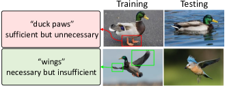
Figure 1: Example for causal sufficiency and necessity in classification problem.

Noticeably, following the causal generating mechanism, a multi-modal sample is generated simultaneously by the label and unobservable factors [22, 12], e.g., environmental effects. Existing methods [35, 65] only consider the consistency between different modalities, and will learn all generating factors, i.e., both labels and unobservable factors. Since unobservable factors are uncontrollable [46], the MML model may learn information that is different from the label semantics, resulting in the learned representations being insufficient or unnecessary. Figure 1 provides an example, given samples where all ducks with “duck paws” to classify ducks, the representation learned based on consistency will contain “duck paws”, but the model is likely to make mistakes on samples with ducks but without “duck paws” feature. It shows that the representation contains sufficient but unnecessary information, since using “duck paws” the label “duck” can be predicted, but a duck sample may not contain “duck paw”. Specifically, sufficiency indicates that use the representations will establish the label, while necessity indicates that the label becomes incorrect when the representations are absent [46]. If the MML model only focuses on causal sufficiency, it will lose important modality-specific semantics, affecting generalization; if the model only focuses on causal necessity, the decisions will be made incorrectly based on the background, affecting discriminability. Thus, existing MML methods [13, 40] without causal constraints may still fail to satisfy sufficiency and necessity, affecting model performance. The experiments in Section 6.2 further prove this (Figure 3 and Table 1): (i) the representations learned by existing methods have much lower correlation scores with sufficient and necessary causes than specifically constrains causal sufficiency and necessity; (ii) after constraining the causality of the learned representations, the performance of existing MML methods are significantly improved. We further provide a detailed example in Section 2 and Appendix B. The analyses in Section 4 also emphasize the importance of causal sufficiency and necessity. Thus, good representations for MML must with both causal sufficiency and necessity, i.e., being the causal complete causes.

In this paper, we aim to learn representations with both causal sufficiency and necessity for MML. Firstly, we propose the definition of causal complete causes ($C^{3}$) for MML, which reflects the probability of being causal necessity and sufficiency. Then, we analyze the identifiability of $C^{3}$, which allows us to quantify $C^{3}$ just using the observable data under exogeneity and monotonicity. Based on this, we propose the measurement of $C^{3}$, i.e., $C^{3}$ risk where a low $C^{3}$ risk means that the learned representations are causally necessary and sufficient with high confidence. Through theoretical analyses, we prove that $C^{3}$ risk connects the model risks on training and test data and establish a tight generalization bound for the performance guarantee. Based on these theoretical results, we propose Causal Complete Cause Regularization ($C^{3}$R), which is a plug-and-play method to learn causal complete representations by constraining their $C^{3}$ risks via the error bound.

The main contributions are as follows: (i) We define the novel causal complete cause ($C^{3}$) concept for MML, and propose the identifiability and measurement of $C^{3}$ with the constraints of exogeneity and monotonicity, i.e., $C^{3}$ risk to estimate the sufficiency and necessity of information contained in the learned representation (Section 3). (ii) Next, we theoretically demonstrate the effectiveness of $C^{3}$ risk on MML, limiting the gap between $C^{3}$ risk on the test data and the risk on the training data (Section 4). (iii) Inspired by this, we propose $C^{3}$R, which can be applied to any MML model to learn causal complete representations with low $C^{3}$ risk (Section 5). (iv) Finally, we conduct extensive experiments on various datasets that prove the effectiveness and robustness of $C^{3}$R (Section 6).

2 Problem Formulation

Problem Settings

Given a training dataset $\mathcal{D}_{tr}$ and a test dataset $\mathcal{D}_{te}$ all sampled from the multi-modal distribution $P_{XY}$, which represents the joint distribution of the samples $\mathcal{X}$ and the labels $\mathcal{Y}$. The training dataset $\mathcal{D}_{tr}$ consists of $N$ training samples, e.g., $\mathcal{D}_{tr}=\{(x^{i}_{j},y^{i}_{j})\}^{N}_{j=1}$, where each sample $x^{i}_{j}=\{x^{i}_{j,k}\}_{k=1}^{K}$ is comprised of $K$ different modalities and $y^{i}_{j}$ denotes the corresponding label. The test dataset $\mathcal{D}_{te}$ is inaccessible during training. The objective of MML is to acquire a robust and adaptable predictive function (the MML model) $f_{\theta}:\mathcal{X}\to\mathcal{Y}$ with parameters $\theta$ from $N$ training samples and $K$ data modalities to minimize prediction error on unseen test dataset $\mathcal{D}_{te}$. The expected risk of the MML model $f_{\theta}$ on the unseen test samples can be expressed as $\mathbb{E}_{(x,y)\in\mathcal{D}_{te}}[\ell(f_{\theta}(x),y)]$, where $\mathbb{E}$ is the expectation and $\ell(\cdot,\cdot)$ is the loss function.

Example of Causal Sufficiency and Necessity

As shown in Figure 1, assume that the training data is with three modalities of image, text, and audio, and all the modalities have the feature “duck paws” when a “duck” exists. The goal of this MML task is to classify the “duck”. Then, the models that learn representations based on consistency will capture the features of “duck paws”, and can establish the label “duck” based on the learned representations. However, the learned model may also make errors in another “duck” scenario where the MML samples do not contain “duck paws”, e.g., “duck swim on the lake” (upper right in Figure 1). This suggests that the learned representation contains sufficient but unnecessary causes since the label “duck” can be predicted using the current representation, but may not work in another scenario. Similarly, there are some necessary but insufficient representations, e.g., “duck” must with “wings”, but “wings” may also correspond to another label, e.g., “bird” (lower of Figure 1). For sufficient and necessary causes, they ensure that the learned representations not only reflect the features target the “duck” label, e.g., “duck paws”, but also the features where the “duck” label must have, e.g., “wings”. More examples and analyses are also described in Appendix B. Thus, good representations must have both causal sufficiency and necessity, i.e., causal complete causes, which is the goal we explore in this study.

3 Causal Complete Cause

To access the learning of causal sufficient and necessary representations, in this section, we first provide the definition of causal sufficiency and necessity in MML, i.e., Causal Complete Cause ($C^{3}$), and refine the learned modality-shared semantic representation into three parts, i.e., sufficient but unnecessary, necessary but insufficient, and sufficient and necessary causes. Next, we discuss the identifiability of $C^{3}$, which ensures the quantification of $C^{3}$ through observable data. Finally, we give the measurement of $C^{3}$, i.e., $C^{3}$ risk to measure the probability of whether one is causally complete.

3.1 Definition of Causal Complete Cause

To learn representations of modality-shared semantics $\text{F}_{c}$ that is with both causal sufficiency and necessity, based on [46], we propose the concept of Causal Complete Cause ($C^{3}$) for MML.

Definition 3.1 (Probability of Causal Complete Cause ($C^{3}$))

Assume that the data and corresponding label variables of the given multi-modal data distribution are X and Y, while the representation variable of modality-shared and modality-specific semantics are $\text{F}_{c}$ and $\text{F}_{s}$. Let the specific implementations of causal variable $\text{F}_{c}$ as $c$ and $\bar{c}$, where $\bar{c}\not=c$, and the implementations of label variable Y is $y$. The probability that $\text{F}_{c}$ is the causal complete cause of Y is:

$$\begin{split}C^{3}(\text{F}_{c}):=&\underbrace{P(\text{Y}_{do(\text{F}_{c}=c)}=y\mid\text{F}_{c}=\bar{c},\text{Y}\not=y)}_{\text{Sufficiency}}P(\text{F}_{c}=\bar{c},\text{Y}\not=y)\\ &+\underbrace{P(\text{Y}_{do(\text{F}_{c}=\bar{c})}\not=y\mid\text{F}_{c}=c,\text{Y}=y)}_{\text{Necessity}}P(\text{F}_{c}=c,\text{Y}=y),\end{split}$$ (1)

where $P(\text{Y}_{do(\text{F}_{c}=c)}=y\mid\text{F}_{c}=\bar{c},\text{Y}\not=y)$ denotes the probability of $\text{Y}=y$ when force the manipulable variable $\text{F}_{c}$ to be a fixed value with do-operator $do(\text{F}_{c}=c)$ given a certain factual observable $\text{F}_{c}=\bar{c}$ and $\text{Y}\not=y$, and the second term denotes the probability of $\text{Y}\not=y$.

The first and second terms in Definition 3.1 correspond to the probabilities of sufficiency and necessity in MML respectively. This definition indicates that when $\text{F}_{c}$ with a high $C^{3}$ score, it means that it has a high probability of being a necessary and sufficient cause of label Y. According to this definition, the representations of modality-shared semantics can be further divided into three parts: (i) Sufficient but unnecessary causes: $\text{F}_{c}$ results in effect Y, yet the presence of Y does not definitively imply that $\text{F}_{c}$ is the cause; (ii) Necessary but insufficient: the occurrence of effect Y confirms that the cause is $\text{F}_{c}$, but $\text{F}_{c}$ alone is not guaranteed to produce Y; and (iii) Sufficient and necessary causes: the presence of effect Y invariably indicates cause $\text{F}_{c}$, and conversely, the presence of $\text{F}_{c}$ invariably results in Y. We provide more examples and detailed analyses of these three parts in Appendix B.

3.2 Identifiability of Causal Complete Cause

Since it is difficult to obtain all samples in the multi-modal data distribution, especially in real systems, e.g., the counterfactual data in the definition of $C^{3}$ is difficult to obtain [36, 44], calculating the probability of $C^{3}$ is still is a challenging issue. To access the calculation of $C^{3}$ based on observable data, we discuss the identifiability of $C^{3}$ in this section. Specifically, we first provide the underlying assumptions for estimating $C^{3}$ on the counterfactual distribution of multi-modal data, i.e., exogeneity and monotonicity for $C^{3}$ (Definitions 3.2 and 3.3). Next, we propose the identifiability of $C^{3}$ under exogeneity and monotonicity (Theorem 3.4), which allows us to quantify $C^{3}$ with observable data.

We propose the definitions of exogeneity and monotonicity for $C^{3}$ based on [46] as follows:

Definition 3.2 (Exogeneity)

Variable $\text{F}_{c}$ is exogenous relative to variable Y if and only if the Y would potentially respond to conditions $c$ or $\bar{c}$ is independent of the actual value of $\text{F}_{c}$. The intervention probability is identified by conditional probability $P(\text{Y}_{do(\text{F}_{c}=c)}=y)=P(\text{Y}=y|\text{F}_{c}=c)$.

Definition 3.3 (Monotonicity)

Variable $Y$ is monotonic relative to $\text{F}_{c}$ if and only if $\text{Y}_{do(\text{F}_{c}=c)}=\bar{y}\wedge\text{Y}_{do(\text{F}_{c}=c)}=y$ is false or $\text{Y}_{do(\text{F}_{c}=\bar{c})}=y\wedge\text{Y}_{do(\text{F}_{c}=c)}=\bar{y}$ is false, where $\bar{y}\not=y$. For probabilistic formulations, $P(Y_{do(\text{F}_{c}=c)}=y,Y_{do(\text{F}_{c}=\bar{c})}\not=y)=0$ or $P(Y_{do(\text{F}_{c}=c)}\not=y,Y_{do(\text{F}_{c}=\bar{c})}=y)=0$.

Exogeneity refers to the scenario where the influence of the external intervention on the conditional distributions is negligible when the variable $\text{F}_{c}$ is exogenous relative to Y, while monotonicity illustrates the consistent, unidirectional effect on Y of causal variable $\text{F}_{c}$. Next, we propose the identifiability of $C^{3}$ under exogeneity and monotonicity based on [46].

Theorem 3.4 (Identifiability of $C^{3}$ under Exogeneity and Monotonicity)

If variable $\text{F}_{c}$ is exogenous relative to Y, and Y is monotonic relative to causal variable $\text{F}_{c}$, then we get:

$$C^{3}(\text{F}_{c})=\underbrace{P(\text{Y}=y|\text{F}_{c}=c)}_{\text{Sufficiency}}-\underbrace{P(\text{Y}=y|\text{F}_{c}=\bar{c})}_{\text{Necessity}}.$$ (2)

Theorem 3.4 posits that under conditions of exogeneity and monotonicity, the estimation of $C^{3}$ is achievable using observable multi-modal data, enabling the quantification of $C^{3}$ in the absence of counterfactual data. The proofs and more analysis are provided in Appendix A following [46, 60, 49].

3.3 Measurement of Causal Complete Cause

Based on Definition 3.1 and Theorem 3.4, we provide the measurement of $C^{3}$ in this section, i.e., $C^{3}$ risk, to estimate the $C^{3}$ score of the representation distribution $P_{\mathcal{D}_{te}}(\text{F}_{c}|\text{X}=x)$ inferred from X on the unseen test dataset $\mathcal{D}_{te}$. When the learned representation obtains less necessary and sufficient information, the $C^{3}$ risk will be higher. Specifically, we first model the predictor with representations of causal variable $\text{F}_{c}$ for decision-making (Eq.3). Then, we provide the $C^{3}$ measurement (Eq.4) of the learned $\text{F}_{c}$, i.e., $C^{3}$ risk, based on Definition 3.1. Finally, we modify the $C^{3}$ risk (Proposition 3.10) based on Theorem 3.4 to ensure compliance with the conditions of exogeneity (Theorems 3.6-3.8) and monotonicity (Theorem 3.9), accessing the calculation in practice.

Firstly, we establish the invariant predictor using a linear classifier $\mathcal{W}:\mathbb{R}^{d}\rightarrow\mathcal{Y}$ on causal representations to obtain the label $y={\rm sign}(\mathcal{W}^{\top}c)$. As the causal variable $\text{F}_{c}$ is unobservable, we infer $\text{F}_{c}$ from observable multi-modal data $x\sim\mathcal{X}$. The expected invariant predictor can be defined as:

$$\begin{split}y=\sigma[\mathbb{E}_{c\sim P_{\mathcal{D}_{te}}(\text{F}_{c}|\text{X}=x)}\mathcal{W}^{\top}{c}].\end{split}$$ (3)

where $c$ and $x$ denotes the realization of the causal variable $\text{F}_{c}$ and the data variable X, respectively, $\sigma$ denotes the signum function, and $P_{\mathcal{D}_{te}}$ is the data distribution of the MML test dataset $\mathcal{D}_{te}$.

Next, we define $C^{3}$ risk for the representation of $\text{F}_{c}$ based on Definition 3.1. Considering that the intervention value $\bar{c}$ does not necessarily come from the same distribution as $\text{F}_{c}$ [46], we define the intervention variable $\bar{\text{F}}_{c}$ has the same range as $\text{F}_{c}$, where $\bar{c}$ comes from its distribution $P_{\mathcal{D}_{te}}(\bar{\text{F}}_{c}|\text{X}=x)$ of test dataset $\mathcal{D}_{te}$. Correspondingly, the estimated distribution is defined as $P^{\theta}_{\mathcal{D}_{te}}(\text{F}_{c}|\text{X}=x)$ and $P^{\phi}_{\mathcal{D}_{te}}(\bar{\text{F}}_{c}|\text{X}=x)$, where $\theta$ and $\phi$ represent the parameters. Then, the $C^{3}$ risk is formally defined as:

$$\scalebox{0.9}{${R}_{\mathcal{D}_{te}}^{C^{3}}(\mathcal{W},\theta,\phi):=\mathbb{E}_{(x,y)\sim\mathcal{D}_{te}}\big{[}\underbrace{{\mathbb{E}}_{c\sim P_{\mathcal{D}_{te}}(\text{F}_{c}|\text{X}=x)}\rho[\sigma(\mathcal{W}^{\top}c)\neq y]}_{\text{Sufficiency}}+\underbrace{{\mathbb{E}}_{\bar{c}\sim P_{\mathcal{D}_{te}}(\bar{\text{F}}_{c}|\text{X}=x)}\rho[\sigma(\mathcal{W}^{\top}\bar{c})=y]}_{\text{Necessity}}\big{]}$},$$ (4)

where $\mathcal{W}$ is the above invariant predictor, $\rho(\cdot)$ denotes an indicator function which is equal to 1 if the condition in $\rho(\cdot)$ is true, otherwise equals 0.

To ensure the calculation of $C^{3}$ risk in practice, we modify Eq.4 based on Theorem 3.4, discussing the satisfaction of exogeneity and monotonicity. Firstly, for exogeneity, we provide a solution for finding causal representations with low $C^{3}$ risk under the following assumptions:

Assumption 3.5 (Exogeneity of $\text{F}_{c}$ in $C^{3}$ Risk)

The exogeneity of $\text{F}_{c}$ holds, if and only if the following conditions are satisfied separately: (i) $\text{X}\perp\text{Y}|\text{F}_{c}$; (ii) $\text{F}_{c}\perp\text{F}_{s}$; and (iii) ${\text{F}_{s}}\perp\text{Y}|\text{F}_{c}$.

Assumption 3.5 is consistent with a common view of MML [63, 1] that the causal variable $\text{F}_{c}\in\mathbb{R}^{d}$ maintains the invariant property across modalities (contains the primary events), i.e., $P_{A}(\text{Y}|\text{F}_{c}=c)=P_{B}(\text{Y}|\text{F}_{c}=c)$ where $A$ and $B$ denotes different modalities. Then, we define the sufficiency and necessity risks in ${R}_{\mathcal{D}_{\cdot}}^{C^{3}}(\mathcal{W},\theta,\phi)$ are denoted as ${R}_{\mathcal{D}_{\cdot}}^{suf}(\mathcal{W},\theta)$ and ${R}_{\mathcal{D}_{\cdot}}^{nec}(\mathcal{W},\phi)$, where $\mathcal{D}_{\cdot}$ denotes either the training dataset $\mathcal{D}_{tr}$ or test dataset $\mathcal{D}_{te}$. Next, we use different objectives to identify $\text{F}_{c}$ for the three causal situations with observable training data, obtaining the following theorems:

Theorem 3.6 (Objective for $\text{F}_{c}$ when $\text{X}\perp\text{Y}|\text{F}_{c}$)

The optimal learned representation of $\text{F}_{c}$ is derived from the maximization of the subsequent objective function which satisfies $\text{X}\perp\text{Y}|\text{F}_{c}$:

$$\min_{\mathcal{W},\theta}{R}_{\mathcal{D}_{tr}}^{suf}(\mathcal{W},\theta)+\lambda\mathbb{E}_{\mathcal{D}_{tr}}\mu(P_{\mathcal{D}_{tr}}^{\theta}(\text{F}_{c}|\text{X}=x)\|\pi_{\text{F}_{c}}),$$ (5)

where $\mu$ denotes the KL divergence, $\pi_{\text{F}_{c}}$ is the prior distribution which makes $\mathbb{E}_{\mathcal{D}_{tr}}\mu(P_{\mathcal{D}_{tr}}^{\theta}(\text{F}_{c}|\text{X}=x)\|\pi_{\text{F}_{c}})$ lower than a positive constant $F_{c}$ with parameter $\theta$ on the training dataset $\mathcal{D}_{tr}$.

Theorem 3.7 (Objective for $\text{F}_{c}$ when $\text{F}_{c}\perp\text{F}_{s}$)

The learned $\text{F}_{c}$ satisfies the conditional independence $\text{F}_{c}\perp\text{F}_{s}$ by optimizing the following objective with maximum mean discrepancy penalty:

$$\min_{\mathcal{W},\theta}\sum_{{s}_{i}}\sum_{{s}_{j}}\mathbb{E}_{x_{i}\sim P(\text{X}|\text{F}_{s}=s_{i})}\mathbb{E}_{c_{i}\sim P_{\mathcal{D}_{tr}}^{\theta}(\text{F}_{c}|X=x_{i})}\mathbb{E}_{x_{j}\sim P(\text{X}|\text{F}_{s}=s_{j})}\mathbb{E}_{c_{j}\sim P_{\mathcal{D}_{tr}}^{\theta}(\text{F}_{c}|X=x_{j})}\left\|c_{i}-c_{j}\right\|_{2}.$$ (6)

Theorem 3.8 (Objective for $\text{F}_{c}$ when ${\text{F}_{s}}\perp\text{Y}|\text{F}_{c}$)

The learned $\text{F}_{c}$ satisfies the conditional independence ${\text{F}_{s}}\perp\text{Y}|\text{F}_{c}$ by optimizing the following objective:

$$\min_{\mathcal{W},\theta}\sum_{s}E_{(x,y)\sim P_{\mathcal{D}_{tr}}(X,Y|\text{F}_{s}={s})}\left\|\nabla_{\mathcal{W}\mid\mathcal{W}=1.0}\mathbb{E}_{c\sim P_{\mathcal{D}_{tr}}^{\theta}(\text{F}_{c}|\text{X}=x)}\rho[\sigma(\mathcal{W}^{\top}c)\neq y]\right\|^{2}.$$ (7)

Specifically, Theorem 3.6 aims to identify invariant representation which satisfies $\text{X}\perp\text{Y}|\text{F}_{c}$, i.e., the smaller the $\mu$ value, the lower the mutual information between X and Y, which follows [50]. Theorem 3.7 satisfies $\text{F}_{c}\perp\text{F}_{s}$ by minimizing the difference of two conditional distributions $P_{\mathcal{D}_{tr}}^{\theta}(\text{F}_{c}|\text{X}=x_{i})$ and $P_{\mathcal{D}_{tr}}^{\theta}(\text{F}_{c}|\text{X}=x_{j})$ under $P(\text{X}|\text{F}_{s}=s_{i})$ and $P(\text{X}|\text{F}_{s}=s_{j})$, so that for different $\text{F}_{s}$, the expected representation of $\text{F}_{c}$ is almost the same. In other words, $\text{F}_{c}$ has nothing to do with the state of $\text{F}_{s}$, thereby achieving decoupling of semantic representations and reaching $\text{F}_{c}\perp\text{F}_{s}$. Theorem 3.8 follows IRM [4] to minimize the $L_{2}$ norm under different data conditions for a specific gradient, making the model’s prediction of $Y$ based on the learned $\text{F}_{c}$ remains unchanged under different $\text{F}_{s}$, thus satisfying ${\text{F}_{s}}\perp\text{Y}|\text{F}_{c}$. Note that the gradient calculation term in Eq.7 is consistent with the sufficient risk ${R}_{\cdot}^{suf}(\mathcal{W},\theta)$ on training dataset $\mathcal{D}_{tr}$. The proofs and more analyses are provided in Appendix A.

Next, for monotonicity, we provide a measurement $R_{\mathcal{D}_{te}}^{mon}$ to constrain monotonicity:

Theorem 3.9 (Constraint of Monotonicity)

The label $Y$ is monotonic relative to the invariant representation of $\text{F}_{c}$ if the following measurement with the highest score:

$$R_{\mathcal{D}_{te}}^{mon}(\mathcal{W},\theta,\phi):=\mathbb{E}_{(x,y)\sim\mathcal{D}_{te}}{\mathbb{E}}_{c\sim P_{\mathcal{D}_{te}}^{\theta}(\text{F}_{c}|\text{X}=x)}{\mathbb{E}}_{\bar{c}\sim P_{\mathcal{D}_{te}}^{\phi}(\bar{F}_{c}|\text{X}=x)}\rho[\sigma(\mathcal{W}^{\top}c)=\sigma(\mathcal{W}^{\top}\bar{c})].$$ (8)

Briefly, Theorem 3.9 constrain monotonicity by minimizing the difference between $c$ and $\bar{c}$ after $\sigma$ mapping under $\mathcal{W}$, ensuring that when $c$ is greater than $\bar{c}$ in ranking, the prediction $\sigma(\mathcal{W}^{\top}c)$ is also greater than $\sigma(\mathcal{W}^{\top}\bar{c})$. Then, we integrate the above constraints into $C^{3}$ risk via an upper bound.

Proposition 3.10

Consider that the sufficiency and necessity risks on test dataset $\mathcal{D}_{te}$ are ${R}_{\mathcal{D}_{te}}^{suf}(\mathcal{W},\theta)$ and ${R}_{\mathcal{D}_{te}}^{nec}(\mathcal{W},\phi)$, the labels Y and the learned causal representation of $\text{F}_{c}$ satisfies the above constraints of exogeneity and monotonicity, we get:

$$\begin{split}{R}_{\mathcal{D}_{te}}^{C^{3}}(\mathcal{W},\theta,\phi)={R}_{\mathcal{D}_{te}}^{suf}(\mathcal{W},\theta)+{R}_{\mathcal{D}_{te}}^{nec}(\mathcal{W},\phi)\leq 2{R}_{\mathcal{D}_{te}}^{suf}(\mathcal{W},\theta)+R_{\mathcal{D}_{te}}^{mon}(\mathcal{W},\theta,\phi).\end{split}$$ (9)

This upper bound explicitly takes into account monotonicity and the evaluator of sufficiency ${R}_{\mathcal{D}_{te}}^{suf}(\mathcal{W},\theta)$, while the necessity risk ${R}_{\mathcal{D}_{te}}^{nec}(\mathcal{W},\phi)$ is implicitly included in the monotonicity constraint $R_{\mathcal{D}_{te}}^{mon}(\mathcal{W},\theta,\phi)$. Note that it takes exogeneity into account as an assumption, where the constraints of exogeneity (Theorems 3.6-3.8) guide us in obtaining causally complete representations using $C^{3}$ in practice rather than being used for the modification of $C^{3}$, which will be further discussed in Section 5. The proofs of the above theorems and proposition are provided in Appendix A.

4 Theoretical Analysis for Causal Complete Cause Risk

Since the optimization of MML models only relies on the observable training data while the samples on the test set are unavailable, we cannot directly evaluate the effect of the learned multi-modal causal representations, i.e., their $C^{3}$ risks on $\mathcal{D}_{te}$. In this section, we conduct theoretical analyses to establish the connection between $C^{3}$ risk and MML performance, proving its effectiveness. Specifically, we first discuss the model risks on training and test data, i.e., the gap between ${R}_{\mathcal{D}_{tr}}^{C^{3}}(\mathcal{W},\theta,\phi)$ and ${R}_{\mathcal{D}_{te}}^{C^{3}}(\mathcal{W},\theta,\phi)$ (Theorem 4.1). Next, we provide the MML performance guarantee with a tight generalization bound via $C^{3}$ risk, i.e., using ${R}_{\mathcal{D}_{tr}}^{suf}(\mathcal{W},\theta)$ and ${R}_{\mathcal{D}_{tr}}^{nec}(\mathcal{W},\phi)$ of ${R}_{\mathcal{D}_{tr}}^{C^{3}}(\mathcal{W},\theta,\phi)$ to describe the gap boundary between expected and empirical errors (Theorem 4.2).

Theorem 4.1 (Training and Test Risks Connection via $C^{3}$)

Let the distance between the training dataset $\mathcal{D}_{tr}$ and test dataset $\mathcal{D}_{te}$ as $L_{d}^{t}=[\mathbb{E}_{(x,y)\sim\mathcal{D}_{tr}}(\frac{\mathcal{D}_{tr}(x,y)}{\mathcal{D}_{te}(x,y)})^{t}]^{\frac{1}{t}}$ following [17], then the $C^{3}$ risk ${R}_{\mathcal{D}_{te}}^{C^{3}}(\mathcal{W},\theta,\phi)$ on the test dataset is bounded by the risk ${R}_{\mathcal{D}_{tr}}^{C^{3}}(\mathcal{W},\theta,\phi)$ on the training dataset:

$$\scalebox{0.9}{${R}_{\mathcal{D}_{te}}^{C^{3}}(\mathcal{W},\theta,\phi)\leq\underset{t\rightarrow+\infty}{\lim}L_{d}^{t}(2[{R}_{\mathcal{D}_{tr}}^{suf}(\mathcal{W},\theta)]^{1-\frac{1}{t}}+[{R}_{\mathcal{D}_{tr}}^{mon}(\mathcal{W},\theta,\phi)]^{1-\frac{1}{t}})+P_{\mathcal{D}_{te}\setminus\mathcal{D}_{tr}}\cdot\sup{R}_{\mathcal{D}_{te}\setminus\mathcal{D}_{tr}}^{C^{3}}(\mathcal{W},\theta,\phi)$},$$ (10)

where $P_{\mathcal{D}_{te}\setminus\mathcal{D}_{tr}}\cdot\sup{R}_{\mathcal{D}_{te}\setminus\mathcal{D}_{tr}}^{C^{3}}(\mathcal{W},\theta,\phi)$ denotes the expectation of worst risk on unknown MML data when not obtain the modality-shared information on the observable training data following [74, 48, 4]. When the learned causal representation of $\text{F}_{c}$ is the invariant representation in ideal cases, i.e., $P_{\mathcal{D}_{tr}}(\text{Y}|\text{F}_{c}=c)=P_{\mathcal{D}_{te}}(\text{Y}|\text{F}_{c}=c)$, the $P_{\mathcal{D}_{te}\setminus\mathcal{D}_{tr}}\cdot\sup{R}_{\mathcal{D}_{te}\setminus\mathcal{D}_{tr}}^{C^{3}}(\mathcal{W},\theta,\phi)$ approaches to 0 and the bound will be:

$${R}_{\mathcal{D}_{te}}^{C^{3}}(\mathcal{W},\theta,\phi)\leq\underset{t\rightarrow+\infty}{\lim}L_{d}^{t}(2[{R}_{\mathcal{D}_{tr}}^{suf}(\mathcal{W},\theta)]^{1-\frac{1}{t}}+[{R}_{\mathcal{D}_{tr}}^{mon}(\mathcal{W},\theta,\phi)]^{1-\frac{1}{t}}).$$ (11)

Theorem 4.1 provides a link between the risk of the MML model on the training and the test datasets. Note that although it is difficult for us to access all the data of the test dataset during training, since $P_{\mathcal{D}_{te}}$ and $P_{\mathcal{D}_{tr}}$ come from the same multimodal data distribution $P_{XY}$, we can directly estimate $L_{d}^{t}$ and ${R}_{\mathcal{D}_{tr}}^{mon}(\mathcal{W},\theta,\phi)$ [74, 65]. This value can be considered as a priori hyperparameter in practice.

Next, we provide the relationship between $C^{3}$ risk and MML generalization. MML generalization describes the difference between the empirical risk of MML models on observable training data and the expected risk on unobservable test data distribution [64, 67]. The theorem of MML generalization guarantee via $C^{3}$, i.e., the upper bound of the risk gap, is formulated as follows:

Theorem 4.2 (Performance Guarantee via $C^{3}$)

Given the multi-modal training dataset $\mathcal{D}_{tr}$ with $N$ observable samples, the parameters $\theta$ and $\phi$, let $\pi_{\text{F}_{c}}$ and $\pi_{\bar{\text{F}}_{c}}$ are the prior distributions that make $\mathbb{E}_{\mathcal{D}_{tr}}\mu(P_{\mathcal{D}_{tr}}^{\theta}(\text{F}_{c}|\text{X}=x)\|\pi_{\text{F}_{c}})$ and $\mathbb{E}_{\mathcal{D}_{tr}}\mu(P_{\mathcal{D}_{tr}}^{\phi}(\bar{\text{F}}_{c}|\text{X}=x)\|\pi_{\bar{\text{F}}_{c}})$ lower than the positive constants $F_{c}$ for any $\mathcal{W}:\mathbb{R}^{d}\rightarrow\mathcal{Y}$, then we get the bounds for the risk gaps of ${R}_{\mathcal{D}_{\cdot}}^{suf}(\mathcal{W},\theta)$ and ${R}_{\mathcal{D}_{\cdot}}^{mon}(\mathcal{W},\theta,\phi)$ (two terms of Eq.9 and Eq.11) with a probability at least $1-\varepsilon$ where $0<\varepsilon<1$, respectively. For the sufficiency term ${R}_{\mathcal{D}_{\cdot}}^{suf}(\mathcal{W},\theta)$, we get:

$$\scalebox{0.9}{$|{R}_{\mathcal{D}_{te}}^{suf}(\mathcal{W},\theta)-{R}_{\mathcal{D}_{tr}}^{suf}(\mathcal{W},\theta)|\leq\mathbb{E}_{\mathcal{D}_{tr}}\mu(P_{\mathcal{D}_{tr}}^{\theta}(\text{F}_{c}|\text{X}=x)\|\pi_{\text{F}_{c}})+\frac{\ln(N/\varepsilon)}{N}+\mathcal{O}(1)$}.$$ (12)

Next, for the monotonicity term ${R}_{\mathcal{D}_{\cdot}}^{mon}(\mathcal{W},\theta,\phi)$, we get:

$$\scalebox{0.82}{$|{R}_{\mathcal{D}_{te}}^{mon}(\mathcal{W},\theta,\phi)-{R}_{\mathcal{D}_{tr}}^{mon}(\mathcal{W},\theta,\phi)|\leq\mathbb{E}_{\mathcal{D}_{tr}}\mu(P_{\mathcal{D}_{tr}}^{\theta}(\text{F}_{c}|\text{X}=x)\|\pi_{\text{F}_{c}})+\mathbb{E}_{\mathcal{D}_{tr}}\mu(P_{\mathcal{D}_{tr}}^{\phi}(\bar{\text{F}}_{c}|\text{X}=x)\|\pi_{\bar{\text{F}}_{c}})+\frac{\ln(N/\varepsilon)}{N}+\mathcal{O}(1)$}.$$ (13)

Theorem 4.2 provides a connection between $C^{3}$ and MML generalization, while obtaining that as the KL divergence term decreases and the observable sample size increases, the generalization of MML models will become better. Meanwhile, combined with the above Theorems 4.1 and 4.2, we can evaluate the effect of the learned representations via $C^{3}$ on the training data, i.e., the expected $C^{3}$ risk on the unseen test distribution. This inspired us to propose a $C^{3}$-based method to learn causal complete representations, which is illustrated in Section 5. The proofs are provided in Appendix A.

5 Learning Causal Complete Representations

In this section, we propose a plug-and-play method, namely Causal Complete Cause Regularization ($C^{3}$R), which is built upon the $C^{3}$ risk to extract causal complete representations from observable multi-modal data for MML. Specifically, we first introduce the exogeneity and monotonicity constraints (Theorems 3.6-3.9) to make the semantics separable and learn invariant representations to satisfy the causal assumptions (Assumption 3.5) in practice. Then, we minimize the $C^{3}$ risk of the learned representations, i.e., minimizing the upper bound of the $C^{3}$ risk based on Theorems 4.1 and 4.2, to ensure the causal completeness of the learned representation, i.e., causal sufficiency and necessity. In summary, the objective of $C^{3}$R is a combination of the above two-step objective functions, which can be embedded in various MML models and illustrated below.

Overall Objective

Note that reviewing the upper bound of $C^{3}$ risk, there is another issue that remains to be considered before optimizing, i.e., given the variety of choices for $P^{\phi}(\bar{\text{F}}_{c}|\text{X}=x)$, there are several possible $C^{3}$ risks. For this issue, during the multi-modal representation learning phase, we prioritize minimizing the worst-case $C^{3}$ risk dictated by $\bar{\text{F}}_{c}$, specifically the maximum risk associated with the selection of $P^{\phi}(\bar{\text{F}}_{c}|\text{X}=x)$. Then, combining the regular terms in Theorems 3.6-3.9, the optimization process of the objectives presented in Theorems 4.1 and 4.2, i.e., minimizing the $C^{3}$ risk upper bounds of the learned MML representations to achieve causal completeness, will becomes:

$$\begin{split}\scalebox{0.92}{$\underset{\theta,\mathcal{W}}{\min}\underset{\phi}{\max}{R}_{\mathcal{D}_{tr}}^{suf}(\mathcal{W},\theta)+{R}_{\mathcal{D}_{tr}}^{mon}(\mathcal{W},\theta,\phi)+\lambda_{1}\mathcal{L}_{\mu}(\mathcal{W},\theta,\phi)+\lambda_{2}\mathcal{L}_{\text{F}_{c}\perp\text{F}_{s}}(\mathcal{W},\theta)+\lambda_{3}\mathcal{L}_{\text{F}_{s}\perp\text{Y}|\text{F}_{c}}(\mathcal{W},\theta)$},\end{split}$$ (14)

where $\lambda_{1}$, $\lambda_{2}$, and $\lambda_{3}$ are the weight of three regular terms, i.e., the KL divergence term $\mathcal{L}_{\mu}:=\mathbb{E}_{\mathcal{D}_{tr}}\mu(P_{\mathcal{D}_{tr}}^{\theta}(\text{F}_{c}|\text{X}=x)\|\pi_{\text{F}_{c}})+\mathbb{E}_{\mathcal{D}_{tr}}\mu(P_{\mathcal{D}_{tr}}^{\phi}(\bar{\text{F}}_{c}|\text{X}=x)\|\pi_{\bar{\text{F}}_{c}})$, the semantic separable constraint $\mathcal{L}_{\text{F}_{c}\perp\text{F}_{s}}$ in Theorem 3.7, and the conditionally independent constraint $\mathcal{L}_{\text{F}_{s}\perp\text{Y}|\text{F}_{c}}$ (Theorem 3.8). Note that the remaining constraints on exogeneity (Theorem 3.6) and monotonicity (Theorem 3.9) have already been integrated into the upper bound of $C^{3}$ risk as originally described in Theorems 3.6-3.9, i.e., consistent with the main items of the upper bounds, which implicitly makes $\text{F}_{c}$ satisfy the property of exogeneity and monotonicity under the corresponding causal assumption. Briefly, by minimizing the upper bound of $C^{3}$ risk, the $C^{3}$ score of the learned representation will be higher, thus making the learned representation causally sufficient and necessary with high confidence.

6 Experiments

In this section, we conduct extensive experiments on various benchmark datasets to verify the effectiveness of $C^{3}$R. More details and additional experiments are provided in Appendix C-F.

Table 1: Performance comparison when 50% of the modalities are corrupted with Gaussian noise i.e., zero mean with the variance of $N$. “(N, Avg.)” and “(N, Worst.)” denotes the average and worst-case accuracy. The best results are highlighted in bold. Full results are provided in Appendix F.

Method	NYU Depth V2				SUN RGB-D				FOOD 101				MVSA
	(0,Avg.)	(0,Worst.)	(10,Avg.)	(10,Worst.)	(0,Avg.)	(0,Worst.)	(10,Avg.)	(10,Worst.)	(0,Avg.)	(0,Worst.)	(10,Avg.)	(10,Worst.)	(0,Avg.)	(0,Worst.)	(10,Avg.)	(10,Worst.)
CLIP [53]	69.32	68.29	51.67	48.54	56.24	54.73	35.65	32.76	85.24	84.20	52.12	49.31	62.48	61.22	31.64	28.27
ALIGN [24]	66.43	64.33	45.24	42.42	57.32	56.26	38.43	35.13	86.14	85.00	53.21	50.85	63.25	62.69	30.55	26.44
MaPLe [31]	71.26	69.27	52.98	48.73	62.44	61.76	34.51	30.29	90.40	86.28	53.16	40.21	77.43	75.36	43.72	38.82
CoOp [25]	67.48	66.94	49.43	45.62	58.36	56.31	39.67	35.43	88.33	85.10	55.24	51.01	74.26	73.61	42.58	37.29
VPT [25]	62.16	61.21	41.05	37.81	54.72	53.92	33.48	29.81	83.89	82.00	51.44	49.01	65.87	64.98	32.79	29.21
Late fusion [56]	69.14	68.35	51.99	44.95	62.09	60.55	47.33	44.60	90.69	90.58	58.00	55.77	76.88	74.76	55.16	47.78
ConcatMML [72]	70.30	69.42	53.20	47.71	61.90	61.19	45.64	42.95	89.43	88.79	56.02	54.33	75.42	75.33	53.42	50.47
AlignMML [56]	70.31	68.50	51.74	44.19	61.12	60.12	44.19	38.12	88.26	88.11	55.47	52.76	74.91	72.97	52.71	47.03
ConcatBow [69]	49.64	48.66	31.43	29.87	41.25	40.54	26.76	24.27	70.77	70.68	35.68	34.92	64.09	62.04	45.40	40.95
ConcatBERT [69]	70.56	69.83	44.52	43.29	59.76	58.92	45.85	41.76	88.20	87.81	49.86	47.79	65.59	64.74	46.12	41.81
MMTM [30]	71.04	70.18	52.28	46.18	61.72	60.94	46.03	44.28	89.75	89.43	57.91	54.98	74.24	73.55	54.63	49.72
TMC [20]	71.06	69.57	53.36	49.23	60.68	60.31	45.66	41.60	89.86	89.80	61.37	61.10	74.88	71.10	60.36	53.37
LCKD [55]	68.01	66.15	42.31	40.56	56.43	56.32	43.21	42.43	85.32	84.26	47.43	44.22	62.44	62.27	43.52	38.63
UniCODE [63]	70.12	68.74	44.78	42.79	59.21	58.55	46.32	42.21	88.39	87.21	51.28	47.95	66.97	65.94	48.34	42.95
SimMMDG [13]	71.34	70.29	45.67	44.83	60.54	60.31	47.86	45.79	89.57	88.43	52.55	50.31	67.08	66.35	49.52	44.01
MMBT [32]	67.00	65.84	49.59	47.24	56.91	56.18	43.28	39.46	91.52	91.38	56.75	56.21	78.50	78.04	55.35	52.22
QMF [69]	70.09	68.81	55.60	51.07	62.09	61.30	48.58	47.50	92.92	92.72	62.21	61.76	78.07	76.30	61.28	57.61
CLIP+$C^{3}$R	75.98	74.28	56.32	52.23	61.39	58.17	40.86	37.24	92.25	90.74	58.91	56.39	68.94	68.15	38.62	34.73
MaPLe+$C^{3}$R	76.21	73.54	58.26	54.91	64.86	64.63	39.04	36.82	93.71	92.26	59.57	45.83	81.03	80.93	48.95	45.31
Late fusion+$C^{3}$R	72.57	71.23	56.78	49.84	64.15	62.31	52.96	49.37	93.66	92.05	64.32	58.61	83.44	79.28	61.86	52.08
LCKD+$C^{3}$R	75.83	73.84	48.95	47.31	60.11	59.65	45.99	45.13	90.01	89.23	53.84	50.77	66.41	65.06	48.45	42.00
SimMMDG+$C^{3}$R	74.39	73.98	49.15	46.22	64.34	63.50	51.54	51.01	91.55	90.12	56.38	53.15	72.77	70.42	51.36	50.88
MMBT+$C^{3}$R	72.87	70.93	53.29	51.30	60.32	59.18	47.89	45.19	93.89	93.22	60.23	59.55	82.64	81.27	61.81	58.19
QMF+$C^{3}$R	76.56	74.01	58.54	58.13	66.77	64.90	51.15	50.00	94.25	93.41	65.33	62.74	82.56	81.37	66.37	64.02

Table 2: Performance with missing modalities on BraTS. The brackets indicate the effect changes after introducing $C^{3}$R. “$\bullet$” and “$\circ$” indicate the availability and absence of the modality for testing.

Modalities				Enhancing Tumour						Tumour Core						Whole Tumour
Fl	T1	T1c	T2	HMIS	HVED	RSeg	mmFm	LCKD	LCKD+$C^{3}$R	HMIS	HVED	RSeg	mmFm	LCKD	LCKD+$C^{3}$R	HMIS	HVED	RSeg	mmFm	LCKD	LCKD+$C^{3}$R
$\bullet$	$\circ$	$\circ$	$\circ$	11.78	23.80	25.69	39.33	45.48	49.56 (+4.08)	26.06	57.90	53.57	61.21	72.01	76.31 (+4.30)	52.48	84.39	85.69	86.10	89.45	91.50 (+2.05)
$\circ$	$\bullet$	$\circ$	$\circ$	10.16	8.60	17.29	32.53	43.22	48.59 (+5.47)	37.39	33.90	47.90	56.55	66.58	72.04 (+5.46)	57.62	49.51	70.11	67.52	76.48	82.12 (+5.64)
$\circ$	$\circ$	$\bullet$	$\circ$	62.02	57.64	67.07	72.60	75.65	79.86 (+4.21)	65.29	59.59	76.83	75.41	83.02	87.67 (+4.65)	61.53	53.62	73.31	72.22	77.23	81.72 (+4.49)
$\circ$	$\circ$	$\circ$	$\bullet$	25.63	22.82	28.97	43.05	47.19	53.64 (+6.45)	57.20	54.67	57.49	64.20	70.17	76.56 (+6.39)	80.96	79.83	82.24	81.15	84.37	90.54 (+6.17)
$\bullet$	$\bullet$	$\circ$	$\circ$	10.71	27.96	32.13	42.96	48.30	53.82 (+4.52)	41.12	61.14	60.68	65.91	74.58	78.85 (+4.27)	64.62	85.71	88.24	87.06	89.97	93.02 (+3.05)
$\bullet$	$\circ$	$\bullet$	$\circ$	66.10	68.36	70.30	75.07	78.75	82.61 (+3.86)	71.49	75.07	80.62	77.88	85.67	89.10 (+3.43)	68.99	85.93	88.51	87.30	90.47	93.73 (+3.26)
$\bullet$	$\circ$	$\circ$	$\bullet$	30.22	32.31	33.84	47.52	49.01	55.74 (+6.73)	57.68	62.70	61.16	69.75	75.41	82.38 (+6.97)	82.95	87.58	88.28	87.59	90.39	94.81 (+4.42)
$\circ$	$\bullet$	$\bullet$	$\circ$	66.22	61.11	69.06	74.04	76.09	81.23 (+5.14)	72.46	67.55	78.72	78.59	82.49	88.03 (+5.54)	68.47	64.22	77.18	74.42	80.10	86.05 (+5.95)
$\circ$	$\bullet$	$\circ$	$\bullet$	32.39	24.29	32.01	44.99	50.09	55.15 (+5.06)	60.92	56.26	62.19	69.42	72.75	78.02 (+5.27)	82.41	81.56	84.78	82.20	86.05	91.39 (+5.34)
$\circ$	$\circ$	$\bullet$	$\bullet$	67.83	67.83	69.71	74.51	76.01	83.33 (+7.32)	76.64	73.92	80.20	78.61	84.85	92.50 (+7.65)	82.48	81.32	85.19	82.99	86.49	93.56 (+7.07)
$\bullet$	$\bullet$	$\bullet$	$\circ$	68.54	68.60	70.78	75.47	77.78	82.35 (+4.57)	76.01	77.05	81.06	79.80	85.24	89.52 (+4.28)	72.31	86.72	88.73	87.33	90.50	94.89 (+4.39)
$\bullet$	$\bullet$	$\circ$	$\bullet$	31.07	32.34	36.41	47.70	49.96	55.87 (+5.91)	60.32	63.14	64.38	71.52	76.68	82.00 (+5.32)	83.43	88.07	88.81	87.75	90.46	95.70 (+5.24)
$\bullet$	$\circ$	$\bullet$	$\bullet$	68.72	68.93	70.88	75.67	77.48	83.52 (+6.04)	77.53	76.75	80.72	79.55	85.56	92.20 (+6.64)	83.85	88.09	89.27	88.14	90.90	95.83 (+4.93)
$\circ$	$\bullet$	$\bullet$	$\bullet$	69.92	67.75	70.10	74.75	77.60	82.18 (+4.58)	78.96	75.28	80.33	80.39	84.02	88.76 (+4.74)	83.94	82.32	86.01	82.71	86.73	91.19 (+4.46)
$\bullet$	$\bullet$	$\bullet$	$\bullet$	70.24	69.03	71.13	77.61	79.33	85.45 (+6.12)	79.48	77.71	80.86	85.78	85.31	90.86 (+5.55)	84.74	88.46	89.45	89.64	90.84	95.02 (+4.18)

Figure 2: Evaluation for the property of learned representations (identification for SNC, SC, NC, and SP). See Appendix F for more results.

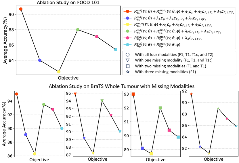
Figure 3: Ablation study for $C^{3}$R, i.e., performance when removing (“$-$”) the corresponding regular terms. See Appendix F for more results.

6.1 Experimental Settings

Datasets

We select four MML tasks with six datasets: (i) scenes recognition on NYU Depth V2 [51] and SUN RGBD [52] with RGB and depth images; (ii) image-text classification on UPMC FOOD101 [59] and MVSA [45] with image and text; (iii) segmentation considering missing modalities on BraTS [43, 5] with Flair, T1, T1c, and T2; and (iv) synthetic MMLSynData (see Appendix B.1).

Implementation Details

We use a three-layer MLP with activation functions [10] as the representation learner. The hidden vector dimensions of each layer are specified as 64, 32, and 128, while the learned representation is 64. We embed this network into MML models to predict labels. For optimization, we employ the Adam optimizer [33] with Momentum and weight decay set at $0.8$ and $10^{-4}$. The initial learning rate is established at 0.1, with the flexibility for linear scaling as required. Additionally, we use grid search to set the hyperparameters $\lambda_{1}=0.01$, $\lambda_{2}=0.55$, and $\lambda_{3}=0.4$. All experimental procedures are executed using NVIDIA RTX A6000 GPUs.

6.2 Results

Performance and robustness analysis

To evaluate the effectiveness and robustness of $C^{3}$R, we record the average and worst-case accuracy of various MML baselines and introduce $C^{3}$R under Gaussian noise (for image modality) and blank noise (for text modality) following [20, 70, 41]. The results are shown in Table 1. We can observe that $C^{3}$R achieves stable improvements in both the average and worst-case accuracy. This proves the superior effectiveness and robustness of $C^{3}$R.

When faces the problem of missing modalities

Considering the missing modalities problem faced by MML in reality, we evaluate the performance of $C^{3}$R and several strong baselines [55, 5, 71] on all 15 possible combinations of missing modalities on BraTS. From the results shown in Table 2, we can observe that (i) $C^{3}$R brings significant performance improvements; (ii) $C^{3}$R can reduce the learning gap for the representations on different modal semantics, i.e., reducing the accuracy gap of learning on the difficult-to-identify Fl and T1 modalities and the easy T1c. This demonstrates the superiority of $C^{3}$R and the advantage of causally complete representation in missing modality issues.

Learning causal complete representations

To evaluate $C^{3}$R’s ability to extract causal complete causes, we conduct experiments with two steps: (i) construct four types of MML data, i.e., sufficient and necessary (SNC), sufficient but unnecessary (SC), necessary but insufficient causes (NC), and spurious correlations (SP) following [65] (see Appendix F for more details); then (ii) evaluate their correlation with the learned representation of $\text{F}_{c}$ based on the distance metric [28], i.e., the higher the score, the stronger the correlation. The results are shown in Figure 3 (see Appendix B and F for more results). The representation learned by $C^{3}$R contains better causal sufficiency and necessity, i.e., has a higher correlation with SNC and lower with SP. This proves that $C^{3}$R can learn causal complete representations more effectively while other methods are hard to achieve this.

Ablation Study

To evaluate the effect of each item in the $C^{3}$R objective (Eq.14), we evaluate the performance change on LCKD+$C^{3}$R after eliminating the corresponding regularization term in the objective (Eq.14). We consider the standard and corner case, i.e., with missing modality, and conduct experiments on FOOD 101 and BraTS, as shown in Figure 3. We can observe that each item of the model objective plays an important role, especially the ${R}_{\mathcal{D}_{tr}}^{suf}$ and ${R}_{\mathcal{D}_{tr}}^{mon}$. Meanwhile, we also conduct experiments for model efficiency and parameter sensitivity, as illustrated in Appendix F.

7 Related Work

Multi-modal learning aims to learn unified representations through two or more modalities and then apply them to unseen samples. Recently, multiple methods [64, 26, 57, 15] have been proposed to solve MML tasks, e.g., unified models tokenize diverse input modalities into sequences and utilize Transformer for joint learning [7, 58], whereas CLIP [47, 15], ALIGN [24], etc. employ distinct encoders for each modality and utilize contrastive loss to synchronize features. These methods align features from different modalities into the same space, where the learned representations are considered to contain the primary events. However, they rely on the semantic alignment assumption [3, 57] or using a fixed single vector to learn [40, 68] while ignoring the completeness of the learned representation, e.g., only visual appearance but ignore contextual features in video data. This results in the model being limited to pure data while difficult to perform well on downstream tasks [18, 67]. Although recent works [27, 13, 54, 62] proposed to divide the MML features into different components, i.e., features for modality-specific and modality-shared semantics, and learn the latter which is invariant across modalities. However, they also ignore causal completeness, resulting in learned representations that may contain incomplete or insufficient information [46] and are prone to problems such as missing modality in real life. In this paper, we propose to constrain learning causal complete representations (causes) from a causal perspective instead of just learning modality-shared semantics to ensure that important and general information is retained.

8 Conclusion

In this paper, we explore and promote the learning of causal sufficient and necessary representations for MML. To measure whether the learned representation is causally complete, we present the definition, identifiability, and measurement of $C^{3}$ with theoretical supports. Based on these results, we propose a plug-and-play method $C^{3}$R to promote MML learn causal complete representations. Extensive experiments conducted on various benchmark datasets demonstrate its effectiveness.

Limitations This work focuses on the general MML cases and is not analyzed for unsupervised settings. We will study more cases, e.g., self-supervised MML to further extend this work.

Broader Impacts This work provides strict definitions and theorems for causal complete causes in MML, and further proposes a plug-and-play method for learning causal complete representations. Extensive theoretical and empirical analyses have proven its effectiveness and robustness. This work opens up interesting future research directions, which is another exciting topic for future works.

Appendix

This supplementary material provides results for additional experiments and details to reproduce our results that could not be included in the paper submission due to space limitations.

• Appendix A provides proofs and further theoretical analysis of the theory in the text.

• Appendix B provides discussions of how to better understand $C^{3}$ score, and the three parts of learned invariant representations, i.e., sufficient but unnecessary, necessary but insufficient, and sufficient and necessary causes.

• Appendix C provides the additional details of the benchmark datasets.

• Appendix D provides the additional details of the baselines for comparision.

• Appendix E provides the additional details of the implementation details.

• Appendix F provides the full results and additional experiments for the evaluation of $C^{3}$R. Note that before we illustrate the details and analysis, we provide a brief summary about all the experiments conducted in this paper, as shown in Table 3.

Table 3: Illustration of the experiments conducted in this work. Note that all experimental results are obtained after five rounds of experiments.

Experiments	Location	Results
Performance and robustness analysis	Section 6.2 and Appendix F.1	Table 1, Table 4, and Table 5
Performance comparison when faces the problem of missing modalities	Section 6.2 and Appendix F.2	Table 2
Performance of learning causal complete representations	Section 6.2, Appendix B.1, and Appendix F.3	Figure 3 and Figure 5
Ablation Study about the effect of each item in the $C^{3}$R objective (Eq.14)	Section 6.2 and Appendix F.4	Figure 3
Experiment of model efficiency	Appendix F.4	Figure 7
Experiment of parameter sensitivity	Appendix F.4	Figure 7, Figure 9, and Figure 9

Appendix A Proofs

In this section, we provide the proofs of (i) the $C^{3}$ identifiability (Theorem 3.4), (ii) the satisfaction of exogeneity and monotonicity (Theorems 3.6-3.9), (ii) the risk bounds when modifying the $C^{3}$ risk (Proposition 3.10), and (iv) the performance guarantee (theoretical analysis) for $C^{3}$ risk (Theorem 4.1 and Theorem 4.2).

A.1 Proof of Theorem 3.4

Theorem 3.4 (Identifiability of $C^{3}$ under Exogeneity and Monotonicity)

If variable $\text{F}_{c}$ is exogenous relative to Y, and Y is monotonic relative to causal variable $\text{F}_{c}$, then we get:

$$C^{3}(\text{F}_{c})=\underbrace{P(\text{Y}=y|\text{F}_{c}=c)}_{\text{Sufficiency}}-\underbrace{P(\text{Y}=y|\text{F}_{c}=\bar{c})}_{\text{Necessity}}.$$

Proof

Following [46], writing $\text{Y}_{\bar{c}}\vee\bar{\text{Y}}_{\bar{c}}=true$, we have:

$$\text{Y}_{c}=\text{Y}_{c}\wedge(\text{Y}_{\bar{c}}\vee\bar{\text{Y}}_{\bar{c}})=(\text{Y}_{c}\wedge\text{Y}_{\bar{c}})\vee(\text{Y}_{c}\wedge\bar{\text{Y}}_{\bar{c}}),$$ (15)

and

$$\text{Y}_{\bar{c}}=\text{Y}_{\bar{c}}\wedge(\text{Y}_{c}\vee\bar{\text{Y}}_{c})=(\text{Y}_{\bar{c}}\wedge\text{Y}_{c})\vee(\text{Y}_{\bar{c}}\wedge\bar{\text{Y}}_{c})=\text{Y}_{\bar{c}}\wedge\text{Y}_{c}.$$ (16)

Since monotonicity entails $\text{Y}_{\bar{c}}\vee\bar{\text{Y}}_{\bar{c}}=false$, Substituting Eq.16 into Eq.15 yields:

$$\text{Y}_{c}=\text{Y}_{\bar{c}}\vee(\text{Y}_{c}\wedge\bar{\text{Y}}_{\bar{c}}).$$ (17)

Taking the probability form and using the disjointness of $\text{Y}_{\bar{c}}$ and $\bar{\text{Y}}_{\bar{c}}$ on the test dataset $\mathcal{D}_{te}$ as an example, we can obtain:

$$P_{\mathcal{D}_{te}}(\text{Y}=y|\text{F}_{c}=c)=P_{\mathcal{D}_{te}}(\text{Y}=y|\text{F}_{c}=\bar{c})+P_{\mathcal{D}_{te}}(\text{Y}=y|\text{F}_{c}=c,\text{Y}=\bar{y}|\text{F}_{c}=\bar{c}),$$ (18)

where $P_{\mathcal{D}_{te}}(\text{Y}=y|\text{F}_{c}=c,\text{Y}=\bar{y}|\text{F}_{c}=\bar{c})$ corresponding to $C^{3}(\text{F}_{c})$, we get:

$$C^{3}(\text{F}_{c})=P_{\mathcal{D}_{te}}(\text{Y}=y|\text{F}_{c}=c)-P_{\mathcal{D}_{te}}(\text{Y}=y|\text{F}_{c}=\bar{c}).$$ (19)

A.2 Proofs of Theorems 3.6-3.9

In this section, we provide the proofs of exogeneity and monotonicity constraints, as mentioned in Section 3.3. Firstly, we provide the proofs of exogeneity constraints (Theorems 3.6-3.8). Before the proof, we give the assumption and theorems of the relevant constraints.

Assumption 3.5 (Exogeneity of $\text{F}_{c}$ in $C^{3}$ Risk)

The exogeneity of $\text{F}_{c}$ holds, if and only if the following conditions are satisfied separately: (i) $\text{X}\perp\text{Y}|\text{F}_{c}$; (ii) $\text{F}_{c}\perp\text{F}_{s}$; and (iii) ${\text{F}_{s}}\perp\text{Y}|\text{F}_{c}$.

Next, we provide the proofs of Theorems 3.6-3.8.

Theorem 3.6 (Objective for $\text{F}_{c}$ when $\text{X}\perp\text{Y}|\text{F}_{c}$)

The optimal learned representation of $\text{F}_{c}$ is derived from the maximization of the subsequent objective function which satisfies $\text{X}\perp\text{Y}|\text{F}_{c}$:

$$\min_{\mathcal{W},\theta}{R}_{\mathcal{D}_{tr}}^{suf}(\mathcal{W},\theta)+\lambda\mathbb{E}_{\mathcal{D}_{tr}}\mu(P_{\mathcal{D}_{tr}}^{\theta}(\text{F}_{c}|\text{X}=x)\|\pi_{\text{F}_{c}}),$$

where $\mu$ denotes the KL divergence, $\pi_{\text{F}_{c}}$ is the prior distribution which makes $\mathbb{E}_{\mathcal{D}_{tr}}\mu(P_{\mathcal{D}_{tr}}^{\theta}(\text{F}_{c}|\text{X}=x)\|\pi_{\text{F}_{c}})$ lower than a positive constant $F_{c}$ with parameter $\theta$ on the training dataset $\mathcal{D}_{tr}$.

Proof

we provide the proof and demonstrate why minimizing the objective is equivalent to finding the $\text{F}_{c}$ satisfying conditional independence, which is also the main term in the $C^{3}$ risk. Specifically, we first prove the optimization of this objective (Eq.5) is equivalent to the Information Bottleneck (IB) objective mentioned in [50], i.e., $\mathcal{L}=\max{I}(\text{F}_{c},\text{Y})-\lambda{I}(\text{X},\text{F}_{c})$, where ${I}(A,B)$ denotes the mutual information between $A$ and $B$. $\text{X},\text{Y}$ are from $\mathcal{D}_{tr}$. Next, we prove the optimal solution of Information Bottleneck satisfies $\text{X}\perp\text{Y}|\text{F}_{c}$.

Firstly, we prove that this objective is equivalent to the Information Bottleneck (IB) objective. We start by bounding ${I}(\text{F}_{c},\text{Y})$ and ${I}(\text{X},\text{F}_{c})$ separately. Regarding the term $I(\text{F}_{c},\text{Y})$, we get:

$$I(\text{F}_{c},\text{Y})=\int P_{\mathcal{D}_{tr}}(\text{Y},\text{F}_{c})\log\frac{P_{\mathcal{D}_{tr}}(\text{Y},\text{F}_{c})}{P_{\mathcal{D}_{tr}}(\text{Y})P_{\mathcal{D}_{tr}}(\text{F}_{c})}d\text{Y}d\text{F}_{c}=\int P_{\mathcal{D}_{tr}}(\text{Y},\text{F}_{c})\log\frac{P_{\mathcal{D}_{tr}}(\text{Y}\mid\text{F}_{c})}{P_{\mathcal{D}_{tr}}(\text{Y})}d\text{Y}d\text{F}_{c}.$$ (20)

for the specific term $P_{\mathcal{D}_{tr}}(\text{Y},\text{F}_{c})$:

$$\scalebox{0.9}{$P_{\mathcal{D}_{tr}}(\text{Y}\mid\text{F}_{c})=\int P_{\mathcal{D}_{tr}}(\text{X},\text{Y}\mid\text{F}_{c})d\text{X}=\int P_{\mathcal{D}_{tr}}(\text{Y}\mid\text{X})P_{\mathcal{D}_{tr}}(\text{X}\mid\text{F}_{c})d\text{X}=\int\frac{P_{\mathcal{D}_{tr}}(\text{Y}\mid\text{X})P^{\theta}_{\mathcal{D}_{tr}}(\text{F}_{c}\mid\text{X})P_{\mathcal{D}_{tr}}(\text{X})}{P_{\mathcal{D}_{tr}}(\text{F}_{c})}d\text{X}$}.$$ (21)

Consider that the KL divergence between $P_{\mathcal{D}_{tr}}$ and $P^{\theta}_{\mathcal{D}_{tr}}$ is always higher than 0. Then we get:

$$\begin{split}I(\text{F}_{c},\text{Y})&\geq\int P_{\mathcal{D}_{tr}}(\text{Y},\text{F}_{c})\log\frac{\hat{P}(\text{Y}\mid\text{F}_{c})}{P_{\mathcal{D}_{tr}}(\text{Y})}\\ &=\int P_{\mathcal{D}_{tr}}(\text{Y},\text{F}_{c})\log\hat{P}(\text{Y}\mid\text{F}_{c})-\int d\text{Y}P_{\mathcal{D}_{tr}}(\text{Y})\log P_{\mathcal{D}_{tr}}(\text{Y})d\text{Y}d\text{F}_{c}\\ &=\int P_{\mathcal{D}_{tr}}(\text{Y},\text{F}_{c})\log\hat{P}(\text{Y}\mid\text{F}_{c})+H(\text{Y})d\text{Y}d\text{F}_{c}\end{split}$$ (22)

Thus, we get the following bound:

$$\begin{split}I(\text{F}_{c},\text{Y})\geq\int P_{\mathcal{D}_{tr}}(\text{X})P_{\mathcal{D}_{tr}}(\text{Y}\mid\text{X})P_{\mathcal{D}_{tr}}(\text{F}_{c}\mid d\text{X}d\text{Y}d\text{F}_{c})\log P^{\theta}_{\mathcal{D}_{tr}}(\text{Y}\mid\text{F}_{c})d\text{X}d\text{Y}d\text{F}_{c}\end{split}$$ (23)

Next, consider another term in the Information Bottleneck (IB) objective, i.e., $\lambda{I}(\text{X},\text{F}_{c})$, we get:

$$\begin{split}I(\text{F}_{c},\text{X})&=\int P^{\theta}_{\mathcal{D}_{tr}}(\text{X},\text{F}_{c})\log\frac{P^{\theta}_{\mathcal{D}_{tr}}(\text{F}_{c}\mid\text{X})}{P_{\mathcal{D}_{tr}}(\text{F}_{c})}d\text{F}_{c}d\text{X}\\ &=\int P^{\theta}_{\mathcal{D}_{tr}}(\text{X},\text{F}_{c})\log P^{\theta}_{\mathcal{D}_{tr}}(\text{F}_{c}\mid\text{X})d\text{F}_{c}d\text{X}-\int P_{\mathcal{D}_{tr}}(\text{F}_{c})\log P_{\mathcal{D}_{tr}}(\text{F}_{c})d\text{F}_{c}d\text{X}\\ &\leq\int P_{\mathcal{D}_{tr}}(\text{X})P^{\theta}_{\mathcal{D}_{tr}}(\text{F}_{c}\mid\text{X})\log\frac{P^{\theta}_{\mathcal{D}_{tr}}(\text{F}_{c}\mid\text{X})}{P_{\mathcal{D}_{tr}}(\text{F}_{c})}d\text{X}d\text{F}_{c}\end{split}$$ (24)

Combining the above two terms, we get:

$$I(\text{F}_{c},\text{Y})-\lambda I(\text{F}_{c},\text{X})\geq \int P_{\mathcal{D}_{tr}}(\text{X})P_{\mathcal{D}_{tr}}(\text{Y}\mid\text{X})P_{\mathcal{D}_{tr}}(\text{F}_{c}\mid\text{X})\log P_{\mathcal{D}_{tr}}(\text{Y}\mid\text{F}_{c})d\text{X}d\text{Y}d\text{F}_{c}$$ (25)

$$-\lambda\int P_{\mathcal{D}_{tr}}(\text{X})P^{\theta}_{\mathcal{D}_{tr}}(\text{F}_{c}\mid\text{X})\log\frac{P^{\theta}_{\mathcal{D}_{tr}}(\text{F}_{c}\mid\text{X})}{P_{\mathcal{D}_{tr}}(\text{F}_{c})}d\text{X}d\text{F}_{c}$$

Note that $P(\text{F}_{c})$ is prior of $\text{F}_{c}$. Thus, we can draw a conclusion that maximizing the IB objective is equivalent to minimizing the objective in Theorem 3.6.

Next, following [16, 50], we prove that the optimal solution of Information Bottleneck satisfies $\text{X}\perp\text{Y}|\text{F}_{c}$. Following the definition of Mininal Sufficient Statistic in [16, 50], since Y be a parameter of probability distributions and X is random variable drawn from a probability distribution determined by Y, then $\text{F}_{c}$ is sufficient for Y if $\forall x\in\mathcal{X},x\in\mathbb{R}^{d},y\in\mathcal{Y}\quad P_{\mathcal{D}_{tr}}(\text{X}=x\mid\text{F}_{c}=c,\text{Y}=y)=P(\mathbf{\text{X}=x}\mid\text{F}_{c}=c)$. It indicates that the sufficient statistic $\text{F}_{c}$ satisfy the conditional independency $\text{X}\perp\text{Y}|\text{F}_{c}$.

Meanwhile, following Theorem 7 in [50], we can obtain the following objective which is exactly the set of minimal sufficient statistics for Y based on the sample X.

$$\min_{\text{F}_{c}}I(\text{X},\text{F}_{c})\text{ s.t. }I(\text{Y},\text{F}_{c}))=\max_{\bar{\text{F}_{c}}}I\left(\text{Y};\bar{\text{F}}_{c}\right)$$ (26)

Through the above two-step derivation, we get the conclusion in Theorem 3.6, i.e., the optimization goal is equivalent to finding a $\text{F}_{c}$ that satisfies conditional independence $\text{X}\perp\text{Y}|\text{F}_{c}$.

Theorem 3.7 (Objective for $\text{F}_{c}$ when $\text{F}_{c}\perp\text{F}_{s}$)

The learned $\text{F}_{c}$ satisfies the conditional independence $\text{F}_{c}\perp\text{F}_{s}$ by optimizing the following objective with maximum mean discrepancy penalty:

$$\min_{\mathcal{W},\theta}\sum_{{s}_{i}}\sum_{{s}_{j}}\mathbb{E}_{x_{i}\sim P(\text{X}|\text{F}_{s}=s_{i})}\mathbb{E}_{c_{i}\sim P_{\mathcal{D}_{tr}}^{\theta}(\text{F}_{c}|X=x_{i})}\mathbb{E}_{x_{j}\sim P(\text{X}|\text{F}_{s}=s_{j})}\mathbb{E}_{c_{j}\sim P_{\mathcal{D}_{tr}}^{\theta}(\text{F}_{c}|X=x_{j})}\left\|c_{i}-c_{j}\right\|_{2}.$$

Proof

Suppose we have found the minimum point of the objective function, denoted by $\hat{\mathcal{W}}$ and $\hat{\theta}$. At this minimum point, the value of the objective function is $\hat{J}$. According to the definition of minimizing the objective function with maximum mean discrepancy penalty [39, 61], we have:

$$\hat{J}=\sum_{{s}_{i}}\sum_{{s}_{j}}\mathbb{E}_{x_{i}\sim P(\text{X}|\text{F}_{s}=s_{i})}\mathbb{E}_{c_{i}\sim P_{\mathcal{D}_{tr}}^{\hat{\theta}}(\text{F}_{c}|X=x_{i})}\mathbb{E}_{x_{j}\sim P(\text{X}|\text{F}_{s}=s_{j})}\mathbb{E}_{c_{j}\sim P_{\mathcal{D}_{tr}}^{\hat{\theta}}(\text{F}_{c}|X=x_{j})}\left\|c_{i}-c_{j}\right\|_{2}$$

Now, let’s prove that $\text{F}_{c}$ and $\text{F}_{s}$ are conditionally independent. According to the definition of conditional independence, for any values of $\text{F}_{s}$ denoted as $s_{i}$ and $s_{j}$, and corresponding $x_{i}\sim P(\text{X}|\text{F}_{s}=s_{i})$ and $x_{j}\sim P(\text{X}|\text{F}_{s}=s_{j})$, we have:

$$\begin{split}&P_{\hat{\theta}}(\text{F}_{c}|X=x_{i},\text{F}_{s}=s_{i})=P_{\hat{\theta}}(\text{F}_{c}|X=x_{i})\\ &P_{\hat{\theta}}(\text{F}_{c}|X=x_{j},\text{F}_{s}=s_{j})=P_{\hat{\theta}}(\text{F}_{c}|X=x_{j})\end{split}$$

This implies that the distribution of $\text{F}_{c}$ is not affected by the given $\text{F}_{s}$. Therefore, $\text{F}_{c}$ and $\text{F}_{s}$ are conditionally independent. In conclusion, by optimizing the objective function, we can achieve conditional independence between $\text{F}_{c}$ and $\text{F}_{s}$.

Theorem 3.8 (Objective for $\text{F}_{c}$ when ${\text{F}_{s}}\perp\text{Y}|\text{F}_{c}$)

The learned $\text{F}_{c}$ satisfies the conditional independence ${\text{F}_{s}}\perp\text{Y}|\text{F}_{c}$ by optimizing the following objective:

$$\min_{\mathcal{W},\theta}\sum_{s}E_{(x,y)\sim P_{\mathcal{D}_{tr}}(X,Y|\text{F}_{s}={s})}\left\|\nabla_{\mathcal{W}\mid\mathcal{W}=1.0}\mathbb{E}_{c\sim P_{\mathcal{D}_{tr}}^{\theta}(\text{F}_{c}|\text{X}=x)}\rho[\sigma(\mathcal{W}^{\top}c)\neq y]\right\|^{2}.$$

Proof

Review the definition of conditional independence again: If event $A$ and event $B$ are independent given event $C$, then $P(A\cap B|C)=P(A|C)\cdot P(B|C)$. In this problem, we hope to achieve ${\text{F}_{s}}\perp\text{Y}|\text{F}_{c}$, that is, given the representation subset $c$, the representation $s$ and label $y$ are conditionally independent. We consider the internal expectation term in the loss function:

$$\mathbb{E}_{c\sim P_{\mathcal{D}_{tr}}^{\theta}(\text{F}_{c}|\text{X}=x)}\rho[\sigma(\mathcal{W}^{\top}c)\neq y]$$ (27)

This expectation represents the conditional expectation for the feature subset $c$ given the input $x$, where $\rho[\sigma(\mathcal{W}^{\top}c)\neq y]$ is an indicator function that is 1 if the model’s prediction on feature subset $c$ is inconsistent with the true label $y$, and 0 otherwise. Next, we consider the external expectation term:

$$E_{(x,y)\sim P_{\mathcal{D}_{tr}}(X,Y|\text{F}_{s}={s})}\left[\nabla_{\mathcal{W}\mid\mathcal{W}=1.0}\right]E_{c\sim P_{\mathcal{D}_{tr}}^{\theta}(\text{F}_{c}|\text{X}=x)}\left[\rho[\sigma(\mathcal{W}^{\top}c)\neq y]\right]$$ (28)

We perform a gradient operation on the external expectation term. This operation is not directly related to the internal expectation and is performed given a subset of features $s$. Therefore, this operation does not affect the conditional independence of the internal expectation terms. Therefore, by optimizing the entire objective function, we can achieve the conditional independence of feature subset $s$ and label $y$ given $c$, achieving ${\text{F}_{s}}\perp\text{Y}|\text{F}_{c}$.

Next, we provide proof of the monotonicity constraint. Note that this constraint is an assessment of monotonicity.

Theorem 3.9 (Constraint of Monotonicity)

The label $Y$ is monotonic relative to the invariant representation of $\text{F}_{c}$ if the following measurement with the highest score:

$$R_{\mathcal{D}_{te}}^{mon}(\mathcal{W},\theta,\phi):=\mathbb{E}_{(x,y)\sim\mathcal{D}_{te}}{\mathbb{E}}_{c\sim P_{\mathcal{D}_{te}}^{\theta}(\text{F}_{c}|\text{X}=x)}{\mathbb{E}}_{\bar{c}\sim P_{\mathcal{D}_{te}}^{\phi}(\bar{F}_{c}|\text{X}=x)}\rho[\sigma(\mathcal{W}^{\top}c)=\sigma(\mathcal{W}^{\top}\bar{c})].$$

Proof

We aim to prove that when $R_{\mathcal{D}_{te}}^{mon}$ achieves the highest score, the label $Y$ is monotonic relative to the invariant representation of $\text{F}_{c}$.

Firstly, we assume that under given feature subsets $c$ and $\bar{c}$, $R_{\mathcal{D}_{te}}^{mon}$ achieves the highest score. This means that for all $(x,y)\sim\mathcal{D}_{te}$, we have:

$$\mathbb{E}_{c\sim P_{\mathcal{D}_{te}}^{\theta}(\text{F}_{c}|\text{X}=x)}\mathbb{E}_{\bar{c}\sim P_{\mathcal{D}_{te}}^{\phi}(\bar{F}_{c}|\text{X}=x)}\rho[\sigma(\mathcal{W}^{\top}c)=\sigma(\mathcal{W}^{\top}\bar{c})]=1$$ (29)

This implies that for all test samples, the predictions on feature subsets $c$ and $\bar{c}$ are consistent.

Next, we consider the monotonicity of label $Y$ relative to the invariant representation of $\text{F}_{c}$. We can use conditional probability to represent this monotonicity. If $Y$ is monotonically increasing relative to $\text{F}_{c}$, then for any $x$ and $c$, we have $P(Y\text{ increases}|\text{F}_{c})=1$. Similarly, if $Y$ is monotonically decreasing relative to $\text{F}_{c}$, then for any $x$ and $c$, we have $P(Y\text{ decreases}|\text{F}_{c})=1$.

Now, we utilize the property of conditional independence to expand the conditional probabilities:

$$P(Y\text{ increases}|\text{F}_{c})=\mathbb{E}_{x,c}P(Y\text{ increases}|x,c)P(x,c)$$ (30)

Because $R_{\mathcal{D}_{te}}^{mon}$ achieves the highest score, we already know that for any $x$ and $c$, $P(\text{F}_{c}=\bar{c})=1$, so

$$P(Y\text{ increases}|\text{F}_{c})=\mathbb{E}_{x,c}P(Y\text{ increases}|x,c)P(x,c)=\mathbb{E}_{x,c}P(Y\text{ increases}|x,\bar{c})P(x,c)$$

This implies that the monotonicity of label $Y$ is the same for feature subsets $c$ and $\bar{c}$.

Therefore, by maximizing $R_{\mathcal{D}_{te}}^{mon}$, we ensure the monotonicity of label $Y$ relative to the invariant representation of $\text{F}_{c}$.

A.3 Proof of Proposition 3.10

Proposition 3.10

Consider that the sufficiency and necessity risks on test dataset $\mathcal{D}_{te}$ are ${R}_{\mathcal{D}_{te}}^{suf}(\mathcal{W},\theta)$ and ${R}_{\mathcal{D}_{te}}^{nec}(\mathcal{W},\phi)$, the labels Y and the learned causal representation of $\text{F}_{c}$ satisfies the above constraints of exogeneity and monotonicity, we get:

$$\begin{split}{R}_{\mathcal{D}_{te}}^{C^{3}}(\mathcal{W},\theta,\phi)={R}_{\mathcal{D}_{te}}^{suf}(\mathcal{W},\theta)+{R}_{\mathcal{D}_{te}}^{nec}(\mathcal{W},\phi)\leq 2{R}_{\mathcal{D}_{te}}^{suf}(\mathcal{W},\theta)+R_{\mathcal{D}_{te}}^{mon}(\mathcal{W},\theta,\phi).\end{split}$$

Proof

Firstly, we decompose the original objective by three terms defined by sufficiency objective ${R}_{\mathcal{D}_{te}}^{suf}(\mathcal{W},\theta)$, necessity objective ${R}_{\mathcal{D}_{te}}^{nec}(\mathcal{W},\phi)$ and Monotonicity objective $R_{\mathcal{D}_{te}}^{mon}(\mathcal{W},\theta,\phi)$. We process the monotonicity term as follows:

$$\begin{split}\scalebox{0.9}{$P({\sigma}(\mathcal{W}^{\top}c)={\sigma}(\mathcal{W}^{\top}\bar{c}))=P({\sigma}(\mathcal{W}^{\top}c)=y)P({\sigma}(\mathcal{W}^{\top}\bar{c})=y)+P({\sigma}(\mathcal{W}^{\top}c)\not=y)P({\sigma}(\mathcal{W}^{\top}\bar{c})\not=y)$}.\end{split}$$ (31)

Then, the Monotonicity term can be decomposed as:

$$R_{\mathcal{D}_{te}}^{mon}(\mathcal{W},\theta,\phi)={R}_{\mathcal{D}_{te}}^{suf}(\mathcal{W},\theta)(1-{R}_{\mathcal{D}_{te}}^{nec}(\mathcal{W},\phi)+(1-{R}_{\mathcal{D}_{te}}^{suf}(\mathcal{W},\theta)){R}_{\mathcal{D}_{te}}^{nec}(\mathcal{W},\phi).$$ (32)

Next, the objective of $C^{3}$ risk can be further derived as:

$$\begin{split}R_{\mathcal{D}_{te}}^{mon}(\mathcal{W},\theta,\phi)=&{R}_{\mathcal{D}_{te}}^{suf}(\mathcal{W},\theta)(1-{R}_{\mathcal{D}_{te}}^{nec}(\mathcal{W},\phi))+(1-{R}_{\mathcal{D}_{te}}^{suf}(\mathcal{W},\theta)){R}_{\mathcal{D}_{te}}^{nec}(\mathcal{W},\phi)\\ =&{R}_{\mathcal{D}_{te}}^{suf}(\mathcal{W},\theta)+{R}_{\mathcal{D}_{te}}^{nec}(\mathcal{W},\phi)-2{R}_{\mathcal{D}_{te}}^{suf}(\mathcal{W},\theta){R}_{\mathcal{D}_{te}}^{nec}(\mathcal{W},\phi)\\ =&{R}_{t}(\mathcal{W},\phi,\xi)-2{R}_{\mathcal{D}_{te}}^{suf}(\mathcal{W},\theta){R}_{\mathcal{D}_{te}}^{nec}(\mathcal{W},\phi).\end{split}$$ (33)

Then, the objective of Eq.4 will become as:

$${R}_{t}(\mathcal{W},\phi,\xi)=2{R}_{\mathcal{D}_{te}}^{suf}(\mathcal{W},\theta){R}_{\mathcal{D}_{te}}^{nec}(\mathcal{W},\phi)+R_{\mathcal{D}_{te}}^{mon}(\mathcal{W},\theta,\phi).$$ (34)

From the above process, we get the results of Proposition 3.10, which explicitly takes into account monotonicity and the evaluator of sufficiency ${R}_{\mathcal{D}_{te}}^{suf}(\mathcal{W},\theta)$, while the necessity risk ${R}_{\mathcal{D}_{te}}^{nec}(\mathcal{W},\phi)$ is implicitly included in the monotonicity constraint $R_{\mathcal{D}_{te}}^{mon}(\mathcal{W},\theta,\phi)$.

A.4 Proof of Theorem 4.1

Theorem 4.1 (Training and Test Risks Connection via $C^{3}$)

Let the distance between the training dataset $\mathcal{D}_{tr}$ and test dataset $\mathcal{D}_{te}$ as $L_{d}^{t}=[\mathbb{E}_{(x,y)\sim\mathcal{D}_{tr}}(\frac{\mathcal{D}_{tr}(x,y)}{\mathcal{D}_{te}(x,y)})^{t}]^{\frac{1}{t}}$ following [17], then the $C^{3}$ risk ${R}_{\mathcal{D}_{te}}^{C^{3}}(\mathcal{W},\theta,\phi)$ on the test dataset is bounded by the risk ${R}_{\mathcal{D}_{tr}}^{C^{3}}(\mathcal{W},\theta,\phi)$ on the training dataset:

$$\scalebox{0.9}{${R}_{\mathcal{D}_{te}}^{C^{3}}(\mathcal{W},\theta,\phi)\leq\underset{t\rightarrow+\infty}{\lim}L_{d}^{t}(2[{R}_{\mathcal{D}_{tr}}^{suf}(\mathcal{W},\theta)]^{1-\frac{1}{t}}+[{R}_{\mathcal{D}_{tr}}^{mon}(\mathcal{W},\theta,\phi)]^{1-\frac{1}{t}})+P_{\mathcal{D}_{te}\setminus\mathcal{D}_{tr}}\cdot\sup{R}_{\mathcal{D}_{te}\setminus\mathcal{D}_{tr}}^{C^{3}}(\mathcal{W},\theta,\phi)$},$$

where $P_{\mathcal{D}_{te}\setminus\mathcal{D}_{tr}}\cdot\sup{R}_{\mathcal{D}_{te}\setminus\mathcal{D}_{tr}}^{C^{3}}(\mathcal{W},\theta,\phi)$ denotes the expectation of worst risk on unknown MML data when not obtain the shared information on the observable training data following [74, 48, 4]. When the learned causal representation of $\text{F}_{c}$ is the invariant representation in ideal cases, i.e., $P_{\mathcal{D}_{tr}}(\text{Y}|\text{F}_{c}=c)=P_{\mathcal{D}_{te}}(\text{Y}|\text{F}_{c}=c)$, the $P_{\mathcal{D}_{te}\setminus\mathcal{D}_{tr}}\cdot\sup{R}_{\mathcal{D}_{te}\setminus\mathcal{D}_{tr}}^{C^{3}}(\mathcal{W},\theta,\phi)$ approaches to 0 and the bound will be:

$${R}_{\mathcal{D}_{te}}^{C^{3}}(\mathcal{W},\theta,\phi)\leq\underset{t\rightarrow+\infty}{\lim}L_{d}^{t}(2[{R}_{\mathcal{D}_{tr}}^{suf}(\mathcal{W},\theta)]^{1-\frac{1}{t}}+[{R}_{\mathcal{D}_{tr}}^{mon}(\mathcal{W},\theta,\phi)]^{1-\frac{1}{t}}).$$

Proof

To demonstrate the outcome stated in Theorem 4.1, we first prove that the term $R_{{\mathcal{D}_{te}\backslash\mathcal{D}_{tr}}}^{mon}(\mathbf{w},\phi,\xi)$ using $P_{\mathcal{D}_{te}\setminus\mathcal{D}_{tr}}\cdot\sup{R}_{\mathcal{D}_{te}\setminus\mathcal{D}_{tr}}^{C^{3}}(\mathcal{W},\theta,\phi)$ can be expressed as:

$$\begin{split}R_{{\mathcal{D}_{te}\backslash\mathcal{D}_{tr}}}^{mon}(\mathbf{w},\phi,\xi):=\mathbb{E}_{(x,y)\sim P_{\mathcal{D}_{te}\setminus\mathcal{D}_{tr}}}\big{[}&{\mathbb{E}}_{c\sim P_{\mathcal{D}_{te}}(\text{F}_{c}|\text{X}=x)}\rho[\sigma(\mathcal{W}^{\top}c)\neq y]\\ +&{\mathbb{E}}_{\bar{c}\sim P_{\mathcal{D}_{te}\setminus\mathcal{D}_{tr}}(\bar{\text{F}_{c}|\text{X}=x})}\rho[\sigma(\mathcal{W}^{\top}\bar{c})=y]\big{]}\end{split}$$ (35)

This describes the expectation of the worst risk for unknown samples. Following [19], we establish $\gamma$ as the expected value of the indicator function $\rho$ where the condition is that the pair $(x,y)$ does not fall within the supremum of $\mathcal{D}_{tr}$, taken over all samples drawn from the test distribution $P_{\mathcal{D}_{te}}$. Considering the term $\gamma$, we get:

$$\begin{split}&\mathbb{E}_{(x,y)\sim P_{\mathcal{D}_{te}}}\rho[(x,y)\notin\mathcal{D}_{tr}]{\mathbb{E}}_{c\sim P_{\mathcal{D}_{te}}^{\theta}(\text{F}_{c}|\text{X}=x)}{\mathbb{E}}_{\bar{c}\sim P_{\mathcal{D}_{te}}^{\phi}(\bar{\text{F}}_{c}|\text{X}=x)}\rho[\sigma(\mathcal{W}^{\top}c)=\sigma(\mathcal{W}^{\top}\bar{c})]\\ =&\gamma\mathbb{E}_{{\mathcal{D}_{te}\backslash\mathcal{D}_{tr}}}{\mathbb{E}}_{c\sim P_{\mathcal{D}_{te}}^{\theta}(\text{F}_{c}|\text{X}=x)}{\mathbb{E}}_{\bar{c}\sim P_{\mathcal{D}_{te}}^{\phi}(\bar{\text{F}}_{c}|\text{X}=x)}\rho[\sigma(\mathcal{W}^{\top}c)=\sigma(\mathcal{W}^{\top}\bar{c})]\\ =&\gamma{R}_{\mathcal{D}_{tr}}^{mon}(\mathcal{W},\theta,\phi)\end{split}$$ (36)

Then, we change the measure $\gamma$, and take $R_{{\mathcal{D}_{te}\backslash\mathcal{D}_{tr}}}^{mon}(\mathbf{w},\phi,\xi)$ as an example:

$$\begin{split}&R_{{\mathcal{D}_{te}}}^{mon}(\mathbf{w},\phi,\xi)=\mathbb{E}_{(x,y)\sim\mathcal{D}_{te}}{\mathbb{E}}_{c\sim P_{\mathcal{D}_{te}}^{\theta}(\text{F}_{c}|\text{X}=x)}{\mathbb{E}}_{\bar{c}\sim P_{\mathcal{D}_{te}}^{\phi}(\bar{\text{F}}_{c}|\text{X}=x)}\rho[\sigma(\mathcal{W}^{\top}c)=\sigma(\mathcal{W}^{\top}\bar{c})]\\ =&\mathbb{E}_{(x,y)\sim\mathcal{D}_{tr}}\frac{\mathcal{D}_{te}}{\mathcal{D}_{tr}}{\mathbb{E}}_{c\sim P_{\mathcal{D}_{te}}^{\theta}(\text{F}_{c}|\text{X}=x)}{\mathbb{E}}_{\bar{c}\sim P_{\mathcal{D}_{te}}^{\phi}(\bar{\text{F}}_{c}|\text{X}=x)}\rho[\sigma(\mathcal{W}^{\top}c)=\sigma(\mathcal{W}^{\top}\bar{c})]+\gamma R_{{\mathcal{D}_{te}\backslash\mathcal{D}_{tr}}}^{mon}(\mathbf{w},\phi,\xi)\\ \end{split}$$ (37)

using Hölder inequality, we get:

$$\begin{split}&R_{{\mathcal{D}_{te}}}^{mon}(\mathbf{w},\phi,\xi)=\mathbb{E}_{(x,y)\sim\mathcal{D}_{te}}{\mathbb{E}}_{c\sim P_{\mathcal{D}_{te}}^{\theta}(\text{F}_{c}|\text{X}=x)}{\mathbb{E}}_{\bar{c}\sim P_{\mathcal{D}_{te}}^{\phi}(\bar{\text{F}}_{c}|\text{X}=x)}\rho[\sigma(\mathcal{W}^{\top}c)=\sigma(\mathcal{W}^{\top}\bar{c})]\\ \leq&L_{d}^{t}[{\mathbb{E}}_{c\sim P_{\mathcal{D}_{te}}^{\theta}(\text{F}_{c}|\text{X}=x)}{\mathbb{E}}_{\bar{c}\sim P_{\mathcal{D}_{te}}^{\phi}(\bar{\text{F}}_{c}|\text{X}=x)}\rho[\sigma(\mathcal{W}^{\top}c)=\sigma(\mathcal{W}^{\top}\bar{c})]^{\frac{t}{t-1}}]^{1-\frac{1}{t}}+\gamma R_{{\mathcal{D}_{te}\backslash\mathcal{D}_{tr}}}^{mon}(\mathbf{w},\phi,\xi).\\ \end{split}$$ (38)

Then, remove the exponential term $\frac{t}{t-1}$ in $\rho[\sigma(\mathcal{W}^{\top}c)=\sigma(\mathcal{W}^{\top}\bar{c})]$ since the function take the results from $\{0,1\}$, we get:

$$\begin{split}&R_{{\mathcal{D}_{te}}}^{mon}(\mathbf{w},\phi,\xi)=\mathbb{E}_{(x,y)\sim\mathcal{D}_{te}}{\mathbb{E}}_{c\sim P_{\mathcal{D}_{te}}^{\theta}(\text{F}_{c}|\text{X}=x)}{\mathbb{E}}_{\bar{c}\sim P_{\mathcal{D}_{te}}^{\phi}(\bar{\text{F}}_{c}|\text{X}=x)}\rho[\sigma(\mathcal{W}^{\top}c)=\sigma(\mathcal{W}^{\top}\bar{c})]\\ \leq&L_{d}^{t}[{\mathbb{E}}_{c\sim P_{\mathcal{D}_{te}}^{\theta}(\text{F}_{c}|\text{X}=x)}{\mathbb{E}}_{\bar{c}\sim P_{\mathcal{D}_{te}}^{\phi}(\bar{\text{F}}_{c}|\text{X}=x)}\rho[\sigma(\mathcal{W}^{\top}c)=\sigma(\mathcal{W}^{\top}\bar{c})]]^{1-\frac{1}{t}}+\gamma R_{{\mathcal{D}_{te}\backslash\mathcal{D}_{tr}}}^{mon}(\mathbf{w},\phi,\xi).\end{split}$$ (39)

Similarily on term ${R}_{\mathcal{D}_{tr}}^{suf}(\mathcal{W},\theta)$, we can get the final bound:

$${R}_{\mathcal{D}_{te}}^{C^{3}}(\mathcal{W},\theta,\phi)\leq\underset{t\rightarrow+\infty}{\lim}L_{d}^{t}(2[{R}_{\mathcal{D}_{tr}}^{suf}(\mathcal{W},\theta)]^{1-\frac{1}{t}}+[{R}_{\mathcal{D}_{tr}}^{mon}(\mathcal{W},\theta,\phi)]^{1-\frac{1}{t}}).$$ (40)

A.5 Proofs of Theorem 4.2

Theorem 4.2 (Generalization Guarantee via $C^{3}$)

Given the multi-modal training dataset $\mathcal{D}_{tr}$ with $N$ observable samples, the parameters $\theta$ and $\phi$, let $\pi_{\text{F}_{c}}$ and $\pi_{\bar{\text{F}}_{c}}$ are the prior distributions that make $\mathbb{E}_{\mathcal{D}_{tr}}\mu(P_{\mathcal{D}_{tr}}^{\theta}(\text{F}_{c}|\text{X}=x)\|\pi_{\text{F}_{c}})$ and $\mathbb{E}_{\mathcal{D}_{tr}}\mu(P_{\mathcal{D}_{tr}}^{\phi}(\bar{\text{F}}_{c}|\text{X}=x)\|\pi_{\bar{\text{F}}_{c}})$ lower than the positive constants $F_{c}$ for any $\mathcal{W}:\mathbb{R}^{d}\rightarrow\mathcal{Y}$, then we get the bounds for the risk gaps of ${R}_{\mathcal{D}_{\cdot}}^{suf}(\mathcal{W},\theta)$ and ${R}_{\mathcal{D}_{\cdot}}^{mon}(\mathcal{W},\theta,\phi)$ (two terms of Eq.9 and Eq.11) with a probability at least $1-\varepsilon$ where $0<\varepsilon<1$, respectively. For the sufficiency term ${R}_{\mathcal{D}_{\cdot}}^{suf}(\mathcal{W},\theta)$, we get:

$$\scalebox{0.9}{$|{R}_{\mathcal{D}_{te}}^{suf}(\mathcal{W},\theta)-{R}_{\mathcal{D}_{tr}}^{suf}(\mathcal{W},\theta)|\leq\mathbb{E}_{\mathcal{D}_{tr}}\mu(P_{\mathcal{D}_{tr}}^{\theta}(\text{F}_{c}|\text{X}=x)\|\pi_{\text{F}_{c}})+\frac{\ln(N/\varepsilon)}{N}+\mathcal{O}(1)$}.$$

Next, for the monotonicity term ${R}_{\mathcal{D}_{\cdot}}^{mon}(\mathcal{W},\theta,\phi)$, we get:

$$\scalebox{0.82}{$|{R}_{\mathcal{D}_{te}}^{mon}(\mathcal{W},\theta,\phi)-{R}_{\mathcal{D}_{tr}}^{mon}(\mathcal{W},\theta,\phi)|\leq\mathbb{E}_{\mathcal{D}_{tr}}\mu(P_{\mathcal{D}_{tr}}^{\theta}(\text{F}_{c}|\text{X}=x)\|\pi_{\text{F}_{c}})+\mathbb{E}_{\mathcal{D}_{tr}}\mu(P_{\mathcal{D}_{tr}}^{\phi}(\bar{\text{F}}_{c}|\text{X}=x)\|\pi_{\bar{\text{F}}_{c}})+\frac{\ln(N/\varepsilon)}{N}+\mathcal{O}(1)$}.$$

Proof

The proof of this theorem consists of two parts, which correspond to the sufficiency term ${R}_{\mathcal{D}_{\cdot}}^{suf}(\mathcal{W},\theta)$ and the monotonicity term ${R}_{\mathcal{D}_{\cdot}}^{mon}(\mathcal{W},\theta,\phi)$ in $C^{3}$ risk upper bound (Eq.8 and Eq.11 ). Specifically, we refer to popular inequalities for upper-bound reasoning, such as Jensen’s inequality, Markov’s inequality, and Hoeffding’s inequality. We first focus on the sufficiency term ${R}_{\mathcal{D}_{\cdot}}^{suf}(\mathcal{W},\theta)$, use a variational inference process to change the measure of the distribution, and then use Markov’s inequality to calculate the bounds on the risk. Next, we focus on the monotonicity term ${R}_{\mathcal{D}_{\cdot}}^{mon}(\mathcal{W},\theta,\phi)$ and perform a similar proof. Here, we provide the proof details.

Firstly, we prove the upper bound of the sufficiency term. Denote $\Delta{R}_{\mathcal{D}}^{suf}=\mathbb{E}_{\mathcal{D}_{tr}}\rho[\sigma(\mathcal{W}^{\top}c)\neq y]-\mathbb{E}_{\mathcal{D}_{te}}\rho[\sigma(\mathcal{W}^{\top}c)\neq y]$, we use Jensen’s inequality based on variational reasoning to obtain:

$$\begin{split}&|{R}_{\mathcal{D}_{te}}^{suf}(\mathcal{W},\theta)-{R}_{\mathcal{D}_{tr}}^{suf}(\mathcal{W},\theta)|\\ &=\frac{1}{N}[N\mathbb{E}_{\mathcal{D}_{tr}}\mu(P_{\mathcal{D}_{tr}}^{\theta}(\text{F}_{c}|\text{X}=x)\|\pi_{\text{F}_{c}})-N\mathbb{E}_{\mathcal{D}_{te}}\mathbb{E}_{P_{\mathcal{D}_{te}}^{\theta}(\text{F}_{c}|\text{X}=x)}\ln\frac{\pi_{\text{F}_{c}}}{P_{\mathcal{D}_{te}}^{\theta}(\text{F}_{c}|\text{X}=x)}\\ &+\mathbb{E}_{c\sim\pi_{\text{F}_{c}}}\ln\exp(N\mathbb{E}_{\mathcal{D}_{tr}}\rho[\sigma(\mathcal{W}^{\top}c)\neq y])-\mathbb{E}_{c\sim\pi_{\text{F}_{c}}}\ln\exp\left(N\mathbb{E}_{\mathcal{D}_{te}}\rho[\sigma(\mathcal{W}^{\top}c)\neq y]\right)],\\ &\leq\frac{1}{N}[N\mathbb{E}_{\mathcal{D}_{tr}}\mu(P_{\mathcal{D}_{tr}}^{\theta}(\text{F}_{c}|\text{X}=x)\|\pi_{\text{F}_{c}})-N\mathbb{E}_{\mathcal{D}_{te}}\mathbb{E}_{P_{\mathcal{D}_{te}}^{\theta}(\text{F}_{c}|\text{X}=x)}\ln\frac{\pi_{\text{F}_{c}}}{P_{\mathcal{D}_{te}}^{\theta}(\text{F}_{c}|\text{X}=x)}\\ &+\ln\mathbb{E}_{c\sim\pi_{\text{F}_{c}}}\exp(N\Delta{R}_{\mathcal{D}}^{suf})],\\ &\leq\frac{1}{N}[N\mathbb{E}_{\mathcal{D}_{tr}}\mu(P_{\mathcal{D}_{tr}}^{\theta}(\text{F}_{c}|\text{X}=x)\|\pi_{\text{F}_{c}})-N\mathbb{E}_{\mathcal{D}_{te}}\mu(P_{\mathcal{D}_{te}}^{\theta}(\text{F}_{c}|\text{X}=x)\|\pi_{\text{F}_{c}})\\ &+\ln\mathbb{E}_{c\sim\pi_{\text{F}_{c}}}\exp(N\Delta{R}_{\mathcal{D}}^{suf})],\end{split}$$ (41)

Let $\nu_{\mathcal{D}_{te}\setminus\mathcal{D}_{tr}}=P_{\mathcal{D}_{te}\setminus\mathcal{D}_{tr}}\cdot\sup{R}_{\mathcal{D}_{te}\setminus\mathcal{D}_{tr}}^{C^{3}}(\mathcal{W},\theta,\phi)$. Then, follow the Hoeffding’s inequality [8], we get:

$$\begin{split}\left\{\begin{matrix}{P}(\Delta{R}_{\mathcal{D}}^{suf}\geq\eta)\leq\exp(-N)\nu^{2}\\[8.0pt] \int_{\nu}^{\infty}f(\Delta{R}_{\mathcal{D}}^{suf}d\Delta{R}_{\mathcal{D}}^{suf})=e^{-2N\nu^{2}}\\[8.0pt] f(\nu)=4N\nu e^{-2N\nu^{2}}\end{matrix}\right.\end{split}$$

and the third term of $|{R}_{\mathcal{D}_{te}}^{suf}(\mathcal{W},\theta)-{R}_{\mathcal{D}_{tr}}^{suf}(\mathcal{W},\theta)|$, i.e., $\ln\mathbb{E}_{c\sim\pi_{\text{F}_{c}}}\exp(N\Delta{R}_{\mathcal{D}}^{suf})]$, will become:

$$\begin{split}&~{}~{}~{}~{}~{}\mathbb{E}_{c\sim\pi_{\text{F}_{c}}}\exp(N\Delta{R}_{\mathcal{D}}^{suf})]\\ &=\int_{0}^{1}f(\Delta{R}_{\mathcal{D}}^{suf})\exp({N\Delta{R}_{\mathcal{D}}^{suf}})d\Delta{R}_{\mathcal{D}}^{suf}\\ &\leq\int_{0}^{1}N\Delta{R}_{\mathcal{D}}^{suf}\exp({-N\Delta{R}_{\mathcal{D}}^{suf}})\exp({(N-1)\Delta{R}_{\mathcal{D}}^{suf}})d\Delta{R}_{\mathcal{D}}^{suf}\\ &=N\int_{0}^{1}\Delta{R}_{\mathcal{D}}^{suf}\exp({-\Delta{R}_{\mathcal{D}}^{suf}})d\Delta{R}_{\mathcal{D}}^{suf}\\ &=-Ne^{-\Delta{R}_{\mathcal{D}}^{suf}}(\Delta{R}_{\mathcal{D}}^{suf})+1)|_{0}^{1}\\ &<-Ne^{-\Delta{R}_{\mathcal{D}}^{suf}}(\Delta{R}_{\mathcal{D}}^{suf}+1)|_{0}^{\infty}\\ &=N\lim_{\Delta{R}_{\mathcal{D}}^{suf}\rightarrow\infty}-e^{-\Delta{R}_{\mathcal{D}}^{suf}}(\Delta{R}_{\mathcal{D}}^{suf}+1)+N=N.\end{split}$$ (42)

Combining the above equations, we get:

$${P}_{(\mathcal{D}_{tr})^{N}}[\Delta{R}_{\mathcal{D}}^{suf}\geq\nu]\leq\frac{N}{e^{\nu}}$$ (43)

Suppose that $\nu=\ln(N/\varepsilon)$, and with the probability of at least $1-\varepsilon$, then for all $\pi_{\text{F}_{c}}$, we have:

$$\begin{split}&|{R}_{\mathcal{D}_{te}}^{suf}(\mathcal{W},\theta)-{R}_{\mathcal{D}_{tr}}^{suf}(\mathcal{W},\theta)|\\ \leq&|\mathbb{E}_{\mathcal{D}_{tr}}\mu(P_{\mathcal{D}_{tr}}^{\theta}(\text{F}_{c}|\text{X}=x)\|\pi_{\text{F}_{c}})-\mathbb{E}_{\mathcal{D}_{te}}\mu(P_{\mathcal{D}_{te}}^{\theta}(\text{F}_{c}|\text{X}=x)\|\pi_{\text{F}_{c}})+\frac{\ln(N/\varepsilon)}{N}|\\ \leq&\mathbb{E}_{\mathcal{D}_{te}}\mu(P_{\mathcal{D}_{te}}^{\theta}(\text{F}_{c}|\text{X}=x)\|\pi_{\text{F}_{c}})+\frac{\ln(N/\varepsilon)}{N}+\mathcal{O}(1).\end{split}$$ (44)

Thus, we get the results of ${R}_{\mathcal{D}_{\cdot}}^{suf}(\mathcal{W},\theta)$ demonstrated in Theorem 4.2.

Next, turn to the second part, i.e., the monotonicity term ${R}_{\mathcal{D}_{\cdot}}^{mon}(\mathcal{W},\theta,\phi)$ in $C^{3}$ risk upper bound, we define $\Delta{R}_{\mathcal{D}}^{mon}=|{R}_{\mathcal{D}_{te}}^{mon}(\mathcal{W},\theta,\phi)-{R}_{\mathcal{D}_{tr}}^{mon}(\mathcal{W},\theta,\phi)|$ to provide the detailed proof. Note that the process of assessing monotonicity involves an additional requirement for the vector $\bar{c}$. We utilize Jensen’s inequality for a second time and subsequently employ the technique of variational inference to arrive at the outcomes of our derivation. Here, we write down the derivation process of ${R}_{\mathcal{D}_{te}}^{suf}(\mathcal{W},\theta)$ and ${R}_{\mathcal{D}_{tr}}^{suf}(\mathcal{W},\theta)$ in sequence. For ${R}_{\mathcal{D}_{te}}^{suf}(\mathcal{W},\theta)$, we get:

$$\begin{split}{R}_{\mathcal{D}_{te}}^{suf}(\mathcal{W},\theta)&=\mathbb{E}_{\mathcal{D}_{te}}{\mathbb{E}}_{c\sim{P}_{\mathcal{D}_{te}}^{\theta}(\text{F}_{c}|X=x)}{\mathbb{E}}_{\bar{c}\sim{P}_{\mathcal{D}_{te}}^{\phi}(\bar{F}_{c}|\text{X}=x)}{\rho}[\sigma(\mathcal{W}^{\top}c)=\sigma(\mathcal{W}^{\top}\bar{c})]\\ &=\mathbb{E}_{\mathcal{D}_{te}}[{\mathbb{E}}_{c}{\mathbb{E}}_{\bar{c}}\ln\frac{{P}_{\mathcal{D}_{te}}^{\theta}(\text{F}_{c}|\text{X}=x)}{\pi_{\text{F}_{c}}}+{\mathbb{E}}_{c}{\mathbb{E}}_{\bar{c}}\ln\frac{{P}_{\mathcal{D}_{te}}^{\phi}(\bar{\text{F}}_{c}|\text{X}=x)}{\pi_{\text{F}_{c}}}\\ &+{\mathbb{E}}_{c}{\mathbb{E}}_{\bar{c}}\ln\frac{\pi_{\text{F}_{c}}}{{P}_{\mathcal{D}_{te}}^{\theta}(\text{F}_{c}|\text{X}=x)}\frac{\pi_{\bar{\text{F}}_{c}}}{{P}_{\mathcal{D}_{te}}^{\phi}(\text{F}_{c}|\text{X}=x)}\exp(\rho[\sigma(\mathcal{W}^{\top}c)=\sigma(\mathcal{W}^{\top}\bar{c})])]\\ &\leq\mathbb{E}_{(x,y)\sim\mathcal{D}_{te}}[\mu({P}_{\mathcal{D}_{te}}^{\theta}(\text{F}_{c}|\text{X}=x)\|\pi_{\text{F}_{c}})+\mu({P}_{s}^{\phi}(\bar{\text{F}}_{c}|\text{X}=x)\|\pi_{\text{F}_{c}})]\\ &+\ln\mathbb{E}_{c\sim\pi_{\text{F}_{c}}}\mathbb{E}_{\bar{c}\sim\pi_{\bar{\text{F}}_{c}}}\exp(\mathbb{E}_{\mathcal{D}_{te}}{\rho}[\sigma(\mathcal{W}^{\top}c)=\sigma(\mathcal{W}^{\top}\bar{c})]).\end{split}$$ (45)

Then, for ${R}_{\mathcal{D}_{tr}}^{suf}(\mathcal{W},\theta)$, we can obtain:

$$\begin{split}{R}_{\mathcal{D}_{tr}}^{suf}(\mathcal{W},\theta)&=\mathbb{E}_{\mathcal{D}_{tr}}{\mathbb{E}}_{c\sim{P}_{\mathcal{D}_{tr}}^{\theta}(\text{F}_{c}|X=x)}{\mathbb{E}}_{\bar{c}\sim{P}_{\mathcal{D}_{tr}}^{\phi}(\bar{F}_{c}|\text{X}=x)}{\rho}[\sigma(\mathcal{W}^{\top}c)=\sigma(\mathcal{W}^{\top}\bar{c})]\\ &=\mathbb{E}_{\mathcal{D}_{tr}}[{\mathbb{E}}_{c}{\mathbb{E}}_{\bar{c}}\ln\frac{{P}_{\mathcal{D}_{tr}}^{\theta}(\text{F}_{c}|\text{X}=x)}{\pi_{\text{F}_{c}}}+{\mathbb{E}}_{c}{\mathbb{E}}_{\bar{c}}\ln\frac{{P}_{\mathcal{D}_{tr}}^{\phi}(\bar{\text{F}}_{c}|\text{X}=x)}{\pi_{\text{F}_{c}}}\\ &+{\mathbb{E}}_{c}{\mathbb{E}}_{\bar{c}}\ln\frac{\pi_{\text{F}_{c}}}{{P}_{\mathcal{D}_{tr}}^{\theta}(\text{F}_{c}|\text{X}=x)}\frac{\pi_{\bar{\text{F}}_{c}}}{{P}_{\mathcal{D}_{tr}}^{\phi}(\text{F}_{c}|\text{X}=x)}\exp(\rho[\sigma(\mathcal{W}^{\top}c)=\sigma(\mathcal{W}^{\top}\bar{c})])]\\ &\leq\mathbb{E}_{(x,y)\sim\mathcal{D}_{tr}}[\mu({P}_{\mathcal{D}_{tr}}^{\theta}(\text{F}_{c}|\text{X}=x)\|\pi_{\text{F}_{c}})+\mu({P}_{s}^{\phi}(\bar{\text{F}}_{c}|\text{X}=x)\|\pi_{\text{F}_{c}})]\\ &+\ln\mathbb{E}_{c\sim\pi_{\text{F}_{c}}}\mathbb{E}_{\bar{c}\sim\pi_{\bar{\text{F}}_{c}}}\exp(\mathbb{E}_{\mathcal{D}_{tr}}{\rho}[\sigma(\mathcal{W}^{\top}c)=\sigma(\mathcal{W}^{\top}\bar{c})]).\end{split}$$ (46)

Combining the above equations, we have:

$$\begin{split}&|{R}_{\mathcal{D}_{te}}^{mon}(\mathcal{W},\theta,\phi)-{R}_{\mathcal{D}_{tr}}^{mon}(\mathcal{W},\theta,\phi)|\\ &\leq\mathbb{E}_{\mathcal{D}_{tr}}\mu(P_{\mathcal{D}_{tr}}^{\theta}(\text{F}_{c}|\text{X}=x)\|\pi_{\text{F}_{c}})+\mathbb{E}_{\mathcal{D}_{tr}}\mu(P_{\mathcal{D}_{tr}}^{\phi}(\bar{\text{F}}_{c}|\text{X}=x)\|\pi_{\bar{\text{F}}_{c}})+\frac{\ln(N/\varepsilon)}{N}+\mathcal{O}(1).\end{split}$$ (47)

which following the similar derivation process as the first term ${R}_{\mathcal{D}_{\cdot}}^{suf}(\mathcal{W},\theta)$.

Appendix B Discussion

In this section, we provide the discussions of how to better understand the $C^{3}$ score, and the three parts of learned invariant representations, i.e., sufficient but unnecessary, necessary but insufficient, and sufficient and necessary causes. Specifically, we first provide examples of the four types of data that the learned causal representations contain, i.e., sufficient and necessary (SNC), sufficient and unnecessary (SC), insufficient and necessary causes (NC), and spurious correlations (SP), which are also synthetic datasets we constructed in Section 6.2 (evaluate “Learning causal complete representations”). Note that the SP data here is artificially constructed and has been used for evaluation, and it involves the corner case, e.g., anti-causal and confounder, which is not the subject of this research but will be discussed in future exploration and has been used for evaluation. Next, we further explain the example provided in Section 2.

B.1 Multi-modal Representation Learning on Synthetic Data

To assess the effectiveness of the proposed $C^{3}$R in capturing the critical causal information that serves as both sufficient and necessary causes, we have constructed synthetic data that encompasses four distinct categories of variables, i.e., sufficient and necessary causes (SNC), sufficient but unnecessary causes (SC), necessary but insufficient causes (NC), and spurious correlations (SP). Among them, the first three are the information contained in the invariant representation currently learned in standard cases, while the last one is artificially constructed and used for evaluation in practice.

Specifically, we first construct different multi-modal data distributions, then generate labels from the known data distributions, and finally constrain their correlations to achieve the construction of different causes. We assume the task contains three modalities and construct the following generating functions. Note that the first three correspond to the three parts of the invariant representation learned by the current MML methods, i.e., sufficient but unnecessary, necessary but insufficient, and sufficient and necessary causes, while the last, i.e., spurious correlations, is for evaluation.

Sufficient and Necessary Cause (SNC)

Each modality of the sufficient and necessary cause is generated according to a Bernoulli distribution following [46, 65], i.e., $\text{SNC}_{i}\sim\mathcal{B}(\xi_{a}),a=1,2,3$, where $\xi$ represents the Bernoulli distribution parameters corresponding to different modalities, e.g., $\text{SNC}_{i}\sim\mathcal{B}(0.5),\xi_{a}=0.5$. The data label $y_{i}$ is generated based on the sufficient and necessary cause, where $y_{i}=\text{SNC}_{i}\circ\mathcal{B}(\xi_{a}^{\prime})$, e.g., $\text{SNC}_{i}\sim\mathcal{B}(0.15)$ when $\xi_{a}=0.5$. Since Y is generated from each modality corresponding $\text{SNC}\in\{0,1\}$. The probability of the sufficient and necessary cause is $P(\text{Y}=0|do(\text{SNC}=0))+P(\text{Y}=1|do(\text{SNC}=1))$.

Sufficient but Unnecessary Cause (SC)

Sufficiency indicates that the presence of a representation aids in establishing the accuracy of the label, i.e., $\text{SC}\to\text{Y}$. According to the definition of $C^{3}$, when SF is defined as $f_{\text{SC}}(\text{SNC})$, the distribution of intervention $P(\text{Y}|do(\text{SC}=\text{SC}_{i}))$ is determined by the conditional distribution $P(\text{Y}|\text{SC}=\text{SC}_{i})$, where

$$\begin{split}P(\text{Y}|do(\text{SC}=\text{SC}_{i}))&=\int P(\text{Y}|do(\text{SNC}))P(\text{SNC}|f_{\text{SC}}(\text{SNC})=\text{SC}_{i})d~{}\text{SNC}\\ &=\int P(\text{Y}|\text{SNC})P(\text{SNC}|f_{\text{SC}}(\text{SNC})=\text{SC}_{i})d~{}\text{SNC}.\end{split}$$ (48)

where even Y is only generated from SNC, the sufficient cause SC is exogenous relative to Y. Meanwhile, according to the identifiability results of $C^{3}$ , the sufficient but unnecessary cause $\text{SC}\in\{0,1\}$ in synthetic data has the same probability with SNC, expressed as $P({\text{Y}}=1|do({\text{SC}}=1))=P({\text{Y}}=1|do({\text{SNC}}=1))$. However, it has a lower probability of $P({\text{Y}}=0|do({\text{SC}}=0))$ compared to $P({\text{Y}}=0|do({\text{SNC}}=0))$. To determine the value of $\text{SC}_{i}$, we use a transformation function $f_{\text{SC}}:\{0,1\}\rightarrow\{0,1\}$ to derive $\text{SC}_{i}$ from the sufficient and necessary cause value $\text{SNC}_{i}$ for each modality. The generation process of $\text{SC}_{i}$ can be expressed as:

$$\left\{\begin{matrix}\text{SC}_{i}=\mathcal{B}(\xi_{a}),\quad\text{SNC}_{i}=0\\[8.0pt] \text{SC}_{i}=\text{SNC}_{i},\quad\text{SNC}_{i}=1.\end{matrix}\right.$$ (49)

Necessary but Insufficient Cause (NC)

Necessity indicates that the label becomes invalid when the representations are absent, i.e., $\text{NC}\leftarrow\text{Y}$, which reflects the general situation of different modal information, i.e., contains the semantics of all modalities. Similarly, we get:

$$\begin{split}P(\text{Y}|do(\text{NC}=\text{NC}_{i}))&=\int P(\text{Y}|do(\text{SNC}))P(\text{SNC}|f_{\text{NC}}(\text{SNC})=\text{NC}_{i})d~{}\text{SNC}\\ &=\int P(\text{Y}|\text{SNC})P(\text{SNC}|f_{\text{NC}}(\text{SNC})=\text{NC}_{i})d~{}\text{SNC}.\end{split}$$ (50)

Based on the definition and identifiability outcomes of $C^{3}$, the cause that is insufficient but necessary exhibits an equivalent probability to $P({\text{Y}}=0|do({\text{NC}}=0))$ as $P({\text{Y}}=0|do({\text{SNC}}=0))$, yet it diminishes the likelihood of $P({\text{Y}}=1|do({\text{NC}}=1))$ compared to $P({\text{Y}}=1|do({\text{SNC}}=1))$. To determine the value of NC, we employ a transformation function $f_{\text{NC}}:\{0,1\}\rightarrow\{0,1\}$ to derive $\text{NC}_{i}$ from both sufficient and necessary cause $\text{SNC}_{i}$. The process of generating $\text{NC}_{i}$ is outlined below, and $\text{NC}_{i}$ serves as the cause of $y$:

$$\text{NC}_{i}=f_{\text{NC}}(\text{SNC}_{i}):=\text{SNC}_{i}*\mathcal{B}(\xi_{b}),\quad b=1,2,3$$ (51)

where $\xi_{b}$ equals 0.5, 0.7, and 0.9, respectively.

Spurious Correlations (SP)

Spurious correlations indicate data in the learned representation that is irrelevant to the decision, e.g., background information and noise. Although the learned invariant representations do not contain noise information and false correlations are not separately considered in the scenarios involved in this study because the model satisfies the corresponding identifiability through the four constraints corresponding to exogeneity and monotonicity, we still construct relevant data to examine whether false correlations are learned in reality. We introduce an additional variable that exhibits spurious correlation with both the sufficient and necessary causes. The level of spurious correlation is determined by a parameter denoted as $\omega$. The generation process for this variable is defined as $\text{SP}_{i}=\omega*\text{SNC}_{i}*\mathbf{1}_{d}+(1-\omega)\mathcal{N}(0,1)$, where $\mathcal{N}(0,1)$ represents a Gaussian distribution, $\mathbf{1}_{d}$ represents a vector of ones of dimension $d$, and $d$ is set to 5 in the synthetic generation process. As $\omega$ increases, the strength of the spurious correlation within the data sample intensifies. For our synthetic experiments, we choose $s=0.1$ and $s=0.7$ to explore different levels of spurious correlation.

Construction of MMLSynData for Evaluation

After obtaining the above functions, we now introduce how to generate the synthetic dataset for evaluation (the experiments of “Learning causal complete representations” in Section 6.2). Firstly, we introduce a nonlinear transformation to generate the multi-modal samples $x$ from the variables $\{\text{SNC}_{i},\text{SC}_{i},\text{NC}_{i},\text{SP}_{i}\}$, where each sample consists three modalities (functions with different parameters). Initially, we create a temporary vector with Gaussian noise, i.e., $v=[\text{SNC}_{i}*\mathbf{1}_{d},\text{SC}_{i}*\mathbf{1}_{d},\text{NC}_{i}*\mathbf{1}_{d},\text{SP}_{i}*\mathbf{1}_{d}]+\mathcal{N}(0,0.4)$, where $\mathbf{1}_{d}$ represents a vector of ones of dimension $d$, and $\mathcal{N}(0,0.4)$ denotes the Gaussian noise with mean 0 and variance 0.4. Next, following [11], we use two functions, i.e., $\upsilon_{1}(v)$ subtracts 0.5 from each element of $v$ if $v$ is greater than 0, otherwise, it sets the output to 0; and $\upsilon_{2}(v)$ adds 0.5 to each element of $v$ if $v$ is less than 0, otherwise, it sets the output to 0. Finally, the vector $v$ is generated using the sigmoid function applied element-wise to the product of $\upsilon_{1}(v)$ and $\upsilon_{2}(v)$, i.e., $v=\text{sigmoid}(\upsilon_{1}(v)\cdot\upsilon_{2}(v))$. For the training phase, we generate 1,000 multi-modal samples for training, while generating 200 samples for evaluation. We call this MML synthetic dataset (MMLSynData).

B.2 Example to Understand Causal Complete Cause Score

We have provided an example of causal sufficiency and necessity in MML tasks in Section 2. This task aims to identify the label of "duck" using three modalities, i.e., image, text, and audio. Using this example, we further use probability to explain causal sufficiency and necessity. The illustration of this example is shown in Figure 4.

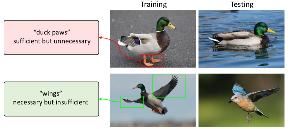
Figure 4: Example for causal sufficiency and necessity in classification problem. The samples on the left are for training and the rights are for tests.

Example of Causal Sufficiency

If the learned representation is represented by the variable $\text{F}_{c}$ (taking binary values 1 or 0), we use it to predict the label of whether being “duck”. If the learned representation contains the information of “duck paws”, it is the sufficient but unnecessary cause because the MML data contains “duck paws” must have a “duck”. However, a sample with“duck” might not contain “duck paws”, e.g., duck swim in the lake. Assuming that $P(\text{Y}_{do({\text{F}_{c}}=1)}=1)=1$ and $P(\text{Y}_{do(\text{F}_{c}=0)}=0)=0.5$, $P(\text{Y}=1)=0.75$, $P(\text{F}_{c}=1,\text{Y}=1)=0.5,P(\text{F}_{c}=0,\text{Y}=0)=0.25,P(\text{F}_{c}=0,\text{Y}=1)=0.25$. Then, following [46], for the probability of sufficiency and necessity, we obtain:

$$\begin{split}\left\{\begin{matrix}P(\text{Y}_{do(\text{F}_{c}=1)}=1|\text{Y}=0,\text{F}_{c}=0)=\frac{P(\text{Y}_{do({\text{F}_{c}}=1)}=1)-P(\text{Y}=1)}{P(\text{Y}=0,\text{F}_{c}=0)}=\frac{1-0.75}{P(\text{Y}=1,\text{F}_{c}=1)}=1\\[8.0pt] P(\text{Y}_{do(\text{F}_{c}=0)}=0|\text{Y}=1,\text{F}_{c}=1)=\frac{P(\text{Y}=1)-P(\text{Y}_{do({\text{F}_{c}}=0)}=1)}{P(\text{Y}=1,\text{F}_{c}=1)}=\frac{0.75-0.5}{P(\text{Y}=1,\text{F}_{c}=1)}=0.5\end{matrix}\right.\end{split}$$ (52)

where the first line represents the probability of sufficiency and the second line represents the probability of necessity. Thus, the learned representation contains “laugh (positive)-good (positive)-rising tone (positive)” has a probability of being the sufficient but unnecessary cause.

Example of Causal Necessity

If the learned representation contains the information of “wings” $\text{F}_{c}$ (taking values 1 and 0, where 1 means “wings”), to predict Y (“duck” 1, other label 0). Since a “duck” must have “wings” but if give a sample with “bird”, it may also have “wings”. Assuming that $P(\text{Y}_{do(\text{F}_{c}=1)}=1)=0.5$ and $P(\text{Y}_{do(\text{F}_{c}=0)}=0)=1$, $P(\text{Y}=1)=0.25$, $P(\text{F}_{c}=1,\text{Y}=1)=0.25,P(\text{F}_{c}=0,\text{Y}=0)=0.5,P(\text{F}_{c}=0,\text{Y}=1)=0.25$. Then, for the probability of sufficiency and necessity, we obtain:

$$\begin{split}\left\{\begin{matrix}P(\text{Y}_{do({\text{F}_{c}}=1)}=1|\text{Y}=0,\text{F}_{c}=0)=\frac{P(\text{Y}_{do({\text{F}_{c}}=1)}=1)-P(\text{Y}=1)}{P(\text{Y}=0,\text{F}_{c}=0)}=0.5\\[8.0pt] P(\text{Y}_{do({\text{F}_{c}}=0)}=0|\text{Y}=1,\text{F}_{c}=1)=\frac{P(\text{Y}=1)-P(\text{Y}_{do({\text{F}_{c}}=0)}=1)}{P(\text{Y}=1,\text{F}_{c}=1)}=1\end{matrix}\right.\end{split}$$ (53)

where the first line represents the probability of sufficiency and the second line represents the probability of necessity. Thus, the learned representation has a probability of being the necessary but insufficient cause.

If we only focus on causal sufficient causes, we will lose important modality-specific information and affect generalizability; if we only focus on causal necessary causes, then decisions will be made incorrectly based on background knowledge, affecting discriminability. For sufficient and necessary causes, the probability of sufficiency or necessity should both be 1. Together they ensure that the MML model can learn a representation that not only reflects different modal information, i.e., contains the semantics of all three modalities, but also targets primary events, i.e., the “duck” label.

Appendix C Benchmark Datasets

In this section, we briefly introduce all datasets used in our experiments. In summary, the benchmark datasets can be divided into four categories: (i) scenes recognition on two datasets, i.e., NYU Depth V2 [51] and SUN RGBD [52] datasets, with two modalities, i.e., RGB and depth images; (ii) image-text classification on two datasets, i.e., UPMC FOOD101 [59] and MVSA [45] datasets, with two modalities, i.e., image and text; (iii) segmentation when consider missing modalities on the BraTS dataset [43, 5] with four modalities, i.e., Flair, T1, T1c, and T2; and (iv) MMLSynData mentioned in Appendix B.1 which is an MML synthetic dataset that used to evaluate whether learned representations contain causal sufficiency and necessity. The composition of the data set is as follows:

• NYU Depth V2 [51] is an indoor scene dataset captured by New York University using Microsoft Kinect’s RGB and depth cameras. It includes 1,449 labeled RGB and depth images across 464 distinct indoor scenes from three cities, along with 407,024 unlabeled images.

• SUN RGBD [52] is a scene understanding dataset released by the Vision & Robotics Group at Princeton University. It comprises 10,335 RGB-D images of indoor scenes, which are pairs of color and depth images. These images were captured using four different types of 3D cameras, including the Intel RealSense, Asus Xtion, Kinect v1, and Kinect v2. Each image in the dataset has been meticulously annotated with 2D polygonal segmentation and 3D bounding boxes.

• UPMC FOOD101 [59] is a comprehensive food recognition dataset consisting of 101,000 images across 101 categories. Each category features 750 training images and 250 test images. Notably, the images are stored in JPEG format and are uniformly resized to a maximum dimension of 512 pixels.

• MVSA [45] is a multimodal biometric dataset that includes a variety of biometric samples such as fingerprints, iris, face, and hand shapes. It is designed to support research in the fields of biometric recognition and security applications. The MVSA dataset typically comprises a rich collection of samples with image and text modalities.

• BraTS [43, 5] aims to segment specific areas within brain tumors, which are identified as the enhancing tumor (ET), the tumor core (TC), and the entire tumor (WT). The dataset is composed of 3D multi-modal MRI scans of the brain, featuring modalities such as Flair (Fl), T1, T1 contrast-enhanced (T1c), and T2, all of which come with corresponding ground-truth segmentations. It includes a training set of 285 cases and an evaluation set of 66 cases. While the ground-truth annotations for the training cases are accessible to the public, those for the validation set remain undisclosed.

• MMLSynData aims to analyze whether the learned representations contain causal sufficiency and necessity. It contains four types of data, i.e., sufficient and necessary causes (SNC), sufficient but unnecessary causes (SC), necessary but insufficient causes (NC), and spurious correlations (SP). Each type of data uses 250 MML samples for training and 50 groups for evaluation. The construction details and corresponding functions are described in Appendix B.1.

Appendix D Baselines

For comprehensive evaluation of the proposed $C^{3}$R, we select 5 types of comparison baselines for evaluation, which covers almost all types of MML baselines including (i) large model and foundation model for MML, i.e., CLIP [53], ALIGN [24], CoOp [25], MaPLe [31], and VPT [25]; (ii) classic MML methods, i.e., RGB [69], Depth [69], Late fusion [56], ConcatMML [72], and AlignMML [56]; (iii) strong unimodal baselines and the corresponding multi-modal methods, i.e., Bow [69], Img [69], BERT [69], ConcatBow [69], and ConcatBERT [69]; (iv) recently proposed and SOTA MML methods, i.e., MMTM [30] and TMC [20], LCKD [55], UniCODE [63], SimMMDG [13], MMBT [32], and QMF [69]; and (v) MML methods that specifically designed for missing modalities, i.e., HMIS [21], HVED [14], RSeg [9], mmFm [71], and LCKD [55].

Appendix E Implementation Details

For the model architecture, we use a three-layer Multilayer Perceptron (MLP) neural network with activation functions designed following [10] as the causal representations learner. The dimensions of the hidden vectors of each layer are specified as 64, 32, and 128, while the learned representation is 64. We embed this network into MML models or introduce a classifier to predict labels. For the basic MML model, we follow the commonly used structure mentioned in [70, 64].

Moving on to the optimization process, we employ the Adam optimizer to train our model. Momentum and weight decay are set at $0.8$ and $10^{-4}$, respectively. The initial learning rate for all experiments is established at 0.1, with the flexibility for linear scaling as required. Additionally, we use grid search to set the hyperparameters $\lambda_{1}=0.01$, $\lambda_{2}=0.55$, and $\lambda_{3}=0.4$. Note that we specially construct corresponding ablation experiments for the selection of these parameters, as described in Appendix F. Experimental results show that the model can maintain relatively stable performance on various data sets using different hyperparameter settings.

For evaluation, the training dataset is randomly split as training and validation datasets, the hyperparameters are selected on the validation dataset, which maximizes the performance of the validation dataset. The overall accuracy results are evaluated on the test dataset rather than the validation dataset. All experimental procedures are executed using NVIDIA RTX A6000 GPUs, and all experimental results are obtained on the basis of five rounds of experiments.

Table 4: Full results (with error bars) of scenes recognition performance on NYU Depth V2 [51] and SUN RGBD [52] with RGB and depth images. “(N, Avg.)” and “(N, Worst.)” denotes the average and worst-case accuracy. The results show the error of accuracy by executing the experiments randomly 3 times on 40 randomly selected hyperparameters. The best results are highlighted in bold.

Method	NYU Depth V2				SUN RGB-D
	(0,Avg.)	(0,Worst.)	(10,Avg.)	(10,Worst.)	(0,Avg.)	(0,Worst.)	(10,Avg.)	(10,Worst.)
CLIP [53]	69.32$\pm$0.35	68.29$\pm$0.36	51.67$\pm$0.42	48.54$\pm$0.36	56.24$\pm$0.51	54.73$\pm$0.31	35.65$\pm$0.47	32.76$\pm$0.54
ALIGN [24]	66.43$\pm$0.36	64.33$\pm$0.32	45.24$\pm$0.47	42.42$\pm$0.38	57.32$\pm$0.52	56.26$\pm$0.36	38.43$\pm$0.42	35.13$\pm$0.52
MaPLe [31]	71.26$\pm$0.32	69.27$\pm$0.35	52.98$\pm$0.45	48.73$\pm$0.37	62.44$\pm$0.54	61.76$\pm$0.33	34.51$\pm$0.42	30.29$\pm$0.54
CoOp [25]	67.48$\pm$0.34	66.94$\pm$0.32	49.43$\pm$0.44	45.62$\pm$0.32	58.36$\pm$0.50	56.31$\pm$0.36	39.67$\pm$0.41	35.43$\pm$0.55
VPT [25]	62.16$\pm$0.36	61.21$\pm$0.31	41.05$\pm$0.47	37.81$\pm$0.32	54.72$\pm$0.54	53.92$\pm$0.32	33.48$\pm$0.44	29.81$\pm$0.51
RGB [69]	63.33$\pm$0.35	62.54$\pm$0.32	45.46$\pm$0.47	42.20$\pm$0.38	56.78$\pm$0.51	56.51$\pm$0.36	42.94$\pm$0.45	41.02$\pm$0.54
Depth [69]	62.65$\pm$0.37	61.01$\pm$0.34	44.13$\pm$0.48	35.93$\pm$0.32	52.99$\pm$0.55	51.32$\pm$0.32	35.63$\pm$0.40	33.07$\pm$0.54
Late fusion [56]	69.14$\pm$0.33	68.35$\pm$0.32	51.99$\pm$0.49	44.95$\pm$0.32	62.09$\pm$0.58	60.55$\pm$0.38	47.33$\pm$0.46	44.60$\pm$0.57
ConcatMML [72]	70.30$\pm$0.32	69.42$\pm$0.36	53.20$\pm$0.47	47.71$\pm$0.31	61.90$\pm$0.52	61.19$\pm$0.37	45.64$\pm$0.41	42.95$\pm$0.50
AlignMML [56]	70.31$\pm$0.36	68.50$\pm$0.37	51.74$\pm$0.42	44.19$\pm$0.39	61.12$\pm$0.52	60.12$\pm$0.33	44.19$\pm$0.47	38.12$\pm$0.51
Bow [69]	61.38$\pm$0.35	59.23$\pm$0.36	37.98$\pm$0.42	34.24$\pm$0.38	54.37$\pm$0.50	54.11$\pm$0.34	39.07$\pm$0.47	36.43$\pm$0.53
Img [69]	43.27$\pm$0.33	42.96$\pm$0.34	29.27$\pm$0.46	28.53$\pm$0.37	36.28$\pm$0.54	35.26$\pm$0.36	21.32$\pm$0.40	20.31$\pm$0.53
BERT [69]	65.31$\pm$0.36	63.23$\pm$0.32	38.64$\pm$0.47	36.45$\pm$0.33	57.98$\pm$0.52	56.74$\pm$0.35	42.51$\pm$0.41	38.53$\pm$0.57
ConcatBow [69]	49.64$\pm$0.36	48.66$\pm$0.34	31.43$\pm$0.45	29.87$\pm$0.30	41.25$\pm$0.54	40.54$\pm$0.32	26.76$\pm$0.49	24.27$\pm$0.58
ConcatBERT [69]	70.56$\pm$0.34	69.83$\pm$0.36	44.52$\pm$0.46	43.29$\pm$0.34	59.76$\pm$0.52	58.92$\pm$0.34	45.85$\pm$0.42	41.76$\pm$0.54
MMTM [30]	71.04$\pm$0.36	70.18$\pm$0.34	52.28$\pm$0.42	46.18$\pm$0.33	61.72$\pm$0.56	60.94$\pm$0.31	46.03$\pm$0.44	44.28$\pm$0.57
TMC [20]	71.06$\pm$0.34	69.57$\pm$0.32	53.36$\pm$0.42	49.23$\pm$0.39	60.68$\pm$0.54	60.31$\pm$0.30	45.66$\pm$0.46	41.60$\pm$0.50
LCKD [55]	68.01$\pm$0.31	66.15$\pm$0.34	42.31$\pm$0.45	40.56$\pm$0.38	56.43$\pm$0.56	56.32$\pm$0.32	43.21$\pm$0.49	42.43$\pm$0.54
UniCODE [63]	70.12$\pm$0.37	68.74$\pm$0.32	44.78$\pm$0.48	42.79$\pm$0.39	59.21$\pm$0.55	58.55$\pm$0.36	46.32$\pm$0.47	42.21$\pm$0.57
SimMMDG [13]	71.34$\pm$0.32	70.29$\pm$0.31	45.67$\pm$0.41	44.83$\pm$0.39	60.54$\pm$0.50	60.31$\pm$0.37	47.86$\pm$0.43	45.79$\pm$0.56
MMBT [32]	67.00$\pm$0.35	65.84$\pm$0.34	49.59$\pm$0.41	47.24$\pm$0.38	56.91$\pm$0.51	56.18$\pm$0.36	43.28$\pm$0.47	39.46$\pm$0.51
QMF [69]	70.09$\pm$0.30	68.81$\pm$0.34	55.60$\pm$0.42	51.07$\pm$0.34	62.09$\pm$0.50	61.30$\pm$0.36	48.58$\pm$0.46	47.50$\pm$0.58
CLIP+$C^{3}$R	75.98$\pm$0.33 (+6.66)	74.28$\pm$0.36 (+5.99)	56.32$\pm$0.42 (+4.65)	52.23$\pm$0.36 (+3.69)	61.39$\pm$0.59 (+5.15)	58.17$\pm$0.37 (+3.44)	40.86$\pm$0.46 (+5.21)	37.24$\pm$0.50 (+4.48)
ALIGN+$C^{3}$R	71.28$\pm$0.32 (+4.85)	69.75$\pm$0.38 (+5.42)	51.63$\pm$0.46 (+6.39)	50.06$\pm$0.38 (+7.64)	62.14$\pm$0.51 (+4.82)	61.24$\pm$0.35 (+4.98)	44.76$\pm$0.40 (+6.33)	41.52$\pm$0.59 (+6.39)
MaPLe+$C^{3}$R	76.21$\pm$0.30 (+4.95)	73.54$\pm$0.32 (+4.27)	58.26$\pm$0.49 (+5.28)	54.91$\pm$0.37 (+6.18)	64.86$\pm$0.50 (+2.42)	64.63$\pm$0.35 (+2.87)	39.04$\pm$0.43 (+4.53)	36.82$\pm$0.51 (+6.53)
Late fusion+$C^{3}$R	72.57$\pm$0.36 (+3.43)	71.23$\pm$0.38 (+2.88)	56.78$\pm$0.42 (+4.79)	49.84$\pm$0.37 (+4.89)	64.15$\pm$0.56 (+2.06)	62.31$\pm$0.38 (+1.76)	52.96$\pm$0.42 (+5.63)	49.37$\pm$0.54 (+4.77)
ConcatMML+$C^{3}$R	74.76$\pm$0.30 (+4.46)	75.37$\pm$0.32 (+5.95)	59.37$\pm$0.48 (+6.17)	54.55$\pm$0.36 (+6.84)	66.54$\pm$0.57 (+4.64)	65.82$\pm$0.39 (+4.63)	51.24$\pm$0.44 (+5.60)	49.85$\pm$0.54 (+6.90)
Bow+$C^{3}$R	65.23$\pm$0.39 (+3.85)	64.14$\pm$0.34 (+4.91)	43.58$\pm$0.40 (+5.60)	42.21$\pm$0.37 (+7.97)	58.26$\pm$0.52 (+3.89)	57.23$\pm$0.38 (+3.12)	46.71$\pm$0.45 (+7.64)	42.96$\pm$0.53 (+6.53)
LCKD+$C^{3}$R	75.83$\pm$0.31 (+7.82)	73.84$\pm$0.34 (+7.69)	48.95$\pm$0.43 (+6.64)	47.31$\pm$0.32 (+6.75)	60.11$\pm$0.54 (+3.68)	59.65$\pm$0.30 (+3.33)	45.99$\pm$0.41 (+2.78)	45.13$\pm$0.57 (+2.70)
UniCODE+$C^{3}$R	75.45$\pm$0.35 (+5.33)	73.02$\pm$0.33 (+4.28)	50.55$\pm$0.45 (+5.77)	47.34$\pm$0.30 (+4.55)	64.89$\pm$0.55 (+5.68)	63.20$\pm$0.34 (+4.65)	50.36$\pm$0.46 (+4.04)	48.56$\pm$0.52 (+6.35)
SimMMDG+$C^{3}$R	74.39$\pm$0.36 (+3.05)	73.98$\pm$0.37 (+3.69)	49.15$\pm$0.40 (+3.48)	46.22$\pm$0.34 (+1.39)	64.34$\pm$0.50 (+3.80)	63.50$\pm$0.36 (+3.19)	51.54$\pm$0.42 (+3.68)	51.01$\pm$0.52 (+5.22)
MMBT+$C^{3}$R	72.87$\pm$0.39 (+5.87)	70.93$\pm$0.33 (+5.09)	53.29$\pm$0.45 (+3.70)	51.30$\pm$0.31 (+4.06)	60.32$\pm$0.52 (+3.41)	59.18$\pm$0.34 (+3.00)	47.89$\pm$0.48 (+4.61)	45.19$\pm$0.56 (+5.73)
QMF+$C^{3}$R	76.56$\pm$0.35 (+6.47)	74.01$\pm$0.38 (+5.20)	58.54$\pm$0.42 (+2.94)	58.13$\pm$0.30 (+7.06)	66.77$\pm$0.54 (+4.68)	64.90$\pm$0.32 (+3.60)	51.15$\pm$0.48 (+2.57)	50.00$\pm$0.55 (+2.50)

Table 5: Full results (with error bars) of image-text classification performance on UPMC FOOD101 [59] and MVSA [45] with image and text. “(N, Avg.)” and “(N, Worst.)” denotes the average and worst-case accuracy. The results show the error of accuracy by executing the experiments randomly 3 times on 40 randomly selected hyperparameters. The best results are highlighted in bold.

Method	FOOD 101				MVSA
	(0,Avg.)	(0,Worst.)	(10,Avg.)	(10,Worst.)	(0,Avg.)	(0,Worst.)	(10,Avg.)	(10,Worst.)
CLIP [53]	85.24$\pm$0.31	84.20$\pm$0.34	52.12$\pm$0.54	49.31$\pm$0.43	62.48$\pm$0.33	61.22$\pm$0.37	31.64$\pm$0.58	28.27$\pm$0.54
ALIGN [24]	86.14$\pm$0.32	85.00$\pm$0.33	53.21$\pm$0.52	50.85$\pm$0.47	63.25$\pm$0.36	62.69$\pm$0.32	30.55$\pm$0.56	26.44$\pm$0.59
MaPLe [31]	90.40$\pm$0.32	86.28$\pm$0.37	53.16$\pm$0.56	40.21$\pm$0.47	77.43$\pm$0.32	75.36$\pm$0.30	43.72$\pm$0.56	38.82$\pm$0.52
CoOp [25]	88.33$\pm$0.30	85.10$\pm$0.32	55.24$\pm$0.56	51.01$\pm$0.48	74.26$\pm$0.33	73.61$\pm$0.34	42.58$\pm$0.56	37.29$\pm$0.58
VPT [25]	83.89$\pm$0.31	82.00$\pm$0.35	51.44$\pm$0.52	49.01$\pm$0.47	65.87$\pm$0.36	64.98$\pm$0.37	32.79$\pm$0.50	29.21$\pm$0.59
RGB [69]	83.54$\pm$0.30	82.43$\pm$0.37	54.32$\pm$0.56	52.32$\pm$0.45	69.28$\pm$0.32	69.12$\pm$0.31	51.43$\pm$0.55	47.26$\pm$0.54
Depth [69]	81.37$\pm$0.35	81.21$\pm$0.33	46.29$\pm$0.57	43.57$\pm$0.42	67.52$\pm$0.39	66.76$\pm$0.34	43.77$\pm$0.51	38.68$\pm$0.53
Late fusion [56]	90.69$\pm$0.30	90.58$\pm$0.31	58.00$\pm$0.52	55.77$\pm$0.47	76.88$\pm$0.33	74.76$\pm$0.38	55.16$\pm$0.56	47.78$\pm$0.52
ConcatMML [72]	89.43$\pm$0.34	88.79$\pm$0.32	56.02$\pm$0.52	54.33$\pm$0.48	75.42$\pm$0.33	75.33$\pm$0.30	53.42$\pm$0.51	50.47$\pm$0.53
AlignMML [56]	88.26$\pm$0.30	88.11$\pm$0.38	55.47$\pm$0.57	52.76$\pm$0.42	74.91$\pm$0.36	72.97$\pm$0.34	52.71$\pm$0.55	47.03$\pm$0.52
Bow [69]	82.50$\pm$0.36	82.32$\pm$0.34	41.95$\pm$0.54	41.41$\pm$0.48	48.79$\pm$0.34	35.45$\pm$0.32	41.57$\pm$0.50	32.18$\pm$0.53
Img [69]	64.62$\pm$0.32	64.22$\pm$0.39	33.03$\pm$0.58	32.67$\pm$0.47	64.12$\pm$0.37	62.04$\pm$0.36	45.00$\pm$0.56	39.31$\pm$0.50
BERT [69]	86.46$\pm$0.37	86.42$\pm$0.35	43.88$\pm$0.58	43.56$\pm$0.42	75.61$\pm$0.30	74.76$\pm$0.33	47.41$\pm$0.55	45.86$\pm$0.51
ConcatBow [69]	70.77$\pm$0.35	70.68$\pm$0.34	35.68$\pm$0.58	34.92$\pm$0.41	64.09$\pm$0.37	62.04$\pm$0.35	45.40$\pm$0.56	40.95$\pm$0.54
ConcatBERT [69]	88.20$\pm$0.36	87.81$\pm$0.32	49.86$\pm$0.54	47.79$\pm$0.40	65.59$\pm$0.38	64.74$\pm$0.36	46.12$\pm$0.56	41.81$\pm$0.51
MMTM [30]	89.75$\pm$0.35	89.43$\pm$0.39	57.91$\pm$0.52	54.98$\pm$0.46	74.24$\pm$0.38	73.55$\pm$0.34	54.63$\pm$0.50	49.72$\pm$0.56
TMC [20]	89.86$\pm$0.33	89.80$\pm$0.34	61.37$\pm$0.52	61.10$\pm$0.43	74.88$\pm$0.30	71.10$\pm$0.31	60.36$\pm$0.55	53.37$\pm$0.54
LCKD [55]	85.32$\pm$0.36	84.26$\pm$0.34	47.43$\pm$0.52	44.22$\pm$0.43	62.44$\pm$0.30	62.27$\pm$0.34	43.52$\pm$0.59	38.63$\pm$0.54
UniCODE [63]	88.39$\pm$0.36	87.21$\pm$0.35	51.28$\pm$0.52	47.95$\pm$0.41	66.97$\pm$0.39	65.94$\pm$0.33	48.34$\pm$0.58	42.95$\pm$0.54
SimMMDG [13]	89.57$\pm$0.38	88.43$\pm$0.34	52.55$\pm$0.57	50.31$\pm$0.42	67.08$\pm$0.35	66.35$\pm$0.39	49.52$\pm$0.58	44.01$\pm$0.52
MMBT [32]	91.52$\pm$0.37	91.38$\pm$0.36	56.75$\pm$0.55	56.21$\pm$0.40	78.50$\pm$0.34	78.04$\pm$0.39	55.35$\pm$0.52	52.22$\pm$0.57
QMF [69]	92.92$\pm$0.32	92.72$\pm$0.35	62.21$\pm$0.58	61.76$\pm$0.40	78.07$\pm$0.39	76.30$\pm$0.31	61.28$\pm$0.55	57.61$\pm$0.50
CLIP+$C^{3}$R	92.25$\pm$0.36 (+7.01)	90.74$\pm$0.35 (+6.54)	58.91$\pm$0.52 (+6.79)	56.39$\pm$0.46 (+7.08)	68.94$\pm$0.33 (+6.46)	68.15$\pm$0.37 (+6.93)	38.62$\pm$0.56 (+6.98)	34.73$\pm$0.57 (+6.46)
ALIGN+$C^{3}$R	90.32$\pm$0.36 (+4.18)	89.24$\pm$0.32 (+4.24)	57.47$\pm$0.51 (+4.26)	56.61$\pm$0.43 (+5.76)	67.54$\pm$0.34 (+4.29)	66.34$\pm$0.32 (+3.65)	36.57$\pm$0.56 (+6.02)	32.63$\pm$0.51 (+6.19)
MaPLe+$C^{3}$R	93.71$\pm$0.32 (+3.31)	92.26$\pm$0.30 (+5.98)	59.57$\pm$0.53 (+6.41)	45.83$\pm$0.45 (+5.62)	81.03$\pm$0.34 (+3.60)	80.93$\pm$0.36 (+5.57)	48.95$\pm$0.53 (+5.23)	45.31$\pm$0.57 (+6.49)
Late fusion+$C^{3}$R	93.66$\pm$0.37 (+2.97)	92.05$\pm$0.38 (+1.47)	64.32$\pm$0.56 (+6.32)	58.61$\pm$0.42 (+2.84)	83.44$\pm$0.33 (+6.56)	79.28$\pm$0.34 (+4.52)	61.86$\pm$0.50 (+6.70)	52.08$\pm$0.56 (+4.30)
ConcatMML+$C^{3}$R	94.12$\pm$0.37 (+4.69)	93.52$\pm$0.36 (+4.73)	60.22$\pm$0.54 (+4.20)	58.73$\pm$0.43 (+4.40)	79.66$\pm$0.39 (+4.24)	78.23$\pm$0.37 (+2.90)	58.42$\pm$0.54 (+5.00)	57.12$\pm$0.50 (+6.65)
Bow+$C^{3}$R	85.68$\pm$0.36 (+3.18)	89.16$\pm$0.37 (+6.84)	46.07$\pm$0.50 (+4.12)	47.98$\pm$0.42 (+6.57)	54.27$\pm$0.38 (+5.48)	42.64$\pm$0.31 (+7.19)	47.38$\pm$0.52 (+5.81)	37.53$\pm$0.57 (+5.35)
LCKD+$C^{3}$R	90.01$\pm$0.34 (+4.69)	89.23$\pm$0.38 (+4.97)	53.84$\pm$0.57 (+6.41)	50.77$\pm$0.41 (+6.55)	66.41$\pm$0.30 (+3.97)	65.06$\pm$0.33 (+2.79)	48.45$\pm$0.58 (+4.93)	42.00$\pm$0.51 (+3.37)
UniCODE+$C^{3}$R	91.40$\pm$0.33 (+3.01)	89.15$\pm$0.37 (+1.94)	54.66$\pm$0.50 (+3.38)	51.90$\pm$0.44 (+3.95)	70.07$\pm$0.39 (+3.10)	67.32$\pm$0.36 (+1.38)	51.98$\pm$0.52 (+3.64)	47.28$\pm$0.56 (+4.33)
SimMMDG+$C^{3}$R	91.55$\pm$0.38 (+1.98)	90.12$\pm$0.34 (+1.69)	56.38$\pm$0.59 (+3.83)	53.15$\pm$0.43 (+2.84)	72.77$\pm$0.37 (+5.69)	70.42$\pm$0.35 (+4.07)	51.36$\pm$0.51 (+1.84)	50.88$\pm$0.55 (+6.87)
MMBT+$C^{3}$R	93.89$\pm$0.36 (+2.37)	93.22$\pm$0.34 (+1.84)	60.23$\pm$0.53 (+3.48)	59.55$\pm$0.45 (+3.34)	82.64$\pm$0.38 (+4.14)	81.27$\pm$0.31 (+3.23)	61.81$\pm$0.50 (+6.46)	58.19$\pm$0.56 (+5.97)
QMF+$C^{3}$R	94.25$\pm$0.38 (+1.33)	93.41$\pm$0.30 (+0.69)	65.33$\pm$0.51 (+3.12)	62.74$\pm$0.43 (+0.98)	82.56$\pm$0.37 (+4.49)	81.37$\pm$0.33 (+5.07)	66.37$\pm$0.52 (+5.09)	64.02$\pm$0.59 (+6.41)

Appendix F Full Results and Additional Experiments

In this section, we provide the full results and analyses of the experiments in Section 6 and additional experiments which can only be supplemented in the appendix due to space limitations. Specifically, we first provide full results and additional details of “Performance and Robustness Analysis” (the first experiment in Section 6.2 with Table 1), including performance on all MML baseline methods and more analysis conclusions (Appendix F.1). Then, we provide the additional details and analysis of “When faces the problem of missing modalities” (the second experiment in Section 6.2 with Table 2). Next, we provide the full results and more analysis of “Learning causal complete representations” (the third experiment in Section 6.2 with Figure 3), including the detailed settings, the visualization and more analysis of the correlation between different methods and different causal causes under different spurious degrees. Finally, we provide the full results and additional experiments of the ablation study, including the experiments about model efficiency, trade-off performance, and parameter sensitivity.

F.1 Full Results and Additional Details of Performance and Robustness Analysis

Due to space limitations, we provide part of the experimental results in Table 1 of the main text, which contains typical methods of all categories of baselines mentioned in Appendix D. In Table 4 and Table 5, we provide comparison baselines for all baselines. Specifically, Table 4 provides the experiments about scene recognition on NYU Depth V2 [51] and SUN RGBD [52] datasets. Table 5 provides the experiments about image-text classification on UPMC FOOD101 [59] and MVSA [45] datasets. From the results, we can observe that (i) $C^{3}$R achieves stable improvements in both the average and worst-case accuracy on almost all the comparison baselines, including both the foundation model and all types of MML baselines; and (ii) regardless of the data scale, $C^{3}$R can bring obvious and stable performance improvements, with an average increase of more than 5%.. This proves the superior effect and robustness of $C^{3}$R.

F.2 Full Results and Additional Details of Performance with Missing Modalities

Due to the complexity of data in real systems, MML methods face the dilemma of missing modalities [73, 66]. This problem severely affects model performance, especially when important modes are missing. Therefore, in order for the model to have good practicality, it is very critical to be able to maintain stable performance in the face of missing modes. To evaluate the performance of the proposed $C^{3}$R when facing missing modalities, we constructed comparative experiments on all 15 possible combinations of missing modalities on BraTS. Specifically, based on BraTS, we construct fifteen combinations of different modes following [55]. Then, we recorded the performance of $C^{3}$R and several strong baseline models after five runs.

From the results illustrated in Table 2, we can observe that (i) using F1 and T1c, the model performs much better than others on Enhancing Tumour. Likewise, T1c and Flair from the Tumour Core and Whole Tumour contributed the most. (ii) The model has been significantly improved after the introduction of $C^{3}$R, especially when important modes are missing, e.g., F1 on Enhancing Tumour. The results prove that our method can improve the performance of the model in the scenario of missing modality and improve the stability.

F.3 Full Results and Additional Details of Causal Complete Evaluation

In order to verify whether our method $C^{3}$R actually extracts causal necessary and sufficient representations, we construct a synthetic data set called MMLSynData (as mentioned in Appendix B.1) to conduct comparative experiments. Specifically, we first built MMLSynData, which is a synthetic data set for MML scenarios containing four types of data, i.e., sufficient and necessary causes (SNC), sufficient but unnecessary causes (SC), necessary but insufficient causes (NC), and spurious correlations (SP). Each category contains 250 sets of training data and 50 sets of test data. Next, based on the above 1200 sets of data, we set different degrees of spurious correlation $D_{sp}$ for comparative experiments, including $D_{sp}=0.3$ and $D_{sp}=0.6$. It is worth noting that the result shown in Figure 3 in the text is $D_{sp}=0.6$. Then, we choose SOTA and classic MML methods to compare with the basic MML framework after the introduction of $C^{3}$R, where $basic$ represents a simple MML learning framework based on the Conv4 backbone network and a classifier following [56]. We record their correlation with four different types of data in MMLSynData.

The results of $D_{sp}=0.3$ and $D_{sp}=0.6$ (also the results shown in Figure 3) are shown in Figure 5. Combined with Figure 3, the results show that compared with other methods, the correlation with real data (such as SN, SF, and NC) is higher after the introduction of $C^{3}$R, and the correlation with spurious correlation (SP ) has a lower score. For example, when $D_{sp}=0.3$, we obtain the average distance correlations of SNC, SC, NC, and SP as 0.91, 0.71, 0.69, 0.13 respectively. Furthermore, when we set $D_{sp}$ to a larger value of 0.6, the distance correlation between the MML method and false information is almost unchanged after introducing $C^{3}$R, while other methods are difficult to achieve this. The results show that when there are more spurious correlations in the data, $C^{3}$R still tends to capture valid information from the real data to extract sufficient and necessary causes.

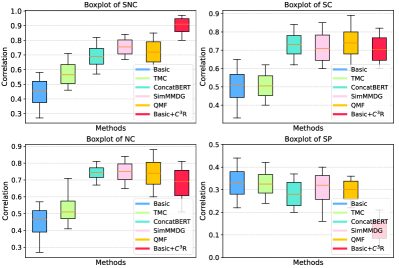
(a) Spurious correlation degree $D_{sp}=0.3$

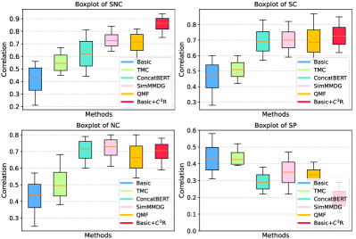
(b) Spurious correlation degree $D_{sp}=0.6$

Figure 5: Evaluation for the property of learned representations (identification for SNC, SC, NC, and SP) with different spurious correlation degree $D_{sp}$.

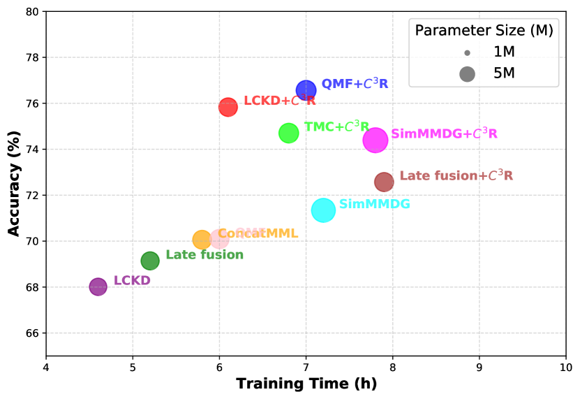
Figure 6: Trade-off Performance of different methods on (0,Avg.) NYU Depth V2.

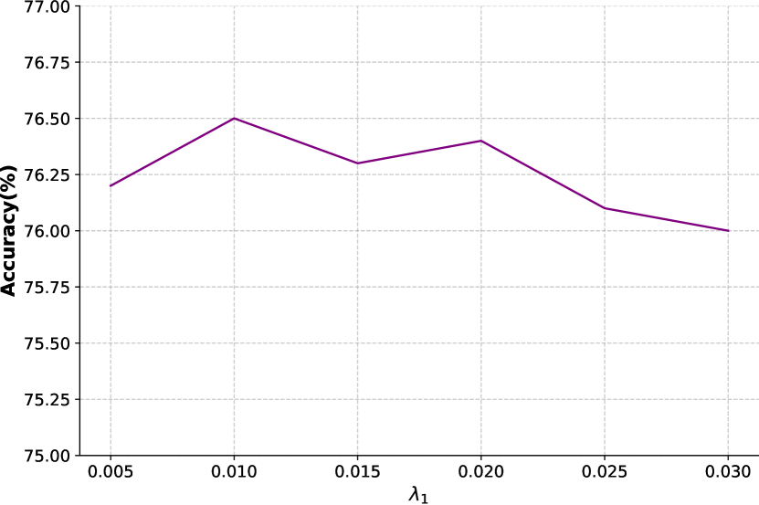
Figure 7: Parameter sensitivity about $\lambda_{1}$ on (0,Avg.) NYU Depth V2.

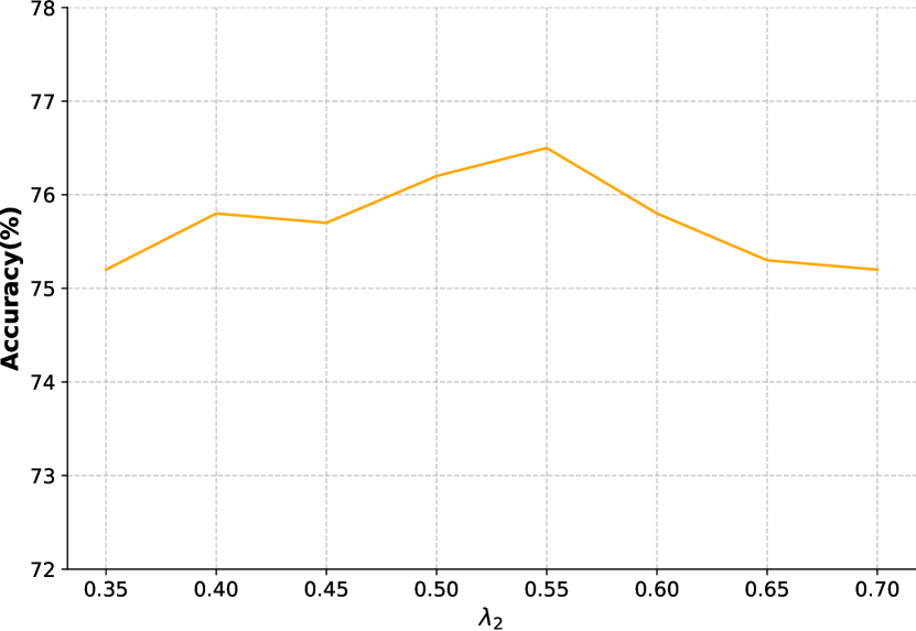
Figure 8: Parameter sensitivity about $\lambda_{2}$ on (0,Avg.) NYU Depth V2.

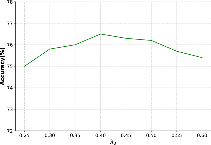
Figure 9: Parameter sensitivity about $\lambda_{3}$ on (0,Avg.) NYU Depth V2.

F.4 Full Results and Additional Details of Ablation Study

To evaluate the effect of the model and understand how $C^{3}$R works well, we constructed a series of experiments, including (i) the effect of each item in the $C^{3}$R objective (Eq.14) as shown in Section 6.2; (ii) trade-off performance about the model efficiency and accuracy after introducing $C^{3}$R; (iii) parameter sensitivity about the three hyperparameters in the $C^{3}$R objective (Eq.14), i.e., $\lambda_{1}$, $\lambda_{2}$, and $\lambda_{3}.$. In this section, we provide details about the latter two experiments and results, where the results of the first experiment are shown in Figure 3.

Model efficiency

Since $C^{3}$R is a plug-and-play module, in order to ensure its practicability, we explore the balance between model performance and efficiency. We compare the trade-off performance of multiple baselines before and after using our $C^{3}$R with the same Conv4 backbone. The results illustrated in Figure 7 show that introducing $C^{3}$R achieves great performance with acceptable computational cost.

Parameter sensitivity

We determine the hyperparameters of the regularization term in the experiment based on the performance of the validation samples. Specifically, for each experimental scenario, we test the impact of different values of $\lambda_{1}$, $\lambda_{2}$ and $\lambda_{3}$ on model performance. The range of these values is set between $\left[0.001,0.5\right]$. In each scenario, we first use grid search to screen the parameters with a difference of 0.1. After screening the optimal interval, we screened the parameters with a difference of 0.01 and recorded the final average results.

The results are shown in Figures 7-9. From the results, we observe that when $\lambda_{1}=0.01$, $\lambda_{2}=0.55$, and $\lambda_{3}=0.4$, the results are better which is also our choice. Meanwhile, the model effect does not change significantly under different parameters, which illustrates the stability of the parameters and the convenience of adjustment in reality.

NeurIPS Paper Checklist

1. Claims

2. Question: Do the main claims made in the abstract and introduction accurately reflect the paper’s contributions and scope?

3. Answer: [Yes]

4. Justification: The main contribution of this paper is to explore and ensure the causal sufficiency and necessity of the learned representation for MML, effectively improving the MML performance. This has been discussed in the abstract and introduction.

5. Guidelines:

   • The answer NA means that the abstract and introduction do not include the claims made in the paper.

   • The abstract and/or introduction should clearly state the claims made, including the contributions made in the paper and important assumptions and limitations. A No or NA answer to this question will not be perceived well by the reviewers.

   • The claims made should match theoretical and experimental results, and reflect how much the results can be expected to generalize to other settings.

   • It is fine to include aspirational goals as motivation as long as it is clear that these goals are not attained by the paper.

6. Limitations

7. Question: Does the paper discuss the limitations of the work performed by the authors?

8. Answer: [Yes]

9. Justification: We’ve clearly stated the limitations and future directions to improve this work in Conclusion section.

10. Guidelines:

    • The answer NA means that the paper has no limitation while the answer No means that the paper has limitations, but those are not discussed in the paper.

    • The authors are encouraged to create a separate "Limitations" section in their paper.

    • The paper should point out any strong assumptions and how robust the results are to violations of these assumptions (e.g., independence assumptions, noiseless settings, model well-specification, asymptotic approximations only holding locally). The authors should reflect on how these assumptions might be violated in practice and what the implications would be.

    • The authors should reflect on the scope of the claims made, e.g., if the approach was only tested on a few datasets or with a few runs. In general, empirical results often depend on implicit assumptions, which should be articulated.

    • The authors should reflect on the factors that influence the performance of the approach. For example, a facial recognition algorithm may perform poorly when image resolution is low or images are taken in low lighting. Or a speech-to-text system might not be used reliably to provide closed captions for online lectures because it fails to handle technical jargon.

    • The authors should discuss the computational efficiency of the proposed algorithms and how they scale with dataset size.

    • If applicable, the authors should discuss possible limitations of their approach to address problems of privacy and fairness.

    • While the authors might fear that complete honesty about limitations might be used by reviewers as grounds for rejection, a worse outcome might be that reviewers discover limitations that aren’t acknowledged in the paper. The authors should use their best judgment and recognize that individual actions in favor of transparency play an important role in developing norms that preserve the integrity of the community. Reviewers will be specifically instructed to not penalize honesty concerning limitations.

11. Theory Assumptions and Proofs

12. Question: For each theoretical result, does the paper provide the full set of assumptions and a complete (and correct) proof?

13. Answer: [Yes]

14. Justification: We state the assumption of each theorem and proposition in the corresponding location, e.g., Assumption 3.5. Meanwhile, We provide constraints for the assumption of exogeneity and monotonicity. All the proofs are provided in Appendix A. We also highlight the locations of corresponding proofs in the main text.

15. Guidelines:

    • The answer NA means that the paper does not include theoretical results.

    • All the theorems, formulas, and proofs in the paper should be numbered and cross-referenced.

    • All assumptions should be clearly stated or referenced in the statement of any theorems.

    • The proofs can either appear in the main paper or the supplemental material, but if they appear in the supplemental material, the authors are encouraged to provide a short proof sketch to provide intuition.

    • Inversely, any informal proof provided in the core of the paper should be complemented by formal proofs provided in appendix or supplemental material.

    • Theorems and Lemmas that the proof relies upon should be properly referenced.

16. Experimental Result Reproducibility

17. Question: Does the paper fully disclose all the information needed to reproduce the main experimental results of the paper to the extent that it affects the main claims and/or conclusions of the paper (regardless of whether the code and data are provided or not)?

18. Answer: [Yes]

19. Justification: We have provided all the code, data, and instructions in the supplemental material. We also have provided all the implementation details, the total amount of compute and the type of resources used in Section 6.1, Appendix E, and the locations of each experiment (Section 6 and Appendix).

20. Guidelines:

    • The answer NA means that the paper does not include experiments.

    • If the paper includes experiments, a No answer to this question will not be perceived well by the reviewers: Making the paper reproducible is important, regardless of whether the code and data are provided or not.

    • If the contribution is a dataset and/or model, the authors should describe the steps taken to make their results reproducible or verifiable.

    • Depending on the contribution, reproducibility can be accomplished in various ways. For example, if the contribution is a novel architecture, describing the architecture fully might suffice, or if the contribution is a specific model and empirical evaluation, it may be necessary to either make it possible for others to replicate the model with the same dataset, or provide access to the model. In general. releasing code and data is often one good way to accomplish this, but reproducibility can also be provided via detailed instructions for how to replicate the results, access to a hosted model (e.g., in the case of a large language model), releasing of a model checkpoint, or other means that are appropriate to the research performed.

    • While NeurIPS does not require releasing code, the conference does require all submissions to provide some reasonable avenue for reproducibility, which may depend on the nature of the contribution. For example

      1. If the contribution is primarily a new algorithm, the paper should make it clear how to reproduce that algorithm.

      2. If the contribution is primarily a new model architecture, the paper should describe the architecture clearly and fully.

      3. If the contribution is a new model (e.g., a large language model), then there should either be a way to access this model for reproducing the results or a way to reproduce the model (e.g., with an open-source dataset or instructions for how to construct the dataset).

      4. We recognize that reproducibility may be tricky in some cases, in which case authors are welcome to describe the particular way they provide for reproducibility. In the case of closed-source models, it may be that access to the model is limited in some way (e.g., to registered users), but it should be possible for other researchers to have some path to reproducing or verifying the results.

21. Open access to data and code

22. Question: Does the paper provide open access to the data and code, with sufficient instructions to faithfully reproduce the main experimental results, as described in supplemental material?

23. Answer: [Yes]

24. Justification: We have provided the code, data, instructions, etc. which are needed to reproduce the main experimental results in the supplemental material.

25. Guidelines:

    • The answer NA means that paper does not include experiments requiring code.

    • Please see the NeurIPS code and data submission guidelines (https://nips.cc/public/guides/CodeSubmissionPolicy) for more details.

    • While we encourage the release of code and data, we understand that this might not be possible, so “No” is an acceptable answer. Papers cannot be rejected simply for not including code, unless this is central to the contribution (e.g., for a new open-source benchmark).

    • The instructions should contain the exact command and environment needed to run to reproduce the results. See the NeurIPS code and data submission guidelines (https://nips.cc/public/guides/CodeSubmissionPolicy) for more details.

    • The authors should provide instructions on data access and preparation, including how to access the raw data, preprocessed data, intermediate data, and generated data, etc.

    • The authors should provide scripts to reproduce all experimental results for the new proposed method and baselines. If only a subset of experiments are reproducible, they should state which ones are omitted from the script and why.

    • At submission time, to preserve anonymity, the authors should release anonymized versions (if applicable).

    • Providing as much information as possible in supplemental material (appended to the paper) is recommended, but including URLs to data and code is permitted.

26. Experimental Setting/Details

27. Question: Does the paper specify all the training and test details (e.g., data splits, hyperparameters, how they were chosen, type of optimizer, etc.) necessary to understand the results?

28. Answer: [Yes]

29. Justification: We have provided all the training and test details, e.g., details of the datasets with splits (Section 6.1 and Appendix C), hyperparameters (Section 6.1 and Appendix E), how they were chosen (through grid search, described in Appendix F.4), type of optimizer (Section 6.1 and Appendix E), etc. We’ve also provided the setup details for all experiments in Appendix F.

30. Guidelines:

    • The answer NA means that the paper does not include experiments.

    • The experimental setting should be presented in the core of the paper to a level of detail that is necessary to appreciate the results and make sense of them.

    • The full details can be provided either with the code, in appendix, or as supplemental material.

31. Experiment Statistical Significance

32. Question: Does the paper report error bars suitably and correctly defined or other appropriate information about the statistical significance of the experiments?

33. Answer: [Yes]

34. Justification: The detailed results with error bar are listed in Table 4-5 in the Appendix, where all experimental results are obtained on the basis of five rounds of experiments (mentioned in the implementation details).

35. Guidelines:

    • The answer NA means that the paper does not include experiments.

    • The authors should answer "Yes" if the results are accompanied by error bars, confidence intervals, or statistical significance tests, at least for the experiments that support the main claims of the paper.

    • The factors of variability that the error bars are capturing should be clearly stated (for example, train/test split, initialization, random drawing of some parameter, or overall run with given experimental conditions).

    • The method for calculating the error bars should be explained (closed form formula, call to a library function, bootstrap, etc.)

    • The assumptions made should be given (e.g., Normally distributed errors).

    • It should be clear whether the error bar is the standard deviation or the standard error of the mean.

    • It is OK to report 1-sigma error bars, but one should state it. The authors should preferably report a 2-sigma error bar than state that they have a 96% CI, if the hypothesis of Normality of errors is not verified.

    • For asymmetric distributions, the authors should be careful not to show in tables or figures symmetric error bars that would yield results that are out of range (e.g. negative error rates).

    • If error bars are reported in tables or plots, The authors should explain in the text how they were calculated and reference the corresponding figures or tables in the text.

36. Experiments Compute Resources

37. Question: For each experiment, does the paper provide sufficient information on the computer resources (type of compute workers, memory, time of execution) needed to reproduce the experiments?

38. Answer: [Yes]

39. Justification: They are specified in Section 6.1 and Appendix E.

40. Guidelines:

    • The answer NA means that the paper does not include experiments.

    • The paper should indicate the type of compute workers CPU or GPU, internal cluster, or cloud provider, including relevant memory and storage.

    • The paper should provide the amount of compute required for each of the individual experimental runs as well as estimate the total compute.

    • The paper should disclose whether the full research project required more compute than the experiments reported in the paper (e.g., preliminary or failed experiments that didn’t make it into the paper).

41. Code Of Ethics

42. Question: Does the research conducted in the paper conform, in every respect, with the NeurIPS Code of Ethics https://neurips.cc/public/EthicsGuidelines?

43. Answer: [Yes]

44. Justification: This work conforms, in every respect, with the NeurIPS Code of Ethics, e.g., anonymity.

45. Guidelines:

    • The answer NA means that the authors have not reviewed the NeurIPS Code of Ethics.

    • If the authors answer No, they should explain the special circumstances that require a deviation from the Code of Ethics.

    • The authors should make sure to preserve anonymity (e.g., if there is a special consideration due to laws or regulations in their jurisdiction).

46. Broader Impacts

47. Question: Does the paper discuss both potential positive societal impacts and negative societal impacts of the work performed?

48. Answer: [Yes]

49. Justification: We discuss how this work could help solve the problem of causal sufficiency and necessity in MML in the conclusion section, related work section, and Appendix. Thus, for some tasks with evil purposes, this work could still help their performance, which has negative societal impacts.

50. Guidelines:

    • The answer NA means that there is no societal impact of the work performed.

    • If the authors answer NA or No, they should explain why their work has no societal impact or why the paper does not address societal impact.

    • Examples of negative societal impacts include potential malicious or unintended uses (e.g., disinformation, generating fake profiles, surveillance), fairness considerations (e.g., deployment of technologies that could make decisions that unfairly impact specific groups), privacy considerations, and security considerations.

    • The conference expects that many papers will be foundational research and not tied to particular applications, let alone deployments. However, if there is a direct path to any negative applications, the authors should point it out. For example, it is legitimate to point out that an improvement in the quality of generative models could be used to generate deepfakes for disinformation. On the other hand, it is not needed to point out that a generic algorithm for optimizing neural networks could enable people to train models that generate Deepfakes faster.

    • The authors should consider possible harms that could arise when the technology is being used as intended and functioning correctly, harms that could arise when the technology is being used as intended but gives incorrect results, and harms following from (intentional or unintentional) misuse of the technology.

    • If there are negative societal impacts, the authors could also discuss possible mitigation strategies (e.g., gated release of models, providing defenses in addition to attacks, mechanisms for monitoring misuse, mechanisms to monitor how a system learns from feedback over time, improving the efficiency and accessibility of ML).

51. Safeguards

52. Question: Does the paper describe safeguards that have been put in place for responsible release of data or models that have a high risk for misuse (e.g., pretrained language models, image generators, or scraped datasets)?

53. Answer: [Yes]

54. Justification: We will provide the usage guidelines or restrictions to access the model or implementing safety filters when make our model public.

55. Guidelines:

    • The answer NA means that the paper poses no such risks.

    • Released models that have a high risk for misuse or dual-use should be released with necessary safeguards to allow for controlled use of the model, for example by requiring that users adhere to usage guidelines or restrictions to access the model or implementing safety filters.

    • Datasets that have been scraped from the Internet could pose safety risks. The authors should describe how they avoided releasing unsafe images.

    • We recognize that providing effective safeguards is challenging, and many papers do not require this, but we encourage authors to take this into account and make a best faith effort.

56. Licenses for existing assets

57. Question: Are the creators or original owners of assets (e.g., code, data, models), used in the paper, properly credited and are the license and terms of use explicitly mentioned and properly respected?

58. Answer: [Yes]

59. Justification: Yes, we’ve properly cite all used data in Appendix, and provided the licenses.

60. Guidelines:

    • The answer NA means that the paper does not use existing assets.

    • The authors should cite the original paper that produced the code package or dataset.

    • The authors should state which version of the asset is used and, if possible, include a URL.

    • The name of the license (e.g., CC-BY 4.0) should be included for each asset.

    • For scraped data from a particular source (e.g., website), the copyright and terms of service of that source should be provided.

    • If assets are released, the license, copyright information, and terms of use in the package should be provided. For popular datasets, paperswithcode.com/datasets has curated licenses for some datasets. Their licensing guide can help determine the license of a dataset.

    • For existing datasets that are re-packaged, both the original license and the license of the derived asset (if it has changed) should be provided.

    • If this information is not available online, the authors are encouraged to reach out to the asset’s creators.

61. New Assets

62. Question: Are new assets introduced in the paper well documented and is the documentation provided alongside the assets?

63. Answer: [Yes]

64. Justification: Yes, we’ve properly cite all used data in Appendix. We’ve also submitted our own code in supplemental material.

65. Guidelines:

    • The answer NA means that the paper does not release new assets.

    • Researchers should communicate the details of the dataset/code/model as part of their submissions via structured templates. This includes details about training, license, limitations, etc.

    • The paper should discuss whether and how consent was obtained from people whose asset is used.

    • At submission time, remember to anonymize your assets (if applicable). You can either create an anonymized URL or include an anonymized zip file.

66. Crowdsourcing and Research with Human Subjects

67. Question: For crowdsourcing experiments and research with human subjects, does the paper include the full text of instructions given to participants and screenshots, if applicable, as well as details about compensation (if any)?

68. Answer: [N/A]

69. Justification: This work does not involve crowdsourcing nor research with human subjects.

70. Guidelines:

    • The answer NA means that the paper does not involve crowdsourcing nor research with human subjects.

    • Including this information in the supplemental material is fine, but if the main contribution of the paper involves human subjects, then as much detail as possible should be included in the main paper.

    • According to the NeurIPS Code of Ethics, workers involved in data collection, curation, or other labor should be paid at least the minimum wage in the country of the data collector.

71. Institutional Review Board (IRB) Approvals or Equivalent for Research with Human Subjects

72. Question: Does the paper describe potential risks incurred by study participants, whether such risks were disclosed to the subjects, and whether Institutional Review Board (IRB) approvals (or an equivalent approval/review based on the requirements of your country or institution) were obtained?

73. Answer: [N/A]

74. Justification: This work does not involve crowdsourcing nor research with human subjects.

75. Guidelines:

    • The answer NA means that the paper does not involve crowdsourcing nor research with human subjects.

    • Depending on the country in which research is conducted, IRB approval (or equivalent) may be required for any human subjects research. If you obtained IRB approval, you should clearly state this in the paper.

    • We recognize that the procedures for this may vary significantly between institutions and locations, and we expect authors to adhere to the NeurIPS Code of Ethics and the guidelines for their institution.

    • For initial submissions, do not include any information that would break anonymity (if applicable), such as the institution conducting the review.

References

- [1] Milad Abdollahzadeh, Touba Malekzadeh, and Ngai-Man Man Cheung. Revisit multimodal meta-learning through the lens of multi-task learning. Advances in Neural Information Processing Systems, 34:14632–14644, 2021.
- [2] Kartik Ahuja, Karthikeyan Shanmugam, Kush Varshney, and Amit Dhurandhar. Invariant risk minimization games. In International Conference on Machine Learning, pages 145–155. PMLR, 2020.
- [3] Hassan Akbari, Liangzhe Yuan, Rui Qian, Wei-Hong Chuang, Shih-Fu Chang, Yin Cui, and Boqing Gong. Vatt: Transformers for multimodal self-supervised learning from raw video, audio and text. Advances in Neural Information Processing Systems, 34:24206–24221, 2021.
- [4] Martin Arjovsky, Léon Bottou, Ishaan Gulrajani, and David Lopez-Paz. Invariant risk minimization. arXiv preprint arXiv:1907.02893, 2019.
- [5] Spyridon Bakas, Mauricio Reyes, Andras Jakab, Stefan Bauer, Markus Rempfler, Alessandro Crimi, Russell Takeshi Shinohara, Christoph Berger, Sung Min Ha, Martin Rozycki, et al. Identifying the best machine learning algorithms for brain tumor segmentation, progression assessment, and overall survival prediction in the brats challenge. arXiv preprint arXiv:1811.02629, 2018.
- [6] Tadas Baltrušaitis, Chaitanya Ahuja, and Louis-Philippe Morency. Multimodal machine learning: A survey and taxonomy. IEEE transactions on pattern analysis and machine intelligence, 41(2):423–443, 2018.
- [7] Hangbo Bao, Wenhui Wang, Li Dong, Qiang Liu, Owais Khan Mohammed, Kriti Aggarwal, Subhojit Som, Songhao Piao, and Furu Wei. Vlmo: Unified vision-language pre-training with mixture-of-modality-experts. Advances in Neural Information Processing Systems, 35:32897–32912, 2022.
- [8] Vidmantas Bentkus. On hoeffding’s inequalities. Annals of probability, pages 1650–1673, 2004.
- [9] Cheng Chen, Qi Dou, Yueming Jin, Hao Chen, Jing Qin, and Pheng-Ann Heng. Robust multimodal brain tumor segmentation via feature disentanglement and gated fusion. In Medical Image Computing and Computer Assisted Intervention–MICCAI 2019: 22nd International Conference, Shenzhen, China, October 13–17, 2019, Proceedings, Part III 22, pages 447–456. Springer, 2019.
- [10] Djork-Arné Clevert, Thomas Unterthiner, and Sepp Hochreiter. Fast and accurate deep network learning by exponential linear units (elus). arXiv preprint arXiv:1511.07289, 2015.
- [11] Ashish Dandekar, Remmy AM Zen, and Stéphane Bressan. A comparative study of synthetic dataset generation techniques. In Database and Expert Systems Applications: 29th International Conference, DEXA 2018, Regensburg, Germany, September 3–6, 2018, Proceedings, Part II 29, pages 387–395. Springer, 2018.
- [12] Shachi Deshpande, Kaiwen Wang, Dhruv Sreenivas, Zheng Li, and Volodymyr Kuleshov. Deep multi-modal structural equations for causal effect estimation with unstructured proxies. Advances in Neural Information Processing Systems, 35:10931–10944, 2022.
- [13] Hao Dong, Ismail Nejjar, Han Sun, Eleni Chatzi, and Olga Fink. Simmmdg: A simple and effective framework for multi-modal domain generalization. Advances in Neural Information Processing Systems, 36, 2024.
- [14] Reuben Dorent, Samuel Joutard, Marc Modat, Sébastien Ourselin, and Tom Vercauteren. Hetero-modal variational encoder-decoder for joint modality completion and segmentation. In Medical Image Computing and Computer Assisted Intervention–MICCAI 2019: 22nd International Conference, Shenzhen, China, October 13–17, 2019, Proceedings, Part II 22, pages 74–82. Springer, 2019.
- [15] Lijie Fan, Dilip Krishnan, Phillip Isola, Dina Katabi, and Yonglong Tian. Improving clip training with language rewrites. Advances in Neural Information Processing Systems, 36, 2024.
- [16] Ronald A Fisher. On the mathematical foundations of theoretical statistics. Philosophical transactions of the Royal Society of London. Series A, containing papers of a mathematical or physical character, 222(594-604):309–368, 1922.
- [17] Yaroslav Ganin, Evgeniya Ustinova, Hana Ajakan, Pascal Germain, Hugo Larochelle, François Laviolette, Mario March, and Victor Lempitsky. Domain-adversarial training of neural networks. Journal of machine learning research, 17(59):1–35, 2016.
- [18] Yunhao Ge, Jie Ren, Andrew Gallagher, Yuxiao Wang, Ming-Hsuan Yang, Hartwig Adam, Laurent Itti, Balaji Lakshminarayanan, and Jiaping Zhao. Improving zero-shot generalization and robustness of multi-modal models. In Proceedings of the IEEE/CVF Conference on Computer Vision and Pattern Recognition, pages 11093–11101, 2023.
- [19] Pascal Germain, Amaury Habrard, François Laviolette, and Emilie Morvant. A new pac-bayesian perspective on domain adaptation. In International conference on machine learning, pages 859–868. PMLR, 2016.
- [20] Zongbo Han, Changqing Zhang, Huazhu Fu, and Joey Tianyi Zhou. Trusted multi-view classification. In International Conference on Learning Representations, 2020.
- [21] Mohammad Havaei, Nicolas Guizard, Nicolas Chapados, and Yoshua Bengio. Hemis: Hetero-modal image segmentation. In Medical Image Computing and Computer-Assisted Intervention–MICCAI 2016: 19th International Conference, Athens, Greece, October 17-21, 2016, Proceedings, Part II 19, pages 469–477. Springer, 2016.
- [22] Linmei Hu, Ziwei Chen, Ziwang Zhao, Jianhua Yin, and Liqiang Nie. Causal inference for leveraging image-text matching bias in multi-modal fake news detection. IEEE Transactions on Knowledge and Data Engineering, 35(11):11141–11152, 2022.
- [23] Yu Huang, Chenzhuang Du, Zihui Xue, Xuanyao Chen, Hang Zhao, and Longbo Huang. What makes multi-modal learning better than single (provably). Advances in Neural Information Processing Systems, 34:10944–10956, 2021.
- [24] Chao Jia, Yinfei Yang, Ye Xia, Yi-Ting Chen, Zarana Parekh, Hieu Pham, Quoc Le, Yun-Hsuan Sung, Zhen Li, and Tom Duerig. Scaling up visual and vision-language representation learning with noisy text supervision. In International conference on machine learning, pages 4904–4916. PMLR, 2021.
- [25] Menglin Jia, Luming Tang, Bor-Chun Chen, Claire Cardie, Serge Belongie, Bharath Hariharan, and Ser-Nam Lim. Visual prompt tuning. In European Conference on Computer Vision, pages 709–727. Springer, 2022.
- [26] Ziyu Jia, Xiyang Cai, and Zehui Jiao. Multi-modal physiological signals based squeeze-and-excitation network with domain adversarial learning for sleep staging. IEEE Sensors Journal, 22(4):3464–3471, 2022.
- [27] Qian Jiang, Changyou Chen, Han Zhao, Liqun Chen, Qing Ping, Son Dinh Tran, Yi Xu, Belinda Zeng, and Trishul Chilimbi. Understanding and constructing latent modality structures in multi-modal representation learning. In Proceedings of the IEEE/CVF Conference on Computer Vision and Pattern Recognition, pages 7661–7671, 2023.
- [28] Terry Jones, Stephanie Forrest, et al. Fitness distance correlation as a measure of problem difficulty for genetic algorithms. In ICGA, volume 95, pages 184–192, 1995.
- [29] Michael I Jordan and Tom M Mitchell. Machine learning: Trends, perspectives, and prospects. Science, 349(6245):255–260, 2015.
- [30] Hamid Reza Vaezi Joze, Amirreza Shaban, Michael L Iuzzolino, and Kazuhito Koishida. Mmtm: Multimodal transfer module for cnn fusion. In Proceedings of the IEEE/CVF conference on computer vision and pattern recognition, pages 13289–13299, 2020.
- [31] Muhammad Uzair Khattak, Hanoona Rasheed, Muhammad Maaz, Salman Khan, and Fahad Shahbaz Khan. Maple: Multi-modal prompt learning. In Proceedings of the IEEE/CVF Conference on Computer Vision and Pattern Recognition, pages 19113–19122, 2023.
- [32] Douwe Kiela, Suvrat Bhooshan, Hamed Firooz, Ethan Perez, and Davide Testuggine. Supervised multimodal bitransformers for classifying images and text. arXiv preprint arXiv:1909.02950, 2019.
- [33] Diederik P Kingma and Jimmy Ba. Adam: A method for stochastic optimization. arXiv preprint arXiv:1412.6980, 2014.
- [34] Masanori Koyama and Shoichiro Yamaguchi. When is invariance useful in an out-of-distribution generalization problem? arXiv preprint arXiv:2008.01883, 2020.
- [35] Anna Kun and Bernard Weiner. Necessary versus sufficient causal schemata for success and failure. Journal of Research in Personality, 7(3):197–207, 1973.
- [36] Matt J Kusner, Joshua Loftus, Chris Russell, and Ricardo Silva. Counterfactual fairness. Advances in neural information processing systems, 30, 2017.
- [37] Victor Weixin Liang, Yuhui Zhang, Yongchan Kwon, Serena Yeung, and James Y Zou. Mind the gap: Understanding the modality gap in multi-modal contrastive representation learning. Advances in Neural Information Processing Systems, 35:17612–17625, 2022.
- [38] Tsung-Yi Lin, Michael Maire, Serge Belongie, James Hays, Pietro Perona, Deva Ramanan, Piotr Dollár, and C Lawrence Zitnick. Microsoft coco: Common objects in context. In Computer Vision–ECCV 2014: 13th European Conference, Zurich, Switzerland, September 6-12, 2014, Proceedings, Part V 13, pages 740–755. Springer, 2014.
- [39] Christos Louizos, Kevin Swersky, Yujia Li, Max Welling, and Richard Zemel. The variational fair autoencoder. arXiv preprint arXiv:1511.00830, 2015.
- [40] Jiasen Lu, Christopher Clark, Rowan Zellers, Roozbeh Mottaghi, and Aniruddha Kembhavi. Unified-io: A unified model for vision, language, and multi-modal tasks. In The Eleventh International Conference on Learning Representations, 2022.
- [41] Huan Ma, Zongbo Han, Changqing Zhang, Huazhu Fu, Joey Tianyi Zhou, and Qinghua Hu. Trustworthy multimodal regression with mixture of normal-inverse gamma distributions. Advances in Neural Information Processing Systems, 34:6881–6893, 2021.
- [42] Batta Mahesh. Machine learning algorithms-a review. International Journal of Science and Research (IJSR).[Internet], 9(1):381–386, 2020.
- [43] Bjoern H Menze, Andras Jakab, Stefan Bauer, Jayashree Kalpathy-Cramer, Keyvan Farahani, Justin Kirby, Yuliya Burren, Nicole Porz, Johannes Slotboom, Roland Wiest, et al. The multimodal brain tumor image segmentation benchmark (brats). IEEE transactions on medical imaging, 34(10):1993–2024, 2014.
- [44] Stephen L Morgan and Christopher Winship. Counterfactuals and causal inference. Cambridge University Press, 2015.
- [45] Teng Niu, Shiai Zhu, Lei Pang, and Abdulmotaleb El Saddik. Sentiment analysis on multi-view social data. In MultiMedia Modeling: 22nd International Conference, MMM 2016, Miami, FL, USA, January 4-6, 2016, Proceedings, Part II 22, pages 15–27. Springer, 2016.
- [46] Judea Pearl. Causality. Cambridge university press, 2009.
- [47] Alec Radford, Jong Wook Kim, Chris Hallacy, Aditya Ramesh, Gabriel Goh, Sandhini Agarwal, Girish Sastry, Amanda Askell, Pamela Mishkin, Jack Clark, et al. Learning transferable visual models from natural language supervision. In International conference on machine learning, pages 8748–8763. PMLR, 2021.
- [48] Shiori Sagawa, Pang Wei Koh, Tatsunori B Hashimoto, and Percy Liang. Distributionally robust neural networks for group shifts: On the importance of regularization for worst-case generalization. arXiv preprint arXiv:1911.08731, 2019.
- [49] Bernhard Schölkopf, Francesco Locatello, Stefan Bauer, Nan Rosemary Ke, Nal Kalchbrenner, Anirudh Goyal, and Yoshua Bengio. Toward causal representation learning. Proceedings of the IEEE, 109(5):612–634, 2021.
- [50] Ohad Shamir, Sivan Sabato, and Naftali Tishby. Learning and generalization with the information bottleneck. Theoretical Computer Science, 411(29-30):2696–2711, 2010.
- [51] Nathan Silberman, Derek Hoiem, Pushmeet Kohli, and Rob Fergus. Indoor segmentation and support inference from rgbd images. In Computer Vision–ECCV 2012: 12th European Conference on Computer Vision, Florence, Italy, October 7-13, 2012, Proceedings, Part V 12, pages 746–760. Springer, 2012.
- [52] Shuran Song, Samuel P Lichtenberg, and Jianxiong Xiao. Sun rgb-d: A rgb-d scene understanding benchmark suite. In Proceedings of the IEEE conference on computer vision and pattern recognition, pages 567–576, 2015.
- [53] Quan Sun, Yuxin Fang, Ledell Wu, Xinlong Wang, and Yue Cao. Eva-clip: Improved training techniques for clip at scale. arXiv preprint arXiv:2303.15389, 2023.
- [54] Hu Wang, Yuanhong Chen, Congbo Ma, Jodie Avery, Louise Hull, and Gustavo Carneiro. Multi-modal learning with missing modality via shared-specific feature modelling. In Proceedings of the IEEE/CVF Conference on Computer Vision and Pattern Recognition, pages 15878–15887, 2023.
- [55] Hu Wang, Congbo Ma, Jianpeng Zhang, Yuan Zhang, Jodie Avery, Louise Hull, and Gustavo Carneiro. Learnable cross-modal knowledge distillation for multi-modal learning with missing modality. In International Conference on Medical Image Computing and Computer-Assisted Intervention, pages 216–226. Springer, 2023.
- [56] Jinghua Wang, Zhenhua Wang, Dacheng Tao, Simon See, and Gang Wang. Learning common and specific features for rgb-d semantic segmentation with deconvolutional networks. In Computer Vision–ECCV 2016: 14th European Conference, Amsterdam, The Netherlands, October 11-14, 2016, Proceedings, Part V 14, pages 664–679. Springer, 2016.
- [57] Jingyao Wang, Luntian Mou, Lei Ma, Tiejun Huang, and Wen Gao. Amsa: adaptive multimodal learning for sentiment analysis. ACM Transactions on Multimedia Computing, Communications and Applications, 19(3s):1–21, 2023.
- [58] Peng Wang, An Yang, Rui Men, Junyang Lin, Shuai Bai, Zhikang Li, Jianxin Ma, Chang Zhou, Jingren Zhou, and Hongxia Yang. Ofa: Unifying architectures, tasks, and modalities through a simple sequence-to-sequence learning framework. In International Conference on Machine Learning, pages 23318–23340. PMLR, 2022.
- [59] Xin Wang, Devinder Kumar, Nicolas Thome, Matthieu Cord, and Frederic Precioso. Recipe recognition with large multimodal food dataset. In 2015 IEEE International Conference on Multimedia & Expo Workshops (ICMEW), pages 1–6. IEEE, 2015.
- [60] Yixin Wang and Michael I Jordan. Desiderata for representation learning: A causal perspective. arXiv preprint arXiv:2109.03795, 2021.
- [61] Alexander Wei, Nika Haghtalab, and Jacob Steinhardt. Jailbroken: How does llm safety training fail? Advances in Neural Information Processing Systems, 36, 2024.
- [62] Fei Wu, Xiao-Yuan Jing, Zhiyong Wu, Yimu Ji, Xiwei Dong, Xiaokai Luo, Qinghua Huang, and Ruchuan Wang. Modality-specific and shared generative adversarial network for cross-modal retrieval. Pattern Recognition, 104:107335, 2020.
- [63] Yan Xia, Hai Huang, Jieming Zhu, and Zhou Zhao. Achieving cross modal generalization with multimodal unified representation. Advances in Neural Information Processing Systems, 36, 2024.
- [64] Peng Xu, Xiatian Zhu, and David A Clifton. Multimodal learning with transformers: A survey. IEEE Transactions on Pattern Analysis and Machine Intelligence, 2023.
- [65] Mengyue Yang, Yonggang Zhang, Zhen Fang, Yali Du, Furui Liu, Jean-Francois Ton, Jianhong Wang, and Jun Wang. Invariant learning via probability of sufficient and necessary causes. Advances in Neural Information Processing Systems, 36, 2024.
- [66] Chaohe Zhang, Xu Chu, Liantao Ma, Yinghao Zhu, Yasha Wang, Jiangtao Wang, and Junfeng Zhao. M3care: Learning with missing modalities in multimodal healthcare data. In Proceedings of the 28th ACM SIGKDD Conference on Knowledge Discovery and Data Mining, pages 2418–2428, 2022.
- [67] Qi Zhang, Yifei Wang, and Yisen Wang. On the generalization of multi-modal contrastive learning. In International Conference on Machine Learning, pages 41677–41693. PMLR, 2023.
- [68] Qingyang Zhang, Haitao Wu, Changqing Zhang, Qinghua Hu, Huazhu Fu, Joey Tianyi Zhou, and Xi Peng. Provable dynamic fusion for low-quality multimodal data. In International conference on machine learning, pages 41753–41769. PMLR, 2023.
- [69] Qingyang Zhang, Haitao Wu, Changqing Zhang, Qinghua Hu, Huazhu Fu, Joey Tianyi Zhou, and Xi Peng. Provable dynamic fusion for low-quality multimodal data. In International conference on machine learning, pages 41753–41769. PMLR, 2023.
- [70] Qingyang Zhang, Haitao Wu, Changqing Zhang, Qinghua Hu, Huazhu Fu, Joey Tianyi Zhou, and Xi Peng. Provable dynamic fusion for low-quality multimodal data. In International conference on machine learning, pages 41753–41769. PMLR, 2023.
- [71] Yao Zhang, Nanjun He, Jiawei Yang, Yuexiang Li, Dong Wei, Yawen Huang, Yang Zhang, Zhiqiang He, and Yefeng Zheng. mmformer: Multimodal medical transformer for incomplete multimodal learning of brain tumor segmentation. In International Conference on Medical Image Computing and Computer-Assisted Intervention, pages 107–117. Springer, 2022.
- [72] Yao Zhang, Jiawei Yang, Jiang Tian, Zhongchao Shi, Cheng Zhong, Yang Zhang, and Zhiqiang He. Modality-aware mutual learning for multi-modal medical image segmentation. In Medical Image Computing and Computer Assisted Intervention–MICCAI 2021: 24th International Conference, Strasbourg, France, September 27–October 1, 2021, Proceedings, Part I 24, pages 589–599. Springer, 2021.
- [73] Jinming Zhao, Ruichen Li, and Qin Jin. Missing modality imagination network for emotion recognition with uncertain missing modalities. In Proceedings of the 59th Annual Meeting of the Association for Computational Linguistics and the 11th International Joint Conference on Natural Language Processing (Volume 1: Long Papers), pages 2608–2618, 2021.
- [74] Xinying Zou, Samir M Perlaza, Iñaki Esnaola, and Eitan Altman. Generalization analysis of machine learning algorithms via the worst-case data-generating probability measure. In Proceedings of the AAAI Conference on Artificial Intelligence, volume 38, pages 17271–17279, 2024.