On the Frequentist Coverage of Bayes Posteriors in Nonlinear Inverse Problems

Abstract

We study the asymptotic frequentist coverage and Gaussian approximation of Bayes posterior credible sets in nonlinear inverse problems when a Gaussian prior is placed on the parameter of the PDE. The aim is to ensure valid frequentist coverage of Bayes credible intervals when estimating continuous linear functionals of the parameter. Our results show that Bayes credible intervals have conservative coverage under certain smoothness assumptions on the parameter and a compatibility condition between the likelihood and the prior, regardless of whether an efficient limit exists and/or Bernstein von-Mises theorem holds. In the latter case, our results yield a corollary with more relaxed sufficient conditions than previous works. We illustrate practical utility of the results through the example of estimating the conductivity coefficient of a second order elliptic PDE, where a near-$N^{-1/2}$ contraction rate and conservative coverage results are obtained for linear functionals that were shown not to be estimable efficiently.

1 Introduction

We consider nonlinear inverse problems identifying the unknown parameter of a partial differential equation (PDE), which can be formulated using a nonparametric regression model:

$$Y_{i}=G(\theta_{0})(X_{i})+\epsilon_{i},\; i=1,2,\ldots,N;$$ (1.1)

$$\mathcal{L}_{\theta_{0}}(G(\theta_{0})) =0.$$ (1.2)

Here, the forward map $G$ is a nonlinear operator defined on the space of possible parameters $\Theta$, which we assume to be a Hilbert space throughout this work. Equation (1.2) indicates that $G$ is an implicit function determined by the condition that $G(\theta)$ must solve a PDE associated with some differential operator $\mathcal{L}_{\theta_{0}}$, parameterized by $\theta_{0}\in\Theta$. The goal of statistical inference is to estimate the unknown $\theta_{0}$ given stochastic, pointwise measurements $(y_{i},x_{i})_{i=1}^{N}$. The goal of Bayesian inference, in particular, is to construct a probability measure-valued estimator defined on $\Theta$ that provides uncertainty quantification (UQ). The study of frequentist properties of Bayesian inference in inverse problems has recently garnered increasing attention; among others, we highlight the works of Giordano and Nickl (2020) and Monard, Nickl and Paternain (2021), which extensively studied the posterior rate of contraction and Bernstein von-Mises (BvM) theorems for the problem (1.1)-(1.2). These previous results serve as a major motivation for our current work, adopting and continuing their frequentist analysis of Bayes posterior properties in PDE parameter identification problems.

The aim of this paper is to provide as complete a characterization as possible on the asymptotic frequentist coverage and Gaussian approximation of posterior credible regions, in the important special case when a Gaussian prior is placed on $\theta$ and inference targets estimating $\Psi(\theta)$ for a continuous linear functional $\Psi:\Theta\to\mathbb{R}$. Our results are novel when compared with those of Monard, Nickl and Paternain (2021) because we do not study the coverage through the recourse to BvM, which may fail due to information theoretic barriers as in Nickl and Paternain (2022). Instead, we directly study the conditions under which the posterior of $\Psi(\theta)$ can be approximated by a Gaussian distribution. The results obtained here suggest that without an efficient limit, one can still expect that Bayes credible regions will have conservative coverage and that $\Psi(\theta_{0})$ can be estimated at a rate approaching $N^{-1/2}$ with stronger smoothness assumptions on $\theta_{0}$. Furthermore, they yield the BvM derived by Monard, Nickl and Paternain (2021) as a corollary with more relaxed sufficient conditions. The practical importance of these results are illustrated through the example of estimating the conductivity coefficient of a second order elliptic PDE, where a large class of smooth linear functionals cannot be estimated efficiently (Nickl and Paternain, 2022).

The general results we obtain will be shown to apply to Darcy’s flow, in which the forward model is described by the mapping $\theta\to u_{\theta}$ for $u=u_{\theta}$ solving the second order divergence form elliptic PDE:

$$-\nabla(a(\theta)\nabla u(x,y))=f(x,y)\quad\text{where}\quad(x,y)\in\mathcal{X}\subset\mathbb{R}^{2}.$$

Here, $a(\theta)$ is the parameter of the PDE often referred to as “conductivity” or “diffusion” coefficient, and it is further parameterized such that $\theta$ is the unknown parameter belonging to a linear subspace $\Theta\subset L^{2}(\mathcal{X})$. The aim is to recover $\theta$ from certain measurements of $u_{\theta}$. In this concrete, important example, we provide rigorous frequentist guarantees for semiparametric inference of linear functionals $\langle\psi,\theta\rangle_{L^{2}(\mathcal{X})}$ using sufficiently smooth Gaussian process priors for $\theta$. A smoothness condition on $\theta_{0}$ and an “undersmoothing Gaussian prior” is established to ensure that a corresponding posterior credible set coverage is at least the desired level, even when information theoretic obstructions preclude the possibility of applying the BvM theorem.

As highlighted by the seminal work of Stuart (2010), and also by Dashti and Stuart (2013), Bayes posteriors are highly useful for providing UQ in various inverse problems. The relevant summaries of such UQ can be computed based on approximate posterior samples drawn from various Markov chain Monte Carlo (MCMC) algorithms, such as those proposed by Cotter et al. (2013). Many practical implementations, coupled with specific numerical discretization techniques, can be found in Kaipio and Somersalo (2006) and Tarantola (2005). On the other hand, many statisticians have adopted a frequentist perspective to statistically justify the validity of UQ provided by posteriors. Earlier works, such as Knapik, van der Vaart and van Zanten (2011), Castillo and Nickl (2013) and Castillo and Rousseau (2015), have focused on analysis of linear inverse problems and its variants. A more recent line of work initiated by Nickl (2020) and continued by Monard, Nickl and Paternain (2021) have focused on studying nonlinear inverse problems arising from PDE parameter identification. As emphasized by these works, and also summarized by Nickl (2023), the more complex structure of the forward maps in PDE parameter identification problems pose new analytic and geometric challenges that are not visible in simpler, linear inverse problems. An important contribution of this paper is to address these challenges in novel ways when certain information theoretic conditions for BvM proposed by the previous authors are unlikely to be satisfied by smooth enough functionals in which the user is interested. Our results suggest that such conditions are not always necessary for a somewhat desirable coverage and rate of estimation, as long as the prior is “overly confident” in assigning mass to subspaces with elements smoother than the unknown parameter $\theta_{0}$. This rough characterization has been also made in a much sharper form by Knapik, van der Vaart and van Zanten (2011) for the simpler, linear inverse problems, implying the importance of “undersmoothing priors” in obtaining coverage guarantees for genuinely ill-posed problems.

The rest of this paper is organised as follows. In section 2, we provide the problem setup: the prerequisite notation, observation model, and Gaussian prior properties. In section 3, we present our main results. They come in two parts, depending on whether an efficient limit exists or not, and describes the asymptotic frequentist coverage and an appropriate Gaussian approximation of posteriors for $\langle\theta,\psi\rangle$ in each case. In the last section, a practical application of the results to the Darcy flow problem is given, along with discussions tying it to information theoretic barriers shown by Nickl and Paternain (2022) and numerical simulations that demonstrate approximate posterior Gaussianity. section 5 contain the proofs for the results in section 3. Some technical lemmas and further detailed proofs are also included in the Appendix.

2 Problem Setup

2.1 Notation

For two sequences $a_{N}$ and $b_{N}$, we write $a_{N}=O(b_{N})$ if there exists a constant $C$ such that $|a_{N}|\leq Cb_{N}$ for all sufficiently large $N$. We often use the shorthand $a_{N}\lesssim b_{N}$. We say $a_{N}\asymp b_{N}$ when $a_{N}\lesssim b_{N}$ and $a_{N}\gtrsim b_{N}$. We denote $a_{N}=o(b_{N})$ when for sufficiently large $N$, $|a_{N}|\leq\varepsilon b_{N}$ for any constant $\varepsilon>0$. We often use the shorthand $a_{n}\ll b_{N}$.

Let $(\Omega,\mathcal{S},P)$ be a measure space. We write by $L^{p}_{\lambda}(\Omega)$ the space of $P$-integrable real-valued maps on $S$. Let $X:\Omega\to\mathbb{R}$ be a random variable when $P$ is a probability measure and $\mathbb{R}$ is equipped with the standard Borel $\sigma$-algebra. We use the shorthand $\mathcal{L}(X)$ to denote the probability law generated by $X$. For two sequences of random variables $X_{N}:\Omega\to\mathbb{R}$ and $Y_{N}:\Omega\to\mathbb{R}$, we write $X_{N}=O_{P}(Y_{N})$ if $X_{N}/Y_{N}$ is a stochastically bounded sequence, and $X_{N}=o_{P}(Y_{N})$ if $X_{N}/Y_{N}$ converges in probability to zero (Resnick, 2019). Convergence of a sequence $X_{N}$ to zero in probability is also written $X_{N}\stackrel{{\scriptstyle P}}{{\to}}0$.

The topological dual space of a normed linear space $X$ is denoted $X^{*}$. A ball in $X$ centered at zero with radius $r$ is denoted $B_{X}(r)$. A ball centered at a nonzero vector $x_{0}$ is denoted $B_{X}(r;x_{0})$. For two sets $A$ and $B$ in a linear space, $A+B$ denotes their Minkowski sum $\{a+b:a\in A,\;b\in B\}$. When $B$ is a singleton $\{b\}$, we simply write $A+b$.

Let $\Omega$ be a open bounded connected subset of $\mathbb{R}^{d}$. $C^{r}(\Omega)$ for $r$ positive is the standard Hölder space of $\lfloor r\rfloor$-times continuously differentiable functions with partial derivatives of order $\lfloor r\rfloor$ that are Hölder continuous with an exponent $r-\lfloor r\rfloor$. $H^{m}(\Omega)$ for a positive integer $m$ is the standard Sobolev space of $\mathbb{R}$-valued functions on $\Omega$ for which all $m$th order weak derivatives exist and belong to $L^{2}(\Omega)$. Non-integer order spaces are defined through interpolation (Lions and Magenes, 2012). $C_{0}^{\infty}(\Omega)$ is the space of all infinitely differentiable functions with compact support contained in $\mathcal{X}$. $H_{0}^{s}(\Omega),\;s\geq 0$ is the closure of $C_{0}^{\infty}(\Omega)$ in $H^{s}(\Omega)$, being equal to $H^{s}(\Omega)$ only if $s\leq\frac{1}{2}$. $H^{-s}(\Omega),\;s>0$ is the dual space $(H^{s}_{0}(\Omega))^{*}$. We omit the indication of the domain $\Omega$ for the Sobolev scales and their norms when it is made clear by context.

$\mathcal{N}(S,d,\epsilon)$ is the number of balls needed to cover a subset $S$ of a metric space $(\mathcal{F},d)$, using metric balls of radius $\epsilon$ and centered around elements of $S$.

2.2 Observation Model

Let $\mathcal{Z},\mathcal{X}\subset\mathbb{R}^{d}$ for a fixed $d$ be open bounded domains with smooth boundaries. We begin by assuming the observed data arise from a model

$$Y_{i}=G(\theta)(X_{i})+\epsilon_{i},\quad\mbox{$i=1,\ldots,N$.}$$ (2.1)

The unknown parameter of interest in an inverse problem is a parameter $\theta$ in the parameter space $\Theta$, which is assumed to be a separable linear subspace of $L^{\infty}(\mathcal{Z})\subset L^{2}_{\zeta}(\mathcal{Z})$, $\zeta$ being the Lebesgue measure restricted to $\mathcal{Z}$. A canonical “observation space” is $L^{2}_{\lambda}(\mathcal{X})$, $\lambda$ being the uniform probability measure on $\mathcal{X}$. The design points $X_{i}$’s take values in $\mathcal{X}$. The operator $G:\Theta\to L^{2}(\mathcal{X})$ encodes the mathematical model. In this work, we will focus on nonlinear operators that arise as “forward models” defined by a mapping from a coefficient parameter of an elliptic PDE to the solution of the PDE. Throughout, $G$ is assumed to be injective. We also simply write $L^{2}_{\zeta}(\mathcal{Z})\equiv L^{2}(\mathcal{Z})$ and $L^{2}_{\lambda}(\mathcal{X})\equiv L^{2}(\mathcal{X})$ with the understanding that $\zeta,\lambda$ are fixed.

We assume the use of a random design in which $X_{i}$s are uniformly distributed over a bounded subset $\mathcal{X}$ with smooth boundary $\partial\mathcal{X}$. The observation errors $\epsilon_{i}$s are assumed to be i.i.d. standard normal random variables. Together, a pair of i.i.d. random variables $(Y_{i},X_{i})$ has a probability distribution on $\mathbb{R}\times\mathcal{X}$ which we denote as $P_{\theta}$, parameterized by $\theta\in\Theta$. The goal is to infer some fixed, unknown “inverse solution” $\theta_{0}$, having either sufficient Hölder or Sobolev smoothness, based on the i.i.d. noisy observations.

2.3 Gaussian Prior and Smoothness Scales

This section briefly summarizes the relevant properties of a Gaussian prior used in this work. We first define an operator equivalent to a lower power of the covariance operator, which in turn defines an appropriate smoothness scale with respect to which regularity conditions of the inverse problem will be stated. This perspective, previously adopted by Vollmer (2013), maintains close connections to the literature on regularization in Hilbert scales and provides a unifying language for discussing the theoretical properties of most commonly used Gaussian priors.

Let $\Lambda^{-1}$ be an injective, strictly positive, self-adjoint, compact operator on $L^{2}(\mathcal{Z})$. It has a discrete spectral decomposition that can be used to define powers $\Lambda^{-p},\;p\in(0,\infty)$. Throughout this work, we assume $\Lambda^{-p}$ is trace-class for any power $p$ greater than $\frac{d}{2}$. A classic example of such an operator is the compact inverse of a Dirichlet Laplacian on a bounded domain with smooth boundary. Another example is obtained by considering sample paths of a Gaussian process on $\mathbb{R}^{d}$ with a Whittle-Matérn covariance kernel possessing sufficient regularity and restricted to $\Omega$. This example defines a Gaussian measure on $L^{2}(\mathcal{Z})$.

The inverse $\Lambda$ of $\Sigma$ is an unbounded operator, densely defined on the domain

$$D(\Lambda):=\left\{x\in L^{2}(\mathcal{Z}):\sum_{j}\lambda_{j}\langle x,e_{j}\rangle_{L^{2}(\mathcal{Z})}^{2}\right\}=R(\Lambda^{-1}),$$

for positive real eigenvalues $(\lambda_{j})_{j=1}^{\infty}$ and eigenvectors $(e_{j})_{j=1}^{\infty}$ forming a complete orthonormal basis of $L^{2}(\mathcal{Z})$. Furthermore, there exists a constant $c>0$ satisfying for every $x\in D(\Lambda)$

$$\|\Lambda x\|_{L^{2}(\mathcal{Z})}\geq c\|x\|_{L^{2}(\mathcal{Z})}.$$ (2.2)

Based on the results from section 8.4 (Engl, Hanke and Neubauer, 1996), we can deduce that

$$\widetilde{H}^{\infty}:=\bigcap_{p\in\mathbb{R}}D(\Lambda^{p})$$

is dense in $L^{2}(\mathcal{Z})$. We define the associated Hilbert scales $(\widetilde{H}^{p})_{p\in\mathbb{R}}$ as the completion of $\widetilde{H}^{\infty}$ with respect to the norm $\|\cdot\|_{\widetilde{H}^{p}}$ induced by the inner product

$$\langle f,g\rangle_{\widetilde{H}^{p}}:=\langle\Lambda^{p/2}f,\Lambda^{p/2}g\rangle_{L^{2}(\mathcal{Z})}.$$ (2.3)

The following result for Hilbert scales can be found in Proposition 8.19 (Engl, Hanke and Neubauer, 1996).

Theorem 2.1.

The Hilbert scales $(\widetilde{H}^{p})_{p\in\mathbb{R}}$ induced by the operator $\Lambda$ has the following properties.

1. For $-\infty<p<q<\infty$, $\widetilde{H}^{q}$ is dense and continuously embedded in $\widetilde{H}^{p}$.

2. Let $p,q\in\mathbb{R}$. The operator $\Lambda^{p-q}$ defined on $L^{2}(\mathcal{Z})$ has a unique extension to $\widetilde{H}^{p}$ that is an isomorphism from $\widetilde{H}^{p}$ onto $\widetilde{H}^{q}$. If $p>q$, then the extension restricted to $\widetilde{H}^{p}$ in $\widetilde{H}^{q}$ is self-adjoint and strictly positive. For appropriate extensions, we have $\Lambda^{p-q}=\Lambda^{p}\Lambda^{-q}$ and $(\Lambda^{-q})^{-1}=\Lambda^{-q}$.

3. If $p\geq 0$, then $\widetilde{H}^{p}=D(\Lambda^{p})$ and $\widetilde{H}^{-p}=(\widetilde{H}^{p})^{*}$.

4. If $-\infty<p<q<r<\infty$, then we have the interpolation inequality

   $$\|f\|_{\widetilde{H}^{q}}\leq\|f\|_{\widetilde{H}^{p}}^{\frac{r-q}{r-p}}\|f\|_{\widetilde{H}^{r}}^{\frac{q-p}{r-p}}.$$

Remark.

The fact that there exists some power $\Lambda^{-p}$ that is trace-class or has a discrete spectrum is not essential for the theory of Hilbert scales. In our setting the existence of such a power is important as it corresponds to a valid covariance operator of a Radon Gaussian measure defined on a separable Hilbert space.

We now define a Gaussian prior for Bayesian inference and connect it to the Hilbert scales $(\widetilde{H}^{s})$. Our primary reference here is section 2 of Bogachev (1998). A more succinct accounts can be found in section 6 of Stuart (2010).

Let $\Pi_{0}$ be a Gaussian measure defined on a separable Hilbert space $L^{2}(\mathcal{Z})$ by Definition 2.2.1 (Bogachev, 1998). Separability implies this is a Radon measure, in particular a Borel measure, defining an $L^{2}(\mathcal{Z})$-valued random element $\theta$ in the sense of Definition 11.2 (Ghosal and van der Vaart, 2017). Furthermore, since $L^{2}(\mathcal{Z})$ is a Hilbert space, by the Riesz isomorphism it can be uniquely characterized by its Fourier transform

$$\vartheta\mapsto\exp\left(\boldsymbol{i}\langle\vartheta,m\rangle_{L^{2}}-\frac{1}{2}\langle K\vartheta,\vartheta\rangle_{L^{2}}\right),$$

where $m$ is the mean vector in $L^{2}(\mathcal{Z})$ and $K:L^{2}(\mathcal{Z})\to L^{2}(\mathcal{Z})$ is the symmetric, non-negative, trace-class covariance operator. We choose $m\equiv 0$ and $K=\Lambda^{-\alpha}$ and $\alpha>\frac{d}{2}$. The Cameron-Martin space of $\Pi_{0}$ for a centered Gaussian measure on $L^{2}(\mathcal{Z})$ has a simple characterization of being $\widetilde{H}^{\alpha}\equiv\Lambda^{-\alpha/2}(L^{2}(\mathcal{Z}))$, which by Theorem 2.1 above is $\equiv\Lambda^{-\alpha}(\widetilde{H}^{-\alpha}(\mathcal{Z}))$. The Cameron-Martin space is in itself is a separable Hilbert space equipped with the inner product (2.3) for $p=\alpha$. The Cameron-Martin theorem (Proposition 2.4.2, Bogachev (1998)) asserts that whenever $h\in\widetilde{H}^{\alpha}$, the pushforward ${T_{h}}_{\#}\Pi_{0}$ of $\Pi_{0}$ under the shift map $T_{h}:x\mapsto x+h$ is equivalent to $\Pi_{0}$ The Radon-Nikodym derivative is

$$\frac{d({T_{h}}_{\#}\Pi_{0})}{d\Pi_{0}}(\vartheta)=\exp\left(\langle\mathfrak{h},\vartheta\rangle_{L^{2}(\mathcal{Z})}-\frac{1}{2}\|h\|_{\widetilde{H}^{\alpha}}\right).$$ (2.4)

Here, $\mathfrak{h}:=\Lambda^{\alpha}h\in\widetilde{H}^{-\alpha}$ and the above density is well-defined, as it is integrable with respect to the measure $\Pi_{0}$.

The topological support of $\Pi_{0}$ constructed above is known to be the closure of its Cameron-Martin space in $L^{2}(\mathcal{X})$, which, by the density result of Theorem 2.1, is just $L^{2}(\mathcal{X})$. A smaller Hilbert space on which $\Pi_{0}$ has full measure can be characterized, using the fact that the natural embedding from $\widetilde{H}^{\alpha}$ to $\widetilde{H}^{s}$ is Hilbert-Schmidt whenever $s<\alpha-\frac{d}{2}$. Such $\widetilde{H}^{s}$ then has full measure under $\Pi_{0}$, as can be seen through the proof of Theorem 3.9.6. (Bogachev, 1998) or Theorem 3.20 (van Neerven et al., 2010). When the support of $\Pi_{0}$ is embedded in the usual Sobolev space, the interpolation inequality of Theorem 2.1 can be used to prove sufficient regularity of the random elements drawn from the posterior distribution. Hence the following assumption, which will be seen to be met by the examples we consider in section 4.

Assumption 1.

$\widetilde{H}^{p}(\mathcal{Z})$ continuously embeds into $H^{p}(\mathcal{Z})$ with $\widetilde{H}^{p}(\mathcal{Z})\cap\Theta\neq\varnothing$ for $p>\frac{d}{2}$.

Remark.

We refer the reader to the results sections 2.3-4 (Bogachev, 1998) for a detailed discussion of the equivalence between our above characterizations and the usual definitions of the Cameron-Martin space. We also note that the Cameron-Martin space is often referred to as the “reproducing kernel Hilbert space (RKHS)” in the mathematical statistics literature (Ghosal and van der Vaart, 2017; Giné and Nickl, 2021). We use different terminology to maintain consistency with Bogachev (1998), so the term RKHS refers to $\widetilde{H}^{-\alpha}$ in our setting, rather than $\widetilde{H}^{\alpha}$.

For our results, we consider priors that are dependent on $N$, the growing number of observations. We consider a family of priors obtained by “rescaling” the fixed prior $\Pi_{0}$, which has precedent in the results of van der Vaart and van Zanten (2007) and studied in the context of inverse problems by both Giordano and Nickl (2020) and Monard, Nickl and Paternain (2021).

Assumption 2.

Let $\Pi_{N}$ be a Gaussian measure defined as

$$\Pi_{N}(A)=\Pi_{0}(\tau_{N}\theta\in A)$$ (2.5)

for every Borel subset $A\subset\Theta$ with a fixed sequence $(\tau_{N})$ satisfying $N\tau_{N}^{2}\to\infty$ and $\tau_{N}\lesssim N^{k}$ for some $k>0$.

Combining the observation model (2.1) with the prior constructed under Assumption 2, we can write the “posterior distribution” corresponding to an $N$-dependent prior $\Pi_{N}$ as

$$\Pi_{N}(\theta\in A|X_{1},\ldots,X_{N},Y_{1},\ldots,Y_{N}):=\frac{\int_{A}e^{-l_{N}(\theta)}~{}d\Pi_{N}(\theta)}{\int_{\Theta}e^{-l_{N}(\theta)}~{}d\Pi_{N}(\theta)},$$ (2.6)

for every $A$ Borel measurable, with $l_{N}$ defining the “empirical loss” term

$$l_{N}(\theta)=\sum_{i=1}^{N}l_{i}(\theta),\;l_{i}(\theta)=\frac{1}{2}|Y_{i}-G(\theta)(X_{i})|^{2}.$$

We will abbreviate the notation for the posterior by writing $\mathcal{D}^{N}=(Y_{1},\ldots,Y_{N},X_{1},\ldots,X_{N})$ and $\Pi_{N}(A\mid Y_{1},\ldots,Y_{N},X_{1},\ldots,X_{N})=\Pi_{N}(A\mid\mathcal{D}^{N})$.

3 Main Results

In this section, we study the frequentist coverage properties of a credible interval induced by the posterior distribution of a linear functional of $\theta$. We limit ourselves to continuous linear functionals on $L^{2}(\mathcal{Z})$, each corresponding to a Riesz representer $\psi$:

$$\Psi:\theta\mapsto\langle\theta,\psi\rangle_{L^{2}(\mathcal{Z})},\;\psi\in L^{2}(\mathcal{Z}).$$

We will consider credible intervals on the real line induced by the first and second posterior moments for $\Psi(\theta)$:

$$I_{N}=\{x\in\mathbb{R}:|x-\Psi(\overline{\theta}_{N})|\leq z_{1-\gamma/2}\widehat{s}_{{}_{N}}\},$$ (3.1)

where $\overline{\theta}_{N}$ is the posterior mean $\mathbb{E}[\theta\mid\mathcal{D}^{N}]$, defined as a Bochner integral against measure (2.6), and $\widehat{s}_{{}_{N}}^{2}$ is the posterior variance, defined as the second moment of a random variable $\Psi(\theta-\overline{\theta}_{N})$ whose law is induced by the posterior distribution $\Pi_{N}(\cdot\mid\mathcal{D}^{N})$. $\gamma$ denotes the desired level of coverage with a corresponding standard normal quantile $z_{1-\gamma/2}$.

Our goal here is to yield as complete a characterization as possible for the asymptotic frequentist coverage of credible intervals of the form (3.1) for estimating linear functionals of $\theta_{0}$. There are two possible cases to handle here: either $\psi$ belongs to the range of $\mathbb{I}_{\theta_{0}}^{*}$ or it does not. The two theorems in this section cover both scenarios. Our results generalize previous known results on both fronts. In the first case, when $\psi\in R(\mathbb{I}_{\theta_{0}}^{*})$, it is differentiable in the sense of Van Der Vaart (1991) and the Fisher information number defined in section 4 therein is finite. In this situation, Bernstein-von Mises theorems for various inverse problems were obtained by Castillo and Nickl (2013); Nickl (2020); Castillo and Rousseau (2015) and Monard, Nickl and Paternain (2021), among others. The novelty of Theorem 3.2 below is that it relaxes any extraneous regularity conditions imposed on $\psi$ by Monard, Nickl and Paternain (2021) as much as possible. It highlights how the truly relevant necessary condition is whether an efficient limit exists, at least when certain stochastic remainder terms in the log-likelihood expansion can be bounded using the properties of the prior. In the second case, when $\psi\notin\mathbb{I}_{\theta_{0}}*$, the information number is not bounded and a fortiori no Bernstein-von Mises theorem can hold (Nickl, 2023). As shown by Nickl and Paternain (2022), the geometric obstructions inherent to linearizing the map $G$ can rule out a wide class of smooth functionals from $R(\mathbb{I}_{\theta_{0}}^{*})$, so that Bernstein-von Mises theorem offers no guarantees about the asymptotic frequentist coverage. Theorem 3.3 is the first in this situation to show not only that the posterior credible intervals can still provide conservative coverage, but also that their geometry is asymptotically Gaussian. It thus provides an analogue to Theorem 5.3 of Knapik, van der Vaart and van Zanten (2011), who obtained similar results under a much more restrictive setting of linear inverse problem with a conjugate prior.

3.1 Structural Assumptions

To discuss the results of this section, we follow Monard, Nickl and Paternain (2021) and introduce several conditions needed to guarantee the posterior is approximately Gaussian around a sufficiently small region around $\theta_{0}$. Some assumptions are also standard in the existing theory of stability estimates for inverse estimation.

Assumption 3.

There exists a $\theta_{0}\in B_{\widetilde{H}^{\beta}}(M)\cap\Theta$ for some $M>0$ and $\beta>\frac{d}{2}$ such that $(Y_{i},X_{i})\stackrel{{\scriptstyle iid}}{{\sim}}P_{\theta_{0}}$. Furthermore, the prior (2.5) satisfies

$$\Pi_{N}(\theta:\|G(\theta)-G(\theta_{0})\|_{L^{2}(\mathcal{X})}\leq\epsilon_{N})\geq e^{-AN\epsilon_{N}^{2}}$$

for some $A>0$ and a sequence $\epsilon_{N}$ satisfying $\epsilon_{N}\to 0$, $\epsilon_{N}\gg\sqrt{\frac{\log(N)}{N}}$ and $N\epsilon_{N}^{2}\to\infty$.

For the following assumptions, let $\frac{d}{2}<s<(\alpha-\frac{d}{2})$ be a fixed number such that $\widetilde{H}^{s}$ is of full measure. The choice of $s$ can be arbitrary and depend on $\alpha$. Then write $\beta^{\prime}=s\wedge\beta$.

Assumption 4.

For all $M>0$ and whenever $\theta_{1},\theta_{2}\in\Theta\cap B_{\widetilde{H}^{\beta^{\prime}}}(M)$, there exists $U=U(M)$ such that

$$\|G(\theta)\|_{L^{\infty}(\mathcal{X})}\leq U$$

and $L=L(M)>0,\;\kappa\geq 0,\;\eta\in(0,1]$ such that

$$\|G(\theta_{1})-G(\theta_{2})\|_{L^{2}(\mathcal{X})} \leq L\|\theta_{1}-\theta_{2}\|_{\widetilde{H}^{-\kappa_{1}}(\mathcal{Z})},$$

$$\|G(\theta_{1})-G(\theta_{2})\|_{L^{\infty}(\mathcal{X})} \leq L\|\theta_{1}-\theta_{2}\|^{\eta}_{L^{\infty}(\mathcal{Z})}.$$

Assumption 5.

Let $T$ be a measurable linear subspace of $L^{\infty}(\mathcal{Z})$ such that $\theta_{0}+|s|T\subset\Theta$ for small enough $s\in\mathbb{R}$. There exists a continuous linear operator

$$\mathbb{I}_{\theta_{0}}:\left(T,\langle\cdot,\cdot\rangle_{L^{2}(\mathcal{Z})}\right)\to L^{2}(\mathcal{X}),$$

satisfying, for some $\rho\in(1,2]$,

$$\|R_{\theta_{0}}(h)\|_{L^{2}(\mathcal{X})}=O(\|h\|^{\rho}_{L^{\infty}(\mathcal{Z})}),$$ (3.2)

for $R_{\theta_{0}}(h):=G(\theta_{0}+h)-G(\theta_{0})-\mathbb{I}_{\theta_{0}}(h)$, as $\|h\|_{L^{\infty}(\mathcal{Z})}\to 0$ for every $h\in T$.

Assumption 6.

Suppose $h\in\overline{T}\cap B_{\widetilde{H}^{\alpha}}(M)$ for $\overline{T}$ the closure of $T$ in $L^{2}(\mathcal{Z})$. There exists $\eta^{\mathrm{lin}}\in(0,1)$ such that for all $M>0$ there exists a positive $c=c(M)$ satisfying

$$\|h\|_{L^{2}(\mathcal{Z})}\leq c(M)\|\mathbb{I}_{\theta_{0}}(h)\|_{L^{2}(\mathcal{X})}^{\eta^{\mathrm{lin}}}.$$

Assumption 7.

Define the event, for sequences $\overline{\epsilon}_{N}\to 0$ satisfying $N\overline{\epsilon}_{N}^{2}\to\infty$ and a constant $M>0$,

$$\Theta_{\infty}(M,\overline{\epsilon}_{N}):=\{\theta:\|\theta-\theta_{0}\|_{L^{\infty}}\leq\overline{\epsilon}_{N},\;\|\theta\|_{\widetilde{H}^{s}}\leq M\}.$$ (3.3)

The posterior distribution (2.6) satisfies

$$P_{\theta_{0}}^{N}(\Pi_{N}(\Theta\setminus\Theta_{\infty}(M,\overline{\epsilon}_{N})\mid\mathcal{D}^{N})\geq e^{-LN\epsilon_{N}^{2}})\to 0,$$

for $L=2(2U^{2}+1)+A$, with $A$ in Assumption 3, $U=U(M)$ in Assumption 4 and $\epsilon_{N}$ in Assumption 3.

Assumption 8.

Let the sequence $\sigma_{N}\geq\overline{\epsilon}_{N}^{\rho}$ for all $N\geq 1$ and $\rho$ from Assumption 5. Let the sequence $J_{N}$ satisfy, for all $N\geq 1$,

$$J_{N}\equiv J_{N}(t_{1},t_{2})\geq\int_{0}^{t_{1}}\sqrt{\log 2\mathcal{N}(\Theta_{\infty}(M,\overline{\epsilon}_{N}),\|\cdot\|_{L^{\infty}(\mathcal{Z})},t_{2}\delta)}~{}d\delta,\;t_{1},t_{2}>0.$$ (3.4)

For the exponent $\eta$ from Assumption 4, we have

$$\max\left\{N(\sigma_{N}^{2}+\sigma_{N}\overline{\epsilon}_{N}^{\eta}),\;\sqrt{N}\overline{\epsilon}_{N}^{2\eta}J_{N}(1,\overline{\epsilon}_{N}^{2\eta}),\;\sqrt{N}J_{N}(\sigma_{N},1),\;\frac{\overline{\epsilon}_{N}^{\eta}\sqrt{\log N}}{\sigma_{N}^{2}}J_{N}^{2}(\sigma_{N},1)\right\}\to 0.$$

Remark.

Assumptions 3 and 4, together with the regularity conditions assumed on the Gaussian prior in the previous section, indeed imply the Bochner integrability of a random variable with the posterior measure (2.6) given almost every realization of the observed data $\mathcal{D}^{N}\in(\mathbb{R}\times V)^{N}$ (Monard, Nickl and Paternain, 2021). This justifies the use of expressions such as $\overline{\theta}_{N}$ at the beginning of this section. Furthermore, any continuous linear functional $\Psi(\theta)$ is measurable in the usual sense. For completeness, the proof of this claim is attached to the Appendix.

Many of the above assumptions have been introduced in some form by Monard, Nickl and Paternain (2021) to exercise an appropriate control of the approximation error induced by linearization of the log-likelihood, which involves pointwise observations of $G(\theta)$. Some minor modifications were necessary to handle our motivating example, estimation for the divergence form elliptic equations, which was not covered in the theorems in Monard, Nickl and Paternain (2021). A novel, key assumption introduced here is Assumption 6. Roughly speaking, the condition ensures a strong local identifiability of the parameters near $\theta_{0}$ when they approach $\theta_{0}$ on a path contained in the Cameron-Martin space of the prior. The difference between our condition and that used by Nickl and Paternain (2022) or Nickl and Wang (2022) is that it does not require this injectivity to hold over the full tangent space, which may be as large as the whole of $\Theta$. The difference reflects the fact that when efficiency theory fails, prior regularization can still ensure strong local identifiability that leads to good frequentist coverage of Bayes credible sets. We also note that conditions similar to Assumption 6 have played an important role in convergence rate analysis of regularization in Hilbert scales (Engl, Hanke and Neubauer, 1996; Hohage and Pricop, 2008).

3.2 General Theorems

As mentioned at the beginning of this section, we state two separate theorems handling the cases when $\psi$ belongs to the range of $\mathbb{I}_{\theta_{0}}$ and when it does not. The latter case is of special interest, as previous results (Monard, Nickl and Paternain, 2021) are not applicable. We state the first theorem for the later case. We define the sequence of random variables

$$Z_{N}\equiv Z_{N}(\psi,\theta_{0}):=\Psi(\theta-\theta_{0})-\widehat{\Psi}_{N},$$ (3.5)

and its “centering term”

$$\widehat{\Psi}_{N}:=\sum_{i=1}^{N}\epsilon_{i}\mathbb{I}_{\theta_{0}}(\overline{\psi}_{N})(X_{i}).$$ (3.6)

Our proof will closely follow the “perturbative approach” à la Castillo and Rousseau (2015) and Monard, Nickl and Paternain (2021), among others. The key tool of this proof is to show weak convergence of the posterior through an appropriate choice of a perturbative vector in the log-likelihood. To make such a choice, we will need to define two closely related quantities corresponding to a given $\psi$ below. The first, $s_{N}$, may be thought of as the (square root of) “approximate posterior variance,” to which the actual posterior variance approaches as $N$ grows. The second, $\overline{\psi}_{N}$, is an appropriate perturbation chosen for the proof, such that its inner product with $\psi$ itself yields $s_{N}^{2}$. The former is defined as

$$s_{N}\equiv s_{{}_{N,\theta_{0},\psi}}=\sqrt{\langle\psi,(N\mathbb{I}_{\theta_{0}}^{*}\mathbb{I}_{\theta_{0}}+\tau_{N}^{-2}\Lambda^{\alpha})^{-1}(\psi)\rangle_{L^{2}(\mathcal{Z})}}.$$ (3.7)

The latter is defined as

$$\overline{\psi}_{N}\equiv\bar{\psi}_{N,\theta_{0}}=(N\mathbb{I}_{\theta_{0}}^{*}\mathbb{I}_{\theta_{0}}+\tau_{N}^{-2}\Lambda^{\alpha})^{-1}(\psi).$$ (3.8)

As $\mathbb{I}_{\theta_{0}}^{*}\mathbb{I}_{\theta_{0}}$ is a bounded operator, it is relatively compact with respect to $\Lambda^{\alpha}$ (Kato, 2013). So the operator $\mathbb{I}_{\theta_{0}}^{*}\mathbb{I}_{\theta_{0}}+\frac{1}{N}\Lambda^{\alpha}$ is a self-adjoint positive operator on $D(\Lambda^{\alpha})$ for any fixed $N$. By (2.2), this operator has a bounded inverse on $D(\Lambda^{\alpha})$ with range contained in $D(\Lambda^{\alpha})$, which we continuously extend to the whole of $L^{2}(\mathcal{Z})$. Equations (3.7) and (3.8) thus make sense for any finite $N$ and, furthermore, (3.8) belongs to $D(\Lambda^{\alpha})$.

With these preliminary definitions, we state the theorems that can be phrased informally as“asymptotically posteriors appear Gaussian.” The theorems are stated in terms of the metric $d_{\mbox{\tiny weak}}$ between two measures such that (arbitrary chosen) $d_{\mbox{\tiny weak}}$ metrizes the weak topology of probability measures.

Theorem 3.1.

Suppose Assumptions 1-8 hold. Let $\psi\notin R(\mathbb{I}_{\theta_{0}}^{*})$ and define $\omega:=\frac{\eta^{\mathrm{lin}}}{2-\eta^{\mathrm{lin}}}$.

1. If there exists $a\in(0,1-\frac{d}{2\alpha})$ such that

   $$\tau_{N}\ll N^{\frac{\omega a}{2(1-\omega a)}}\,\,\overline{\epsilon}_{N}^{{}^{(1-\omega a)^{-1}}};$$ (3.9)

   and

2. either

   1. $\theta_{0}=0$; or,

   2. $\theta_{0}\in\widetilde{H}^{\beta}$ and the sequence $\tau_{N}$ satisfies

      $$\tau_{N}\gg N^{\frac{\omega\nu}{2(1-\omega\nu)}},\;\nu=\frac{\alpha-\beta}{\alpha\vee\beta};$$ (3.10)

then, we have

$$d_{\mbox{\tiny weak}}(\mathcal{L}(s_{N}^{-1}Z_{N}\mid\mathcal{D}^{N}),\mathrm{Normal}(0,1))\stackrel{{\scriptstyle P_{\theta_{0}}^{N}}}{{\to}}0.$$

In particular, condition (3.10) is met for $\tau_{N}\equiv 1$ if and only if $\beta>\alpha$.

Remark.

In Lemma 5 for the proof, we provide an explicit order estimate of $s_{N}$ that does not depend on $\psi$ under the injectivity estimate of Assumption 6. This implies we actually obtain a contraction rate for estimating $\Psi(\theta_{0})$ when this linear functional is not estimable at a $\sqrt{N}$-rate. This is because $s_{N}^{-1}Z_{N}$ is $O_{P_{\theta_{0}}^{N}}(1)$, and thus so is $s_{N}^{-1}\widehat{\Psi}_{N}$, so that for every $\epsilon>0$ and every sequence $M_{N}\to\infty$,

$$P_{\theta_{0}}\{\Pi_{N}(|\Psi(\theta-\theta_{0})|>M_{N}s_{N}|\mathcal{D}^{N})>\epsilon\}\to 0.$$

Unlike when $\psi\in R(\mathbb{I}_{\theta_{0}}^{*})$, the order of $s_{N}$ depends on the particular choice of scaling $\tau_{N}$. In the simplest situation when $\tau_{N}\asymp 1$, it is given as

$$s_{N}\asymp N^{-\frac{1}{2}\frac{\eta^{\mathrm{lin}}}{2-\eta^{\mathrm{lin}}}}.$$

As $\eta^{\mathrm{lin}}\to 1$, this quantity approaches $N^{-1/2}$. The example of Darcy flow shows that larger value of $\alpha$ implies $\eta^{\mathrm{lin}}$ closer to 1, which suggests that for very smooth truths $\theta_{0}$, nearly $\sqrt{N}$-rate estimation is still possible even if $\psi\notin R(\mathbb{I}_{\theta_{0}}^{*})$.

The next theorem handles the case when $\psi$ does belong to the range of $\mathbb{I}_{\theta_{0}}^{*}$. Now an efficient limiting distribution exists and we obtain a BvM theorem asserting that the variance of an efficient limiting Gaussian distribution is attained by the posterior variance as $N\to\infty$. Assumption 6 plays no role in the proof, indicating that it is only necessary when estimating ill-posed linear functionals that do not satisfy the range condition.

Theorem 3.2.

Suppose Assumptions 1-5 and 7 hold. Let $\psi\in R(\mathbb{I}_{\theta_{0}}^{*})$ with $\mathbb{I}_{\theta_{0}}^{*}\varphi=\psi$. If Assumption 8 holds the the $s_{N}$ defined in (3.7) is replaced by

$$s_{N}=\frac{1}{\sqrt{N}}\|\varphi\|_{L^{2}(\mathcal{X})}=\frac{1}{\sqrt{N}}\|(\mathbb{I}_{\theta_{0}}^{*}\mathbb{I}_{\theta_{0}})^{-1/2}(\psi)\|_{L^{2}(\mathcal{Z})},$$

and either

1. $\theta_{0}=0$; or,

2. $\theta_{0}\in\widetilde{H}^{\beta}$ and $\tau_{N}$ satisfies

   $$\tau_{N}\gg N^{-(\frac{2\beta-\alpha}{4\beta}\wedge\frac{1}{4})};$$ (3.11)

then,

$$d_{\mbox{\tiny weak}}(\mathcal{L}(\sqrt{N}Z_{N}\mid\mathcal{D}^{N}),\mathrm{Normal}(0,\|\varphi\|^{2}_{L^{2}(\mathcal{X})}))\stackrel{{\scriptstyle P_{\theta_{0}}^{N}}}{{\to}}0.$$

The sufficient conditions of the previous two theorems are also sufficient to prove a theorem characterizing the frequentist coverage of a credible interval for linear functionals (3.1).

Theorem 3.3.

1. The coverage defined as

   $${\liminf}_{N\to\infty}P_{\theta_{0}}^{N}\left(\theta_{0}\in I_{N}\right),$$

   for $I_{N}$ in (3.1), is

2. $c\in(1-\gamma,1]$ if $\psi\notin R(\mathbb{I}_{\theta_{0}}^{*})$ and Theorem 3.1 holds;

3. $1-\gamma$ if $\psi\in R(\mathbb{I}_{\theta_{0}}^{*})$ and Theorem 3.2 holds.

For interpretation, let us first consider Theorem 3.2. Previously, Theorem 3.7 in Monard, Nickl and Paternain (2021) already derived a general BvM theorem for inverse problems. The regularity condition imposed by Monard, Nickl and Paternain (2021) on $\psi$, in our notation, may be written as

$$\psi\in R(\mathbb{I}_{\theta_{0}}^{*}\mathbb{I}_{\theta_{0}}\Lambda^{-\alpha/2}).$$

In contrast, we impose the weaker condition that $\psi\in R(\mathbb{I}_{\theta_{0}}^{*})$. As noted by Van Der Vaart (1991), the demand $\psi\in R(\mathbb{I}_{\theta_{0}}^{*})$ is genuinely weaker than the demand $\psi\in R(\mathbb{I}_{\theta_{0}}^{*}\mathbb{I}_{\theta_{0}})$ when $\mathbb{I}_{\theta_{0}}^{*}$ does not have a closed range. The condition (3.11) is needed to guarantee the accuracy of a Gaussian approximation. If $\theta_{0}\notin\widetilde{H}^{\alpha}$ then the “bias” of the credible set can have an adverse effect on the frequentist coverage and $\tau_{N}$ may need to be adjusted. It can be easily shown that in the case when $\alpha=\beta$, the specific scaling choice of $\tau_{N}$ considered by Monard, Nickl and Paternain (2021) does imply our condition (3.11); a very similar proof is given for the diffusion coefficient estimation problem in the Appendix. The weakened condition $\psi\in R(\mathbb{I}_{\theta_{0}}^{*})$ is necessary for the existence of a $\sqrt{N}$-consistent regular estimator of functional $\Psi$ (Van Der Vaart, 1991; Van Der Vaart and Wellner, 1996), so that in general one cannot attain the same convergence result stated in Theorem 3.2 for any broader class of linear functionals. In this sense, Corollary 3.2 strictly improves the previous result.

When $\psi\notin R(\mathbb{I}_{\theta_{0}}^{*})$, Theorem 3.1 shows that the coverage of a credible ball based on $L^{2}$ distance cannot meet its nominal level. The difficulty here is that a credible interval can have asymptotically non-negligible bias, unless $\theta_{0}$ satisfies a strong smoothness condition. When $\alpha\geq\beta$, in particular, (3.10) is satisfied only if $\tau_{N}\gg 1$. In general, using such “diluted” priors leads to very poor estimates for the inverse problem and may need to be ruled out in order to meet Assumption 7. We discuss this matter further in the next section.

4 Applications

This section summarizes the application of the general theorems in the preceding section to the special case of inverting an elliptic problem with a divergence form operator. All proofs for this section are included in the Appendix.

We mainly focus on the special case of Darcy flow and study the frequentist coverage of Bayes credible intervals for linear functionals. Despite its simplicity, this problem is illuminating because it presents geometric obstructions to the compatibility between the family of efficiently estimable functionals and classical smoothness scales. For instance, as Nickl and Paternain (2022) showed, $\psi\in C_{0}^{\infty}(\mathcal{Z})$ need not belong to $R(\mathbb{I}_{\theta_{0}}^{*})$ even for the simplest problems where a solution to the PDE can be derived by hand. This is disappointing, as one is left without knowledge about the frequentist coverage of credible intervals even in the large $N$-limit. We now show that under some smoothness conditions on $\theta_{0}$, one can expect the intervals to be at least conservative. The fundamental trade-offs, between fast convergence rate in estimation and guarantees for conservative coverage, will become clear.

Using notation from the previous sections, let us consider the divergence form with inhomogeneous boundary condition:

$$\begin{cases}L_{a}u:=\nabla\cdot(a\nabla u)=f&\text{on }\mathcal{Z},\\ u=g&\text{on }\partial\mathcal{Z}.\end{cases}$$ (4.1)

The functions $f,g$ are assumed to be given and belong to $C^{\infty}(\mathcal{Z})$. For a fixed, unknown conductivity field $a_{0}$, we observe the noisy pointwise measurements $Y_{i}=u(X_{i})+\epsilon_{i}$. We denote the corresponding PDE solution $u\equiv u_{f_{0}}$. If

$$\mathcal{C}:=\{a\in H^{s}(\mathcal{Z}):a(x)\geq K_{\min}\text{ for every }x\in\mathcal{Z}\},$$

where $s>1+d/2$, the differential operator $u\mapsto\nabla\cdot(f\nabla u)$ is strongly elliptic. By Hölder embedding of $H^{s}$, we have $a\in C^{r}(\mathcal{Z})$ for some $r>0$, so the equation (4.1) has a unique solution $u_{a_{0}}\in C(\overline{\mathcal{Z}})\cap C^{2+r}(\mathcal{Z})$ by Theorem 6.13 in Gilbarg et al. (1977). The parameter space $\mathcal{C}$, however, is not a linear space. A convenient practice we apply, as in section 3.3 in Stuart (2010), is to parameterize

$$a_{\theta}=e^{\theta}+K_{\min},\;\theta\in\Theta,$$

so that for a linear space $\Theta$, $a_{\theta}\in\mathcal{C}$. The analysis can then exploit results in section 2 of Nickl (2023) that are tailored to the exponential map. An alternative that rules out the use of the exponential map is to consider a more restrictive class of regular link functions as in Nickl, van de Geer and Wang (2020). While somewhat ad-hoc, we choose the link function approach, mainly for convenience in implementation.

We define the forward map $G$ as the mapping $\theta_{0}\mapsto u_{a_{0}}$ that solves equation (4.1) for $a_{0}\equiv a_{\theta_{0}}$. The parameter space $\Theta$ is chosen to be $H^{s},\;s>1+d/2$. For this class of problems, we consider the prior construction

$$\theta\sim\mathrm{Normal}(0,-\Delta^{-\alpha}),\;\alpha>1+d.$$ (4.2)

Here $\Delta$ is the Dirichlet Laplacian operator. The condition on $\alpha$, together with the well-known Weyl asymptotics (Weyl, 1911), implies that this is a Gaussian prior on $L^{2}(\mathcal{Z})$, satisfying Assumption 2. The Hilbert scales generated by $\Delta$ enforces increasingly strong boundary conditions on $\theta_{0}$ and its derivatives. For instance, one can derive the facts that $\widetilde{H}^{1}=H_{0}^{1}$ and $\widetilde{H}^{2}=H_{0}^{1}\cap H^{2}$ (Taylor, 2013). These spaces are continuously embedded in $H^{s}$ for each $s\geq 0$, thereby also meeting Assumption 1. Repeated application of the Poincaré inequality shows that for every element $\theta\in\widetilde{H}^{s},\;s\geq 0$, the norms $\|\cdot\|_{H^{s}}$ and $\|\cdot\|_{\widetilde{H}^{s}}$ are equivalent.

4.1 Convergence Rate and Uncertainty Quantification

The following assumption was first made by Richter (1981) to derive continuous dependence of the inverse solution $a_{0}$ on the solution of the elliptic problem. As mentioned by the author, this encapsulates problems where the source function $f$, possessing sufficient regularity on the boundary, is strictly positive, or where the boundary data is zero. In this case, it is possible to deduce a quantitative estimate of $\|G(\theta)-G(\theta_{0})\|_{L^{\infty}}$ based on $\|\theta-\theta_{0}\|_{C^{2}}$. We choose to operate in this setting, as the sufficient condition of our results will demand that both the Gaussian prior samples and $\theta_{0}$ are sufficiently smooth. We refer readers interested in an analytic exposition when $\theta_{0}$ has low regularity to the results in Bonito et al. (2017).

Assumption 9.

There exist sets $\mathcal{X}_{1}$ and $\mathcal{X}_{2}$, possibly disconnected, that form a partition of $\mathcal{X}$, where we have

$$\inf_{x\in\mathcal{X}_{1}}\|\nabla G(\theta_{0})\|_{\mathbb{R}^{d}}\geq k_{1}>0,\;\inf_{x\in\mathcal{X}_{2}}\Delta G(\theta_{0})\geq k_{2}>0.$$

While our proof of the following theorem mostly follows the proof in Giordano and Nickl (2020), we consider slightly more general scaling sequences $(\tau_{N})$ where $\theta_{0}$ need not necessarily belong to the Cameron-Martin space $\widetilde{H}^{\alpha}$ of the prior.

Theorem 4.1.

Let $\Theta=H^{p},\;p>1+\frac{d}{2}$ and suppose $\theta_{0}\in\widetilde{H}^{\beta}$ where $\beta\geq p$. Suppose $\Pi_{0}$ is a centered Gaussian measure with covariance operator $(-\Delta)^{\alpha}$, with $\Delta$ a Dirichlet Laplacian on $\mathcal{Z}$ and $\alpha>1+d$. Define $\Pi_{N}=\tau_{N}^{*}\Pi_{0}$ with

$$\tau^{*}_{{}_{N}}:=\begin{cases}N^{\frac{2\alpha-2\beta-d}{4\alpha+4+2d}}\wedge 1&\text{if }\alpha\geq\beta,\\ N^{-\frac{d}{4\alpha+4+2d}}&\text{if }\alpha<\beta.\end{cases}.$$ (4.3)

Under Assumption 9, we have

$$P_{\theta_{0}}^{N}\left(\Pi\left(\theta:\|\theta-\theta_{0}\|_{L^{2}}\geq\epsilon_{{}_{N,\alpha\wedge\beta}}^{r},\;\|\theta\|_{H^{s}}\leq M|\mathcal{D}^{N}\right)\geq e^{-LN\epsilon_{{}_{N,\alpha\wedge\beta}}^{2}}\right)\to 0,$$ (4.4)

where $s\in(\frac{d}{2},\alpha-\frac{d}{2})$ and the rate sequence can be chosen to be

$$\epsilon_{N}:=\begin{cases}N^{-\frac{\alpha\wedge\beta+1}{2(\alpha\wedge\beta)+2+d}}&\text{if }\alpha\leq\beta+\frac{d}{2}\\ \gg N^{-\frac{\beta+1}{2\beta+2+d}}&\text{if }\alpha>\beta.\end{cases}$$ (4.5)

The exponent can be chosen to be $r=\frac{\beta^{\prime}-1}{\beta^{\prime}+1}$ with $\beta^{\prime}=s\wedge\beta$. Furthermore, we can replace $L^{2}(\mathcal{Z})$-norm in (4.4) with $L^{\infty}(\mathcal{Z})$-norm and the exponent $r$ to be $\frac{\beta^{\prime}-1-d/2}{\beta^{\prime}+1}$ whenever $1+\frac{d}{2}<\beta^{\prime}<(\alpha-\frac{d}{2})\wedge\beta$.

Remark.

When $\beta\leq\alpha\leq\beta+\frac{d}{2}$, the posterior of $G(\theta)$ (and not $\theta$) contracts towards neighborhoods of $G(\theta_{0})$ at a rate that is known to be minimax optimal in nonparametric regression with white noise when the underlying function belongs to $B_{H^{\beta}}(M)$ (Bissantz, Hohage and Munk, 2004). Even for this “forward problem,” such a rate is not achievable if $\alpha$ is not close enough to $\beta$. We have explicitly restricted ourselves to considering only the scaling sequences $\tau_{N}\lesssim 1$. Proceeding as Knapik, van der Vaart and van Zanten (2011), one may want to consider dilating sequences $\tau_{N}\to\infty$ when $\alpha>\beta+d/2$. Inspection of the proof with this substitution shows that the posterior of $G(\theta)$ does contract towards $G(\theta_{0})$ at the optimal rate in the above sense, even when $\alpha>\beta+\frac{d}{2}$. However, the argument breaks down when we want to transfer the claim to posterior contraction towards $\theta_{0}$. This is because the proof method, following Giordano and Nickl (2020), relies on an “inverse stability” estimate of the form

$$\|\theta-\theta_{0}\|_{L^{2}}\lesssim\|G(\theta)-G(\theta_{0})\|_{H^{2}}.$$

When $\tau_{N}\to\infty$, the multiplicative constant on the right hand side can no longer be chosen to be uniformly bounded in $N$, because $\Pi_{N}$ does not concentrate on a subset of $\Theta$ that is uniformly bounded in norm. See also the discussion in section 2.1.2 of Nickl (2023) for a discussion of the difficulties unique to the nonlinear setting.

Theorem 4.2.

Consider $\tau_{N}$ (4.3) and $\epsilon_{N}$ (4.5) as in the previous Theorem and assume $\alpha\leq\beta+\frac{d}{2}$. The coverage (3.3) of $I_{N}$ belongs to $(1-\gamma,1]$ if $\psi\notin R(\mathbb{I}_{\theta_{0}}^{*})$ and

$$\frac{2\alpha-1-d}{2\alpha+2+d}\frac{\alpha-1-d}{\alpha+1-d/2}>\begin{cases}\frac{1}{3}&\text{ if }d=1,\\ F(\alpha):=\frac{\alpha-d/2}{3\alpha-2d+1}\vee\frac{(\alpha-d/2)^{2}}{4(\alpha-d)(\alpha+1-d)}&\text{otherwise};\end{cases}$$ (4.6)

$$\alpha>\frac{d}{2}\times\begin{cases}\frac{6(\alpha-1)(\alpha+1)}{6(\alpha-1)(\alpha+1)-(\alpha+3)(4\alpha+3)}&\text{ if }d=1,\\ \left(1+\frac{d}{2}\frac{\alpha+3}{(\alpha-1)(\alpha+1)}-\frac{(\alpha+3)(2\alpha+2+d)}{(\alpha-1)(\alpha+1)}F(\alpha)\right)^{-1}&\text{otherwise};\end{cases}$$ (4.7)

$$\beta>\alpha\times\frac{2(\alpha-1)(\alpha+1)}{2(\alpha-1)(\alpha+1)-d(\alpha+3)}.$$ (4.8)

Furthermore, $s_{N}\asymp N^{-\frac{1}{2}\frac{\alpha-1}{\alpha+3}}\times{\tau_{N}^{*}}^{\frac{2}{\alpha+3}}$.

In contrast, the coverage of $I_{N}$ for the same choice of $\tau_{N}$ is $1-\gamma$ if $\psi\in R(\mathbb{I}_{\theta_{0}}^{*})$ and only the first equation above is satisfied.

Remark.

While the conditions (4.6)-(4.8) seem complex, they are easily checked whenever $d$ is fixed. In fact, for any fixed $d$, the inequalities (4.6) and (4.7) must be satisfied for all large enough $\alpha$, because the right hand sides of these inequalities are strictly decreasing outside some neighborhood of zero. However, they can diverge to $-\infty$ or $\infty$ in that neighborhood, so that there are “spurious” regions of small $\alpha$’s that can still satisfy either conditions (4.6) or (4.7), so that it is not possible to further simplify the condition on the smoothness $\alpha$. When $d=2$, it can be checked that (4.6) and (4.7) are met for all integer orders $\alpha>10$. Condition (4.8) is met in these values of $\alpha$ as long as $\beta\geq\alpha+2$, so that the prior “slightly underestimates” the smoothness of $\theta_{0}$. We also note that as $\alpha\to\infty$, formally $\sqrt{N}s_{N}\to 1$, which indicates that nearly $\sqrt{N}$-rate estimation of $\Psi(\theta_{0})$ is possible even when $\psi\notin R(\mathbb{I}_{\theta_{0}}^{*})$ if $\theta_{0}$ is very smooth and the prior only slightly underestimates this smoothness, as in (4.8).

4.2 Numerical Experiments

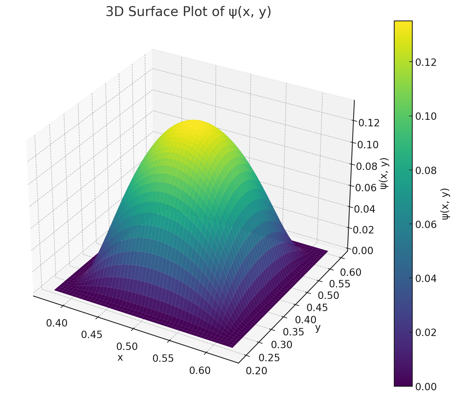
Figure 1: Bump function given by (4.10)

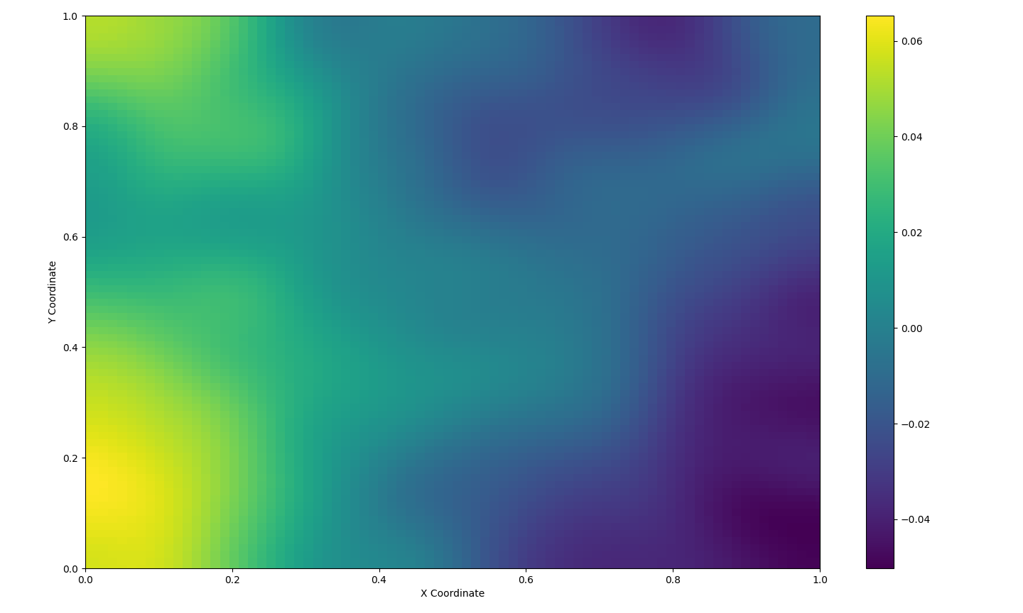
(a) Posterior mean, $S=1000$

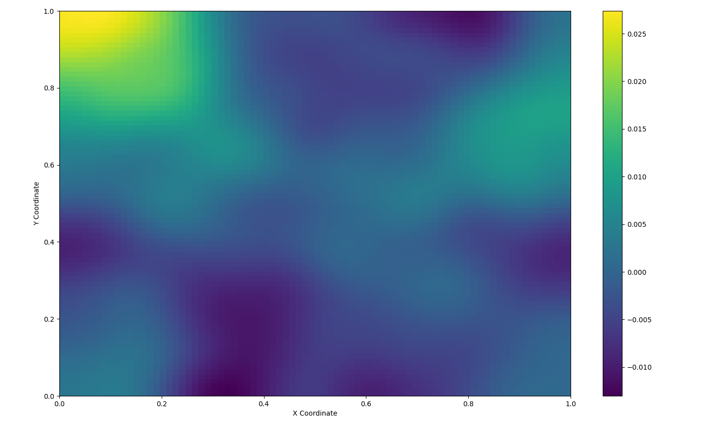
(b) Posterior mean, $S=5000$

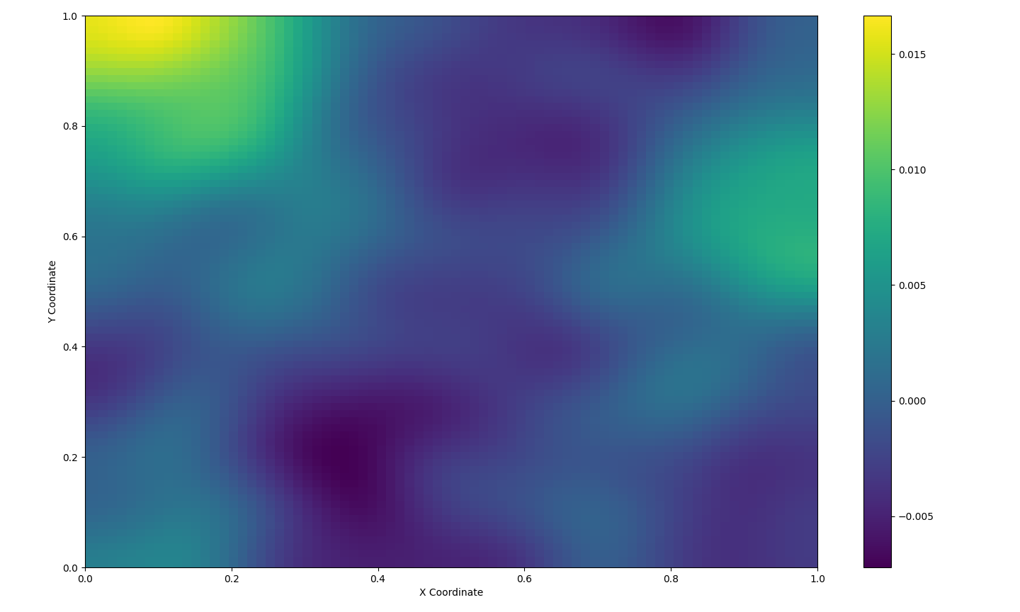
(c) Posterior mean, $S=10000$

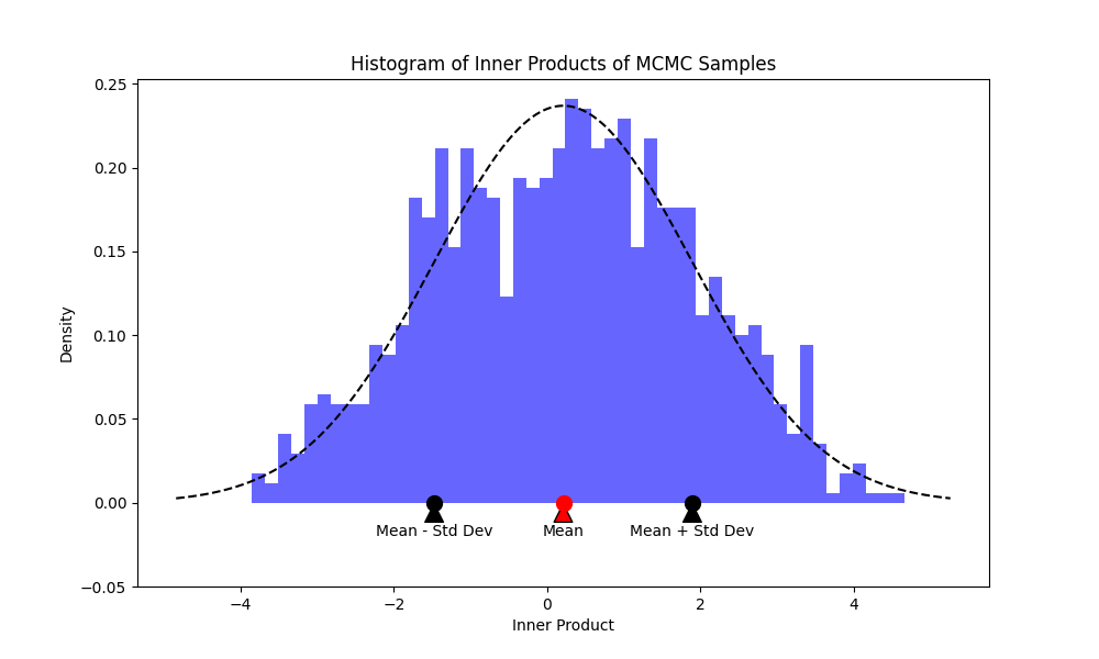
(d) Histogram of posterior draws for $\langle\psi,\theta\rangle$, $S=1000$

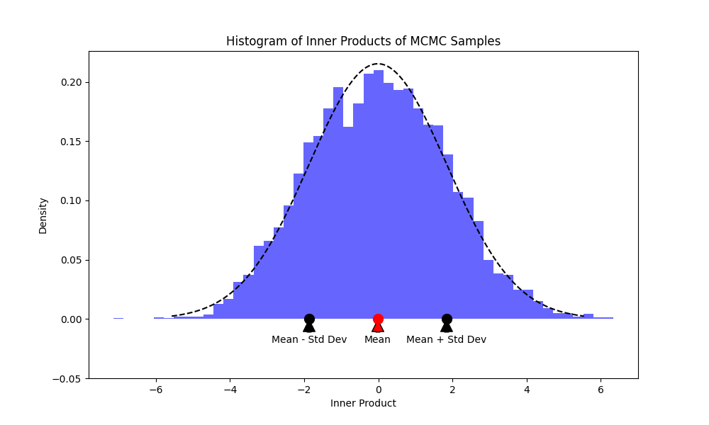
(e) Histogram of posterior draws for $\langle\psi,\theta\rangle$, $S=5000$

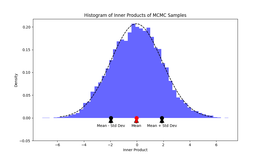
(f) Histogram of posterior draws for $\langle\psi,\theta\rangle$, $S=10000$

Figure 2: Posterior means and histograms of $\langle\psi,\theta\rangle$. Red dot: true value, green dot: mean, black dots: $\hat{m}\pm\hat{\sigma}$.

We illustrate our theory by numerical experiments for a two-dimensional Darcy flow equation. Using the notation of the previous section we assume

$$-\nabla(\alpha(\theta)\nabla u(x,y))=f(x,y)$$ (4.9)

Let $\theta_{0}\equiv 0$ and $a_{0}=e^{\theta_{0}}=1$. The resulting PDE with zero boundary data is an inhomogeneous Poisson equation

$$\begin{cases}-\Delta u(x,y)=f(x,y),\;&(x,y)\in(0,1)\times(0,1);\\ u(x,y)=0,\;&(x,y)\in[0,1]\times[0,1]\setminus(0,1)\times(0,1).\end{cases}$$

We choose $f=-2x(1-x)-2y(1-y)$. It is then to check that the unique solution is $u(x,y)=-xy(1-x)(1-y)$. We Consider now the following bump function

$$\psi(x,y)=\begin{cases}\exp\left\{-\left(\frac{1}{(8x-3)(5-8x)}+\frac{1}{(5y-1)(3-5y)}\right)\right\},\;&(x,y)\in\left(\frac{3}{8},\frac{5}{8}\right)\times\left(\frac{1}{5},\frac{3}{5}\right);\\ 0&\text{otherwise}.\end{cases}$$ (4.10)

While $\psi\in C_{0}^{\infty}(\mathcal{Z})$, it does not belong to $R(\mathbb{I}_{\theta_{0}}^{*})$, according to the integral curve argument similar to the one found in Nickl and Paternain (2022). Therefore, BvM cannot hold. However, since the conditions of our Theorem 3.1 is met for a Gaussian prior $\mathrm{Normal}(0,(-\Delta)^{\alpha})$, the coverage of Bayes credible set for $\langle\psi,\theta\rangle$ should be conservative. We apply this functional to our main theorems. We compute the observations for a 2 dimensional Darcy flow, which then corrupted by additive noise with $\sigma=5.0$.

We compute the posterior mean with MCMC method for functions as described in Cotter et al. (2013). The preconditioned Crank-Nicolson (pCN) algorithm is then used to compute $S=1000,5000,10000$ iterations of a Markov Chain targeting the posterior distribution of $\theta_{N}|D_{N}$, with $\beta=0.4$ In Figure 2, we display the histograms of the tracked quantities $\langle\theta_{s},\psi\rangle$. We use as linear functional the bump function given by (4.10). As observed in Figure 2 as $N$ increases the inner products approximate the normal distribution and the credible sets are centered around the true solution of the Darcy equations which is zero.

5 Proofs for section 3

5.1 Proof of Theorem 3.1

For this proof, we follow the proof of Theorem 3.7 in Monard, Nickl and Paternain (2021). We make some important modifications to account for the fact that $\psi$ need not belong to $R(\mathbb{I}_{\theta_{0}}^{*})$. The main idea is to show that the sequence of random variables (3.5) has a Laplace transform converging pointwise to the Laplace transform of a standard normal distribution. First, we write $\Pi_{N}^{\Theta_{\infty}(M,\overline{\epsilon}_{N})}(\cdot\mid\mathcal{D}^{N})$, the posterior distribution truncated and renormalized to the set $\Theta_{\infty}(M,\overline{\epsilon}_{N})$. For any Borel set $A\subset\Theta$, we have

$$\Pi_{N}(A\mid\mathcal{D}^{N})-\Pi^{\Theta_{\infty}(M,\overline{\epsilon}_{N})}(A\mid\mathcal{D}^{N})$$

$$=\Pi_{N}(\Theta_{\infty}(M,\overline{\epsilon}_{N})^{c}\cap A\mid\mathcal{D}^{N})-\Pi_{N}(\Theta_{\infty}(M,\overline{\epsilon}_{N})^{c}\mid\mathcal{D}^{N})\Pi_{N}^{\Theta_{\infty}(M,\overline{\epsilon}_{N})}(A\mid\mathcal{D}^{N}),$$

so the total variation distance between the posterior measure and its restriction to $\Theta_{\infty}(M,\overline{\epsilon}_{N})$ is bounded above as

$$\sup_{A\text{ Borel }}|\Pi_{N}(A\mid\mathcal{D}^{N})-\Pi_{N}^{\Theta_{\infty}(M,\overline{\epsilon}_{N})}(A\mid\mathcal{D}^{N})|\leq 2\Pi_{N}(\Theta_{\infty}(M,\overline{\epsilon}_{N})^{c}\mid\mathcal{D}^{N}).$$

By Assumption 7, the right hand side of the above equation is $o_{P_{\theta_{0}}}^{N}(1)$. Since the total variation topology is finer than the weak topology on measures, we also have

$$d_{\mbox{\tiny weak}}(\Pi_{N}(\cdot\mid\mathcal{D}^{N}),\Pi_{N}^{\Theta_{\infty}(M,\overline{\epsilon}_{N})}(\cdot\mid\mathcal{D}^{N}))=o_{P_{\theta_{0}}}^{N}(1).$$

Under these assumptions, it suffices to show the assertion of Theorem 3.1 holds for $\Pi_{N}^{\Theta_{\infty}(M,\overline{\epsilon}_{N})}(A\mid\mathcal{D}^{N})$.

We now show that the Laplace transform corresponding to the probability law of random variable $s_{N}^{-1}Z_{N}$ ((3.5)), induced by the truncated posterior measure $\Pi_{N}^{\Theta_{\infty}(M,\overline{\epsilon}_{N})}(\cdot\mid\mathcal{D}^{N})$:

$$\frac{\int_{\Theta_{\infty}(M,\overline{\epsilon}_{N})}e^{ts_{N}^{-1}Z_{N}-l_{N}(\theta)}~{}d\Pi_{N}(\theta)}{\int_{\Theta_{\infty}(M,\overline{\epsilon}_{N})}e^{-l_{N}(\theta)}~{}d\Pi_{N}(\theta)},$$ (5.1)

converges for each $t\in\mathbb{R}$ to $e^{t^{2}/2}$ in probability. If this claim is true, the convergence of the Theorem follows by Lemmas 1-2 of the Supplement (Castillo and Rousseau, 2015).

We now consider the following expansion of the numerator of (5.1),

$$\int_{\Theta_{\infty}(M,\overline{\epsilon}_{N})}e^{ts_{N}^{-1}Z_{N}-l_{N}(\theta)+l_{N}(\theta^{(t)})-l_{N}(\theta^{(t)})}~{}d\Pi_{N}(\theta),$$ (5.2)

where $\theta^{(t)}:=\theta-ts_{N}^{-1}\overline{\psi}_{N}$ for $\overline{\psi}_{N}$ defined in (3.8). Then:

$$l_{N}(\theta)-l_{N}(\theta^{(t)}) =\sum_{i=1}^{N}\frac{1}{2}(|Y_{i}-G(\theta)(X_{i})|^{2}-|Y_{i}-G(\theta^{(t)})(X_{i})|^{2})$$

$$=\sum_{i=1}^{N}\frac{1}{2}(|G(\theta)(X_{i})-G(\theta_{0})(X_{i})-\epsilon_{i}|^{2}-|G(\theta^{(t)})(X_{i})-G(\theta_{0})(X_{i})-\epsilon_{i}|^{2})$$

$$=\sum_{i=1}^{N}\underbrace{\left(\frac{|G(\theta)-G(\theta_{0})|^{2}(X_{i})}{2}-\frac{|G(\theta^{(t)})-G(\theta_{0})|^{2}(X_{i})}{2}\right)}_{(I)}$$

$$\quad-\underbrace{\sum_{i=1}^{N}\epsilon_{i}(G(\theta)-G(\theta_{0}))(X_{i})}_{(II)}.$$

We first expand the term (II) as

$$ts_{N}^{-1}\sum_{i=1}^{N}\epsilon_{i}\mathbb{I}_{\theta_{0}}(\overline{\psi}_{N})(X_{i})+\sum_{i=1}^{N}\epsilon_{i}R_{\theta_{0}}(\theta-\theta_{0}-ts_{N}^{-1}\overline{\psi}_{N})(X_{i})$$ (5.3)

By Lemma 1, the absolute supremum of the second summand in the above display over $\theta\in\Theta_{\infty}(M,\overline{\epsilon}_{N})$ is $o_{P_{\theta_{0}}}^{N}(1)$. Next, we expand the term (I) as

$$\sum_{i=1}^{N}\left(\frac{|G(\theta)-G(\theta_{0})|^{2}(X_{i})}{2}-\frac{\|G(\theta)-G(\theta_{0})\|_{L^{2}(\mathcal{X})}}{2}\right)$$ (5.4)

$$\quad+\sum_{i=1}^{N}\left(\frac{|G(\theta^{(t)})-G(\theta_{0})|^{2}(X_{i})}{2}-\frac{\|G(\theta^{(t)})-G(\theta_{0})\|_{L^{2}(\mathcal{X})}}{2}\right)$$ (5.5)

$$\quad-t^{2}s_{N}^{-1}\frac{N\|\mathbb{I}_{\theta_{0}}(\overline{\psi}_{N})\|^{2}_{L^{2}(\mathcal{X})}}{2}+ts_{N}^{-1}\langle\theta-\theta_{0},N\mathbb{I}_{\theta_{0}}^{*}\mathbb{I}_{\theta_{0}}(\overline{\psi}_{N})\rangle_{L^{2}(\mathcal{X})}$$ (5.6)

$$\quad+N\langle\mathbb{I}_{\theta_{0}}(\theta-\theta_{0}),R(\theta-\theta_{0})\rangle_{L^{2}(\mathcal{X})}-N\langle\mathbb{I}_{\theta_{0}}(\theta^{(t)}-\theta_{0}),R(\theta^{(t)}-\theta_{0})\rangle_{L^{2}(\mathcal{X})}$$ (5.7)

$$\quad+\frac{N\|R(\theta-\theta_{0})\|_{L^{2}(\mathcal{X})}^{2}}{2}-\frac{N\|R(\theta^{(t)}-\theta_{0})\|_{L^{2}(\mathcal{X})}^{2}}{2}$$ (5.8)

By Lemma 1, the absolute supremum of (5.4) and (5.5) over $\theta\in\Theta_{\infty}(M,\overline{\epsilon}_{N})$ is $o_{P_{\theta_{0}}}^{N}(1)$. The absolute value of (5.7) is bounded above by a $2N\sigma_{N}\overline{\epsilon}_{N}$ by the Cauchy-Schwarz inequality and thus is $o_{P_{\theta_{0}}}^{N}(1)$ by Assumption 8. Similarly, the absolute value of (5.8) is bounded above by $N\sigma_{N}^{2}$ which is $o_{P_{\theta_{0}}}^{N}(1)$. Putting the above together with (II) (5.3), we conclude that the numerator (5.2) of the Laplace transform can be re-written as

$$\exp\left(t^{2}s_{N}^{-2}\frac{\langle\overline{\psi}_{N},N\mathbb{I}_{\theta_{0}}^{*}\mathbb{I}_{\theta_{0}}(\overline{\psi}_{N})\rangle_{L^{2}(\mathcal{X})}}{2}\right)\times$$

$$\int_{\Theta_{\infty}(M,\overline{\epsilon}_{N})}e^{ts_{N}^{-1}\langle\theta-\theta_{0},\tau_{N}^{-2}\Lambda^{\alpha}(\overline{\psi}_{N})\rangle_{L^{2}(\mathcal{X})}-l(\theta^{(t)})}~{}d\Pi_{N}(\theta)\times e^{o_{P_{\theta_{0}}}^{N}(1)}.$$

Define a measure $\Pi_{N}^{\prime}$ as the pushforward measure under a shift map $T_{\overline{\psi}_{N}}:\theta\mapsto\theta+ts_{N}^{-1}\overline{\psi}_{N}$. Since $\overline{\psi}_{N}\in D(\Lambda^{\alpha})$ by construction, the Cameron-Martin theorem (2.4) implies

$$e^{ts_{N}^{-1}\langle\theta,\tau_{N}^{-2}\Lambda^{\alpha}(\overline{\psi}_{N})\rangle_{L^{2}(\mathcal{X})}}=\frac{d\Pi_{N}^{\prime}}{d\Pi_{N}}(\theta)\times\exp\left(t^{2}s_{N}^{-2}\frac{\|\tau_{N}^{-1}\Lambda^{\alpha/2}(\overline{\psi}_{N})\|_{L^{2}(\mathcal{X})}^{2}}{2}\right)$$

Therefore, the Laplace transform (5.1) can now be rewritten as

$$\exp\bigg{(}-ts_{N}^{-1}\langle\theta_{0},\Lambda^{\alpha}(\overline{\psi}_{N})\rangle_{L^{2}(\mathcal{X})}+\frac{t^{2}}{2}\bigg{)}\times\frac{\int_{\Theta_{\infty}(M,\overline{\epsilon}_{N})}e^{-l_{N}(\theta^{(t)})}~{}d\Pi_{N}^{\prime}(\theta)}{\int_{\Theta_{\infty}(M,\overline{\epsilon}_{N})}e^{-l_{N}(\theta)}~{}d\Pi_{N}(\theta)}\times e^{o_{P_{\theta_{0}}}^{N}(1)}.$$ (5.9)

We may define the “bias” comprising the exponent of the first multiplier as

$$b_{N}\equiv b_{N}(\psi,\theta_{0})=\langle\theta_{0},\Lambda^{\alpha}(N\tau_{N}^{2}\mathbb{I}_{\theta_{0}}^{*}\mathbb{I}_{\theta_{0}}+\Lambda^{\alpha})^{-1}(\psi)\rangle_{L^{2}(\mathcal{Z})}.$$ (5.10)

Lemma 5 implies that under the condition we propose (3.10), we have $b_{N}/s_{N}\to 0$. Finally, we now observe that the quotient comprising the second multiplier is equal to

$$\frac{\int_{\Theta_{\infty}(M,\overline{\epsilon}_{N})}e^{-l_{N}(\theta^{(t)})}~{}d\Pi_{N}^{\prime}(\theta)}{\int_{\Theta_{\infty}(M,\overline{\epsilon}_{N})}e^{-l_{N}(\theta)}~{}d\Pi_{N}(\theta)}=\frac{\int_{{\Theta_{\infty}(M,\overline{\epsilon}_{N})}^{(t)}}e^{-l_{N}(\theta)}~{}d\Pi_{N}(\theta)}{\int_{\Theta_{\infty}(M,\overline{\epsilon}_{N})}e^{-l_{N}(\theta)}~{}d\Pi_{N}(\theta)},$$ (5.11)

where ${\Theta_{\infty}(M,\overline{\epsilon}_{N})}^{(t)}:=\Theta_{\infty}(M,\overline{\epsilon}_{N})-ts_{N}^{-1}\overline{\psi}_{N}$. Equation (5.11) is shown to converge in probability to 1, again by Lemma 1. Putting all the preceding facts together, we conclude that the simplified expression (5.9) converges in probability to $e^{t^{2}/2}$ for each $t\in\mathbb{R}$; hence, the conclusion

$$\mathbb{E}^{\Theta_{\infty}(M,\overline{\epsilon}_{N})}[e^{ts_{N}^{-1}Z_{N}}|\mathcal{D}^{N}]\stackrel{{\scriptstyle P}}{{\to}}\exp\left(\frac{t^{2}}{2}\right),$$ (5.12)

where $\mathbb{E}^{\Theta_{\infty}(M,\overline{\epsilon}_{N})}[\cdot|\mathcal{D}^{N}]$ is a notation introduced for expectations taken with respect to the truncated posterior $\Pi_{N}^{\Theta_{\infty}(M,\overline{\epsilon}_{N})}$. The Laplace transform (5.1) therefore converges pointwise in probability to the Laplace transform of a standard normal distribution, which proves Theorem 3.1.

Lemma 1.

Define

$$\mathcal{F}_{1}(t) :=\sup_{\theta\in\Theta_{\infty}(M,\overline{\epsilon}_{N})}\left|\sum_{i=1}^{N}\epsilon_{i}R_{\theta_{0}}(\theta-\theta_{0}-ts_{N}^{-1}\overline{\psi}_{N})(X_{i})\right|;$$

$$\mathcal{F}_{2}(t) :=\sup_{\theta\in\Theta_{\infty}(M,\overline{\epsilon}_{N})}\left|\sum_{i=1}^{N}\left(\frac{|G(\theta)-G(\theta_{0})|^{2}(X_{i})}{2}-\frac{\|G(\theta)-G(\theta_{0})\|_{L^{2}(\mathcal{X})}^{2}}{2}\right)\right|.$$

Then $\mathcal{F}_{1}(t)=o_{P_{\theta_{0}}^{N}}(1)$, $\mathcal{F}_{2}(t)=o_{P_{\theta_{0}}^{N}}(1)$ and the quotient in (5.11) is $\exp\left({o_{P_{\theta_{0}}^{N}}(1)}\right)$ for each $t\in\mathbb{R}$.

Proof.

The proof of the first two assertions follows the proof of Lemmas 4.3-4 in Monard, Nickl and Paternain (2021). We therefore do not reproduce the full proof here, but highlight the differences in the estimates that are needed to apply the previous argument. The full proof is in the Appendix.

The main idea behind showing $\mathcal{F}_{1}(t)=o_{P_{\theta_{0}}^{N}}(1)$ and $\mathcal{F}_{2}(t)=o_{P_{\theta_{0}}^{N}}(1)$ according to the is to use Assumption 8 to verify the sufficient conditions of Theorem 3.5.4 inGiné and Nickl (2021). Inspecting the proof of Lemmas 4.3-4 in Monard, Nickl and Paternain (2021), we observe that all the arguments of this proof apply identically and uniformly in $\theta\in\Theta_{\infty}(M,\overline{\epsilon}_{N})$, provided we can show that

$$s_{N}^{-1}\|\overline{\psi}_{N}\|_{L^{\infty}(\mathcal{Z})}\ll\overline{\epsilon}_{N}.$$ (5.13)

The reasoning is as follows. First, if the above statement is true, then for every fixed $t\in\mathbb{R}$ and uniformly in $\theta\in\Theta_{\infty}(M,\overline{\epsilon}_{N})$, we have

$$\|\theta-\theta_{0}-ts_{N}^{-1}\overline{\psi}_{N}\|_{L^{\infty}(\mathcal{Z})}\leq\|\theta-\theta_{0}\|+ts_{N}^{-1}\|\overline{\psi}_{N}\|_{L^{\infty}(\mathcal{Z})}\lesssim\overline{\epsilon}_{N},$$

where the multiplicative constant is uniform in $\theta\in\Theta_{\infty}(M,\overline{\epsilon}_{N})$ since $M$ is a constant. By Assumption 5, this implies that uniformly in $\theta_{0}\in\Theta_{\infty}(M,\overline{\epsilon}_{N})$,

$$R_{\theta_{0}}(\theta-\theta_{0}-ts_{N}^{-1}\overline{\psi}_{N})\lesssim\overline{\epsilon}_{N}^{\eta}.$$

Therefore, our choice of the sequence $\sigma_{N}$ from Assumption 8 is an upper bound also for $R_{\theta_{0}}(\theta-\theta_{0}-ts_{N}^{-1}\overline{\psi}_{N})$. For the proof of Lemmas 4.3-4 in Monard, Nickl and Paternain (2021), one can verify that these two consequences, along with Assumption 8, guarantee that each argument in Lemmas 4.3-4 in Monard, Nickl and Paternain (2021) is also applicable to our case. The statement (5.13) is true, as can be seen by combining Lemma 6 and the assumed condition (3.9).

We also claim that (5.11) converges in probability to 1. We recall the definition of the events $\Theta_{\infty}(M,\overline{\epsilon}_{N})$, as in (3.3), and ${\Theta_{\infty}(M,\overline{\epsilon}_{N})}^{(t)}=\Theta_{\infty}(M,\overline{\epsilon}_{N})-ts_{N}^{-1}\overline{\psi}_{N}$. Combination of Lemma 6 and the assumed condition (3.9) implies that $ts_{N}^{-1}\|\overline{\psi}_{N}\|_{L^{\infty}(\mathcal{Z})}\ll\overline{\epsilon}_{N}$ and $t\|\overline{\epsilon}_{N}\|_{H^{s}}\ll\overline{\epsilon}_{N}\ll M$, by Assumption 1 and since $s$ can be arbitrarily chosen as long as it belongs to $(\frac{d}{2},\alpha-\frac{d}{2})$. The assertion is therefore true. ∎

5.2 Proof of Theorem 3.2

By Lemma 7, $s_{N}=O(1/\sqrt{N})$ and the limit of $Ns_{N}^{2}$ is the same as $\|\varphi\|_{L^{2}(\mathcal{X})}^{2}$ for $\mathbb{I}_{\theta_{0}}^{*}\varphi=\psi$. Therefore, in the proof of Theorem 3.1, we can replace all appearances of $s_{N}$ with $\frac{\|\varphi\|_{L^{2}(\mathcal{X})}}{\sqrt{N}}$. One can then check that the same argument of the proof of Theorem 3.1 is applicable, given that one can verify:

1. $b_{N}$ (5.10) satisfies $s_{N}^{-1}b_{N}=o(1)$;

2. the second summand in (5.3) and terms (5.4)-(5.5) are all also $o_{P_{\theta_{0}}}^{N}(1)$ uniformly in $\theta\in\Theta_{\infty}(M,\overline{\epsilon}_{N})$;

3. the quotient (5.11) converges to 1 in probability.

All the above facts can be proven as follows. First, by Lemma 7 and condition (3.11), $s_{N}^{-1}b_{N}$ converges to zero. Second, by Lemma 9, we have $s_{N}^{-1}\|\psi_{\lambda}\|_{L^{\infty}(\mathcal{Z})}$ and $s_{N}^{-1}\|\psi_{\lambda}\|_{\widetilde{H}^{s}}$ bounded above by a constant multiple of $1/\sqrt{N}$ for any $s\in(\frac{d}{2},\alpha-\frac{d}{2})$. By Assumptions 3 and 7, it holds that the sequence $\overline{\epsilon}_{N}\gg 1/\sqrt{N}$. Therefore, as stated in the proof of Lemma 1, the arguments used in the proof of Lemmas 4.3-4 of Monard, Nickl and Paternain (2021) are again applicable, and the second statement can be proven. Finally, the very same arguments for the proof of the second statement also shows the quotient (5.11) converges in probability to 1, as outlined in the proof of Lemma 1.

5.3 Proof of Theorem 3.3

For the proof of this Theorem for either of the sufficient conditions (Theorem 3.1 or 3.2), we first claim that

$$d_{\mbox{\tiny weak}}(\mathcal{L}({\widehat{s}_{{}_{N}}}^{-1}\Psi(\overline{\theta}_{N}-\theta_{0})),\;\mathrm{Normal}(0,t_{N}/s_{N}))\to 0,$$ (5.14)

where $t_{N}$ defines the “approximate standard deviation” of the centering term $\widehat{\Psi}_{N}$ (3.6):

$$t_{N}:=\sqrt{N}\|\mathbb{I}_{\theta_{0}}(\overline{\psi}_{N})\|_{L^{2}(\mathcal{X})}.$$ (5.15)

Application of the central limit theorem shows that $t_{N}^{-1}\widehat{\Psi}_{N}$ converges weakly to a standard normal distribution. We observe that $t_{N}/s_{N}$ either converges to a finite nonzero constant $\leq 1$ or to zero, since $t_{N}<s_{N}$ for all finite $N$ by Lemma 5. In the latter case, the convergence statement can be made as

$$d_{\mbox{\tiny weak}}(\mathcal{L}(\widehat{s}_{{}_{N}}^{-1}\Psi(\overline{\theta}_{N}-\theta_{0}),\;\delta_{\{0\}})=o(1),$$

where $\delta_{\{0\}}$ is a Dirac mass at zero. In either case, the limiting measure, which we write as $Q$, is a tight probability measure on $\mathbb{R}$ and places zero probability mass on the boundary of the interval $[-z_{1-\gamma/2},\;z_{\gamma/2}]$. Now, by the Portmanteau theorem (Resnick, 2019), we deduce the convergence of the coverage probability:

$$P_{\theta_{0}}^{N}(\theta_{0}\in I_{N}) =P_{\theta_{0}}^{N}(\widehat{s}_{{}_{N}}^{-1}\Psi(\overline{\theta}_{N}-\theta_{0})\in[-z_{1-\gamma/2,\;z_{1-\gamma/2}}])$$

$$\to Q([-z_{1-\gamma/2},\;z_{1-\gamma/2}]).$$

The limiting probability belongs to the interval $(1-\gamma,1]$ whenever $t_{N}/s_{N}\to c\in[0,1)$ and is exactly $1-\gamma$ whenever $t_{N}/s_{N}\to 1$. By Lemma 8, the latter case holds if and only if $\psi\in R(\mathbb{I}_{\theta_{0}}^{*})$, which proves the assertion of the Theorem for both cases.

The proof of the claim (5.14) follows the proof of Theorem 3.8 in Monard, Nickl and Paternain (2021). We do not reproduce the full proof here, but highlight the differences in the estimates that are needed to apply the previous argument. Readers interested in the full proof can refer to the Appendix.

We first claim that all $p$-th moments of $s_{N}^{-1}Z_{N}$ are stochastically bounded thus:

$$s_{N}^{-2p}\mathbb{E}[Z_{N}^{2p}\mid\mathcal{D}^{N}]=O_{P_{\theta_{0}}^{N}}(1).$$ (5.16)

We can then recognize that the assertion of Lemma 4.6 (Monard, Nickl and Paternain, 2021) is a special case of (5.16) when $s_{N}\asymp 1/\sqrt{N}$ and $p=1$. Inspection of the proof of Lemma 4.6 shows that the same arguments are applicable for general $p$ and $s_{N}$ for the general power $p$, accommodating the order estimate of $s_{N}$ from Lemmas 5 and 7. The modifications are technical and do not change the essence of the previous authors’ method, so we relegate the details to the Appendix. Provided we can show that the assertion (5.16) is also true, the remaining proof of the claim (5.14) follows by a contradiction argument identical to the proof in section 4.5 of Monard, Nickl and Paternain (2021).

5.4 Asymptotics of Key Quantities

The proof of our main results relies on characterizing the asymptotics of three quantities: $s_{N}$ (3.7), $t_{N}$ (5.15) and $b_{N}$ (5.10), along with the $L^{\infty}(\mathcal{Z})$-norm of $\overline{\psi}_{N}$ (3.8). Note that all of these quantities do not depend on $\theta$, so that all inequalities in this section do not specify the exact multiplicative constants.

For the results that follow, we first define a new linear bounded operator from $L^{2}(\mathcal{Z})$ to $L^{2}(\mathcal{X})$

$$\mathbb{K}_{\theta_{0},\alpha}:=\mathbb{I}_{\theta_{0}}\Lambda^{-\alpha/2}.$$ (5.17)

We then observe that $\mathbb{K}_{\theta_{0},\alpha}^{*}\mathbb{K}_{\theta_{0},\alpha}$ is a positive, self-adjoint, injective (due to Assumption 6) linear operator on $L^{2}(\mathcal{X})$ and is trace-class, its trace being bounded above by the operator norm of $\mathbb{I}_{\theta_{0}}^{*}\mathbb{I}_{\theta_{0}}$ times the trace of $\Lambda^{-\alpha}$. It possesses an eigendecomposition consisting of positive eigenvalues and eigenvectors that form an orthonormal bases of $L^{2}(\mathcal{X})$.

Lemma 2.

Let $\psi\in L^{2}(\mathcal{Z})$. Under Assumption 6, there exists $b>0$ and $C=C(\psi,\Lambda,\alpha,\beta)>0$ such that

$$\langle\psi_{\lambda},\psi_{\lambda}-u\rangle_{L^{2}(\mathcal{Z})}\leq\frac{1-b}{2}\|\psi_{\lambda}-u\|_{L^{2}(\mathcal{Z})}^{2}+C\|\mathbb{K}_{\theta_{0},\alpha}(\psi_{\lambda}-u)\|_{L^{2}(\mathcal{X})}^{\eta^{\mathrm{lin}}},$$ (5.18)

where $\psi_{\lambda}:=\Lambda^{-\alpha/2}\psi$.

Proof.

Write $\psi_{\lambda}:=\Lambda^{-\alpha/2}(\psi)\in\widetilde{H}^{\alpha}$. Observe that $\psi_{\lambda}\notin R((\mathbb{K}_{\theta_{0},\alpha}^{*}\mathbb{K}_{\theta_{0},\alpha})^{1/2})$ since we assumed $\psi\notin R((\mathbb{I}_{\theta_{0}}^{*}\mathbb{I}_{\theta_{0}})^{1/2})$. We show the following variational inequality is true for some $b>0$ and every $u\in L^{2}(\mathcal{Z})$: Fix some $b<1$. Whenever

$$\|u\|_{L^{2}(\mathcal{Z})}\geq\frac{1+b}{1-b}\|\psi_{\lambda}\|_{L^{2}(\mathcal{Z})},$$

by the triangle and Cauchy-Schwarz inequality, the left hand side of the above equation is bounded above by

$$\|\psi_{\lambda}\|_{L^{2}(\mathcal{Z})}\|\psi_{\lambda}-u\|_{L^{2}(\mathcal{Z})}\leq\frac{1-b}{2}\|\psi_{\lambda}-u\|^{2}_{L^{2}(\mathcal{Z})}.$$

Whenever $u\in B_{L^{2}(\mathcal{Z})}(\frac{1+b}{1-b})$, again using the Cauchy-Schwarz inequality and the fact that $\psi_{\lambda}\in\widetilde{H}^{\alpha}$, we obtain an upper bound

$$\langle\psi_{\lambda},\psi_{\lambda}-u\rangle_{L^{2}(\mathcal{Z})}\leq\|\Lambda^{\alpha/2}\psi_{\lambda}\|_{L^{2}(\mathcal{Z})}\|\Lambda^{-\alpha/2}(\psi_{\lambda}-u)\|_{L^{2}(\mathcal{Z})}.$$

By Assumption 6, there exists a constant $C$, depending only on $\psi_{\lambda},\Lambda,\alpha$ and $\beta$, such that the right hand side of the above equation is bounded above by $C\|\mathbb{K}_{\theta_{0},\alpha}(\psi_{\lambda}-u)\|^{\eta^{\mathrm{lin}}}_{L^{2}(\mathcal{Z})}$. ∎

Next, for a fixed vector $u$, we introduce the distance function

$$d_{1/2}(R):=\inf_{v\in B_{L^{2}(\mathcal{X})}(R)}\|u-\mathbb{K}_{\theta_{0},\alpha}^{*}v\|.$$ (5.19)

It is clear from the definition that there exists a finite $R$ and a vector $v$ such that $d_{1/2}(R)=0$ whenever $u\in R(\mathbb{K}_{\theta_{0},\alpha}^{*})$.

The following result is proven by Hofmann (2006) (Lemma 2.5).

Lemma 3.

When $u\notin R(\mathbb{K}_{\theta_{0},\alpha}^{*})$, the function (5.19) is positive, continuous, strictly decreasing, and convex. Furthermore, for each $R$, there exists a unique vector $v^{\dagger}\in B_{L^{2}(\mathcal{Z})}(R)$ which is orthogonal to the nullspace of $\mathbb{K}_{\theta_{0},\alpha}^{*}$ and satisfies

$$d_{1/2}(R)=\|u-(\mathbb{K}_{\theta_{0},\alpha}^{*}\mathbb{K}_{\theta_{0},\alpha})^{1/2}v^{\dagger}\|_{L^{2}(\mathcal{Z})}.$$

Next, we derive the asymptotic order of the distance function for a vector $\psi_{\lambda}$ as $R\to\infty$, which plays an important role in our analysis.

Lemma 4.

Let $\psi\notin R(\mathbb{I}_{\theta_{0}}^{*})$ and let the corresponding distance function (5.19) be defined with respect to $u\equiv\psi_{\lambda}=\Lambda^{-\alpha/2}\psi$. Under Assumption 6, $d_{1/2}(R)\asymp R^{-\frac{\omega}{1-\omega}}$ as $R\to\infty$, with $\omega=\frac{\eta^{\mathrm{lin}}}{2-\eta^{\mathrm{lin}}}$.

Proof.

Since $\psi\notin R(\mathbb{I}_{\theta_{0}}^{*})$, $\psi_{\lambda}\notin R(\mathbb{K}_{\theta_{0},\alpha}^{*})$, due to the injectivity of $\Lambda^{-\alpha/2}$. The assertion now follows from combining Lemma 2 with Theorem 4.5 or Remark 4.6 of Flemming (2012). ∎

We are now ready to state the main lemmas needed for the proof of Theorem 3.1.

Lemma 5.

Let $\psi\notin R(\mathbb{I}_{\theta_{0}}^{*})$. Under Assumption 6, $s_{N}$ (3.7), $t_{N}$ (5.15) and $b_{N}$ (5.10) satisfy the following.

1. We have $t_{N}<s_{N}$ for every finite $N$ and

   $$s_{N}\asymp\tau_{N}\times(\sqrt{N}\tau_{N})^{-\omega},\;\omega=\frac{\eta^{\mathrm{lin}}}{2-\eta^{\mathrm{lin}}}.$$

2. We have

   $$s_{N}^{-1}b_{N}\lesssim\tau_{N}^{-1}\times\begin{cases}(\sqrt{N}\tau_{N})^{\omega(1-\frac{\beta}{\alpha})}\;&\text{ if }\alpha\geq\beta,\\ (\sqrt{N}\tau_{N})^{-\omega(1-\frac{\alpha}{\beta})}&\text{ if }\alpha<\beta.\end{cases}$$

   The exponents in the two cases above are non-negative and strictly negative, respectively.

Proof.

We use notions from spectral projection theory and functional calculus for self-adjoint operators; see section 2.3 of Engl, Hanke and Neubauer (1996). Define the spectral distribution function $F_{\psi_{\lambda}}(\epsilon)$ and the spectral projection operator $E_{t}$ through

$$F^{2}_{\psi_{\lambda}}(t):=\|E_{t}\psi_{\lambda}\|^{2}=\|\mathbf{1}_{(0,t]}(\mathbb{K}_{\theta_{0},\alpha}^{*}\mathbb{K}_{\theta_{0},\alpha})\psi_{\lambda}\|_{L^{2}(\mathcal{Z})}^{2},$$

where $\mathbf{1}_{(0,t]}$ is the indicator function on the interval $(0,t]$. We will first show that the spectral distance function yields the order of the lower and upper bound for $s_{N}$ and the upper bound for $t_{N}$, then use interpolation to deduce the second assertion about the bias term $b_{N}$.

1. By Lemma 4 and the equivalence relations of Theorem 2 (Flemming, Hofmann and Mathé, 2011), we obtain the fact

   $$F_{\psi_{\lambda}}(\epsilon)\asymp\epsilon^{\frac{\omega}{2}}\text{ as }\epsilon\to 0.$$ (5.20)

   The two quantities $s_{N}$ and $t_{N}$ can be rewritten as follows:

   $$s_{N} =\tau_{N}\|f(\mathbb{K}_{\theta_{0},\alpha}^{*}\mathbb{K}_{\theta_{0},\alpha})\psi_{\lambda}\|_{L^{2}(\mathcal{Z})},$$

   $$t_{N} =\tau_{N}\|g(\mathbb{K}_{\theta_{0},\alpha}^{*}\mathbb{K}_{\theta_{0},\alpha})\psi_{\lambda}\|_{L^{2}(\mathcal{Z})};$$

   where $f,g:(0,\infty)\to\mathbb{R}$ are defined as $f(x)=\frac{1}{\sqrt{1+N\tau_{N}^{2}x}}$ and $g(x)=\frac{\sqrt{N\tau_{N}^{2}x}}{(1+N\tau_{N}^{2}x)}$. This representation shows that $t_{N}<s_{N}$ for every finite $N$, proving the first part of the claim. We now observe that $f,f^{2},g$ are continuous and bounded above by 1. For $f$ and $f^{2}$, by strict monotonicity, there exists some $c>0$ such that whenever $x\in(0,\frac{c}{N\tau_{N}^{2}}]$, we have $f(x)\wedge f^{2}(x)\geq 1/2$. As a result we have

   $$s_{N}^{2}\geq\tau_{N}^{2}\int_{0}^{\frac{c}{N\tau_{N}^{2}}}f^{2}(t)~{}dF^{2}_{\psi_{\lambda}}(t)\geq\frac{\tau_{N}^{2}}{4}\int_{0}^{\frac{c}{N\tau_{N}^{2}}}~{}dF_{\psi_{\lambda}}(t)^{2}=\frac{\tau_{N}^{2}}{4}F^{2}\left(\frac{c}{N\tau_{N}^{2}}\right).$$ (5.21)

   By similar reasoning, we can also show

   $$h_{N}:=\|f^{2}(\mathbb{K}_{\theta_{0},\alpha}^{*}\mathbb{K}_{\theta_{0},\alpha})\psi_{\lambda}\|_{L^{2}(\mathcal{Z})}\geq\frac{1}{2}F\left(\frac{c}{N\tau_{N}^{2}}\right).$$ (5.22)

   This estimate will be needed for the proof later.

   To derive the upper bound, following the proof of Theorem 5.5 in Hofmann and Mathé (2007), we proceed as follows. First, consider the equation

   $$\Phi_{1/2}(R):=\frac{d_{1/2}(R)}{R}=\sqrt{\epsilon}.$$ (5.23)

   As shown by Hofmann and Mathé (2007) and Flemming, Hofmann and Mathé (2011), $\Phi_{\psi_{\lambda}}:(0,\infty)\to(0,\infty)$ is a continuous, strictly decreasing function for $\psi_{\lambda}\notin R(\mathbb{K}_{\theta_{0},\alpha}^{*})$. Therefore, the above equation has a unique solution $\widehat{R}=\widehat{R}(\epsilon)$ for all $\epsilon$. Now, observe that there exists some $c^{\prime}>0$ such that the mappings $x\mapsto\sqrt{x}f(x)$, $x\mapsto\sqrt{x}g(x)$, and $x\mapsto\sqrt{x}f^{2}(x)$ are all bounded above by $\frac{c^{\prime}}{\sqrt{N}\tau_{N}}$. Choose $\epsilon=\frac{1}{N\tau_{N}^{2}}$, $\widehat{R}=\widehat{R}(N)$ the solution of (5.23) for this choice, and $v^{\dagger}$ is the minimizer of the distance function (5.19) for this choice of $\widehat{R}$. Then, for $s_{N}$:

   $$\tau_{N}^{-1}s_{N} =\|f(\mathbb{K}_{\theta_{0},\alpha}^{*}\mathbb{K}_{\theta_{0},\alpha})\psi_{\lambda}\|_{L^{2}(\mathcal{Z})}$$

   $$\leq\|f(\mathbb{K}_{\theta_{0},\alpha}^{*}\mathbb{K}_{\theta_{0},\alpha})(\psi_{\lambda}-\mathbb{K}_{\theta_{0},\alpha}^{*}v^{\dagger})\|_{L^{2}(\mathcal{Z})}+\|f(\mathbb{K}_{\theta_{0},\alpha}^{*}\mathbb{K}_{\theta_{0},\alpha})\mathbb{K}_{\theta_{0},\alpha}^{*}v^{\dagger}\|_{L^{2}(\mathcal{Z})}$$

   $$\leq d_{1/2}(\widehat{R})+\frac{c^{\prime}}{\sqrt{N}\tau_{N}}\widehat{R}$$

   $$\leq(1+c^{\prime})d_{1/2}\left(\Phi_{1/2}^{-1}\left(\frac{1}{\sqrt{N}\tau_{N}}\right)\right).$$

   By Corollary 1 in Flemming, Hofmann and Mathé (2011), for every $\epsilon\in(0,\infty)$,

   $$d_{1/2}(2\Phi_{1/2}^{-1}(\sqrt{\epsilon}))\leq F_{\psi_{\lambda}}(\epsilon)\leq 2d_{1/2}(\Phi_{1/2}^{-1}(\sqrt{\epsilon})).$$

   Since $(2\epsilon)^{\frac{\omega}{1-\omega}}\leq 2^{\frac{\omega}{1-\omega}}\epsilon^{\frac{\omega}{1-\omega}}$, for $\epsilon$ belonging to a sufficiently small neighborhood of zero, the upper bound of the above equation can be bounded above by $2^{-\frac{\omega}{1-\omega}}$ times the lower bound due to Lemma 4. Combined with the lower bound (5.21) and the asymptotic estimate (5.20), this shows that $s_{N}\asymp\tau_{N}\times(N\tau_{N}^{2})^{-\omega/2}$. The same reasoning can be applied to an upper bound of $h_{N}$ from (5.22), so that $h_{N}\asymp(N\tau_{N}^{2})^{-\omega/2}$.

2. We now consider the estimate for $b_{N}$. For $\theta_{0}\in\widetilde{H}^{\beta}$, we may rewrite, using the Cauchy-Schwarz inequality,

   $$|b_{N}|\leq\|\theta_{0}\|_{\widetilde{H}^{\beta}}\times\|f^{2}(\mathbb{K}_{\theta_{0},\alpha}^{*}\mathbb{K}_{\theta_{0},\alpha})\psi_{\lambda}\|_{\widetilde{H}^{\alpha-\beta}}.$$ (5.24)

   When $\beta<\alpha$, using the interpolation inequality of Theorem 2.1,

   $$\|f^{2}(\mathbb{K}_{\theta_{0},\alpha}^{*}\mathbb{K}_{\theta_{0},\alpha})\psi_{\lambda}\|_{\widetilde{H}^{\alpha-\beta}}\leq\|f^{2}(\mathbb{K}_{\theta_{0},\alpha}^{*}\mathbb{K}_{\theta_{0},\alpha})\psi_{\lambda}\|_{L^{2}(\mathcal{Z})}^{\frac{\beta}{\alpha}}\|f^{2}(\mathbb{K}_{\theta_{0},\alpha}^{*}\mathbb{K}_{\theta_{0},\alpha})\psi_{\lambda}\|_{\widetilde{H}^{\alpha}}^{\frac{\alpha-\beta}{\alpha}}.$$ (5.25)

   Since $f^{2}(\mathbb{K}_{\theta_{0},\alpha}^{*}\mathbb{K}_{\theta_{0},\alpha})$ has an operator norm bounded by 1 for every $N$ and $\psi_{\lambda}=\Lambda^{-\alpha/2}\psi$, the $\widetilde{H}^{\alpha}$-norm of $f^{2}(\mathbb{K}_{\theta_{0},\alpha}^{*}\mathbb{K}_{\theta_{0},\alpha})\psi_{\lambda}$ is bounded above by the $L^{2}(\mathcal{Z})$-norm of $\psi$. The $L^{2}$-norm of the same vector is exactly $h_{N}$ in (5.22), which was shown above to be of order $(N\tau_{N}^{2})^{-\omega/2}$. Therefore, combined with the estimate for $s_{N}$, we conclude that

   $$s_{N}^{-1}b_{N}\lesssim\tau_{N}^{-1}\times(N\tau_{N}^{2})^{\frac{\omega}{2}(1-\frac{\beta}{\alpha})},$$

   which proves the second assertion of the Lemma for this case. In the second situation, where $\beta\geq\alpha$, we can again use interpolation and the fact that $\|\cdot\|_{\widetilde{H}^{-\beta}}\leq\|\cdot\|_{\widetilde{H}^{-\alpha}}$ to deduce

   $$\|f^{2}(\mathbb{K}_{\theta_{0},\alpha}^{*}\mathbb{K}_{\theta_{0},\alpha})\psi_{\lambda}\|_{\widetilde{H}^{\alpha-\beta}}\leq\|f^{2}(\mathbb{K}_{\theta_{0},\alpha}^{*}\mathbb{K}_{\theta_{0},\alpha})\psi_{\lambda}\|_{\widetilde{H}^{-\alpha}}^{\frac{\beta-\alpha}{\beta}}\|f^{2}(\mathbb{K}_{\theta_{0},\alpha}^{*}\mathbb{K}_{\theta_{0},\alpha})\psi_{\lambda}\|_{L^{2}(\mathcal{Z})}^{\frac{\alpha}{\beta}}.$$ (5.26)

   Since $\|f^{2}(\mathbb{K}_{\theta_{0},\alpha}^{*}\mathbb{K}_{\theta_{0},\alpha})\psi_{\lambda}\|_{\widetilde{H}^{-\alpha}}$ is equal to $\|\Lambda^{-\alpha/2}f^{2}(\mathbb{K}_{\theta_{0},\alpha}^{*}\mathbb{K}_{\theta_{0},\alpha})\psi_{\lambda}\|_{L^{2}(\mathcal{Z})}$, by Assumption 6, the $\widetilde{H}^{-\alpha}$-norm of $f^{2}(\mathbb{K}_{\theta_{0},\alpha}^{*}\mathbb{K}_{\theta_{0},\alpha})\psi_{\lambda}$ appearing in the right hand side is bounded above by a constant multiple of the factor

   $$\left(\frac{1}{\sqrt{N}\tau_{N}}\|g(\mathbb{K}_{\theta_{0},\alpha}^{*}\mathbb{K}_{\theta_{0},\alpha})\psi_{\lambda}\|_{L^{2}(\mathcal{Z})}\right)^{\eta^{\mathrm{lin}}\frac{\beta-\alpha}{\beta}}\asymp\left\{(N\tau_{N}^{2})^{-\frac{1}{2}-\frac{\omega}{2}}\right\}^{\eta^{\mathrm{lin}}\frac{\beta-\alpha}{\beta}}.$$

   Again using the estimates for $h_{N}$ and doing some algebra with the exponent, we obtain:

   $$s_{N}^{-1}b_{N}\lesssim\tau_{N}^{-1}\times(N\tau_{N}^{2})^{-\frac{\omega}{2}(1-\frac{\alpha}{\beta})},$$

   concluding the proof of the second assertion of the Lemma.

∎

Lemma 6.

If $\psi\notin R(\mathbb{I}_{\theta_{0}}^{*})$, under Assumption 6, we have $s_{N}^{-1}\|\overline{\psi}_{N}\|_{L^{\infty}(\mathcal{Z})}\leq s_{N}^{-1}\|\overline{\psi}_{N}\|_{\widetilde{H}^{\alpha^{\prime}}}\lesssim\tau_{N}\times(\sqrt{N}\tau_{N})^{-\omega(1-\frac{\alpha^{\prime}}{\alpha})}$ for any $\alpha^{\prime}\in(\frac{d}{2},\alpha)$.

Proof.

Let $f$ be defined as in the proof of Lemma 5. For any choice of $\alpha^{\prime}$ under the assumed condition, $\|\cdot\|_{\widetilde{H}^{\alpha^{\prime}}}$ dominates $\|\cdot\|_{L^{\infty}(\mathcal{Z})}$ due to Assumption 1. By interpolating as in Theorem 2.1, we can write:

$$\|\overline{\psi}_{N}\|_{L^{\infty}(\mathcal{Z})}\leq\|\overline{\psi}_{N}\|_{\widetilde{H}^{\alpha^{\prime}}}\leq\|\overline{\psi}_{N}\|_{L^{2}(\mathcal{Z})}^{\frac{\alpha-\alpha^{\prime}}{\alpha}}\|\overline{\psi}_{N}\|_{\widetilde{H}^{\alpha}}^{\frac{\alpha^{\prime}}{\alpha}}.$$ (5.27)

The $\widetilde{H}^{\alpha}$-norm and $L^{2}(\mathcal{Z})$-norm of $\overline{\psi}_{N}$ is equal to $\tau_{N}^{2}$ times the term $h_{N}$ appearing in (5.22) and $\tau_{N}^{2}$ times the $\widetilde{H}^{-\alpha}$-norm of the vector $f^{2}(\mathbb{K}_{\theta_{0},\alpha}^{*}\mathbb{K}_{\theta_{0},\alpha})\psi_{\lambda}$ appearing in the previous proof, respectively. Since $\alpha>\alpha^{\prime}$, using the same reasoning as in the previous proof, we obtain the claimed upper bound on the $L^{\infty}(\mathcal{Z})$-norm. ∎

When $\psi$ does belong to the range of $\mathbb{I}_{\theta_{0}}^{*}$ as in Theorem 3.2, we obtain quite different asymptotics.

Lemma 7.

If $\psi\in R(\mathbb{I}_{\theta_{0}}^{*})$, then $Ns_{N}^{2}\to\|(\mathbb{I}_{\theta_{0}}^{*}\mathbb{I}_{\theta_{0}})^{-1/2}\psi\|_{L^{2}(\mathcal{Z})}^{2}$ and

$$s_{N}^{-1}b_{N}\lesssim\begin{cases}N^{\frac{\alpha-2\beta}{2\alpha}}\tau_{N}^{-\frac{2\beta}{\alpha}}&\text{ if }\alpha\geq\beta,\\ \frac{1}{\sqrt{N}\tau_{N}^{2}}&\text{ if }\alpha<\beta.\end{cases}$$

Proof.

First, we observe that if $\psi\in R(\mathbb{I}_{\theta_{0}}^{*})=R((\mathbb{I}_{\theta_{0}}^{*}\mathbb{I}_{\theta_{0}})^{1/2})$, then $\psi_{\lambda}=\Lambda^{-\alpha/2}\psi\in R((\mathbb{K}_{\theta_{0},\alpha}^{*}\mathbb{K}_{\theta_{0},\alpha})^{1/2})$. For $s_{N}$ (3.7), we have

$$Ns_{N}^{2}=N\tau_{N}^{2}\int_{0}^{K}\frac{1}{1+N\tau_{N}^{2}t^{2}}~{}dF^{2}_{\psi_{\lambda}}(t)=\int_{0}^{K}\left(\frac{N\tau_{N}^{2}t^{2}}{1+N\tau_{N}^{2}t^{2}}\right)~{}\frac{dF^{2}_{\psi_{\lambda}}(t)}{t^{2}},$$

where $K$ stands in for the operator norm of $\mathbb{K}_{\theta_{0},\alpha}^{*}\mathbb{K}_{\theta_{0},\alpha}$. We apply the dominated convergence theorem to the spectral distribution function with $dF_{\psi_{\lambda}}^{2}$, $(1/t)^{2}$ as an integrable envelope, and conclude the above equation converges to $\|(\mathbb{K}_{\theta_{0},\alpha}^{*}\mathbb{K}_{\theta_{0},\alpha})^{-1/2}\psi_{\lambda}\|_{L^{2}(\mathcal{Z})}^{2}=\|(\mathbb{I}_{\theta_{0}}^{*}\mathbb{I}_{\theta_{0}})^{-1/2}\psi\|_{L^{2}(\mathcal{Z})}^{2}$ as $N\to\infty$.

For $b_{N}$, we return to the Cauchy-Schwarz inequality of (5.24) in the proof of Lemma 5, where it was shown it suffices to bound the term

$$\|f^{2}(\mathbb{K}_{\theta_{0},\alpha}^{*}\mathbb{K}_{\theta_{0},\alpha})\psi_{\lambda}\|_{\widetilde{H}^{\alpha-\beta}}$$

for $f(x)=\frac{1}{\sqrt{1+N\tau_{N}^{2}x}}$. When $\alpha\geq\beta$, again using the interpolation inequality (5.25), it suffices to bound the $L^{2}(\mathcal{Z})$-norm instead, since the $\widetilde{H}^{\alpha}$-norm is bounded above by the $L^{2}(\mathcal{Z})$-norm of $\psi$. Under the stated assumption, there exists some $w\in B_{L^{2}(\mathcal{Z})}(R),\;R>0$, such that

$$\|f^{2}(\mathbb{K}_{\theta_{0},\alpha}^{*}\mathbb{K}_{\theta_{0},\alpha})\psi_{\lambda}\|_{L^{2}(\mathcal{Z})}=\|f^{2}(\mathbb{K}_{\theta_{0},\alpha}^{*}\mathbb{K}_{\theta_{0},\alpha})\mathbb{K}_{\theta_{0},\alpha}^{*}w\|_{L^{2}(\mathcal{Z})}=:\|\tilde{f}(\mathbb{K}_{\theta_{0},\alpha}^{*}\mathbb{K}_{\theta_{0},\alpha})w\|_{L^{2}(\mathcal{Z})},$$

where $\tilde{f}(x)=\frac{\sqrt{x}}{1+N\tau_{N}^{2}x}$. There exists $c^{\prime}>0$ such that $\tilde{f}(x)\leq\frac{c^{\prime}}{N\tau_{N}^{2}}$, so the right hand side of the above display can be bounded from above by $\frac{c^{\prime}R}{N\tau_{N}^{2}}$. The bound on $s_{N}^{-1}b_{N}$ for $\alpha\geq\beta$ follows because $s_{N}\asymp N^{-1/2}$. The bound for the case when $\alpha<\beta\iff\alpha-\beta<0$ follows by bounding the $\widetilde{H}_{\alpha-\beta}$ norm by the $L^{2}(\mathcal{Z})$-norm. ∎

Lemma 8.

The quantity $s_{N}/t_{N}\to 1$ if and only if $\psi\in R(\mathbb{I}_{\theta_{0}}^{*})$.

Proof.

We first claim that $s_{N}/t_{N}\to 1$ if and only if, for every $c>0$,

$$\int_{0}^{\frac{c}{\sqrt{N}\tau_{N}}}\frac{1}{1+N\tau_{N}^{2}t^{2}}~{}dF^{2}_{\psi_{\lambda}}(t)\ll\tau_{N}^{-2}s_{N}^{2}.$$ (5.28)

Given the claim, the order of the left hand side can be deduced as follows. Since the function $f(t)=\frac{1}{1+N\tau_{N}^{2}t}$ on the range of integration is bounded below by $1/(1+c)$ and above by 1, we have

$$F_{\psi_{\lambda}}^{2}\left(\frac{1}{1+c}\frac{1}{N\tau_{N}^{2}}\right)\leq\int_{0}^{\frac{c}{\sqrt{N}\tau_{N}}}f(t)~{}dF^{2}_{\psi_{\lambda}}(t)\leq F^{2}_{\psi_{\lambda}}\left(\frac{1}{N\tau_{N}^{2}}\right).$$

If $\psi_{\lambda}\notin R(\mathbb{K}_{\theta_{0},\alpha}^{*})$, we also have $F_{\psi_{\lambda}}^{2}(\frac{1}{N\tau_{N}^{2}})\asymp\tau_{N}^{-2}s_{N}^{2}$, as shown in the proof of Lemma 5. On the other hand, if $\psi_{\lambda}\in R(\mathbb{K}_{\theta_{0},\alpha}^{*})$, then $F_{\psi_{\lambda}}^{2}(\frac{1}{N\tau_{N}^{2}})\ll\frac{1}{N\tau_{N}^{2}}$ by Lemma 3 (Flemming, Hofmann and Mathé, 2011), but $Ns_{N}^{2}$ converges to a finite nonzero limit by Lemma 7. Therefore, $s_{N}/t_{N}\to 1$ if and only if $\psi_{\lambda}\in R(\mathbb{K}_{\theta_{0},\alpha}^{*})$, which is if and only if $\psi\in R(\mathbb{I}_{\theta_{0}}^{*})$ by the injectivity of $\Lambda^{-\alpha/2}$.

The proof of the equivalence between the statement $s_{N}/t_{N}\to 1$ and (5.28) follows the argument used to prove Theorem 5.4 in Knapik, van der Vaart and van Zanten (2011). We reproduce their proof here for completeness. Write $s_{N}^{2}=A_{N}+B_{N}$ where

$$A_{N}:=\int_{\frac{c}{\sqrt{N}\tau_{N}}}^{K}f(t)~{}dF_{\psi_{\lambda}}^{2}(t),\;B_{N}:=\int_{0}^{\frac{c}{\sqrt{N}\tau_{N}}}f(t)~{}dF_{\psi_{\lambda}}^{2}(t),$$

where $K$ stands in for the operator norm of $\mathbb{K}_{\theta_{0},\alpha}^{*}\mathbb{K}_{\theta_{0},\alpha}$. Similarly, write $t_{N}^{2}=C_{N}+D_{N}$. Our goal is to show $t_{N}/s_{N}\to 1$ if and only if $B_{N}/A_{N}\to 0$.

We observe that $t_{N}$ can be written as

$$t_{N}=\int_{0}^{K}\frac{N\tau_{N}^{2}t^{2}}{1+N\tau_{N}^{2}t^{2}}\times f(t)~{}dF^{2}_{\psi_{\lambda}}(t),$$

so that

$$\frac{D_{N}}{B_{N}}\leq\frac{c}{1+c}\leq\frac{C_{N}}{A_{N}}\leq 1.$$

To show that $t_{N}/s_{N}\to 1$ implies $B_{N}/A_{N}\to 0$, we write

$$\frac{t_{N}^{2}}{s_{N}^{2}}=\frac{C_{N}/A_{N}+(D_{N}/B_{N})(B_{N}/A_{N})}{1+B_{N}/A_{N}}\leq\frac{1+(B_{N}/A_{N})c/(1+c)}{1+B_{N}/A_{N}}.$$

Fix $r\in(0,1)$. The mapping $x\mapsto\frac{1+rx}{1+x}$ is strictly decreasing from 1 (at $x=0$) to $r<1$ (as $x\to\infty$). It follows that the right hand side of the above equation converges to 1 if and only if $B_{N}/A_{N}\to 0$, with its limit infimum strictly smaller than 1 otherwise, which proves the implication $t_{N}/s_{N}\to 1\implies B_{N}/A_{N}\to 0$.

To show the other implication: $B_{N}/A_{N}\to 0\implies t_{N}/s_{N}\to 1$, we write

$$\frac{t_{N}^{2}}{s_{N}^{2}}\geq\frac{C_{N}}{A_{N}+B_{N}}=\frac{C_{N}/A_{N}}{1+B_{N}/A_{N}}\geq\frac{c/(1+c)}{1+B_{N}/A_{N}}.$$

If $B_{N}/A_{N}\to 0$, then the limit infimum of the left hand side is at least $c/(1+c)$. Since this is true for every $c>0$, we conclude that $t_{N}/s_{N}\to 1$. ∎

Lemma 9.

If $\psi\in R(\mathbb{I}_{\theta_{0}}^{*})$, then $s_{N}^{-1}\|\overline{\psi}_{N}\|_{L^{\infty}(\mathcal{Z})}\leq s_{N}^{-1}\|\overline{\psi}_{N}\|_{\widetilde{H}^{\alpha^{\prime}}}\lesssim N^{-1/2}$ for any $\alpha^{\prime}\in(\frac{d}{2},\alpha)$.

Proof.

The reasoning is very similar to the proof of Lemma 6: again, we use the interpolation in (5.27), and observe that it suffices to bound $\tau_{N}^{2}$ times the $L^{2}(\mathcal{Z})$-norm of the vector $f^{2}(\mathbb{K}_{\theta_{0},\alpha}^{*}\mathbb{K}_{\theta_{0},\alpha})\psi_{\lambda}$, or $h_{N}$ in (5.22). By using the result from the proof of Lemma 7, we obtain

$$s_{N}^{-1}\|\overline{\psi}_{N}\|_{\widetilde{H}^{\alpha^{\prime}}}\lesssim\tau_{N}^{2}\times\sqrt{N}\times\frac{1}{N\tau_{N}^{2}}=\frac{1}{\sqrt{N}}.$$

∎

[Acknowledgments] The authors would like to thank the anonymous referees, an Associate Editor and the Editor for their constructive comments that improved the quality of this paper. KP and SM were supported by the Max Planck Institute for Mathematics in the Sciences in Leipzig.

KP acknowledges the partial support of the project PNRR - M4C2 - Investimento 1.3, Partenariato Esteso PE00000013 - “FAIR - Future Artificial Intelligence Research” - Spoke 1 “Human-centered AI”, funded by the European Commission under the NextGeneration EU programme. SM would like to acknowledge partial funding from HFSP RGP005, NSF DMS 17-13012, NSF BCS 1552848, NSF DBI 1661386, NSF IIS 15-46331, NSF DMS 16-13261, as well as high-performance computing partially supported by grant 2016- IDG-1013 from the North Carolina Biotechnology Center as well as the Alexander von Humboldt Foundation, the BMBF and the Saxony State Ministry for Science.

Appendix A Full Proof of Lemma 1

All constants appearing line by line in this proof are understood to be uniform in $\theta\in\Theta_{\infty}(M,\overline{\epsilon}_{N})$, so we will omit the specific constants from the inequalities up to order in $N$.

$\mathcal{F}_{1}(t)$ in Lemma 1 is bounded from above by

$$\sup_{\theta\in\Theta_{\infty}(M,\overline{\epsilon}_{N})}\sum_{i=1}^{N}|\epsilon_{i}R_{\theta_{0}}(\theta-\theta_{0}-ts_{N}^{-1}\overline{\psi}_{N})(X_{i})|;$$

we bound the supremum of each individual stochastic summand over $\Theta_{\infty}(M,\overline{\epsilon}_{N})$ using Theorem 3.5.4 in Giné and Nickl (2021). There are no measurability issues in this regard, as discussed by the text or the comment at the end of the proof for Lemma 4.3 (Monard, Nickl and Paternain, 2021). We list several estimates needed for the application of this result. Define a corresponding empirical process as

$$f_{\theta}(Z):=\epsilon R_{\theta_{0}}(\theta-\theta_{0}-ts_{N}^{-1}\overline{\psi}_{N})(X),\;Z=(\epsilon,X)\in\mathbb{R}\times\mathcal{X}$$

and denote the “indexing set” for the empirical process as

$$\mathcal{F}=\{f_{\theta}(Z):\theta\in\Theta_{\infty}(M,\overline{\epsilon}_{N})\}.$$

First,

$$\sup_{\theta\in\Theta_{\infty}(M,\overline{\epsilon}_{N})}\mathbb{E}f_{\theta}^{2}(Z)\leq\sup_{\theta\in\Theta_{\infty}(M,\overline{\epsilon}_{N})}\|ts_{N}^{-1}\overline{\psi}_{N}\|_{L^{\infty}}^{2\rho}\lesssim\overline{\epsilon}_{N}^{2\rho}\leq\sigma_{N}^{2}.$$

Second,

$$\sup_{\theta\in\Theta_{\infty}(M,\overline{\epsilon}_{N})}\|R(\theta^{(t)}-\theta_{0})\|_{L^{\infty}}\lesssim\|\theta^{(t)}-\theta_{0}\|_{L^{\infty}}^{\eta}\lesssim\overline{\epsilon}_{N}^{\eta}(1+s_{N}^{-1}\|\overline{\psi}_{N}\|_{L^{\infty}})^{\eta}.$$

Combining Lemma 6 and the assumed condition (3.9), we deduce $s_{N}^{-1}\|\overline{\psi}_{N}\|_{L^{\infty}}\ll\overline{\epsilon}_{N}$, so the above equation is bounded from above. We can thus define a pointwise envelope function $F(Z)$ dominating $\sup_{\theta\in\Theta_{\infty}(M,\overline{\epsilon}_{N})}|f_{\theta}(Z)|$ that is almost surely positive and satisfies

$$\|F\|_{L^{2}(P)}\lesssim\overline{\epsilon}_{N}^{\eta},$$

and furthermore for any probability measure $Q$ on $\mathbb{R}\times\mathcal{X}$, belonging to a subset of discrete, finitely supported measures that is dense in the weak topology of measures, satisfies

$$\|F\|_{L^{2}(Q)}\lesssim\overline{\epsilon}_{N}^{\eta}s_{Q},\;$$

for $s_{Q}^{2}$ the variance of $Q$. Finally,

$$\|f_{\theta}-f_{\theta^{\prime}}\|_{L^{2}(Q)} \leq s_{Q}\|R(\theta^{(t)}-\theta_{0})-R({\theta^{\prime}}^{(t)}-\theta_{0})\|_{L^{\infty}}$$

$$\leq s_{Q}(\|G(\theta^{(t)})-G({\theta^{\prime}}^{(t)}\|_{L^{\infty}}+\|\mathbb{I}_{\theta_{0}}[\theta^{(t)}-{\theta^{\prime}}^{(t)}]\|_{L^{\infty}})$$

$$\lesssim\overline{\epsilon}_{N}^{-\eta}\|F\|_{L^{2}(Q)}\|\theta-\theta^{\prime}\|_{L^{\infty}}^{\eta}.$$

The above display implies that any $(\overline{\epsilon}_{N}\delta)^{1/\eta}$-covering of $\Theta_{\infty}(M,\overline{\epsilon}_{N})$ in $L^{\infty}$-norm induces a $\delta$-covering of $\mathcal{F}$. Using these estimates and some basic substitution in the integrals appearing therein, we apply Theorem 3.5.4 (Giné and Nickl, 2021) and derive an upper bound for the supremum of $f_{\theta}(Z)$ :

$$\mathbb{E}\sup_{\theta\in\Theta_{\infty}(M,\overline{\epsilon}_{N})}\left|\sum_{i=1}^{N}f_{\theta}(Z_{i})\right|\lesssim\sqrt{N}\max\left[\sqrt{N}J_{N}(\sigma_{N},1),\;\frac{\overline{\epsilon}_{N}^{\eta}\sqrt{\log N}}{\sigma_{N}^{2}}J_{N}(\sigma_{N},1)\right].$$

The upper bound consists of two terms appearing in Assumption 8 which are supposed to be $o(1)$. Hence, we conclude $\mathcal{F}_{1}(t)=o(1)$.

A very similar argument can be applied to $\mathcal{F}_{2}(t)$ in the display of Lemma 1. Re-define the notations $f_{\theta}(Z)$ and the corresponding collection $\mathcal{F}$ as

$$f_{\theta}(X):=|G(\theta)-G(\theta_{0})|^{2}(X),\;\mathcal{F}:=\{f_{\theta}(X):\theta\in\Theta_{\infty}(M,\overline{\epsilon}_{N})\},\;X\in\mathcal{X}.$$

The pointwise envelope $F$ for $f_{\theta}$ can be taken to be a constant multiple of $\overline{\epsilon}_{N}^{2\eta}$, since

$$\sup_{\theta\in\Theta_{\infty}(M,\overline{\epsilon}_{N})}\|G(\theta_{0})-G(\theta^{(t)})\|_{L^{\infty}}^{2}\lesssim\overline{\epsilon}_{N}^{2\eta}.$$

Since $\sup_{\theta\in\Theta_{\infty}(M,\overline{\epsilon}_{N})}\|G(\theta)\|_{L^{\infty}}$ is also bounded from above, we conclude

$$\|f_{\theta}-f_{\theta^{\prime}}\|_{L^{\infty}}\lesssim\|\theta-\theta^{\prime}\|_{L^{\infty}}^{\eta}$$

and a $(\overline{\epsilon}_{N}\delta)^{1/\eta}$-covering of $\Theta_{\infty}(M,\overline{\epsilon}_{N})$ in $L^{\infty}$-norm induces a $\delta$-covering of $\mathcal{F}$ in $L^{2}(Q)$-norm for any probability measure $Q$. Similar steps now show that

$$\mathbb{E}\sup_{\theta\in\Theta_{\infty}(M,\overline{\epsilon}_{N})}\left|\sum_{i=1}^{N}f_{\theta}(Z_{i})\right|\lesssim\sqrt{N}\overline{\epsilon}_{N}^{2\eta}J_{N}(1,\overline{\epsilon}_{N}^{2\eta}),$$

and Assumption 8 again guarantees the upper bound is $o(1)$.

Appendix B Remaining Proof of Theorem 3.3

All constants appearing line by line in this proof are understood to be uniform in $\theta\in\Theta_{\infty}(M,\overline{\epsilon}_{N})$, so we will omit the specific constants from the inequalities up to order in $N$.

The missing piece of the proof in the main text is the full proof of claim (5.16):

$$s_{N}^{-2p}\mathbb{E}[Z_{N}^{2p}|\mathcal{D}^{N}]=O_{P_{\theta_{0}}^{N}}(1),$$

which we reproduce here. The display above is bounded from above by

$$2^{2p-1}s_{N}^{-2p}\mathbb{E}[\Psi(\theta-\theta_{0})^{2p}|\mathcal{D}^{N}]+2^{2p-1}s_{N}^{-2p}(\widehat{\Psi}_{N}-\langle\theta_{0},\psi\rangle_{L^{2}(\mathcal{Z})})^{2p}.$$

The second term in the last decomposition is $O_{P_{\theta_{0}}}^{N}(1)$, as can be seen by the definition of $\widehat{\Psi}_{N}$ (3.6), for which we can apply the central limit theorem and the continuous mapping theorem. This shows the term is $O_{P_{\theta_{0}}^{N}}((t_{N}/s_{N})^{2p})$ which is at most $O_{P_{\theta_{0}}^{N}}(1)$ by Lemmas 5 and 8. Turning now to the first term in the decomposition : define $C_{N}:=\{\theta:\|\theta-\theta_{0}\|_{L^{\infty}}\leq M\overline{\epsilon}_{N}\}$, for $M$ some large constant to be chosen below. We write the first term in the decomposition further as a sum of two terms:

$$s_{N}^{-2p}\mathbb{E}[\Psi(\theta-\theta_{0})^{2p}\mathbf{1}_{C_{N}}|\mathcal{D}^{N}]+s_{N}^{-2p}\mathbb{E}[\Psi(\theta-\theta_{0})^{2p}\mathbf{1}_{C_{N}^{c}}|\mathcal{D}^{N}].$$

We first bound the second term. By Cauchy-Schwarz inequality, the term is bounded from above by

$$s_{N}^{-2p}\sqrt{E[\Psi(\theta-\theta_{0})^{4p}|\mathcal{D}^{N}]}\sqrt{\Pi[\theta:\|\theta-\theta_{0}\|_{L^{\infty}}>M\overline{\epsilon}_{N}|\mathcal{D}^{N}]}.$$

Using Assumption 7 and simply writing out the posterior measure, we obtain the in-probability inequality

$$P_{\theta_{0}}^{N}\left(E[\Psi(\theta-\theta_{0})^{4p}|\mathcal{D}^{N}]\Pi[\theta:\|\theta-\theta_{0}\|_{L^{\infty}}>M\overline{\epsilon}_{N}|\mathcal{D}^{N}]>s_{N}^{4p}\right)$$

$$\leq P_{\theta_{0}}^{N}\left(\frac{\int_{\Theta}\Psi(\theta-\theta_{0})^{4p}e^{-(l_{N}(\theta)-l_{N}(\theta_{0}))}~{}d\Pi_{N}(\theta)}{\int_{\Theta}e^{-(l_{N}(\theta)-l_{N}(\theta_{0}))}~{}d\Pi_{N}(\theta)}>s_{N}^{4p}e^{cN\epsilon_{N}^{2}}\right)+o(1).$$

We apply Lemma 1.3.3 (Monard, Nickl and Paternain, 2021), valid under our Assumptions 4, to bound from below the denominator appearing in the posterior probability and deduce, by Markov’s inequality:

$$P_{\theta_{0}}^{N}\left(E[\Psi(\theta-\theta_{0})^{4p}|\mathcal{D}^{N}]\Pi[\theta:\|\theta-\theta_{0}\|_{L^{\infty}}>M\overline{\epsilon}_{N}|\mathcal{D}^{N}]>s_{N}^{4p}\right)$$

$$\leq\|\psi\|_{L^{2}(\mathcal{Z})}^{4p}\times s_{N}^{-4p}e^{-cN\epsilon_{N}^{2}}\int_{\Theta}\|\theta-\theta_{0}\|_{L^{2}(\mathcal{Z})}^{4p}\int_{(\mathbb{R}\times\mathcal{X})^{N}}e^{-(l_{N}(\theta)-l_{N}(\theta_{0}))}~{}dP_{\theta_{0}}^{N}(\mathcal{D}^{N})~{}d\Pi_{N}(\theta)+o(1)$$

by setting $M$ large enough so that $c>A+3$ with $A$ from Assumption 3. Applying Fubini’s theorem to simplify the expression, we then observe that

$$\int_{\Theta}\|\theta-\theta_{0}\|_{L^{2}(\mathcal{Z})}^{4p}~{}d\Pi_{N}(\theta)=\tau_{N}^{4p}\int_{\Theta}\|\theta-\theta_{0}\|_{L^{2}(\mathcal{Z})}^{4p}~{}d\Pi(\theta).$$

Using Lemma 5 and the fact that $p\geq 1$, we conclude that

$$s_{N}^{-4p}\tau_{N}^{4p}e^{-cN\epsilon_{N}^{2}}\lesssim\tau_{N}^{4p}N^{2p}e^{-cN\epsilon_{N}^{2}}.$$

As mentioned in the main text, the above display is $o(1)$ due to the conditions on the sequences $\tau_{N}$ and $\epsilon_{N}$ stated by Assumptions 2 and 3. Hence, we conclude the entire probability is $o(1)$.

It remains to bound the term $s_{N}^{-2p}\mathbb{E}[\Psi(\theta-\theta_{0})^{2p}\mathbf{1}_{C_{N}}|\mathcal{D}^{N}]$. We further decompose it into

$$s_{N}^{-2p}\mathbb{E}^{\Theta_{\infty}(M,\overline{\epsilon}_{N})}[\Psi(\theta-\theta_{0})^{2p}\mathbf{1}_{A_{N}}|\mathcal{D}^{N}]+\{s_{N}^{-2p}\{\mathbb{E}[\Psi(\theta-\theta_{0})^{2p}\mathbf{1}_{A_{N}}]-\mathbb{E}^{\Theta_{\infty}(M,\overline{\epsilon}_{N})}[\Psi(\theta-\theta_{0})^{2p}\mathbf{1}_{A_{N}}]\}.$$

We recall that $\mathbb{E}^{\Theta}_{\infty}(M,\overline{\epsilon}_{N})[\cdot|\mathcal{D}^{N}]$ is a notation introduced in the proof of Theorem 3.3 as the expectation with respect to the posterior distribution of $\theta$, truncated to and renormalized over the event $\Theta_{\infty}(M,\overline{\epsilon}_{N})$. Since for $t^{2p}\leq 2^{p}e^{pt}$ for any nonnegative real $t$ and $s_{N}^{-1}\widehat{\Psi}_{N}=O_{P_{\theta_{0}}^{N}}(1)$, we can use the result (5.12) obtained at the end of the proof for Theorem 3.3 and deduce the upper bound

$$s_{N}^{-2p}\mathbb{E}^{\Theta_{\infty}(M,\overline{\epsilon}_{N})}[\Psi(\theta-\theta_{0})^{2p}\mathbf{1}_{A_{N}}|\mathcal{D}^{N}]\leq 2^{p}e^{s_{N}^{-2p}\widehat{\Psi}_{N}+\frac{1}{2}}\times e^{o_{P_{\theta_{0}}^{N}}(1)},$$

and hence the term is $O_{P_{\theta_{0}}^{N}}(1)$. Finally, by the definition of the event $C_{N}$ and denoting by $\|P,Q\|_{TV}$ the total variation distance between measures $P$ and $Q$, we deduce the inequalities

$$s_{N}^{-2p}\left|\int_{C_{N}}\Psi(\theta-\theta_{0})^{2p}[d\Pi_{N}(\theta|\mathcal{D}^{N})-d\Pi_{N}^{\Theta_{\infty}(M,\overline{\epsilon}_{N})}(\theta|\mathcal{D}^{N})]\right|$$

$$\leq M\left(\frac{\overline{\epsilon}_{N}}{s_{N}}\right)^{2p}\|\psi\|_{L^{1}(\mathcal{Z})}^{2p}\|\Pi_{N}(\cdot|\mathcal{D}^{N}),\Pi_{N}^{\Theta_{\infty}(M,\overline{\epsilon}_{N})}(\cdot|\mathcal{D}^{N})\|_{TV}$$

$$\lesssim\left(\frac{\overline{\epsilon}_{N}}{s_{N}}\right)^{2p}\Pi_{N}(\Theta_{\infty}(M,\overline{\epsilon}_{N})^{c}|\mathcal{D}^{N})$$

$$\lesssim\left(\frac{\overline{\epsilon}_{N}}{s_{N}}\right)^{2p}O_{P_{\theta_{0}}^{N}}(e^{-cN\epsilon_{N}^{2}}).$$

Combination of Assumptions 3 and 7, together with again Lemma 7, imposes the condition on the sequences $\tau_{N}$ and $\overline{\epsilon}_{N}$ that the factor $\overline{\epsilon}_{N}/s_{N}$ grows at most as some polynomial power of $N$, so the entirety of the above display is $o_{P_{\theta_{0}}^{N}}(1)$. This shows that the claim (5.16) is indeed true.

Appendix C Proofs for section 4

C.1 Proof of Theorem 4.1

The proof of the Theorem follows the proof of Theorems 4-5 in Giordano and Nickl (2020). We therefore will only highlight the major differences in choosing a different scaling rate $\tau_{N}$. Prior to the main proof, we will first establish a few quantitative estimates useful for all following proofs and also verify Assumptions 3-4, provided $\theta_{0}\in\widetilde{H}^{\beta},\;\beta>1+\frac{d}{2}$ (only the first assertion of Assumption 4 is needed for this Theorem).

Analytic Estimates

By the mean value theorem, for every $\theta,\theta_{0}\in B_{\widetilde{H}^{\beta^{\prime}}}(M)$, there exists some $\tilde{\theta}:\mathcal{Z}\to\mathbb{R}$ such that

$$a_{\theta}-a_{\theta_{0}}=e^{\theta}-e^{\theta_{0}}=e^{\tilde{\theta}}(\theta-\theta_{0}).$$

Recall that the Gaussian prior is supported on $\widetilde{H}^{s}$ whenever $s<\alpha-\frac{d}{2}$. If $\theta,\theta_{0}\in B_{\widetilde{H}^{s}}(M)$, then they are uniformly bounded in $\|\cdot\|_{C^{1}}$ by Assumption 1 and Hölder embedding of Sobolev spaces. A collection of elements $\tilde{\theta}$ for which the above inequality is met is also uniformly bounded in $\|\cdot\|_{C^{1}}$. This implies that

$$\|a_{\theta}-a_{\theta_{0}}\|_{C^{1}}\asymp\|\theta-\theta_{0}\|_{C^{1}},$$ (C.1)

where the multiplicative constant depends only on $M$. Furthermore, the above holds when the norm in $C^{1}$ is replaced with $L^{p}$ for any $p\in[1,\infty]$.

Equation 4.1 specifies a strongly elliptic divergence form operator $L_{a},\;a\in\mathcal{C}$. Recall that $\beta^{\prime}=s\wedge\beta>1+\frac{d}{2}$ by the assumption on the choice of $s$ and $\beta\geq s$. Whenever $a\in B_{H^{\beta^{\prime}}}(M)$, Proposition A.5.2 in Nickl (2023) yields an explicit expression for the constant $C\equiv C(\beta^{\prime},d,\mathcal{X},K_{\min},f,g,M)>0$ such that

$$\sup_{\|\theta\|_{\widetilde{H}^{\beta^{\prime}}}\leq M}\|G(\theta)\|_{H^{\beta^{\prime}+1}}\leq C<\infty.$$ (C.2)

The above equation also provides a uniform bound on $\|\cdot\|_{C^{\xi}}$ for any $\xi<\beta^{\prime}-\frac{d}{2}$ by Hölder embedding of Sobolev spaces.

Verifying the Assumptions

Assumption 3 is proven in Proposition 2.1.3 of Nickl (2023) for a constant $U$ that is uniform in $M$.

Assumption 4 : First, by Proposition 2.1.3 in Nickl (2023) for $\kappa_{1}=1$, there exists some $L(M)$ such that

$$\|G(\theta)-G(\theta_{0})\|_{L^{2}}\leq L(M)\|\theta-\theta_{0}\|_{(H^{1})^{*}}$$

whenever $\theta,\theta_{0}\in B_{\widetilde{H}^{s}}(M)$. where $(H^{1})^{*}$ is the topological dual space of $H^{1}$. Since $\widetilde{H}^{1}=H_{0}^{1}$, we have $\widetilde{H}^{-1}=H^{-1}=(H_{0}^{1})^{*}$. Since the norms ${\|\cdot\|}_{(H^{1})^{*}}$ and ${\|\cdot\|}_{H_{0}^{1}}$ are equivalent on $H_{0}^{1}$, we conclude the first inequality of Assumption 4 is also satisfied for $\kappa_{1}=1$.

We now show the second inequality is met for a certain exponent $\eta$ that depends on $d$. By Hölder embedding of $H^{1}$, we have

$$\|G(\theta)-G(\theta_{0})\|_{L^{\infty}}\leq\|G(\theta)-G(\theta_{0})\|_{H^{\xi}}$$

for any $\frac{d}{2}<\xi$. If $d=1$, then $\xi$ can be exactly 1. Furthermore, $G(\theta)=G(\theta_{0})$ on $\partial\mathcal{X}$, so by the Poincaré inequality the right hand side is equivalent to $\|\nabla G(\theta)-\nabla G(\theta_{0})\|_{L^{2}}$. By Lemma 1 (Richter, 1981),

$$\|\nabla G(\theta)-\nabla G(\theta_{0})\|_{L^{2}}\leq K_{\min}^{-1}\|\nabla G(\theta_{0})\|_{L^{2}}\|\theta-\theta_{0}\|_{L^{\infty}}.$$

We conclude that when $d=1$, the second claim of Assumption 4 is met with exponent $\eta=1$. Next, consider the case when $d>1$. Choosing $\xi>\frac{d}{2}$ and using the Sobolev interpolation inequality:

$$\|G(\theta)-G(\theta_{0})\|_{L^{\infty}}\leq\|G(\theta)-G(\theta_{0})\|_{H^{\xi}}\leq\|G(\theta)-G(\theta_{0})\|_{H^{1}}^{1-\frac{\xi-1}{\beta^{\prime}}}\|G(\theta)-G(\theta_{0})\|_{H^{\beta^{\prime}+1}}^{\frac{\xi-1}{\beta^{\prime}}}.$$

We conclude that when $d>1$, the claim is met with any exponent in $(0,\frac{\beta^{\prime}-d-1}{\beta^{\prime}})$.

Main Proof

Given the above Assumptions, we now prove the “pushforward posterior” of $G(\theta)$ contracts towards a neighborhood of $G(\theta_{0})$ :

$$P_{\theta_{0}}^{N}(\Pi_{N}(\theta:\|G(\theta)-G(\theta_{0})\|_{L^{2}}>M\epsilon_{N},\;\|\theta\|_{\widetilde{H}^{s}}>M|\mathcal{D}^{N})\geq e^{-LN\epsilon_{N}^{2}})\to 0.$$ (C.3)

Throughout this section, we write $d_{G}(\theta,\theta_{0}):=\|G(\theta)-G(\theta_{0})\|$. Given this claim, the results of Theorem 4.1 will be derived on a local stability estimate for the inverse of $G$. For the proof, it will suffice to show the following three statements hold for some sequence of measurable subsets $\Theta_{N}\subset\Theta$, for all sufficiently large $N$ and every nonnegative $A,B,C$:

$$\Pi_{N}(\theta:\|G(\theta)-G(\theta_{0})\|_{L^{2}}\leq M\epsilon_{N})\geq e^{-AN\epsilon_{N}^{2}};$$ (C.4)

$$\Pi_{N}(\Theta_{N}^{c})\leq e^{-BN\epsilon_{N}^{2}};$$ (C.5)

$$\log\mathcal{N}(\Theta_{N},d_{H},\epsilon_{N})\leq CN\epsilon_{N}^{2}.$$ (C.6)

Note, in particular, that the proof of condition (C.4) implies Assumption 3 for every choice of sequence $\epsilon_{N}$ maintained in this proof. Combination of Theorem 14 and Lemma 22 in Giordano and Nickl (2020) implies the claimed contraction theorem (C.3).

We choose the sequence of subsets $\Theta_{N}$ for a given prior $\Pi_{N}$ to be

$$\Theta_{N}:=\{B_{\widetilde{H}^{-1}}(M\epsilon_{N};\theta_{0})+B_{\widetilde{H}^{\alpha\wedge\beta}}(M\sqrt{N}\epsilon_{N}\tau_{N};\theta_{0})\}\cap B_{\widetilde{H}^{s}}(M).$$ (C.7)

We verify the conditions one by one. First, by Assumption 4, we have

$$\Pi_{N}(\theta:d_{G}(\theta,\theta_{0})\leq M\epsilon_{N})\geq\Pi_{N}\left(\theta:\|\theta-\theta_{0}\|_{\widetilde{H}^{-1}}\leq\frac{\epsilon_{N}}{L(M^{\prime})},\;\|\theta-\theta_{0}\|_{\widetilde{H}^{s}}\leq M\right)$$ (C.8)

with $M^{\prime}=M+\|\theta_{0}\|$, through the triangle inequality. The event in the above equation is a symmetric set shifted by a fixed vector $\theta_{0}\in\widetilde{H}^{\beta}$. If $\alpha\leq\beta$, $\theta_{0}$ belongs to the Cameron-Martin space $\widetilde{H}^{\alpha}$, so by Corollary 2.6.18 in Giné and Nickl (2021) and the Gaussian correlation inequality, we obtain a lower bound

$$e^{-\tau_{N}^{-2}\|\theta_{0}\|_{\widetilde{H}^{\alpha}}}\Pi_{N}\left(\theta:\|\theta\|_{(H^{1})^{*}}\leq\frac{\epsilon_{N}}{L(M^{\prime})}\right)\Pi_{N}(\theta:\|\theta\|_{\widetilde{H}^{s}}\leq M).$$

The two prior probabilities involved in the above display can then be bounded from below as in the proof of Lemma 16 in Giordano and Nickl (2020) by a term $e^{-AN\epsilon_{N}^{2}}$ in this case, for some $A>0$. By the choice of $\tau_{N}=\frac{1}{\sqrt{N}\epsilon_{N}}$ in the $\alpha\leq\beta$ case, condition (C.4) follows. On the other hand, suppose $\alpha>\beta$. Define a finite-dimensional projection of $\theta_{0}$ by

$$\theta_{0}^{(N)}:=E_{D}\theta_{0},$$

where $D=N^{\frac{d}{2\beta+2+d}}$ and $E_{D}=\mathbf{1}_{(0,D]}(-\Delta^{\alpha/2})$ is the spectral projection operator. By the well-known Weyl asymptotics for the Laplacian (Weyl, 1911) and the choice of $\epsilon_{N}$ for this case, we obtain

$$\|\theta_{0}^{(N)}-\theta_{0}\|_{\widetilde{H}^{-1}}\lesssim(D)^{-\frac{2}{d}\frac{\beta+1}{2\beta+2+d}}\|\theta_{0}\|_{\widetilde{H}^{\beta}}\lesssim\epsilon_{N}^{2}.$$

Similar reasoning also yields the estimates

$$\|\theta_{0}^{(N)}-\theta_{0}\|_{\widetilde{H}^{s}}\asymp\|\theta_{0}^{(N)}-\theta_{0}\|_{\widetilde{H}^{s}}\lesssim N^{-\frac{\beta-s}{2\beta+2+d}}\|\theta_{0}\|_{\widetilde{H}^{\beta}}\lesssim 1$$

and

$$\|\theta_{0}^{(N)}\|_{\widetilde{H}^{\alpha}}\lesssim N^{\frac{\alpha-\beta}{2\beta+2+d}}.$$

By the triangle inequality and by the fact that the $\widetilde{H}^{s}$-norm dominates the $\widetilde{H}^{-1}$-norm,

$$\Pi_{N}\left(B_{(H^{\kappa})^{*}}\left(\frac{\epsilon_{N}}{L(M^{\prime})};\theta_{0}\right)\cap B_{\widetilde{H}^{s}}(M;\theta_{0})\right)\geq\Pi_{N}\left(B_{(H^{\kappa})^{*}}\left(\frac{\epsilon_{N}}{2L(M^{\prime})};\theta_{0}^{(N)}\right)\cap B_{\widetilde{H}^{s}}(M;\theta_{0}^{(N)})\right),$$

and since $\theta_{0}^{(N)}\in\widetilde{H}^{\alpha}$, we again apply Corollary 2.6.18 in Giné and Nickl (2021) to obtain a lower bound

$$e^{-\tau_{N}^{-2}\|\theta_{0}^{(N)}\|_{\widetilde{H}^{\alpha}}}\Pi_{N}\left(\theta:\|\theta\|_{(H^{1})^{*}}\leq\frac{\epsilon_{N}}{2L(M^{\prime})}\right)\Pi_{N}(\theta:\|\theta\|_{\widetilde{H}^{s}}\leq M).$$

The choice of $\tau_{N}$ in the $\alpha>\beta$ case implies the first multiplier is bounded below by $e^{-AN\epsilon_{N}^{2}}$ in this case. The two other probabilities can be bounded from below using the same arguments as in the $\alpha\leq\beta$ case, but with a different choice of $\tau_{N}$ and $\epsilon_{N}$. Proceeding again as in the proof of Lemma 16 from Giordano and Nickl (2020), condition (C.4) follows.

The other two conditions (C.5) and (C.6) follow the proof of Lemmas 17 and 18 in Giordano and Nickl (2020), only with a different choice of sequences $\tau_{N}$ and $\epsilon_{N}$.

Conditional Stability Estimates

We now derive Theorem 4.1 from (C.3) based on conditional stability estimates as first proposed in Vollmer (2013). We retrace the steps taken by Giordano and Nickl (2020). First, under Assumption 9 and whenever $\theta=\theta_{0}$ on $\partial\mathcal{X}$, Proposition 2.1.7 in Nickl (2023) shows the existence of a constant $C=C(M,K_{\min},k_{1},k_{2},\mathcal{X},d,f,g)$ such that

$$\|a_{\theta}-a_{\theta_{0}}\|_{L^{2}}\leq C\|a_{\theta_{0}}\|_{C^{1}}\|G(\theta)-G(\theta_{0})\|_{H^{2}};$$

note that $\|\cdot\|_{C^{1}}$ of $a_{\theta_{0}}$ is bounded above by a constant multiple of $\|\theta_{0}\|_{\widetilde{H}^{\beta}}$. Interpolating between Sobolev scales and using the uniform bound (C.2), we can deduce

$$\|a_{\theta}-a_{\theta_{0}}\|_{L^{2}(\mathcal{Z})}\lesssim\|G(\theta)-G(\theta_{0})\|^{\frac{\beta^{\prime}-1}{\beta^{\prime}+1}}_{L^{2}}$$

where the multiplicative constant is uniform in $\theta\in B_{\widetilde{H}^{s}}(M)$. Using (C.1), the left hand side is bounded from below as a constant multiple of $\|\theta-\theta_{0}\|_{L^{2}}$. On the other hand, Corollary 1 in Richter (1981) shows that whenever $\theta=\theta_{0}$ on $\partial\mathcal{X}$,

$$\|a_{\theta}-a_{\theta_{0}}\|_{L^{\infty}(\mathcal{Z})}\leq C(k_{1},k_{2},u_{\theta_{0}})\|a_{\theta_{0}}\|_{C^{1}(\mathcal{Z})}\|G(\theta)-G(\theta_{0})\|_{C^{2}(\mathcal{X})}.$$

By Hölder embedding of $H^{\xi},\;\xi>2+\frac{d}{2}$ and again by interpolating between Sobolev scales, we can deduce

$$\|a_{\theta}-a_{\theta_{0}}\|_{L^{\infty}(\mathcal{Z})}\lesssim\|G(\theta)-G(\theta_{0})\|_{L^{\infty}(\mathcal{Z})}^{\frac{\beta^{\prime}-1-d/2}{\beta^{\prime}+1}}$$

up to a multiplicative constant uniform in $\theta\in B_{\widetilde{H}^{s}}(M)$, completing the proof.

C.2 Proof of Theorem 4.2

Case 1 : Range Condition Does Not Hold

We apply Theorem 3.3 in the case when $\psi\notin R(\mathbb{I}_{\theta_{0}}^{*})$. To do so, we verify the remaining Assumptions 5-8.

Assumption 5 is verified by Theorem 3.3.2 in Nickl (2023). In particular, we obtain an explicit expression for $\mathbb{I}_{\theta_{0}}$, its adjoint and the order of the remainder term (3.2):

$$\mathbb{I}_{\theta_{0}}(h)=-L_{a_{0}}^{-1}[\nabla\cdot(e^{\theta_{0}}h\nabla u_{a_{0}})],\; h\in L^{2}(\mathcal{Z});$$ (C.9)

$$\mathbb{I}_{\theta_{0}}^{*}(g)=e^{\theta_{0}}\nabla u_{a_{0}}\cdot\nabla L_{a_{0}}^{-1}[g],\; g\in L^{2};$$ (C.10)

$$\|R_{\theta_{0}}(h)\|_{L^{2}}=O(\|h\|_{L^{\infty}(\mathcal{Z})}^{2}),\; h\in L^{2}(\mathcal{Z}).$$ (C.11)

Assumption 6 : Since $\alpha>1+d$, every $h\in\widetilde{H}^{\alpha}$ also belongs to $\widetilde{H}^{1}=H_{0}^{1}$, the domain of $(-\Delta)^{1/2}$. For every such $h$, by Theorem 5 in Nickl and Paternain (2022), we have

$$C\|\mathbb{I}_{\theta_{0}}(h)\|_{H^{2}(\mathcal{X})}\geq\|h\|_{L^{2}},$$

with constant $C=C(k_{1},k_{2},a_{0},\mathcal{Z})$, where $\mu,c_{0}$ are constants in Assumption 9. Interpolating between Sobolev spaces,

$$\|\mathbb{I}_{\theta_{0}}(h)\|_{H^{2}(\mathcal{X})}\leq\|\mathbb{I}_{\theta_{0}}(h)\|^{\frac{\alpha\wedge\beta-1}{\alpha\wedge\beta+1}}_{L^{2}}\|\mathbb{I}_{\theta_{0}}(h)\|^{\frac{2}{\alpha\wedge\beta+1}}_{H^{\alpha\wedge\beta+1}(\mathcal{X})}.$$

Now $e^{\theta_{0}}h\in\widetilde{H}^{\alpha\wedge\beta}$, which is continuously embedded in $H^{\alpha\wedge\beta}$. Since this element belongs to a domain of higher powers of the Dirichlet Laplacian, repeated application of Poincaré inequality yields the estimate

$$\|\nabla\cdot(e^{\theta_{0}}h\nabla u_{f_{0}})\|_{H^{\alpha\wedge\beta+1}}\leq CM\|e^{\theta_{0}}\|_{H^{\alpha\wedge\beta}}\|u_{a_{0}}\|_{H^{\alpha\wedge\beta}},\;C=C(d,\alpha,\beta,\mathcal{X}).$$

We conclude that the exponent $\eta^{\mathrm{lin}}$ can be chosen to be $\frac{\alpha\wedge\beta-1}{\alpha\wedge\beta+1}$.

Assumption 7 is the content of Theorem 4.1.

Assumption 8 : Equation (C.11), combined with Lemma 6 and the condition (3.9), implies the sequence $\sigma_{N}$ can be chosen to be $\overline{\epsilon}_{N}^{2}$, up to some multiplicative constant independent of $\theta$ and $N$. Next, the entropy number involved in the Dudley-type integral (3.4) is bounded above by the entropy number for the set $B_{\widetilde{H}^{s}}(M)$ due to the definition (3.3). This entropy number can be bounded from above as

$$\log\mathcal{N}(B_{\widetilde{H}^{s}}(M),{\|\cdot\|}_{L^{\infty}},\delta)\leq\log\mathcal{N}(B_{H^{s}}(M),{\|\cdot\|}_{C(\bar{\Omega})},\delta)\lesssim\left(\frac{1}{\delta}\right)^{\frac{d}{s}},\;\beta>0.$$

Here, $C(\bar{\Omega})$ is the space of functions in $C(\Omega)$ that can be continuously extended to $\bar{\Omega}$. The first inequality is a straightforward consequence of Assumption 1; the second inequality follows from equation (8), section 4.10.3 in Triebel (1978). Since $s$ is assumed to be greater than $\frac{d}{2}$, we can now deduce that all integrals involved in this Assumption are finite and characterize their orders. Verifying the Assumption now reduces to verifying the following statement, since $\eta\leq 1$:

$$\max\left\{N\overline{\epsilon}_{N}^{2+\eta},\sqrt{N}\overline{\epsilon}_{N}^{(2-\frac{d}{s})\eta},\sqrt{\log N}\overline{\epsilon}_{N}^{(1-\frac{2d}{s})\eta}\right\}\to 0.$$

For this to hold, it is necessary that $s>2d$, so that $\alpha>\frac{5}{2}d$. Now it is clear it suffices to show only the two terms in the above equation converge to zero, (4.6). In the proof of Theorem 4.1, the exponent $\eta$ was derived to be exactly 1 when $d=1$ and any exponent in $(0,\frac{\beta^{\prime}-d/2-1}{\beta^{\prime}}$ when $d>1$. Some algebra with the exponent shows that in the first case, it suffices to have

$$\frac{2\alpha-2}{2\alpha+3}\frac{\alpha-2}{\alpha+1/2}>\frac{1}{3}$$

while when $d>1$, it suffices to have

$$\frac{2\alpha-1-d}{2\alpha+2+d}\frac{\alpha-1-d}{\alpha+1-d/2}>\frac{\alpha-d/2}{3\alpha-2d+1}\vee\frac{(\alpha-d/2)^{2}}{4(\alpha-d)(\alpha+1-d)}.$$

Now to apply Theorem 3.1, we need to verify two additional conditions (3.9) and (3.10). From the derivation of $\eta^{\mathrm{lin}}$ above, we know $\omega$ can be chosen to be $\frac{\alpha-1}{\alpha+3}$. Condition (4.8) then implies condition (3.10) whenever $\alpha\leq\beta$, as can be seen through algebra. Now to show condition (3.9), we use the fact that our choice of $\tau_{N}$ and $\epsilon_{N}$ for the case $\alpha\leq\beta$ satisfies the relation

$$\sqrt{N}\tau_{N}=\frac{1}{\epsilon_{N}},\;\tau_{N}=\frac{1}{\sqrt{N}\epsilon_{N}}.$$

Consider first the case $d=1$. From the verification of Assumption 8, we can choose $\overline{\epsilon}_{N}$ to be $N^{-\frac{1}{3}-\varepsilon}$ for an arbitrarily small $\varepsilon$ that may also depend on $\alpha,\beta$ when $d=1$. It can be now shown with algebra that if

$$\alpha>\frac{3(\alpha-1)(\alpha+1)}{6(\alpha-1)(\alpha+1)-(\alpha+3)(4\alpha+3)},$$

then there exists $a\in(\frac{d}{2},1-\frac{d}{2\alpha})$ satisfying the condition (3.9).

In the case when $d>1$, a similar reasoning shows that it suffices to have the condition

$$\alpha >\frac{d}{2}\times\left\{1-\left(\frac{\alpha+3}{3\alpha-2d+1}\frac{2\alpha-3d/2}{\alpha-1}\right)\right\}^{-1}\wedge$$

$$\left(\frac{(\alpha+3)(2\alpha^{3}+(2-3d)\alpha^{2}+d(7d/2-4)\alpha-d^{2}(7d/2-5)/2)}{4(\alpha-d)(\alpha+1-d)(\alpha-1)(\alpha+1)}\right)^{-1},$$

completing the proof.

Case 2 : Range Condition Holds

In the case when $\psi\in R(\mathbb{I}_{\theta_{0}}^{*})$, we note that (4.6) still is necessary to verify Assumption 8 and that Assumption 6 is not necessary. Provided this, (3.11) can be now verified (with some algebra) for the chosen $\tau_{N}$ (4.3) in the case $\alpha\leq\beta$. The case $\beta\leq\alpha<2\beta$ is seen to be trivial because $\tau_{N}\lesssim 1$. We have assumed $\alpha\leq\beta+\frac{d}{2}$, which implies $\alpha<2\beta$; hence, the assertion now follows. Hence, Theorem 3.2 applies.

References

- Bissantz, Hohage and Munk (2004) {barticle}[author] \bauthor\bsnmBissantz, \bfnmNicolai\binitsN., \bauthor\bsnmHohage, \bfnmThorsten\binitsT. and \bauthor\bsnmMunk, \bfnmAxel\binitsA. (\byear2004). \btitleConsistency and rates of convergence of nonlinear Tikhonov regularization with random noise. \bjournalInverse Problems \bvolume20 \bpages1773. \endbibitem
- Bogachev (1998) {bbook}[author] \bauthor\bsnmBogachev, \bfnmVladimir Igorevich\binitsV. I. (\byear1998). \btitleGaussian measures \bvolume62. \bpublisherAmerican Mathematical Soc. \endbibitem
- Bonito et al. (2017) {barticle}[author] \bauthor\bsnmBonito, \bfnmAndrea\binitsA., \bauthor\bsnmCohen, \bfnmAlbert\binitsA., \bauthor\bsnmDeVore, \bfnmRonald\binitsR., \bauthor\bsnmPetrova, \bfnmGuergana\binitsG. and \bauthor\bsnmWelper, \bfnmGerrit\binitsG. (\byear2017). \btitleDiffusion coefficients estimation for elliptic partial differential equations. \bjournalSIAM Journal on Mathematical Analysis \bvolume49 \bpages1570–1592. \endbibitem
- Castillo and Nickl (2013) {barticle}[author] \bauthor\bsnmCastillo, \bfnmIsmaël\binitsI. and \bauthor\bsnmNickl, \bfnmRichard\binitsR. (\byear2013). \btitleNonparametric Bernstein–von Mises Theorems in Gaussian White Noise. \bjournalThe Annals of Statistics \bvolume41 \bpages1999–2028. \endbibitem
- Castillo and Rousseau (2015) {barticle}[author] \bauthor\bsnmCastillo, \bfnmIsmaël\binitsI. and \bauthor\bsnmRousseau, \bfnmJudith\binitsJ. (\byear2015). \btitleA Bernstein–von Mises Theorem for Smooth Functionals in Semiparametric Models. \bjournalThe Annals of Statistics \bvolume43 \bpages2353–2383. \endbibitem
- Cotter et al. (2013) {barticle}[author] \bauthor\bsnmCotter, \bfnmSimon\binitsS., \bauthor\bsnmRoberts, \bfnmGareth\binitsG., \bauthor\bsnmStuart, \bfnmAndrew\binitsA. and \bauthor\bsnmWhite, \bfnmDavid\binitsD. (\byear2013). \btitleMCMC Methods for Functions: Modifying Old Algorithms to Make Them Faster. \bjournalStatistical Science \bvolume28 \bpages424–446. \endbibitem
- Dashti and Stuart (2013) {barticle}[author] \bauthor\bsnmDashti, \bfnmMasoumeh\binitsM. and \bauthor\bsnmStuart, \bfnmAndrew M\binitsA. M. (\byear2013). \btitleThe Bayesian approach to inverse problems. \bjournalarXiv preprint arXiv:1302.6989. \endbibitem
- Engl, Hanke and Neubauer (1996) {bbook}[author] \bauthor\bsnmEngl, \bfnmHeinz Werner\binitsH. W., \bauthor\bsnmHanke, \bfnmMartin\binitsM. and \bauthor\bsnmNeubauer, \bfnmAndreas\binitsA. (\byear1996). \btitleRegularization of inverse problems \bvolume375. \bpublisherSpringer Science & Business Media. \endbibitem
- Flemming (2012) {barticle}[author] \bauthor\bsnmFlemming, \bfnmJens\binitsJ. (\byear2012). \btitleSolution smoothness of ill-posed equations in Hilbert spaces: four concepts and their cross connections. \bjournalApplicable Analysis \bvolume91 \bpages1029–1044. \endbibitem
- Flemming, Hofmann and Mathé (2011) {barticle}[author] \bauthor\bsnmFlemming, \bfnmJens\binitsJ., \bauthor\bsnmHofmann, \bfnmBernd\binitsB. and \bauthor\bsnmMathé, \bfnmPeter\binitsP. (\byear2011). \btitleSharp converse results for the regularization error using distance functions. \bjournalInverse Problems \bvolume27 \bpages025006. \endbibitem
- Ghosal and van der Vaart (2017) {bbook}[author] \bauthor\bsnmGhosal, \bfnmSubhashis\binitsS. and \bauthor\bparticlevan der \bsnmVaart, \bfnmAad W\binitsA. W. (\byear2017). \btitleFundamentals of nonparametric Bayesian inference \bvolume44. \bpublisherCambridge University Press. \endbibitem
- Gilbarg et al. (1977) {bbook}[author] \bauthor\bsnmGilbarg, \bfnmDavid\binitsD., \bauthor\bsnmTrudinger, \bfnmNeil S\binitsN. S., \bauthor\bsnmGilbarg, \bfnmDavid\binitsD. and \bauthor\bsnmTrudinger, \bfnmNS\binitsN. (\byear1977). \btitleElliptic partial differential equations of second order \bvolume224. \bpublisherSpringer. \endbibitem
- Giné and Nickl (2021) {bbook}[author] \bauthor\bsnmGiné, \bfnmEvarist\binitsE. and \bauthor\bsnmNickl, \bfnmRichard\binitsR. (\byear2021). \btitleMathematical foundations of infinite-dimensional statistical models. \bpublisherCambridge university press. \endbibitem
- Giordano and Nickl (2020) {barticle}[author] \bauthor\bsnmGiordano, \bfnmMatteo\binitsM. and \bauthor\bsnmNickl, \bfnmRichard\binitsR. (\byear2020). \btitleConsistency of Bayesian inference with Gaussian process priors in an elliptic inverse problem. \bjournalInverse Problems \bvolume36 \bpages085001. \endbibitem
- Hofmann (2006) {barticle}[author] \bauthor\bsnmHofmann, \bfnmBernd\binitsB. (\byear2006). \btitleApproximate source conditions in Tikhonov–Phillips regularization and consequences for inverse problems with multiplication operators. \bjournalMathematical Methods in the Applied Sciences \bvolume29 \bpages351–371. \endbibitem
- Hofmann and Mathé (2007) {barticle}[author] \bauthor\bsnmHofmann, \bfnmBernd\binitsB. and \bauthor\bsnmMathé, \bfnmPeter\binitsP. (\byear2007). \btitleAnalysis of profile functions for general linear regularization methods. \bjournalSIAM Journal on Numerical Analysis \bvolume45 \bpages1122–1141. \endbibitem
- Hohage and Pricop (2008) {barticle}[author] \bauthor\bsnmHohage, \bfnmThorsten\binitsT. and \bauthor\bsnmPricop, \bfnmMihaela\binitsM. (\byear2008). \btitleNonlinear Tikhonov regularization in Hilbert scales for inverse boundary value problems with random noise. \bjournalInverse Probl. Imaging \bvolume2 \bpages271–290. \endbibitem
- Kaipio and Somersalo (2006) {bbook}[author] \bauthor\bsnmKaipio, \bfnmJari\binitsJ. and \bauthor\bsnmSomersalo, \bfnmErkki\binitsE. (\byear2006). \btitleStatistical and computational inverse problems \bvolume160. \bpublisherSpringer Science & Business Media. \endbibitem
- Kato (2013) {bbook}[author] \bauthor\bsnmKato, \bfnmTosio\binitsT. (\byear2013). \btitlePerturbation theory for linear operators \bvolume132. \bpublisherSpringer Science & Business Media. \endbibitem
- Knapik, van der Vaart and van Zanten (2011) {barticle}[author] \bauthor\bsnmKnapik, \bfnmBT\binitsB., \bauthor\bparticlevan der \bsnmVaart, \bfnmAW\binitsA. and \bauthor\bparticlevan \bsnmZanten, \bfnmJH\binitsJ. (\byear2011). \btitleBayesian inverse problems with gaussian priors. \bjournalThe Annals of Statistics \bvolume39 \bpages2626–2657. \endbibitem
- Lions and Magenes (2012) {bbook}[author] \bauthor\bsnmLions, \bfnmJacques Louis\binitsJ. L. and \bauthor\bsnmMagenes, \bfnmEnrico\binitsE. (\byear2012). \btitleNon-homogeneous boundary value problems and applications: Vol. 1 \bvolume181. \bpublisherSpringer Science & Business Media. \endbibitem
- Monard, Nickl and Paternain (2021) {barticle}[author] \bauthor\bsnmMonard, \bfnmFrançois\binitsF., \bauthor\bsnmNickl, \bfnmRichard\binitsR. and \bauthor\bsnmPaternain, \bfnmGabriel P\binitsG. P. (\byear2021). \btitleStatistical guarantees for Bayesian uncertainty quantification in nonlinear inverse problems with Gaussian process priors. \bjournalThe Annals of Statistics \bvolume49 \bpages3255–3298. \endbibitem
- Nickl (2020) {barticle}[author] \bauthor\bsnmNickl, \bfnmRichard\binitsR. (\byear2020). \btitleBernstein–von Mises theorems for statistical inverse problems I: Schrödinger equation. \bjournalJournal of the European Mathematical Society \bvolume22 \bpages2697–2750. \endbibitem
- Nickl (2023) {bbook}[author] \bauthor\bsnmNickl, \bfnmRichard\binitsR. (\byear2023). \btitleBayesian non-linear statistical inverse problems. \bpublisherEMS press. \endbibitem
- Nickl and Paternain (2022) {binproceedings}[author] \bauthor\bsnmNickl, \bfnmRichard\binitsR. and \bauthor\bsnmPaternain, \bfnmGabriel P\binitsG. P. (\byear2022). \btitleOn some information-theoretic aspects of non-linear statistical inverse problems. In \bbooktitleProc. Int. Cong. Math \bvolume7 \bpages5516–5538. \endbibitem
- Nickl, van de Geer and Wang (2020) {barticle}[author] \bauthor\bsnmNickl, \bfnmRichard\binitsR., \bauthor\bparticlevan de \bsnmGeer, \bfnmSara\binitsS. and \bauthor\bsnmWang, \bfnmSven\binitsS. (\byear2020). \btitleConvergence rates for penalized least squares estimators in PDE constrained regression problems. \bjournalSIAM/ASA Journal on Uncertainty Quantification \bvolume8 \bpages374–413. \endbibitem
- Nickl and Wang (2022) {barticle}[author] \bauthor\bsnmNickl, \bfnmRichard\binitsR. and \bauthor\bsnmWang, \bfnmSven\binitsS. (\byear2022). \btitleOn polynomial-time computation of high-dimensional posterior measures by Langevin-type algorithms. \bjournalJournal of the European Mathematical Society. \endbibitem
- Resnick (2019) {bbook}[author] \bauthor\bsnmResnick, \bfnmSidney\binitsS. (\byear2019). \btitleA probability path. \bpublisherSpringer. \endbibitem
- Richter (1981) {barticle}[author] \bauthor\bsnmRichter, \bfnmGerard R\binitsG. R. (\byear1981). \btitleAn inverse problem for the steady state diffusion equation. \bjournalSIAM Journal on Applied Mathematics \bvolume41 \bpages210–221. \endbibitem
- Stuart (2010) {barticle}[author] \bauthor\bsnmStuart, \bfnmAndrew M\binitsA. M. (\byear2010). \btitleInverse problems: a Bayesian perspective. \bjournalActa numerica \bvolume19 \bpages451–559. \endbibitem
- Tarantola (2005) {bbook}[author] \bauthor\bsnmTarantola, \bfnmAlbert\binitsA. (\byear2005). \btitleInverse problem theory and methods for model parameter estimation. \bpublisherSIAM. \endbibitem
- Taylor (2013) {bbook}[author] \bauthor\bsnmTaylor, \bfnmMichael\binitsM. (\byear2013). \btitlePartial differential equations I: Basic Theory \bvolume115. \bpublisherSpringer Science & Business Media. \endbibitem
- Triebel (1978) {bbook}[author] \bauthor\bsnmTriebel, \bfnmHans\binitsH. (\byear1978). \btitleInterpolation theory, function spaces, differential operators \bvolume18. \bpublisherNorth-Holland. \endbibitem
- Van Der Vaart (1991) {barticle}[author] \bauthor\bsnmVan Der Vaart, \bfnmAad\binitsA. (\byear1991). \btitleOn differentiable functionals. \bjournalThe Annals of Statistics \bpages178–204. \endbibitem
- van der Vaart and van Zanten (2007) {barticle}[author] \bauthor\bparticlevan der \bsnmVaart, \bfnmAW\binitsA. and \bauthor\bparticlevan \bsnmZanten, \bfnmJH\binitsJ. (\byear2007). \btitleBayesian inference with rescaled Gaussian process priors. \bjournalElectronic Journal of Statistics \bvolume1 \bpages433–448. \endbibitem
- Van Der Vaart and Wellner (1996) {bbook}[author] \bauthor\bsnmVan Der Vaart, \bfnmAad W\binitsA. W. and \bauthor\bsnmWellner, \bfnmJon A\binitsJ. A. (\byear1996). \btitleWeak convergence. \bpublisherSpringer. \endbibitem
- van Neerven et al. (2010) {binproceedings}[author] \bauthor\bparticlevan \bsnmNeerven, \bfnmJMAM\binitsJ. \betalet al. (\byear2010). \btitle-radonifying operators—a survey. In \bbooktitleThe AMSI-ANU workshop on spectral theory and harmonic analysis \bvolume44 \bpages1–61. \bpublisherAustral. Nat. Univ. Canberra. \endbibitem
- Vollmer (2013) {barticle}[author] \bauthor\bsnmVollmer, \bfnmSebastian J\binitsS. J. (\byear2013). \btitlePosterior consistency for Bayesian inverse problems through stability and regression results. \bjournalInverse Problems \bvolume29 \bpages125011. \endbibitem
- Weyl (1911) {barticle}[author] \bauthor\bsnmWeyl, \bfnmHermann\binitsH. (\byear1911). \btitleÜber die asymptotische Verteilung der Eigenwerte. \bjournalNachrichten von der Gesellschaft der Wissenschaften zu Göttingen, Mathematisch-Physikalische Klasse \bvolume1911 \bpages110–117. \endbibitem