Improving Malware Detection with Adversarial Domain Adaptation and Control Flow Graphs

Abstract

In the application of deep learning for malware classification, it is crucial to account for the prevalence of malware evolution, which can cause trained classifiers to fail on drifted malware. Existing solutions to combat concept drift use active learning: they select new samples for analysts to label, and then retrain the classifier with the new labels. Our key finding is, the current retraining techniques do not achieve optimal results. These models overlook that updating the model with scarce drifted samples requires learning features that remain consistent across pre-drift and post-drift data. Furthermore, the model should be capable of disregarding specific features that, while beneficial for classification of pre-drift data, are absent in post-drift data, thereby preventing prediction degradation.

In this paper, we propose a method that learns retained information in malware control flow graphs post-drift by leveraging graph neural network with adversarial domain adaptation. Our approach considers drift-invariant features within assembly instructions and flow of code execution. We further propose building blocks for more robust evaluation of drift adaptation techniques that computes statistically distant malware clusters. Our approach is compared with the previously published training methods in active learning systems, and the other domain adaptation technique. Our approach demonstrates a significant enhancement in predicting unseen malware family in a binary classification task and predicting drifted malware families in a multi-class setting. In addition, we assess alternative malware representations. The best results are obtained when our adaptation method is applied to our graph representations.

I Introduction

Recent automatic malware classification methods use deep learning (DL) techniques with various feature types, including static [2, 1, 31, 42, 38, 5, 50, 40, 48, 27], dynamic [52, 15], and their combinations [9]. DL has shown noticeably better performance over the traditional signature based approach and machine learning (ML) methods. However, a major challenge in the use of DL is the concept drift, wherein the distribution of test data diverges from the original training data. While this issue is not unique to malware—it is akin to the “out-of-distribution” problem in DL—the intricacies of the malware evolution make domain drift particularly complex and crucial. Malware continually evolves, adopting new paradigms to maximize damage done. Attackers further complicate malware detection by creating adversarial samples through code mutations and injection of dummy code. With the development of generative AI, research has shown that the attack can even jailbreak large language models for malicious code generation [32, 47].

Traditional methods to handle concept drift in malware classification involve collecting more drifted labels and retraining the model. However, this process is time-consuming, costly, and sometimes impractical due to analysts’ limited capacity for daily sample labelling. Another approach involves using pseudo-labels to provide noisy labels for drifted malware, which is then used to update the model [17, 48]. However, this method relies heavily on the accuracy of the initial estimate and it is prone to negative feedback loops if the updating is not designed properly. The state-of-the-art solutions use active learning to adapt to concept drift. They deliberately select important labels crucial for learning new malware distribution, then retrain the classifier with those new labels. There are already many schemes for selecting which samples to label  [33, 30, 29, 3, 51, 7], with the goal of reducing the amount of manual labelling effort needed to achieve a good performance.

Past work has made significant progress in detection of drifted malware samples. Nonetheless, they have predominantly employed basic retraining techniques for model updating. Chen et al. [7] were the first in distinguishing between two prevalent model updating strategies in active learning like systems. The first strategy, known as cold-start learning, involves training a fresh model each time new labels are introduced. The second strategy, referred to as warm-start learning, involves continuing the training of an existing model with new samples. Nevertheless, our experimental findings indicate that neither strategy yields optimal performance when the number of new labels is small.

We envision that addressing concept drift, particularly with scarce labels, requires learning features that remain consistent before and after the drift. The model should also be capable of disregarding features from the pre-drift data that may not be present in the target. Neural networks are known to be prone to “cheating” where they resort to shortcuts during prediction [53], leading to prediction failures when tested with data devoid of such shortcut information [21]. This problem extends to malware prediction systems as well. For instance, some malware samples may primarily consist of a few define directives for reserving variable storage space due to packing and obfuscation. These samples predominantly contain instructions like db, dw, and dd, which allocate byte, word, and double word, respectively. If a neural network is trained with a large number of these malware samples, it might leverage this pattern to predict an input as malicious upon encountering a series of these instructions. Consequently, it might incorrectly classify a malware sample with fewer of these operation codes but more API calls as benign. Likewise, a benign software that employs packing tools could be misclassified as malicious, resulting in a false positive, due to the prevalence of define directive instructions in its code. Therefore, an adaptive model should not solely depend on domain-specific features, but also acquire knowledge of common characteristics present in malware executables. Both the cold-start and warm-start learning techniques do not exhibit these qualities.

We also emphasize the importance of proper evaluation of techniques tackling concept drift. Previous research has frequently overlooked the validation of actual drift occurrence, potentially resulting in an overestimation of the algorithm’s predictive accuracy [19, 26, 42, 30, 29, 48, 44]. Despite varying experiment design, these studies rely on the labels of malware families and typically excluding one label to serve as the ground truth for the “unseen family”. However, closely related malware families might enable the algorithm to predict one family exceptionally well, even when trained on another. We find that in one of the mostly used Big-15 benchmark [34], the distance between malware samples from different families are strikingly close. In this paper, we advocate for the assessment of the extent to which malware characteristics have altered within the dataset. We do so in all our experiments and provide distinct cluster labels for datasets where the original labels are not well separated, along with a new algorithm for generating these clusters.

Our Method. In this paper, we introduce a novel graph-based adversarial domain adaptation method for learning a model with very few new labels, coupled with a new method for graph-based clustering that identifies statistically distant malware clusters for evaluation. At a high level, warm-start learning enhances cold-start learning by using a model that has been previously trained on existing malware. Our approach learns a new model directly from both the existing and drifted malware samples at the same time. To facilitate effective knowledge transfer to new samples, our methodology focuses on learning an intermediate representation containing information that remains consistent before and after the drift while still be sufficient to make good classification. We use Control Flow Graphs (CFG) as our malware representation, which are extracted from the malware’s assembly code. Then we use a pre-trained assembly model [24] to generate embeddings for instructions in CFGs for neural network training. We introduce a training task, Label Prediction (LP), based on the Graph Isomorphism Network (GIN) [49], to learn graph representations from graph structures, code semantics, and labels. To address the shift between old and new malware samples, we introduce another learning task involving the training of two networks through minimax optimization to predict the input domain (pre-drift or post-drift). This training task, referred to as Adversarial Training (AT), draws inspiration from generative adversarial networks [12] and domain adaptation for images [21, 11]. Essentially, we aim to create a representation that is domain invariant, meaning that it cannot be distinguished whether it originates from pre-drift data or post-drift data. If this representation allows us to achieve strong classification performance on the pre-drift data, it will also lead to improved generalization on the post-drift data.

For the graph-based clustering algorithm, we use an ensemble of clustering predictors. The clusters are then generated through a weighted consensus process that takes into account the performance of each individual predictor. Several clustering performance index demonstrates that this approach leads to improved cluster assignments, effectively separating data such that distant samples are placed in different clusters while close samples are grouped within the same clusters.

Evaluation. We conducted experiments to evaluate our approach and compare it with leading graph-based malware classification models in both cold-start and warm-start learning settings. We also explored other DA methods to determine which DA techniques are most efficient for malware detection, a question that has not been evaluated in previous studies. Our initial experiments focused on unseen family samples, with one family as the target and the rest as pre-drift data. We used original family labels in Big-15 and MalwareBazaar, and our cluster labels. We find that model trained with warm-start learning have experienced the most performance decline of $2.1\%-2.6\%$ upon evaluation with cluster labels of Big-15. Conversely, our method experienced only a minor $0.72\%$ performance dip on this dataset and outperformed all the others.

We evaluate our design choice of using CFGs for malware representation against content-based [1, 9] and image-based [31, 42, 38, 5] representations. Our adaptation technique proved effective across all representations, delivering over $92\%$ accuracy in predicting unseen malware with just $20$ new labels when used with our graph representation. We also find that in both cold-start and warm-start learning scenarios, the graph representation typically surpasses the other two representations. In our last experiment, we test our method on concept drift with drifting samples from known classes using the MalwareDrift dataset. Despite its known challenges, our models improved performance by $8-12\%$ over other baselines, using just 10 new samples from each family.

Contributions. This paper has the following contributions.

• We introduce a novel method based on CFG and domain adaptation, to create a malware detection model capable of detecting drifted malware using a minimal set of new labels. To our best knowledge, we are the first to use DA with CFG to update the malware classification model using a minimal number of new samples.

• We propose a new method for graph-based clustering, that computes statistically distant malware clusters that allows for more compelling evaluation of adaptation techniques.

• We extensively evaluate the current training models used in active learning systems, other DA method, and our adaptation method. These evaluations were performed using three malware representations with a varying count of drifted labels. The findings, which are detailed in Section VI, demonstrate a significant improvement in our approach over previous work.

II Background and Related work

Supervised Malware Classification. The learning-based approaches for analyzing executable files fall into three main categories, namely learning from static features [2, 1, 31, 42, 38, 5, 50, 40], dynamic behaviors [52, 15], or a combination of both [9]. Static features are extracted without executing the malware, such as content-based features derived from assembly code, images converted from binary files, or control flow graphs extracted from assembly code. When malware sample is represented as content-base features, each row represents a malware sample and the columns are various features reflecting various characteristics from the programs’ syntax and semantics [1, 9]. Image-based methods involve the conversion of binary malware files into grayscale or color images, which are then provided as input to CNN for malware categorization [31, 42, 38, 5]. ResNet-50 [14] is the state-of-the-art image classification model with a total layers of 50, containing over 23 million trainable parameters. Several studies have demonstrated improved accuracy when malware images are used to fine-tune a pre-trained ResNet-50 model [19, 26, 42, 4]. Control Flow Graph (CFG), derived from assembly code, have shown exceptional efficacy in malware classification [50, 46]. Yan et al. [50] developed MAGIC, employing DGCNN, a type of Graph Neural Network (GNN), to classify CFG with basic blocks serving as nodes. MAGIC utilizes manually crafted features to generate node embeddings for each of the basic blocks. Wu et al. [46] proposed MCBG that trains a Graph Isomorphism Network (GIN) on CFGs. All of these approaches have yet to address the concept drift in malware classification. Ma et al. [26] found no significant superiority among different malware representations in a supervised setting. In this work, we focus on evaluating the performance of different representations with scarce new labels.

Malware Classification with Concept Drift Samples. The state-of-the-art solutions for mitigating concept drift employ a similar two-step approach: 1) Sample Selection: Identifying and manually labeling high-impact labels that are critical in learning the distribution of new malware. 2) Model Retraining: Updating the models with these newly labeled data. This procedure is repeated to ensure the classifier keep up with the latest malware. The primary differences in these solutions are found in the sample selection techniques used. Jordaney et al. [16] and Barbero et al. [3] proposed conformal evaluators that identify and reject examples that differ from the training distribution. OWAD [13] focuses on the shift of normal data as the models are trained with purely normal data and without any knowledge of anomaly. Yan et al. [50] introduced a method called CADE to detect drifting samples based on contrastive representation learning. Chen et a. [7] proposed a novel uncertainty score and a pseudo loss for sample selection.

For the second stage, the models are updated using either cold-start or warm-start learning [7]. We focus on the second stage, introducing a novel approach based on DA. Our experiments demonstrate that this approach outperforms existing retraining methods. We believe our work is orthogonal to the sample selection techniques and they could be incorporated into ours. Shift detection techniques could be used to select a minimal subset of data that diverges from the previous samples. Subsequently, these identified samples could serve as the post-drift data for training our model.

Domain Adaptation. Domain adaptation is a novel learning strategy developed to tackle the scarcity of extensive labeled data. The principle behind DA is to leverage a labeled dataset from a source domain to assist in the classification of data from a related, yet distinct, target domain that lacks labels. This process of transferring the classification capability from one domain to another is referred to as Domain Adaptation. Here, we briefly describe two previous DA approaches that are closely related to ours. The first approach focuses on aligning the statistical distribution shift between the source and target domains through certain mechanisms. The Domain Adversarial Network (DAN) [25] utilizes the Maximum Mean Discrepancy (MMD) loss as a tool for comparing and reducing distribution shift. The second approach focus on learning a hidden representation through the use of two rival networks: a generator and a domain discriminator. The Domain Adversarial Neural Network (DANN) [11], one of the earliest methods of this kind, employs three network components: a feature extractor, a label predictor, and a domain classifier. The generator is adversarially trained to increase the domain classifier’s loss by reversing its gradients. Simultaneously, the generator and label predictor are trained to create a representation that includes domain-invariant features for classification. The Adversarial Discriminative Domain Adaptation (ADDA) [41] method uses similar network components but involves multiple stages in training the model’s three components. However, DAN, DANN and ADDA only have been used and evaluated on source and target domains of images for image classification and object detection.

Some approaches were proposed on domain adaptation for graph-structured data. CDNE [37] learns transferable node embeddings by minimizing the maximum mean discrepancy (MMD) loss. However, it cannot jointly model network structures and node attributes. AdaGCN [8] overcomes this problem by learning node representations via graph convolutional networks and learn domain invariant node representations via adversarial learning. However, AdaGCN is proposed for solving node classification tasks and it was only evaluated on predicting the topic of paper in different citation networks (DBLPv7, Citationv1 and ACMv9), whereas we investigate a graph classification problem for classifying malware with concept drift. The new research problem requires redesigning losses and the model, leading to significant differences from prior works. In addition, our solution requires a carefully designed pipeline with two other components, producing high-quality embeddings for CFGs. As shown in Section VI, the absence of integration of those processed graphs results in worse performance with the same adaptation technique.

Recently, domain adaptation has been used to solve the data scarcity issue in other security functions, such as network intrusion detection [39, 22] and vulnerability detection [23, 54]. VulGDA [23] and CPVD [54] employ domain adaptation to extract vulnerability features from graph representations of source code, enabling cross-project learning. They transform Code Property Graphs into vector features and then learn transferable features using MMD loss and adversarial training, respectively. Both methods train a GNN with source labels to generate vector representations for both source and target domains. Our approach differs in that we focus on malware binary analysis. We use graphs directly as inputs to the GNN-based generator instead of using intermediate vector representations, avoiding potential biases from the source domain.

III Methodology

We leverage the information from existing malware binaries (source data) to aid in the classification of partially labeled new malware binaries (target data). The source data are fully labelled. In practical scenarios, the creation of source and target data can be accomplished by utilizing the drift detection techniques referred to in Section II which is beyond the scope of this work. In this section, we first formally define the research problem and introduce the notations that will be used throughout the rest of the paper. Next, we demonstrate how our suggested approach effectively addresses the challenges outlined in Section I.

III-A Problem definition

Given a binary, we use its representation as control flow graph. A CFG is a directed graph where vertices represent sequences of assembly instructions, and edges represent the flow of execution. Each vertex represents a basic block; in what follows we use the terms “basic block” and “node” interchangeably. Figure 1 shows a binary code snippet alongside its corresponding CFG. Each instruction is converted to a vector. We average the instruction embeddings to obtain the node attribute.

For convenience, we represent the source data as $G^{s}=\{G^{s}_{i}\}=\{(X^{s}_{i},A^{s}_{i},Y^{s}_{i})\}$, where $X^{s}_{i}\in\mathbb{R}^{n^{s}_{i}\times m^{s}}$ is the node attribute matrix for $G^{s}_{i}$ with $n^{s}_{i}$ being the number of nodes and $m^{s}$ being the number of node attributes in source data. Additionally, ${A^{s}_{i}}\in\mathbb{R}^{n^{s}_{i}\times n^{s}_{i}}$ is the adjacency matrix with $A^{s}_{pq}$ denoting the number of edges between node $p$ and $q$, and ${Y^{s}_{i}}$ being the one-hot encoding of the classification label for $G^{s}_{i}$.

Similarly, the target data is given by $G^{t}=\{G^{t}_{i}\}=\{({X^{t}_{i}},{A^{t}_{i}},{Y^{t}_{i}})\}$ where ${X^{t}_{i}}\in\mathbb{R}^{n^{t}_{i}\times m^{t}}$ is the the node attribute matrix for $G^{t}_{i}$ with $n^{t}_{i}$ being the number of nodes and $m^{t}$ being the number of node attributes, ${A^{t}_{i}}\in\mathbb{R}^{n^{t}_{i}\times n^{t}_{i}}$ is the adjacency matrix, and ${Y^{t}_{i}}$ is the one-hot encoding of the label for $G^{t}_{i}$. Furthermore, let $|G^{s}_{i}|$ represent the number of samples from source domain and $|G^{t}_{i}|$ represent the sample size in target domain. We assume that $|G^{s}_{i}|\gg|G^{t}_{i}|$.

The source and target data contain the same attributes, that is $m^{s}=m^{t}$. The number of attributes are adjustable and determined in Section III-D where one can indicate the dimension of node attribute.

We can now formally state our research problem, as follows: A divergence exists between the source and target malware data, yet the label space remains consistent ($Y^{s}=Y^{t}$). Our main objective is to develop a classifier that can effectively identify drifted malware in the target domain with very few labeled graphs from the target.

III-B Overview

Figure 1 illustrates the design of our approach, which is composed of three key components: CFG Construction from ASM Files, Vertex Feature Extraction, and Shift Adaptation. Initially, we disassemble the malware binary to extract the control flow graph (CFG) from the assembly code. Each node in the graph represents a basic block in the assembly code, while edges represent jumps in the control flow. Moving to the second component, we employ a pre-trained language model to generate high-quality node embeddings. After that, as introduced earlier, we train our model with source data and limited target data (see Figure 2). The model comprises two main components: the domain prediction component, consisting of a generator and a discriminator, and the classification component, composed of a generator and a classifier. During the optimization process, the shared generator can learn features that combine class distinctiveness and domain invariance. This empowers the classifier to classify data in the target domain with the assistance of the source data and only a limited set of labeled target data. Once the model has been trained, we deploy it for prediction.

In what follows, we introduce our approach to construct CFG. We then introduce our vertex feature extraction process. Finally, we introduce our approach to train a graph neural network coupled with adversarial domain adaptation for drift malware adaptation.

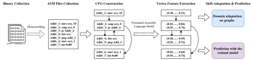
Figure 1: Overview of our approach: we show assembly code on the left and corresponding control flow graph on the right.

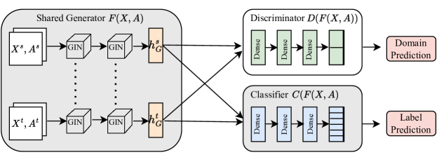
Figure 2: The inputs are source and target graph data, represented as node attribute matrix ($X^{s/t}$) and adjacency matrix ($A^{s/t}$). We can obtain those two matrices for each graph after the Vertex Feature Extraction step in Figure 1. The training process is modeled a minimax game between the generator and the discriminator. $h^{s}_{G}$ and $h^{t}_{G}$ denote the graph-level representations corresponding to the source and target inputs, respectively. Following the training process, the discriminator fails to discern the domain distinction solely based on $h^{s}_{G}$ and $h^{t}_{G}$. At the same time, they retain useful information crucial for achieving good classification on the both domains.

III-C CFG construction from disassembly

We first disassemble binaries file using IDA Pro. We use the open-source code from MAGIC [50] for CFG extraction. The algorithm employs a two-pass traversal methodology, which reads an .asm file as input and outputs the control flow graph. Initially, the file is processed to create a mapping from addresses to instructions. Instructions are associated with four tags, i.e., {start, branchTo, fallThrough, return}, which are used by the second pass. In the first pass, each instruction is visited and its associated tags are updated accordingly. The second pass is dedicated to creating basic blocks and edges between these blocks based on the assigned tags.

III-D Vertex feature extraction

To apply deep learning the CFGs, the first step is to extract feature vectors for the instructions as graph neural networks cannot directly operate on raw instructions. Among the available options – directly feeding raw bytes, employing manually designed features, or automatically generating vector representations for individual instructions using a designated representation model – the preference is given to the third option. This choice yields better quality embeddings without having to manually choose the features. PalmTree [24] is a pre-trained assembly language model based on BERT for general-purpose instruction representation learning. Experiments results in [24] show its efficacy in generating high-quality instruction embeddings for various downstreaming binary analysis tasks such as binary similarity detection, function type signatures analysis, and value set analysis. Hence, we use PalmTree model with pre-trained parameters to generate instruction embeddings.

III-D1 Normalization

In NLP, the Out-of-Vocabulary (OOV) problem occurs when a token encountered during inference is not present in the vocabulary that the model was trained on. The OOV issue in assembly code encoding can be particularly challenging given the diverse nature of codebases and the potential for encountering unseen strings and constant numbers. In order to overcome this, our initial step involves normalizing the CFG: strings are substituted with a designated token [str]. Constants, which contain a minimum of five hexadecimal digits, are substituted with a specific token, [addr]. Smaller constants remain intact and are encoded as one-hot vectors. These strategies align with those utilized during the training of PalmTree.

III-D2 Node feature embedding

After normalization, we apply the PalmTree model to generate a embedding for each instruction. We still need to aggregate vectors in order to obtain a single feature vector to be associated with a vertex. We consider an efficient yet effective solution based on an analysis of the related literature [28]: we aggregate all the instruction embeddings and compute an unweighted mean vector. This process is repeated for all basic blocks, ultimately yielding the final CFG. Each processed CFG is stored by $G=(X,A,Y)$ where $X\in\mathbb{R}^{n\times m}$ is the the node attribute matrix for $G$ with $n$ being the number of nodes and $m$ being the dimension of each node feature vector, $A\in\mathbb{R}^{n\times n_{i}}$ being the adjacency matrix, and $Y$ being the one-hot encoding of the label for $G$.

III-E Shift adaptation: model design

III-E1 Representation learning

Learning with graph data, requires effective representation of their graph structure and node attributes. Graph Neural networks are an effective framework for representation learning of graphs. GNNs generally adopt a recursive aggregation approach where each node combines features vectors of its neighbours to derive its its updated feature vector. With $k$ iterations of aggregation, a node is represented by a node feature vector, encapsulating the structural information within its k-hop neighbourhood. The graph-level representation is achieved via a pooling function. Formally, the k-th iteration of a GNN is constructed as:

$$h_{v}^{(k)} =\text{COMBINE}\left(h_{v}^{(k-1)},a_{v}^{(k)}\right)$$ (1)

$$a_{v}^{(k)} =\text{AGGREGATE}\left(\left\{h_{u}^{(k-1)},\forall u\in\mathcal{N}(v)\right\}\right)$$ (2)

where $h_{v}^{(k)}$ is the feature vector of node $v$ at the $k$-th iteration. We initialize $h_{v}^{(k)}=x_{v}$, where $x_{v}$ is the feature vector for node $v$. $a_{v}^{(k)}$ stands for the aggregation of features vectors from $v$’s neighbours at the $(k-1)$-th iteration. $\mathcal{N}(v)$ are the neighbours to $v$. The selection of AGGREGATE and COMBINE differs among GNN variants. In Graph Isomorphism Network (GIN) which we use in this work, these steps are integrated as follows:

$$h_{v}^{(k)}=\text{MLP}\left(\left(1+\epsilon^{(k)}\right)h_{v}^{(k-1)}+\sum_{u\in N(v)}h_{u}^{(k-1)}\right)$$ (3)

where $\epsilon$ represents a learnable parameter. We designate $\epsilon$ as 0, a configuration referred to as GIN-0 in [49].

The graph representation $h_{G}$ is obtained by aggregating node features from the final iteration $K$:

$$h_{G}=\text{READOUT}\left(\{h_{v}^{(K)}|v\in G\}\right)$$ (4)

READOUT can be a summation function or a graph-level pooling function. There is an important observation about the graph-level readout [49] . Solely relying on the node representations from the final layer might limit the performance as features from earlier iterations may sometimes generalize better. Rather than relying solely on node representations from the last layer, we adopt a concept akin to Jumping Knowledge Networks. In this approach, we concatenate graph representations across all iterations:

$$h_{G}=\text{CONCAT}\left(\text{READOUT}\left(\{h_{v}^{(k)}|v\in G\}\right)|k=0,1,...,K\right)$$ (5)

In the next section, we show the loss function designed to obtain graph representation $h_{G}$.

III-E2 Loss functions

A main goal for the successful domain adaptation is to generate a domain-independent representation of the data from different domains, that is, the representations of graph ($h_{G}$) from the source domain that are similar to those from the target domain. This allows a classifiers trained on graphs from the the source domain to generalize to the target domain as the inputs to the classifier are invariant with respect to the domain of origin. To generate such representation, we leverage the domain adversarial training approach [20, 11] that adversarially trains two neural networks to ensure that the representation is domain invariant. Those two networks serve as a discriminator and generator, respectively. The generator is trained in an adversarial manner to maximize the loss of the discriminator. To learn distinctive graph representations for classification, the generator is also trained with a label predictor.

More specifically, the source inputs is given by $\{({X^{s}_{i}},{A^{s}_{i}},{Y^{s}_{i}},d^{s}_{i})\}$, where each element represents node matrix, node adjacency matrix, class label, and domain label. Target is given by $\{({X^{t}_{i}},{A^{t}_{i}},{Y^{t}_{i}},d^{t}_{i})\}$. The domain label $d_{i}\in\{0,1\}$ is the ground truth domain label for sample $i$. Let $F(X,A;\theta_{f})$ be the generator parameterized by $\theta_{f}$ which maps a node adjacency matrix $A$ and a node attribute matrix $X$ to a hidden graph representation, $h_{G}$, representing graph features that are common across domains. Let $D(h_{G};\theta_{d})$ be the discriminator which maps a hidden representation $h_{G}$ to the domain-specific prediction. Finally, $C(h_{G};\theta_{c})$ represents a classifier, parameterized by $\theta_{c}$ that maps from a hidden representation $h_{G}$ to the task specific prediction. The resulting model is shown in Figure 2.

Inference in our model is given by $\hat{Y}=C(F(X,A;\theta_{f});\theta_{c})$ and $\hat{d}=D(F(X,A;\theta_{f});\theta_{d})$ where $\hat{Y}$ is label prediction and $\hat{d}$ is the domain prediction. The goal of training is to minimize the following loss with respect to parameters $\theta_{f},\theta_{c},\theta_{d}$:

$$min_{\theta_{f},\theta_{c}} \{\gamma\mathcal{L}_{g}+\mathcal{L}_{c}\}$$ (6)

$$min_{\theta_{d}} \{\mathcal{L}_{d}\}$$ (7)

where $\gamma$ is the weight that control $\mathcal{L}_{g}$ term. The classification loss $\mathcal{L}_{c}$ trains the model to predict the output labels. Because we assume the target domain has limited labels, the loss is applies to both domains and it is defined as follows:

$$\mathcal{L}_{c}=-\sum_{i=1}^{N_{s}}{Y}_{i}^{s}\cdot log\hat{Y}_{i}^{s}-\lambda\sum_{i=1}^{N_{t}}{Y}_{i}^{t}\cdot log\hat{Y}_{i}^{t}$$ (8)

where $N_{s}$ represents the number of samples from the source domain, $\hat{Y}_{i}^{s}$ is the softmax output of the model: $\hat{Y}_{i}^{s}=C(F(X^{s}_{i},A^{s}_{i}))$. $N_{t}$ represents the number of samples from the target domain, $\hat{Y}_{i}^{t}$ is the softmax output of the model: $\hat{Y}_{i}^{t}=C(F(X^{t}_{i},A^{t}_{i}))$. We use $\lambda$ as the penalty coefficient for the loss value obtained from target data.

The discriminator loss trains the discriminator to predict whether the output of $F$ is generated from the source or the target domain. Let $\hat{d}_{i}^{s}=D(F(X^{s}_{i},A^{s}_{i}))$ and $\hat{d}_{i}^{t}=D(F(X^{t}_{i},A^{t}_{i}))$ be the domain predictions from sample of source and target respectively. The discriminator loss is also applied to both domains and it is defined as follows:

$$\mathcal{L}_{d}=-\sum_{i=1}^{N_{s}+N_{t}}\left[{d}_{i}log\hat{d}_{i}+(1-{d}_{i})log(1-\hat{{d}}_{i})\right]$$ (9)

Finally, the generator loss encourages the hidden graph representations $h_{G}^{s}$ and $h_{G}^{t}$ from the generator to be as similar as possible so the discriminator can not predict the domain of the representation. This is achieved via adversarially training the generator so that parameters $\theta_{f}$ are optimized to reduce the domain classification accuracy. Essentially, we minimize the loss for domain prediction task with respect to $\theta_{d}$, while maximize it with respect to $\theta_{f}$. Hence, the generator loss is defined with inverted ground truth domain labels:

$$\mathcal{L}_{g}=-\sum_{i=1}^{N_{s}+N_{t}}\left[(1-{d}_{i})log\hat{d}_{i}+d_{i}log(1-\hat{{d}}_{i})\right]$$ (10)

III-E3 Model training

Training $F$ consists of optimizing $\mathcal{L}_{g}$ and $\mathcal{L}_{c}$, since we want to minimize the domain classification accuracy and maximize label classification accuracy. The discriminator is trained with $\mathcal{L}_{d}$ to maximize domain classification accuracy. The classifier is trained with $\mathcal{L}_{c}$ to maximize label prediction accuracy. The training algorithm follows the mini-batch gradient descent procedure. More specifically, the following steps are executed after creating the mini-batches. The generator updates their weight to minimize $\gamma\mathcal{L}_{g}+\mathcal{L}_{c}$. The classifier updates its weight to minimize classification loss. The discriminator weights remain frozen during this step. Then, the discriminator updates its weight to minimize discriminator loss. Upon the model’s convergence, we are able to achieve graph representations that are both discriminative of the class and invariant to the domain. To classify graphs in the target, one can obtain prediction by running $C(F(X,A))$.

IV Generating drifted malware clusters

Previously malware drift analyses have evaluated their approaches by designing experiments on existing malware datasets. Despite varying experiment designs, all of them rely on the original family labels of malware for their analyses. In this paper, we do so as well. However, we discovered that despite being labeled as different families, malware samples exhibit highly similar characteristics in one of the mostly used benchmarks. This phenomenon is evidenced the data in Table I, which shows that the distances between malware samples from different families are remarkably small. Evaluation relying on those family labels is likely to overestimate the prediction accuracy. Consequently, we developed and implemented a graph-based clustering algorithm to assign cluster labels to malware, thereby increasing inter-cluster distance and amplifying domain shift. Our assessment is conducted in two scenarios to demonstrate the effect of performance overestimation: one evaluation using the initial labels and another using the labels from clustering.

Evaluation based on original labels. The evaluation was conducted using the original labels of the dataset. We employed the “leave-one-out” approach, where we designated one family label as the target domain and treated the remaining family labels as the source domain.

Evaluation based on cluster labels. We assign new labels to the samples using the graph clustering approach detailed below. Then we apply the same “leave-one-out” method. This task is more difficult due to the significantly increased distances between clusters compared to those with the initial labels, as shown in Table I.

IV-A Graph clustering algorithm

The graph clustering algorithm comprises two primary components: (1) the graph embedding component, responsible for learning a feature vector at the graph level, and (2) a weighted consensus clustering mechanism that operates on the learned graph embeddings using an ensemble of clustering predictors. The resulting clusters are generated via a weighted consensus method that takes into account the performance of every single predictor.

IV-A1 Graph embedding

The goal is to learn a graph representation able to preserve the graph structure and code semantics. The representations learned by minimizing Equation 6 are not suitable for this task since they only contain information that is helpful for classification, and will filter out other information that is important for capturing the characteristic of the entire graph. Therefore, we consider solutions based on graph autoencoder (GAE) [36, 18], which consists of an encoder that learns a hidden representation and a decoder that is able to reconstruct the entire graph from this representation. Our implementation of this model involves utilizing a graph convolutional network (GCN) as the encoder and a simple inner product as the decoder.

In particular, we calculate graph embedding $Z$ and the reconstructed adjacency matrix $\hat{A}$ as follows:

$$\hat{A}=\sigma(ZZ^{\top}),\ Z=GCN(X,A)$$ (11)

where $\sigma(\cdot)$ is the sigmoid function. We use binary cross entropy loss for reconstruction loss which is used to train both encoder and decoder.

$$\mathcal{L}_{\mathit{recon}}=\mathit{-\sum_{i,j}\left[A_{ij}log(\hat{A}_{ij})+(1-A_{ij})log(1-\hat{A}_{ij})\right]}$$ (12)

where $\mathit{A_{ij}}$ is 1 if there is an edge between node $i$ and $j$, and 0 otherwise. After training the graph autoencoder with $\mathcal{L}_{\mathit{recon}}$ on graph $G=(X,A)$, we derive the graph representation $Z$ from the encoder: $Z=GCN(X,A)$, and then retrain the graph autoencoder from scratch for the next graph to get its graph representation.

IV-A2 Weighted consensus clustering

After obtaining an embedding for each graph, the next step is to assign a new label to each graph based on unsupervised clustering. In this paper, we introduce a novel weighted consensus clustering approach that leverages multiple clustering algorithms and assigns more weight to predictors that yield better clustering results.

First, we apply $P$ distinct clustering algorithms to the graph embeddings, resulting in $P$ individual clustering solutions. Each solution assigns every graph to a specific cluster. In total, we have $P$ label solutions plus the original label if available. Next, we initialize a consensus matrix $\mathit{CM}$ with zeros. We iterate through all the solutions and update the consensus matrix on the fly. For every pair of graphs $i$ and $j$, if $i$ and $j$ belong to the same cluster, we update the matrix $CM$ using the formula:

$$\mathit{CM[i][j]\mathrel{+}=1\times\frac{(s-(-1))}{2}}$$ (13)

Here, $s$ denotes the silhouette coefficient of the current clustering solution, which is the mean of the silhouette coefficient for all samples. The silhouette coefficient for one sample is given as $\mathit{\frac{b-a}{max((a,b))}}$ [35], where $a$ is the mean distance between a sample and all the others in the same cluster and $b$ is the mean distance between a sample and all other samples in the nearest cluster. The averaged silhouette coefficient ranges from $-1$ for incorrect clustering to $+1$ for well separated clustering. A superior clustering solution, characterized by a higher silhouette score, exerts a higher coefficient ($s$), hence a greater impact on the $CM$ matrix. Finally, we apply a final clustering algorithm to the normalized consensus matrix to derive the ultimate clusters, assigning each graph a new cluster label.

V Evaluation: Unseen Malware Family

In this section, we evaluate our approach using two popular Windows malware benchmarks: Microsoft malware classification challenge (Big-15) and MalwareBazaar dataset (MalBaz). We focus on the evaluation of detecting previously unseen malware. For each dataset, our assessment is conducted in two scenarios: one with the original labels and another using the labels generated by our graph cluster algorithm. We will evaluate different malware representation and current retraining approaches for each representation in Section VI. Finally, we evaluate the in-class malware drift where the task is in the classification of multiple malware families that have evolved over time (Section VII).

V-A Evaluation based on original labels of Big-15

V-A1 Dataset

The Microsoft Malware Classification Challenge (Big-15) [34] is one of the mostly used benchmarks for testing malware classification methods. In total, it has $21,741$ malware samples where $10,868$ samples are labeled. Those labeled samples are from nine different malware families, namely Ramnit, Lollipop, Kelihos_ver3, Vundo, Simda, Tracur, Kelihos_ver1, Obfuscator.ACY, Gatak. Each sample consists of a .byte file, a binary representation of a hexadecimal number, and an .asm file, the disassembly outputs of IDA Pro. Microsoft removed the PE header to ensure file sterility. In this experiment, we created CFGs from $10,868$ .asm files.

Since Big-15 does not have benign samples, we select two different benign binary datasets: BinaryCorp-3M [45] and benign Windows PE files. BinaryCorp-3M consists of binaries from the official ArchLinux packages and Arch User Repository. The repository includes packages for editor, instant messenger, HTTP server, web browser, compiler, graphics library and cryptographic library. The dataset includes $8,357$ binaries compiled with gcc and g++ with different optimization levels. From the BinaryCorp-3M train, we obtained $6,392$ assembly files successfully using IDA Pro. Benign Windows PE files are taken from installed folders of applications of legitimate software from different categories. In total, we successfully disassembled $1,000$ Windows PE files for our experiment.

V-A2 Source and target datasets setup

As is typical for research on combating drift in malware [51], we employ the “leave-one-out” strategy to simulate an unseen malware family. We pick one of the malware family as the previously unseen family (serve as the target malware data), the remaining families as the source malware data. We ensure the general applicability of our results by repeating this process with Ramnit, Lolipop, and Kelihos_ver3, the dataset’s top three malware families.

Both the source and the target datasets contains benign samples. BinaryCorp-3M is used as the benign data for source domain, while the target domain uses benign Windows PE binaries. We utilize distinct benign datasets in the source and target domains because benign software can have concept drift as well. BinaryCorp provides a larger set of $48,130$ binaries. However, when we exclude one family, the source domain malware data will be around $8,000$. To prevent class bias from an extremely imbalanced dataset, we opt not to use the larger version of BinaryCorp. Instead, we use $6,392$ samples from BinaryCorp-3M as the benign data in the source dataset, achieving an approximate malware-to-benign ratio of $1.3:1$ in all experiments. The unseen family is combined with $1,000$ benign Windows applications to form the target dataset, maintaining an approximate malware-to-benign data ratio of $1.8:1$.

The source and target datasets are then split into source training set ($75\%$), source testing set ($25\%$), target training set ($50\%$) and target testing set ($50\%$), respectively. To prevent bias, the malware/benign class ratio is consistent across training and testing sets in all domains. Our model is trained using the labeled source training set and a subset of the labeled target training set, then evaluated on the target testing set, which is unavailable during training. In continuous learning, the concept of labeling budget allows for a finite number of new samples to be labeled by analysts. We emulate this by randomly selecting $20,50,100,200,300,500$ labels from the target training set and use them as the target data for training. The objective is to accurately detect malware samples in the target testing set using as few target labels for training as possible.

V-A3 Baselines

We evaluate our scheme against existing graph-based malware classification methods and several enhanced baselines, which are adapted from previously published work with our improvements. This allows us to demonstrate evidence that our method outperforms all these approaches.

Current methods. MAGIC [50]: Yan et al. [50] developed MAGIC, employing DGCNN, a type of GNN, to classify CFGs with basic blocks serving as nodes. MAGIC utilizes manually crafted token-level and block-level features to represent each basic block. Table V in the Appendix shows the features defined in MAGIC.

MCBG [46]: MCBG is another CFG-based malware classification model. MCBG adopts pre-trained BERT model to produce node embeddings instead of relying on handcrafted features like MAGIC. They also adopted GIN for the classification model.

For all the current methods, we use cold start learning (i.e. we train a classifier from scratch with target training labels), consistent with past work. We directly adopt their public available implementations with default hyper-parameter. The details can be found in Appendix -A2.

Improved baselines. Warm start MAGIC and MCBG: We extend those works with warm-start learning. Rather than training a new model from scratch each time, we first train the model with the source training data and continue training it with target training samples. The details of implementation and retraining procedure can be found in Appendix -A2.

DAN [25]: DAN was originally designed to generalize deep convolutional neural network to domain adaptation with images. Specifically, it learns a domain-independent representation by reducing the discrepancy in domain distribution. This discrepancy is quantified using the Maximum Mean Discrepancy (MMD) loss. We adapt DAN to support graph-based malware classification models. It learns a domain-independent graph representation via a shared feature extractor, which is based on GIN. Subsequently, we implement a classifier that uses this graph representation as input to determine if it is a malware. The feature extractor is trained to minimize both the classification loss and the MMD loss, while the classifier is trained to minimize the classification loss. The MMD loss is computed using the hidden graph representations $h_{G}^{s}$ and $h_{G}^{t}$ derived from the feature extractor. We opt for RBF as kernel functions, following previous studies. To ensure a fair comparison, the architecture of the feature extractor and classifier mirrors that of the generator and classifier components in our method. Please see Appendix for the detailed implementation of DAN -A2 and our approach -A1.

Figure 3: Given a fixed target training labels, we compute the average accuracy on the target testing data for different baseline techniques and our method. The top three figures are evaluated on the target family based on original labels of Big-15, the bottom three figures are for the cluster labels.

V-A4 Results

We conduct each experiment five times and compute the average results across all five iterations. The accuracy on the three target family are presented in the top three graphs in Figure 3. The f1 score can be found in Table VII located in the Appendix.

We observe:

• Our approach has the best accuracy in all experiments. It achieves over 94% accuracy when only trained with 20 labeled samples from the target, demonstrating that our adaptation approach can effectively adapt to new malware family with very few labels.

• DA methods (including DAN MMD and Ours) perform better than the warm-start learning strategy, while the cold start training yields the least effective results when trained with the same amount of target labels.

• The warm-start learning strategy outperforms the cold-start one due to pre-training on a larger dataset with other malware families.

• When the target family is Kelihos_v3, the MCBG (Warm) and MAGIC (Warm) method attains 94% accuracy with just 50 samples, This is primarily due to the lack of clear separation among different family labels, resulting in a small domain shift between source and target data.

In the next experiment, we initially demonstrate that the original labels of Big-15 are not well separated using common inter-label distance metrics, potentially resulting in an overestimation of the warm-start learning and DA methods. To this end, we create denser clusters for the same dataset using the graph-based clustering algorithm presented in Section IV-A and evaluate all the methods on this more challenging adaptation task.

V-B Evaluation based on cluster labels of Big-15

V-B1 Inter-label distance metrics

We refer to three common metrics to measure the distance among labels, i.e., Sihouette Coefficient [35], Calinski-Harabasz Index [6], and Davies-Bouldin Index [10]. Those three metrics respectively measure if clusters are dense and well separated. The Calinski-Harabasz index is defined as the ratio of the between-clusters dispersion and the within-cluster dispersion where dispersion is defined as the sum of distances squared. The score is higher when clusters are dense and well separated. The Davies-Bouldin Index compares the size of the clusters with the distance between clusters. Zero is the lowest possible score. Values closer to zero indicate a better partition.

Those metrics aren’t directly applicable to graphs. We use the method from Section IV-A to learn graph embeddings, compute metrics from transformed vectors and original labels, and present results in Table I. All three metrics indicate that the samples with different labels are not well separated. We transformed the graph feature vectors using T-SNE to give a visual insight on the poor partition of data based on the original label. The visualization is shown in Figure 4.

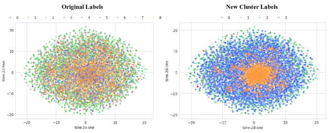
Figure 4: Visualization of the graph feature vector with their labels. The left one shows the data with original labels from Big 15 [34], the right one shows the newly learned clusters. The legend represents the mapping between labels and colors.

TABLE I: Evaluation of the original labels and new clusters of Big-15 with distance-based metrics. All metrics confirm that our new clusters better separate data, with distant samples in different clusters and close samples within the same cluster.

Metric	Original labels	New clusters
Silhouette Coefficient	-0.112	-0.036
Calinski-Harabasz Index	0.540	61.150
Davies-Bouldin Index	40.210	29.511

V-B2 Obtaining well-separated clusters

We implemented the graph clustering algorithm in Section IV-A to obtain the new cluster labels for Big-15. First of all, we trained a graph autoencoder to derive a 256-dimensional feature vector for each malware graph. In the consensus clustering algorithm, we applied three different clustering predictors: Gaussuan Mixture Model (GMM), HDBSCAN, and K-means. For each predictor, we followed the best practice for selecting the parameters. For K-means clustering, a heuristic approach based on inertia values was utilized to determine the appropriate cluster number. In the case of GMM, all combinations of six components and four covariance types were explored to identify the model with the lowest Bayes Information Criterion. Regarding HDBSCAN, parameters were set to $min\_cluster\_size=2$ and $min\_samples=2$ to reduce the number of outliers. During the consensus matrix update, all three clustering solutions along with the original labels were considered. Finally, the GMM model was utilized to derive the ultimate clusters for our analysis. Figure 4 illustrates the new clusters, while Table I presents the metric values for the new labels. All three metrics confirm that our new clusters better separate data.

V-B3 Source and target datasets setup:

We still employ the “leave-one-out” strategy and pick one of the cluster label as the “unseen family” and the remaining clusters as the source malware data. We still use the BinaryCorp-3M as the benign data for the source and benign Windows PE for the target. The train/test split ratio for each domain remain consistent with those detailed in Section V-A2.

V-B4 Results

TABLE II: Impact of more accurate labels on various training strategies . The tables shows the difference in average accuracy, determined by the original and cluster label assignment. A positive value indicates an enhancement in performance relative to the original label, while a negative value signifies a decline.

Strategy	Method	Target samples
		20	50	100	200	300	500
Cold	MCBG	0.3	0.2	-0.4	-0.2	0	0.2
	MAGIC	0.1	0.4	0.2	-0.1	0.3	0.3
Warm	MCBG	-3.4	-4.9	-5	-2.2	-0.5	0.3
	MAGIC	-0.8	-2.2	-3.7	-1.7	-1.5	-2.4
DA	DAN (MMD)	-0.6	-2	-0.8	-1.5	-0.2	-0.1
	Ours (Adv)	-1.7	-1.3	0.2	-0.9	-0.3	-0.3

We implement the same baselines as in the previous experiments. Similarly, we conducted three adaptation tasks, each targeting a specific cluster. We randomly sampled 20, 50, 100, 200, 300, 500 labels from the target training set for each task. The accuracy on the target testing set are presented in the bottom three graphs in Figure 3. The f1 score can be found in Table VIII in the Appendix. To understand the impact of the more accurate labels on different training strategies, we obtained the averaged accuracy of each approaches based on original label and cluster label, calculated the difference, and show the results in Table II. The highlight results are:

• Our approach maintains the highest accuracy across all experiments and demonstrates robust performance even in this more challenging adaptation task. It achieves an average accuracy of 92% when trained with only 20 labeled samples from the target domain.

• In a repeated observation, the DA methods yield the highest performance, with warm-start learning trailing behind, and cold-start learning producing the lowest outcomes.

• Warm-start strategies have experienced the most substantial performance decline due to a more pronounced distribution shift between the source and target domains. When assessed on actual drifted labels, MCBG (Warm) saw an average accuracy decrease of $2.6\%$. Similarly, MAGIC (Warm) experienced an average accuracy decrease of $2.1\%$.

• The DA methods’ performance has seen a minor decline. Specifically, DAN’s average drop was $0.86\%$, while our method experienced the smallest drop of $0.72\%$

• As expected, cold-training performs similarly since it only sees the target data, but not the source data.

V-C Evaluation based on the cluster labels of MalwareBazaar

MalwareBazaar (MalBaz) is a more recent dataset that includes the top-6 malware families in 2020. After filtering out samples that are not in PE format and further leverage multiple anti-virus engines to remove the noisy samples that have inconsistent labels, Ma et al. [26] obtained $3,971$ malware samples from 6 families in total. From the MalBaz dataset, we obtained $3,000$ assembly files successfully using IDA Pro.

MalBaz has the lastest malware samples which may provide a different perspective and complement with Big-15. We first measure original labels of MalBaz using the same distance-based metrics. We found that the original labels of MalBaz already have better scores than Big-15. This is likely due to the fact that each sample in MalBaz was assessed using various AV engines, all of which provide consistent labels. Nevertheless, we performed our graph-based clustering algorithm and the cluster labels we generated still demonstrate a better score across all metrics.

We repeat the same experiments on the original and clustering labels of MalBaz. The configuration of the source and target datasets mirrors that of Big-15, with the only difference being that MalBaz has fewer malware data. To ensure that the ratio of malware to benign data is not excessively skewed which would introduce additional bias, we adjusted the quantity of benign data in both domains accordingly so that the amount of benign samples is similar to the amount of malware samples. We employed the same baselines, and the specifics of each baseline’s implementation can be located in Appendix -B2.

The results of the averaged accuracy based on cluster labels is shown in Figure 5 while the results for the original labels is in Figure 8 in the Appendix. Our approach demonstrates superior performance in predicting unseen malware on MalBaz as well. Given that the original labels are more distinctly separated than in Big-15, we notice a smaller decline in performance with warm-training strategies when evaluated on the clustering labels.

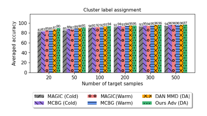
Figure 5: Averaged accuracy on the target testing data for different techniques. The evaluation is based on the cluster label of MalwareBazaar.

VI Evaluation: Impact of Different Representations

In this section, we conduct a comprehensive analysis on the effectiveness of various combinations of malware representation with diverse model update tactics. We consider the existing cold-start and warm-start learning approaches, as well as novel approach grounded in domain adaptation. Our objective is to answer the following research questions:

Q1: How effective is our adaptation technique when dealing with different malware representations, such as those that are content-based or image-based? Is this the best method for updating the model using these two representations?

Q2: Does our graph representation contributes to the overall model’s performance? If so, to what extent?

Q3: In terms of cold-start and warm-start learning, which form of malware representation is more effective?

To answer those questions, we use the Big-15 dataset, obtained three representations (content-based, image-based, graph-based) for each malware sample, and tested with various baselines proposed by literature for each representation. For the malware data, we use the new cluster label as it poses a more challenging adaptation task. The configuration of the source and target datasets adheres to the same process outlined in V-A2 and remains consistent across all representations. In what follows we first describe the representation we consider. Then we discuss the implemented baselines for each representation, followed by the results of our evaluation.

VI-1 Content-based features and baselines

We select nine families of static analysis features that were curated in prior research works [1, 2]. In total, we extracted total of 965 individual features from the assembly code sample in our datasets. A brief summary of the features is listed in Table III while a comprehensive explanation is included in Appendix -C.

TABLE III: Nine family of features extracted based on the content of assembly file.

Feature Type	Feature Description
Symbol	Frequencies of special symbols
Opcode	Frequency of common opcodes
Register	Frequency of registers
Windows API	Frequency of use of Windows APIs
Section	Statistical attributes that capture the proportion of each section
Data Define	Statistical features that summarize the characteristics of data definition instructions
Others	File size and the number of lines

Current methods. SVM and MLP in both cold and warm settings: In continuous learning for malware detection, SVM and MLP is a commonly used classifier model to learn from tabular features extracted from malware samples [51, 7]. Chen et al. [7] further enhanced this approach by incorporating warm-start training, which they found to be superior to cold start for malware detection models. The details of each classifier can be found in Appendix -D.

Improved baselines. DAN: We modify DAN to accommodate MLP-based models for malware classification. Both the feature extractor and the classifier are implemented as neural networks, and their combined structure mirrors the layer configuration of the baseline MLP. The feature extractor is trained to minimize both the classification and MMD losses, while the classifier’s training focuses on minimizing the classification loss. The computation of the MMD loss involves the hidden representations obtained from the feature extractor. Consistent with prior research, we choose RBF for kernel functions.

For our adaptation method, to maintain an equitable comparison, we have designed the architecture of the generator and classifier to be the same as the structure of the feature extractor and classifier modules in DAN. The key distinction is that our domain representation is acquired via adversarial learning loss in Equation 6 and 7, not through MMD loss. Please see Appendix -D for the detailed implementation of DAN and our approach.

VI-2 Image-based features and baselines

We adopt the same approach as in [42, 26, 4] to transform a malware binary into an image. This method does not require any feature engineering and domain expert knowledge. It reads a given binary as a vector of 8-bit unsigned integers and then converts a vector into a 2D array. The height of the malware image is allowed to vary depending on the file size, and the width of the malware image is fixed. We apply this process to our datasets to obtain images of binaries.

TABLE IV: Accuracy of baselines across various malware representations. In terms of content and image representation, we illustrate the percentage change in accuracy from our adversarial (Adv) DA method to the peak performance among all baselines within the same representation. Ultimately, we demonstrate the enhancements of our full pipeline (graph + Adv DA) compared to both content + Adv DA and image + Adv DA.

			Cluster 0: target samples						Cluster 1: target samples						Cluster 2: target samples
Malware Representation	Strategy	Method	20	50	100	200	300	500	20	50	100	200	300	500	20	50	100	200	300	500
		SVM	79.1	83.3	84.1	88.7	90.8	93.0	73.6	75.5	78.1	84.7	88.9	90.1	80.0	83.2	88.0	90.3	96.2	97.6
	Cold	MLP	82.4	85.1	90.7	91.6	94.2	96.3	73.8	79.3	82.4	89.9	90.9	95.8	80.4	84.0	88.3	91.8	96.7	97.3
		SVM	82.4	83.5	89.7	91.0	91.8	93.5	75.4	77.3	79.6	86.1	89.0	90.2	81.0	85.2	89.0	95.5	98.0	99.2
	Warm	MLP	84.2	87.9	91.1	93.6	95.7	96.9	82.2	87.7	86.5	92.1	94.0	95.6	81.8	85.8	89.2	96.5	98.6	99.2
		DAN (MMD) + MLP	85.9	89.4	90.2	93.5	94.7	97.0	82.2	87.7	86.5	92.1	94.0	95.6	80.5	85.8	89.2	96.5	98.0	99.0
			87.3	90.2	93.5	94.0	95.7	96.9	85.0	89.8	90.0	93.9	95.0	95.9	83.0	87.4	90.7	96.5	98.8	99.0
Content-based (CB)	DA	Ours (Adv) + MLP	$\uparrow$1.4	$\uparrow$0.8	$\uparrow$2.4	$\uparrow$0.4	$\uparrow$0	$\downarrow$0.1	$\uparrow$2.8	$\uparrow$2.1	$\uparrow$3.5	$\uparrow$1.8	$\uparrow$1.0	$\uparrow$0.1	$\uparrow$1.2	$\uparrow$1.6	$\uparrow$1.5	$\uparrow$0	$\uparrow$0.2	$\downarrow$0.2
	Cold	ResNet-50	50.3	50.3	75.5	89.2	90.9	92.1	49.9	54.3	65.0	76.8	88.2	91.3	49.5	60.7	67.5	71.5	81.8	86.4
	Warm	ResNet-50	89.0	90.0	91.5	93.1	94.9	96.3	79.6	84.5	85.0	91.4	94.2	94.8	81.6	83.4	89.4	90.4	90.5	94.6
		DAN (MMD) + CNN	89.4	90.3	91.7	93.3	94.0	96.0	86.0	89.5	90.9	92.6	94.2	94.6	85.1	86.2	89.8	90.6	91.4	94.4
			89.6	92.6	94.2	93.3	95.3	96.5	90.7	92.0	93.1	94.3	94.5	95.3	86.9	87.0	90.3	91.3	93.6	94.4
Image-based (IB)	DA	Ours (Adv) + CNN	$\uparrow$0.2	$\uparrow$2.3	$\uparrow$2.5	$\uparrow$0	$\uparrow$0.4	$\uparrow$0.2	$\uparrow$4.7	$\uparrow$2.5	$\uparrow$2.2	$\uparrow$1.7	$\uparrow$0.3	$\uparrow$0.5	$\uparrow$1.2	$\uparrow$0.8	$\uparrow$0.5	$\uparrow$0.7	$\uparrow$2.2	$\uparrow$0
Graph-based (GB)	DA	Ours (Adv) + GIN	93.5	95.8	98.1	97.4	99.4	99.6	93.1	95.8	99.3	99.8	99.5	99.6	91.4	93.7	99.5	99.7	100	100
Improvement over CB: Ours (Adv)			$\uparrow$6.2	$\uparrow$5.6	$\uparrow$4.6	$\uparrow$3.4	$\uparrow$3.7	$\uparrow$2.7	$\uparrow$8.1	$\uparrow$6	$\uparrow$9.3	$\uparrow$5.9	$\uparrow$4.5	$\uparrow$3.7	$\uparrow$8.4	$\uparrow$6.3	$\uparrow$8.8	$\uparrow$3.2	$\uparrow$1.2	$\uparrow$1
Improvement over IB: Ours (Adv)			$\uparrow$3.9	$\uparrow$3.2	$\uparrow$3.9	$\uparrow$4.1	$\uparrow$4.1	$\uparrow$3.1	$\uparrow$2.4	$\uparrow$3.8	$\uparrow$6.2	$\uparrow$5.5	$\uparrow$5	$\uparrow$4.3	$\uparrow$4.5	$\uparrow$6.7	$\uparrow$9.2	$\uparrow$8.4	$\uparrow$6.4	$\uparrow$5.6

Current methods. Cold-start ResNet-50: We follow the previous works, which uses several deep convolutional neural networks for malware prediction. We choose to implement the network components as ResNets-50 with short-cut connections since it shows the best prediction performance with images of malware [26]. In our first baseline, we train a ResNet-50 model from scratch using only target training samples, following approaches in [31, 38] where no adaptation is involved. The implementation and training details can be found in Appendix -E.

Warm-start ResNet-50: This approach aligns with the predominant methodologies employed in classifying malware images with concept drift  [26, 42, 5, 19]. Specifically, we utilize the same customized ResNet-50 architecture as described earlier, but initialize the model with weights from pre-training on ImageNet. Subsequently, we retrain the model using both source and target image data. This strategy not only leverages the network’s knowledge of general images but also integrates insights learned from the source malware data.

Improved baselines. DAN: Our implementation of DAN and our methodology utilizes a multi-layered CNN, which is less complex than ResNet-50. This demonstrates that the DA techniques surpass both the cold-training and warm-training approaches, even when using smaller models. For an in-depth explanation of the implementation of DAN and our methodology, please refer to Appendix -E.

VI-3 Results

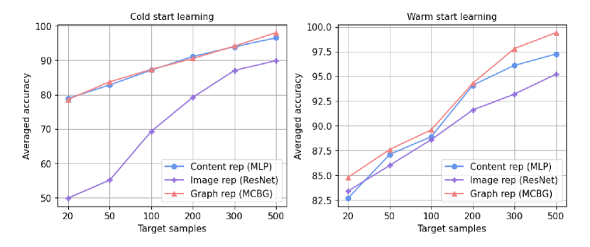
Figure 6: Comparison of different representations under cold start learning (left) and warm start learning (right).

Each baseline is assessed across three adaptation tasks, with each task focusing on a specific cluster. The accuracy of all feature representations alongside their respective baselines is displayed in Table IV. The f1 score can be found in Table XI in the Appendix. We have omitted the cold and warm strategies from the table for the graph representations as they have already been presented in Figure 3. Instead, we have selected the top-performing method from each representation under both cold-training and warm-training settings for a direct comparison in Figure 6. The following are our observations in response to the initial questions:

• The use of our shift adaptation component consistently has the highest accuracy across all feature representations, demonstrating the versatility of adversarial adaptation in accurately predicting new instances of malware (Q1).

• All the key components in our pipeline contribute to the overall model’s performance. Combining the adaptation approach with our graph representations achieves the best results. (Q2).

• In cold start training, content-based and graph-based representation has similar performance while the image model using image features performs poorly, indicating the challenge posed by inadequate training data for large-scale neural network models (Q3).

• In warm start training, image model shows the most improvement, while the graph representation surpasses other representations in most cases (Q3).

VII Evaluation: In-class Evolution

VII-1 Dataset

In this experiment, we use the MalwareDrift dataset [26][43]. The dataset encompasses samples from 7 distinct malware families, namely Bifrose, Creeinject, Obfuscator, Vbinject, Vobfus, Winwebasec, and Zegost, each representing various types of malware such as trojans, worms, adware, and backdoors. Samples within each family are categorized into pre-drift and post-drift segments, with the partition determined at points of significant evolution. The evolution was determined using a ML-based tracking method that trains an SVM on malware families over time windows. The $\chi^{2}$ statistic is employed to quantify variations in SVM weights over these sliding time windows. Significant spikes in the $\chi^{2}$ timeline, indicate alterations in the malware’s characteristics.

Previous work by Ma et al. [26] has shown that models trained on the pre-drift data peforms poorly on the post-drift data. The top graph in Figure 7 shows performance data from  [26] on pre-drift and post-drift testing data for five models trained solely on pre-drift training data. As we can see from the figure, the reduction in accuracy ranges from 23.0% to 38.7%. It is thus clear that all considered models experience a substantial performance decrease when confronted with code evolution within the same malware families.

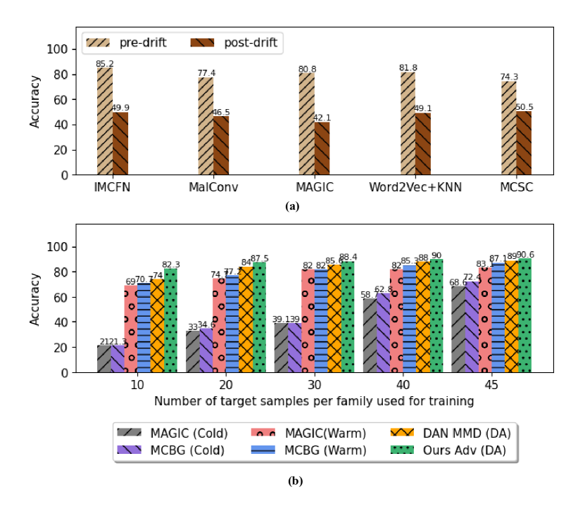
Figure 7: Accuracy of source only approach (a); Accuracy on post-drift data using 10-45 labeled data from each post-drift family (b). Table XII in Appendix shows the f1-score.

VII-2 Source and target data setup

Since the post-drift samples exhibit significant divergence compared to the pre-drift domain, our evaluation utilizes the original labels without the need to run our clustering algorithm for reassigning cluster labels.

The source domain comprises the pre-drift data from 7 families, and the target domain consists of the post-drift data from the same 7 families. Our objective is to train a classifier able of accurately classifying malware families within the post-drift data using limited post-drift labels. We randomly sample ${10,20,30,40,45}$ labeled data from each family in the post-drift dataset to form our target training set while the rest of the samples form the target testing set. We use all of the pre-drift data as the source training set.

VII-3 Baselines

We use the same baselines approach listed in Section V-A3. We include the implementatioon details of each baseline in Appendix -F.

VII-4 Results

The results, presented in the bottom graph of Figure 7, reveal that:

• Our methodology significantly outperforms other baseline methods in all experiments. It achieves an 82.3% accuracy in predicting 7 malware families in the post-drift set with just 10 labeled samples per family, a 30% improvement over training solely with pre-drift data.

• In comparison to other baselines, DAN exhibits superior performance. This reaffirms that domain adaptation is more efficient in updating the model given an equal number of labels.

• MAGIC (Cold) and MCBG (Cold) failed to converge due to insufficient data, especially for complex tasks like multi-class classification.

• MAGIC (Warm) and MCBG (Warm) while not as effective as ours, has a considerate performance boost compared to trained each model in a cold-start setting.

VIII Future work

In this paper, we focus on adapting malware for one system architecture or one instruction set. We have specifically conducted an evaluation of x86, given the notable absence of work pertaining to Windows malware. However, our approaches are applicable to other systems as well, such as Android malware. It is to be noted that we have not conducted tests on packed executables within the scope of this work. It would be of interest to study whether the application of our approach could enhance the detection of malware with unseen packing routines with a minimal number of packed labels. This is an aspect we intend to explore in future work.

IX Conclusion

This paper focuses on the classification of drifted malware, particularly the challenge of model adaptation with scarce labels. To address this issue and establish a foundation for the assessment of adaptive methods, we have introduced a new approach for adapting the model with limited new labels, along with a graph clustering method for creating statistically separate malware clusters.

Our approach is based on adversarial domain adaptation but operates on control flow graphs of malware, exploiting the consistent characteristics of malware in terms of assembly code semantics and control flow execution. Our automated process comprises three main elements: construction of CFGs, extraction of vertex features, and adaptation of shifts. To retain the semantics of the code from the instructions, we utilize an assembly language model to generate high-quality feature embeddings for each instruction within every node. We have designed a set of evaluations to systematically compare our training approach with other approaches from previous published work or adapted to support malware classification. The experimental results show that our approach outperforms others in three distinct adaptation tasks with increasing adaptation complexity: evaluation based on original family labels showing minimal drift, evaluation based on new clusters with significant shift, and classification of multiple malware families that have evolved over time. We also demonstrate that our adaptation component can be used with other malware representations to enhance performance, while our graph representation achieves the best results with very few labels. We conclude that our approach can effectively improve the model performance when trained with scarce new labels.

Acknowledgements. This work has been partially supported by NSF grant IIS 2229876.

-A Implementation details and additional results on unseen family evaluation (Big-15)

-A1 Our model implementation details

We implemented our model using TensorFlow and Spektral, a library for GNN. The generator has 3 GIN layers and ends with a global average pooling, and a dense layer with 256 neurons. The architecture of the classifier consists of 2 fully connected layers (FC_1, FC_OUT). The number of neurons in FC1 is 256. FC_OUT is the output layers for label prediction. The discriminator has two layers with 256 hidden units and is followed by the softmax layer for domain prediction. Batch normalization is applied on every hidden layer. For training the model, we use the Adam optimizer with a learning rate of $\mathit{1e-3}$ for 60 epochs. The batch size is 32. The coefficient of the loss $\mathcal{L}_{g}$ is set to 0.1 , which allows the discriminator to be less sensitive to noisy signals during training. We set $\lambda=0.1$ in $\mathcal{L}_{c}$ since we have much more labeled data from the source.

-A2 Baseline implementation details

MAGIC (Cold): MAGIC utilizes handcrafted features to represent each basic block, which is listed in Table V. The classification model is DGCNN that uses a SortPooling layer. Our DGCNN topology is based on the ones used in [50], to be comparable to previous work. We train the model using Adam optimizer with a learning rate of $\mathit{1e-3}$ for 60 epochs.

TABLE V: Basic block attributes defined in MAGIC

Attribute Type	Attribute Description
token-level	# Numeric Constants
	# Transfer Instructions
	# Call Instructions
	# Arithmetic Instruction
	# Compare Instructions
	# Mov Instructions
	# Termination Instructions
	# Data Declaration Instructions
	# Total Instructions
block-level	# Offspring, i.e., Degree
	# Instructions in the Block

MCBG (Cold): MCBG uses GIN-JK model as the classifier. We use their default GIN-JK model with the same hyperparameters used in [46]. MAGIC is trained using Adam optimizer with a learning rate of $\mathit{1e-3}$ for 60 epochs.

MAGIC (Warm) and MCBG (Warm): In [7], warm-start learning takes an older model and continue training the entire model with new samples. However, we found that freezing the weights of the initial layer of the older model performs better on this dataset so we opted for this approach. In fact, this approach aligns with a commonly used fine-tuning paradigm in transfer learning, where certain layers are frozen to retain the knowledge gained from the source data.

DAN: The network architecture of the feature extractor and classifier is the same as the generator and classifier mentioned in Appendix -A1. The feature extractor has 3 GIN layers and ends with a global average pooling, and a dense layer with 256 neurons. The architecture of the classifier consists of 2 fully connected layers (FC_1, FC_OUT). The number of neurons in FC1 is 256. FC_OUT is the output layers for label prediction. Batch normalization is applied on every hidden layer. For training the model, we use the Adam optimizer with a learning rate of $\mathit{1e-3}$ for 60 epochs. The batch size is 32. The coefficient of the MMD loss is set to $1$, followed by [25]. We set $\lambda=0.1$ in $\mathcal{L}_{c}$ as well.

-A3 Additional results

The F1 score of all the baselines and our approach based on the original label of Big-15 is listed in Table VII while the F1 results for the clustering label is listed in Table VIII.

-B Implementation details and additional results on unseen family evaluation (MalwareBazaar)

We use the method from Section IV-A to learn graph embeddings of MalwareBazaar, compute metrics from transformed vectors and original labels, and present results in Table VI.

-B1 Obtaining well-separated clusters

The process of obtaining the new clusters is the same as the one we presented in Section V-B2. Table VI presents the metric values for the new labels. All three metrics confirm that our new clusters better separate data.

TABLE VI: Evaluation of the original labels and new clusters of MalwareBazaar dataset with distance-based metrics. All metrics confirm that our new clusters better separate data, with distant samples in different clusters and close samples within the same cluster.

Metric	Original labels	New clusters
Silhouette Coefficient	-0.073	0.045
Calinski-Harabasz Index	0.856	21.931
Davies-Bouldin Index	33.927	15.271

-B2 Baseline implementation details

The baselines and our approach are implemented the same as the ones mentioned in Appendix -A2, -A1. However, for this dataset, MAGIC (Warm) and MCBG (Warm) performs better when we continue training all the layers of the older model.

-B3 Additional results

The full evaluation result on the MalwareBazaar is presented in Table IX for original labels and Table X for cluster labels. The averaged accuracy on the original label is shown in Figure 8.

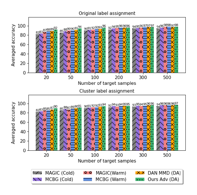
Figure 8: Averaged accuracy on the target testing data for different techniques. The top figure shows the result for the original label of MalwareBazaar and the bottom figure shows the result for the cluster label of MalwareBazaar.

-C More details on the content-based features

• Symbol. The frequencies of symbols -, +, *, ], [, ?, and @ are counted due to their common occurrence in code designed to evade detection.

• Opcode. We have chosen a subset of 93 opcodes from the x86 instruction set, selected for their common usage and their frequent appearance in malicious code. We then measure the frequency of these opcodes in each malware sample.

• Register. The utilization frequency of registers has proven valuable in classifying malware families. Consequently, we have integrated 26 register features into the feature set for this purpose.

• Windows API. We also measure the frequency of use of Windows API in the assembly code. We have selected top 794 frequent APIs used by malicious binaries based on the study in [2].

• Section. A PE file typically comprises predefined sections such as .text, .data, .bss, .rdata, .edata, .idata, .rsrc, .tls, and .reloc. Due to packing, these default sections can be altered, rearranged, and new sections may be introduced. Consequently, the 26 section features are statistical attributes that capture the proportion of each section within the entire assembly file.

• Data Define. Certain malware samples may lack any API calls and primarily consist of a few operation codes, often due to packing. Specifically, they frequently feature data definition instructions like db, dw, and dd. As a result, we have incorporated 18 statistical features that summarize the distinct characteristics of data definition instructions into our analysis.

• Others. We have calculated both the file size and the number of lines within the file.

-D Implementation details on content-based baselines and our approach

-D1 SVM and MLP

For SVM, we set $C=0.1$ to be consistent with [7]. For the MLP, it consists of 8 fully connected layers (FC_1,FC_1,…, FC_OUT), with 100 neurons in FC1-5 and 400 neurons in FC5-6, while FC_OUT serves as the output layer for label prediction. MLP is trained using Adam optimizer with a learning rate of $\mathit{1e-3}$ for 60 epochs. In warm-start of MLP, we continue training all the layers of the older model.

-D2 Our approach

Our model is implemented to be comparable with the MLP. The generator comprises 5 dense layers, each with 100 neurons. The classifier architecture consists of 3 fully connected layers, with the first two layers having 400 neurons each, and the final layer serving as the output layer. Essentially, the combined generator and classifier components form the classifier model described above. The discriminator has four layers with 400 hidden units, followed by the softmax layer for domain prediction. The hyperparameters remain consistent with those outlined in Appendix -A1.

-D3 DAN

The feature extractor comprises 5 dense layers, each with 100 neurons. The classifier architecture consists of 3 fully connected layers, with the first two layers having 400 neurons each, and the final layer serving as the output layer. The hyperparameters remain consistent with those outlined in Appendix -A2.

-E Implementation details on image-based baselines

-E1 Our approach

The generator has the architecture of (Conv2D, MaxPooling, Conv2D, MaxPooling, Flatten). The Conv2D layers has $\{32,64\}$ $3\times 3$ filters respectively. The classifier consists of 2 fully connected layers (FC_1, FC_OUT). The number of neurons in FC1 is 256. FC_OUT is the output layers for label prediction. The discriminator has two layers with 1024 hidden units and is followed by the softmax layer for domain prediction. Batch normalization is applied on every hidden layer. For training the model, we use the Adam optimizer with a learning rate of $\mathit{1e-3}$ for 60 epochs. The batch size is 32. The coefficient of the loss $\mathcal{L}_{g}$ is set to 0.1. We set $\lambda=0.1$ in $\mathcal{L}_{c}$.

-E2 ResNet (Cold) and (Warm)

The original ResNet-50’s output layer contains 1000 neurons. As our task focuses on predicting whether a sample is malware or benign software, we modified the model by removing its last layer, adding a global average pooling layer, incorporating a fully connected layer with 256 neurons, and appending an output layer with 2 neurons. For training the model, we use the Adam optimizer with a learning rate of $\mathit{1e-3}$ for 60 epochs.

-E3 DAN

The feature extractor also has the same architecture as the generator and so as the classifier. For training the model, we use the Adam optimizer with a learning rate of $\mathit{1e-3}$ for 60 epochs. The batch size is 32. The coefficient of the MMD loss is set to 1. We set $\lambda=0.1$ in $\mathcal{L}_{c}$.

-E4 Additional results on representation evaluation

The F1-score can be found in Table XI.

-F Implementation details and additional results on in-class evolution evaluation

The implementation of the baseline models and our approach remain consistent with those outlined in Appendix -A1 and -A2, except for the output layer, which is modified to accommodate 7 classes.

TABLE VII: Evaluation results (F1 score) based on the original label of Big-15.

		Ramnit: target samples						Lollipop: target samples						Kelihos_ver3: target samples
Strategy	Method	20	50	100	200	300	500	20	50	100	200	300	500	20	50	100	200	300	500
	MCBG	79.2	81.4	88.8	89.6	93	98.3	76.8	83.5	85.5	89.2	94	98.3	78.7	85.5	88.6	93	95.3	97
Cold	MAGIC	73.8	80.4	86.9	89.2	90.1	94.5	75.9	83.2	84.7	88.4	93.6	96.1	77.9	85.3	87.1	90.0	94.1	96
	MCBG	87.6	89.7	96.3	96.7	99.8	99.7	89.5	93.5	94.1	95.6	96.9	98.5	89.8	94.9	95.1	96.2	97.1	98.8
Warm	MAGIC	80.0	82.0	92.0	94.7	95.3	98.8	87.7	91.9	93.8	95.4	97.1	98.7	87.7	94.1	94.1	96.4	97.4	98.6
	DAN (MMD)	88.3	92.5	96.5	99.3	99.8	99.7	93.0	93.8	97.4	98.5	99.8	99.8	90.1	94.8	98.5	99.6	99.8	99.9
		91.0	95.6	96.7	99.7	99.9	100.0	94.3	95.3	99.8	99.9	99.9	100.0	97.0	97.4	99.7	99.9	100	100
DA	Ours (Adv)	$\uparrow$2.7	$\uparrow$3.1	$\uparrow$0.2	$\uparrow$0.4	$\uparrow$0.1	$\uparrow$0.3	$\uparrow$1.3	$\uparrow$1.5	$\uparrow$2.4	$\uparrow$1.4	$\uparrow$0.1	$\uparrow$0.2	$\uparrow$6.9	$\uparrow$2.5	$\uparrow$1.2	$\uparrow$0.3	$\uparrow$0.2	$\uparrow$0.1

TABLE VIII: Evaluation results (F1 score) based on the cluster label of Big-15.

		Cluster 0: target samples						Cluster 1: target samples						Cluster 2: target samples
Strategy	Method	20	50	100	200	300	500	20	50	100	200	300	500	20	50	100	200	300	500
	MCBG	79.9	85.9	88.7	89.3	93.0	98.8	79.6	78.9	84.5	87.4	91.5	96.1	76.6	85.7	88.6	91.9	97.9	99.2
Cold	MAGIC	74.6	85.5	87.4	89.6	92.0	96.3	76.5	79.4	82.5	87.2	91.1	93.5	76.9	85.2	88.5	90.9	96.0	98.7
	MCBG	87.5	88.0	91.1	93.8	96.5	99.0	86.1	87.0	88.8	92.5	97.5	99.6	83.0	88.3	90.1	96.2	98.5	99.3
Warm	MAGIC	87.5	87.9	90.3	92.9	95.4	96.4	84.3	84.7	88.0	91.9	92.1	93.5	82.6	87.2	90.2	96.6	98.5	99.0
	DAN (MMD)	92.3	93.5	94.0	94.1	99.4	99.6	89.8	91.1	87.3	99.0	99.5	99.6	88.8	91.2	98.5	99.6	100	100
		93.5	95.0	98.1	96.7	99.5	99.6	93.1	95.8	99.2	99.7	99.5	99.6	91.4	93.5	99.4	99.7	100	100
DA	Ours (Adv)	$\uparrow$1.2	$\uparrow$1.5	$\uparrow$4.1	$\uparrow$2.6	$\uparrow$0.1	$\uparrow$0	$\uparrow$3.3	$\uparrow$4.7	$\uparrow$10.4	$\uparrow$0.7	$\uparrow$0	$\uparrow$0	$\uparrow$2.6	$\uparrow$2.3	$\uparrow$0.9	$\uparrow$0.1	$\uparrow$0	$\uparrow$0

TABLE IX: Evaluation results (accuracy and F1 score) based on the original label of MalwareBazaar.

			Gozi: target samples						Guloader: target samples						Trickbot: target samples
Metric	Strategy	Method	20	50	100	200	300	500	20	50	100	200	300	500	20	50	100	200	300	500
		MCBG	83.7	88.4	92.5	94.7	94.4	96.6	84.7	89.9	92.6	95.2	96.4	97.1	79.8	84.4	87.9	92.3	93.2	94.5
	Cold	MAGIC	82.4	86.1	89.8	91.7	93.1	94.1	83.8	85.4	92.5	93.5	95.4	95.8	78.7	83.4	86.7	90.9	92.2	93.4
		MCBG	87.3	91.0	93.9	95.8	97.1	98.6	90.9	91.6	94.2	97.9	98.4	99.5	86.6	87.7	91.1	94.0	94.5	95.0
	Warm	MAGIC	85.1	90.9	92.3	94.2	95.6	97.6	90.0	91.3	94.1	98.0	98.4	99.2	85.8	88.9	90.6	93.7	94.7	95.7
		DAN (MMD)	90.2	92.7	93.9	94.7	97.0	98.0	91.0	92.8	94.7	98.1	98.4	98.5	87.0	88.8	91.3	93.8	94.0	95.5
			90.3	93.3	94.5	95.8	97.4	98.6	92.0	95.2	98.0	98.1	98.8	99.7	92.7	93.0	94.1	94.4	94.7	95.7
Accuracy	DA	Ours (Adv)	$\uparrow$0.1	$\uparrow$0.6	$\uparrow$1.5	$\uparrow$1.1	$\uparrow$0.3	$\uparrow$0	$\uparrow$1	$\uparrow$2.4	$\uparrow$3.3	$\uparrow$0	$\uparrow$0.4	$\uparrow$1.2	$\uparrow$5.7	$\uparrow$4.1	$\uparrow$2.8	$\uparrow$0.4	$\uparrow$0	$\uparrow$0
		MCBG	83.6	88.1	92.0	94.7	94.4	96.7	84.5	89.5	92.6	95.0	96.1	97.1	78.8	82.4	87.9	92.0	93.2	94.4
	Cold	MAGIC	82.5	86.1	89.8	91.0	93.1	94.1	83.8	85.4	92.6	93.5	95.4	95.8	78.7	83.4	86.5	90.9	92.2	93.4
		MCBG	87.3	91.0	94.0	95.8	97.1	98.6	91.5	91.7	94.3	98.0	98.4	99.5	86.6	87.8	91.2	94.2	94.5	95.0
	Warm	MAGIC	85.2	90.9	92.3	94.1	95.5	97.6	89.9	91.4	94.1	98.5	98.4	99.2	85.7	88.9	90.6	93.7	94.7	95.7
		DAN (MMD)	90.1	92.7	94.0	94.7	97.0	98.0	91.0	92.9	95.0	98.1	98.4	98.5	87.0	88.8	91.3	93.8	94.0	95.5
			90.3	93.3	94.0	95.8	97.4	98.6	92.0	95.2	98.0	98.9	98.9	99.6	92.7	93.0	94.1	94.4	94.7	95.7
F1	DA	Ours (Adv)	$\uparrow$0.2	$\uparrow$0.6	$\uparrow$0	$\uparrow$0	$\uparrow$0.3	$\uparrow$0	$\uparrow$0.5	$\uparrow$2.3	$\uparrow$3	$\uparrow$0.4	$\uparrow$0.5	$\uparrow$0.1	$\uparrow$5.7	$\uparrow$4.1	$\uparrow$2.8	$\uparrow$0.2	$\uparrow$0	$\uparrow$0

TABLE X: Evaluation results (accuracy and F1 score) based on the cluster label of MalwareBazaar.

			Cluster 0: target samples						Cluster 1: target samples						Cluster 2: target samples
Metric	Strategy	Method	20	50	100	200	300	500	20	50	100	200	300	500	20	50	100	200	300	500
		MCBG	80.6	88.9	91.5	94	94.4	95.4	82.7	85	90.1	94.2	96.2	97.1	84.5	89	91.5	93.2	94.2	96.6
	Cold	MAGIC	80.5	85.7	89.9	90.8	92.3	93.1	80.8	82.3	89.9	91.7	92.7	94.7	82.2	86.7	90.4	92.2	94.1	94.5
		MCBG	84.4	90.2	91.7	94.4	94.8	95.3	84.5	86.1	92.3	94.5	96.0	97.0	86.3	90.6	93.2	94.9	95.0	96.5
	Warm	MAGIC	83.6	86.1	91.1	92.7	93.5	94.6	83.8	84.1	90.5	92.4	94.0	95.7	86.7	90.8	93.3	94.1	95.3	96.1
		DAN (MMD)	86.2	90.9	92.0	94.6	95.4	95.3	87.0	87.3	93.3	95.2	96.8	97.1	87.8	92.0	93.9	94.5	95.7	96.0
			89.6	91.7	93.5	95.4	96.0	96.0	88.4	89.1	93.5	95.5	96.8	97.0	90.4	92.7	93.9	94.9	95.6	96.5
Accuracy	DA	Ours (Adv)	$\uparrow$3.4	$\uparrow$0.8	$\uparrow$1.5	$\uparrow$0.8	$\uparrow$0.6	$\uparrow$0.7	$\uparrow$1.4	$\uparrow$1.8	$\uparrow$0.2	$\uparrow$0.3	$\uparrow$0	$\downarrow$0.1	$\uparrow$2.6	$\uparrow$0.7	$\uparrow$0	$\uparrow$0	$\downarrow$-0.1	$\uparrow$0
		MCBG	80.8	88.9	91.5	94.0	94.4	95.4	82.7	85.3	90.3	94.3	96.3	97.1	84.5	89.0	91.2	93.2	94.2	96.6
	Cold	MAGIC	80.5	85.7	90.0	90.6	92.7	93.1	79.5	81.8	89.3	91.7	92.8	94.7	82.2	86.8	90.4	92.2	94.1	94.2
		MCBG	84.3	90.0	91.5	94.4	94.8	95.3	84.8	86.3	92.4	94.5	96.1	97.0	86.8	90.6	93.2	94.9	95.0	96.5
	Warm	MAGIC	83.6	86.1	91.2	92.8	93.4	94.6	84.1	84.3	90.7	92.3	94.1	95.8	86.7	90.8	93.3	94.1	95.3	96.1
		DAN (MMD)	86.2	90.9	92.0	94.6	95.4	95.3	87.0	87.3	93.3	95.0	96.8	97.1	87.8	92.0	93.9	94.5	95.7	96.0
			89.6	91.7	93.5	95.4	95.9	96.0	88.0	89.2	93.5	95.5	96.8	97.0	90.1	92.7	93.9	94.9	95.6	96.6
F1	DA	Ours (Adv)	$\uparrow$3.4	$\uparrow$0.8	$\uparrow$1.5	$\uparrow$0.8	$\uparrow$0.5	$\uparrow$0.7	$\uparrow$1	$\uparrow$1.9	$\uparrow$0.2	$\uparrow$0.5	$\uparrow$0	$\downarrow$0.1	$\uparrow$2.3	$\uparrow$0.7	$\uparrow$0	$\uparrow$0	$\downarrow$-0.1	$\uparrow$0

TABLE XI: F1 of baselines across various malware representations. In terms of content and image representation, we illustrate the percentage change in accuracy from our adversarial (Adv) DA method to the peak performance among all baselines within the same representation. Ultimately, we demonstrate the enhancements of our full pipeline (graph + Adv DA) compared to both content + Adv DA and image + Adv DA.

			Cluster 0: target samples						Cluster 1: target samples						Cluster 2: target samples
Malware Representation	Strategy	Method	20	50	100	200	300	500	20	50	100	200	300	500	20	50	100	200	300	500
		SVM	79.1	83.3	84.2	88.8	90.5	93.0	73.5	75.6	76.5	84.7	88.9	90.2	80.0	86.2	88.1	90.3	96.2	97.5
	Cold	MLP	82.4	85.1	90.2	91.6	94.3	96.4	73.7	79.3	82.4	89.9	90.8	95.7	80.5	86.7	88.1	91.8	96.6	97.3
		SVM	82.4	83.5	89.6	91.0	91.8	93.5	75.5	77.4	79.8	86.1	89.0	90.2	81.1	85.2	88.9	95.4	98.0	99.2
	Warm	MLP	84.2	88.1	91.1	93.6	95.7	96.9	82.1	87.5	86.3	92.0	93.7	95.6	80.0	84.9	89.5	96.6	98.6	99.2
		DAN (MMD) + MLP	83.3	89.4	91.2	93.5	94.8	97.0	83.0	87.0	89.2	93.0	94.0	95.1	80.5	85.7	89.3	96.5	98.0	99.0
			87.3	90.2	93.5	94.0	95.7	96.9	85.0	89.8	90.9	93.6	95.0	95.9	83.6	87.4	90.7	96.4	98.5	99.0
Content-based (CB)	DA	Ours (Adv) + MLP	$\uparrow$3.1	$\uparrow$0.8	$\uparrow$2.3	$\uparrow$0.4	$\uparrow$0	$\downarrow$0.1	$\uparrow$2.0	$\uparrow$2.3	$\uparrow$1.7	$\uparrow$0.6	$\uparrow$1.0	$\uparrow$0.2	$\uparrow$2.5	$\uparrow$0.7	$\uparrow$1.0	$\downarrow$0.2	$\downarrow$0.1	$\downarrow$0.2
	Cold	ResNet-50	50.3	50.3	75.5	88.0	90.8	92.1	49.9	54.3	65.3	76.9	88.0	91.3	49.5	61.3	67.6	72.5	82.0	87.0
	Warm	ResNet-50	88.3	90.9	91.8	93.6	94.9	96.6	80.3	86.4	88.0	89.7	92.3	93.8	81.8	83.6	88.5	90.4	90.6	94.7
		DAN (MMD) + CNN	89.4	90.2	91.7	93.3	94.0	96.3	86.0	89.5	90.8	92.5	94.2	94.5	85.2	86.2	89.8	90.5	91.5	94.4
			89.6	92.5	94.0	94.9	95.0	96.7	90.8	92.1	93.2	94.3	94.5	95.4	86.5	87.2	90.3	91.3	93.9	94.4
Image-based (IB)	DA	Ours (Adv) + CNN	$\uparrow$0.2	$\uparrow$1.6	$\uparrow$2.2	$\uparrow$1.3	$\uparrow$0.1	$\uparrow$0.1	$\uparrow$4.8	$\uparrow$2.6	$\uparrow$2.2	$\uparrow$2.4	$\uparrow$0.3	$\uparrow$0.9	$\uparrow$1.3	$\uparrow$1	$\uparrow$0.5	$\uparrow$0.8	$\uparrow$2.4	$\downarrow$0.3
Graph-based (GB)	DA	Ours (Adv) + GIN	93.5	95.0	98.1	96.7	99.5	99.6	93.1	95.8	99.2	99.7	99.5	99.6	91.4	93.5	99.4	99.7	100	100
Improvement over CB			$\uparrow$6.2	$\uparrow$4.8	$\uparrow$4.6	$\uparrow$2.7	$\uparrow$3.8	$\uparrow$2.7	$\uparrow$8.1	$\uparrow$6	$\uparrow$8.3	$\uparrow$6.1	$\uparrow$4.5	$\uparrow$3.7	$\uparrow$7.8	$\uparrow$6.1	$\uparrow$8.7	$\uparrow$3.3	$\uparrow$1.5	$\uparrow$1
Improvement over IB			$\uparrow$3.9	$\uparrow$2.5	$\uparrow$4.1	$\uparrow$1.8	$\uparrow$4.5	$\uparrow$2.9	$\uparrow$2.3	$\uparrow$3.7	$\uparrow$6	$\uparrow$5.4	$\uparrow$5	$\uparrow$4.2	$\uparrow$4.9	$\uparrow$6.3	$\uparrow$9.1	$\uparrow$8.4	$\uparrow$6.1	$\uparrow$5.6

TABLE XII: Accuracy and F1 score on post-drift testing data using a few labeled data from each family in post-drift training data.

			Target samples per family
Metric	Strategy	Method	10	20	30	40	45
		MCBG	21.3	34.6	39.3	62.8	72.4
	Cold	MAGIC	20.8	33.0	39.1	58.7	68.6
		MCBG	70.7	77.2	82.2	85.3	87.1
	Warm	MAGIC	69.0	74.7	81.9	82.0	83.1
		DAN (MMD) + GIN	74.4	84.4	85.6	88.0	89.6
			82.3	87.5	88.4	90.0	90.6
Accuracy	DA	Ours (Adv) + GIN	$\uparrow$7.9	$\uparrow$3.1	$\uparrow$2.8	$\uparrow$2	$\uparrow$1
		MCBG	24.6	30.7	39.7	63.6	73.2
	Cold	MAGIC	22.0	30.4	39.5	56.0	67.5
		MCBG	71.5	77.6	81.8	84.9	87.9
	Warm	MAGIC	69.0	74.7	79.1	80.7	84.0
		DAN (MMD) + GIN	75.4	84.5	85.6	88.0	89.6
			81.6	87.3	88.0	89.0	89.7
F1	DA	Ours (Adv) + GIN	$\uparrow$6.2	$\uparrow$2.8	$\uparrow$2.4	$\uparrow$1	$\uparrow$0.1

References

- [1] H. Aghakhani, F. Gritti, F. Mecca, M. Lindorfer, S. Ortolani, D. Balzarotti, G. Vigna, and C. Kruegel, “When malware is packin’heat; limits of machine learning classifiers based on static analysis features,” in Network and Distributed Systems Security (NDSS) Symposium 2020, 2020.
- [2] M. Ahmadi, D. Ulyanov, S. Semenov, M. Trofimov, and G. Giacinto, “Novel feature extraction, selection and fusion for effective malware family classification,” in Proceedings of the sixth ACM conference on data and application security and privacy, 2016, pp. 183–194.
- [3] F. Barbero, F. Pendlebury, F. Pierazzi, and L. Cavallaro, “Transcending transcend: Revisiting malware classification in the presence of concept drift,” in 2022 IEEE Symposium on Security and Privacy (SP). IEEE, 2022, pp. 805–823.
- [4] S. Bhardwaj, A. S. Li, M. Dave, and E. Bertino, “Overcoming the lack of labeled data: Training malware detection models using adversarial domain adaptation,” Computers & Security, p. 103769, 2024.
- [5] N. Bhodia, P. Prajapati, F. Di Troia, and M. Stamp, “Transfer learning for image-based malware classification,” arXiv preprint arXiv:1903.11551, 2019.
- [6] T. Caliński and J. Harabasz, “A dendrite method for cluster analysis,” Communications in Statistics-theory and Methods, vol. 3, no. 1, pp. 1–27, 1974.
- [7] Y. Chen, Z. Ding, and D. Wagner, “Continuous learning for android malware detection,” in 32nd USENIX Security Symposium (USENIX Security 23), 2023, pp. 1127–1144.
- [8] Q. Dai, X.-M. Wu, J. Xiao, X. Shen, and D. Wang, “Graph transfer learning via adversarial domain adaptation with graph convolution,” IEEE Transactions on Knowledge and Data Engineering, vol. 35, no. 5, pp. 4908–4922, 2022.
- [9] S. Dambra, Y. Han, S. Aonzo, P. Kotzias, A. Vitale, J. Caballero, D. Balzarotti, and L. Bilge, “Decoding the secrets of machine learning in malware classification: A deep dive into datasets, feature extraction, and model performance,” in Proceedings of the 2023 ACM SIGSAC Conference on Computer and Communications Security, 2023, pp. 60–74.
- [10] D. L. Davies and D. W. Bouldin, “A cluster separation measure,” IEEE transactions on pattern analysis and machine intelligence, no. 2, pp. 224–227, 1979.
- [11] Y. Ganin, E. Ustinova, H. Ajakan, P. Germain, H. Larochelle, F. Laviolette, M. Marchand, and V. Lempitsky, “Domain-adversarial training of neural networks,” The journal of machine learning research, vol. 17, no. 1, pp. 2096–2030, 2016.
- [12] I. Goodfellow, J. Pouget-Abadie, M. Mirza, B. Xu, D. Warde-Farley, S. Ozair, A. Courville, and Y. Bengio, “Generative adversarial networks,” Communications of the ACM, vol. 63, no. 11, pp. 139–144, 2020.
- [13] D. Han, Z. Wang, W. Chen, K. Wang, R. Yu, S. Wang, H. Zhang, Z. Wang, M. Jin, J. Yang et al., “Anomaly detection in the open world: Normality shift detection, explanation, and adaptation.” in NDSS, 2023.
- [14] K. He, X. Zhang, S. Ren, and J. Sun, “Deep residual learning for image recognition,” in Proceedings of the IEEE conference on computer vision and pattern recognition, 2016, pp. 770–778.
- [15] Y. Hou, T. Truong-Huu, Z. Chen, C.-K. Kwoh, and S. G. Teo, “Proteus: Domain adaptation for dynamic features in ai-assisted windows malware detection,” in 2023 IEEE International Conference on Data Mining Workshops (ICDMW). IEEE, 2023, pp. 1322–1331.
- [16] R. Jordaney, K. Sharad, S. K. Dash, Z. Wang, D. Papini, I. Nouretdinov, and L. Cavallaro, “Transcend: Detecting concept drift in malware classification models,” in 26th USENIX security symposium (USENIX security 17), 2017, pp. 625–642.
- [17] Z. Kan, F. Pendlebury, F. Pierazzi, and L. Cavallaro, “Investigating labelless drift adaptation for malware detection,” in Proceedings of the 14th ACM Workshop on Artificial Intelligence and Security, 2021, pp. 123–134.
- [18] T. N. Kipf and M. Welling, “Variational graph auto-encoders,” arXiv preprint arXiv:1611.07308, 2016.
- [19] S. Kumar et al., “Mcft-cnn: Malware classification with fine-tune convolution neural networks using traditional and transfer learning in internet of things,” Future Generation Computer Systems, vol. 125, pp. 334–351, 2021.
- [20] A. S. Li, E. Bertino, X.-H. Dang, A. Singla, Y. Tu, and M. N. Wegman, “Maximal domain independent representations improve transfer learning,” arXiv preprint arXiv:2306.00262, 2023.
- [21] A. S. Li, A. Iyengar, A. Kundu, and E. Bertino, “Transfer learning for security: Challenges and future directions,” arXiv preprint arXiv:2403.00935, 2024.
- [22] H. Li, Z. Chen, R. Spolaor, Q. Yan, C. Zhao, and B. Yang, “Dart: Detecting unseen malware variants using adaptation regularization transfer learning,” in ICC 2019-2019 IEEE International Conference on Communications (ICC). IEEE, 2019, pp. 1–6.
- [23] X. Li, Y. Xin, H. Zhu, Y. Yang, and Y. Chen, “Cross-domain vulnerability detection using graph embedding and domain adaptation,” Computers & Security, vol. 125, p. 103017, 2023.
- [24] X. Li, Y. Qu, and H. Yin, “Palmtree: Learning an assembly language model for instruction embedding,” in Proceedings of the 2021 ACM SIGSAC Conference on Computer and Communications Security, 2021, pp. 3236–3251.
- [25] M. Long, Y. Cao, J. Wang, and M. Jordan, “Learning transferable features with deep adaptation networks,” in International conference on machine learning. PMLR, 2015, pp. 97–105.
- [26] Y. Ma, S. Liu, J. Jiang, G. Chen, and K. Li, “A comprehensive study on learning-based pe malware family classification methods,” in Proceedings of the 29th ACM Joint Meeting on European Software Engineering Conference and Symposium on the Foundations of Software Engineering, 2021, pp. 1314–1325.
- [27] E. Mariconti, L. Onwuzurike, P. Andriotis, E. De Cristofaro, G. Ross, and G. Stringhini, “Mamadroid: Detecting android malware by building markov chains of behavioral models,” arXiv preprint arXiv:1612.04433, 2016.
- [28] L. Massarelli, G. A. Di Luna, F. Petroni, L. Querzoni, R. Baldoni et al., “Investigating graph embedding neural networks with unsupervised features extraction for binary analysis,” in Proceedings of the 2nd Workshop on Binary Analysis Research (BAR), 2019, pp. 1–11.
- [29] A. Narayanan, M. Chandramohan, L. Chen, and Y. Liu, “Context-aware, adaptive, and scalable android malware detection through online learning,” IEEE Transactions on Emerging Topics in Computational Intelligence, vol. 1, no. 3, pp. 157–175, 2017.
- [30] A. Narayanan, L. Yang, L. Chen, and L. Jinliang, “Adaptive and scalable android malware detection through online learning,” in 2016 International Joint Conference on Neural Networks (IJCNN). IEEE, 2016, pp. 2484–2491.
- [31] L. Nataraj, S. Karthikeyan, G. Jacob, and B. S. Manjunath, “Malware images: visualization and automatic classification,” in Proceedings of the 8th international symposium on visualization for cyber security, 2011, pp. 1–7.
- [32] Y. M. Pa Pa, S. Tanizaki, T. Kou, M. Van Eeten, K. Yoshioka, and T. Matsumoto, “An attacker’s dream? exploring the capabilities of chatgpt for developing malware,” in Proceedings of the 16th Cyber Security Experimentation and Test Workshop, 2023, pp. 10–18.
- [33] F. Pendlebury, F. Pierazzi, R. Jordaney, J. Kinder, and L. Cavallaro, “TESSERACT: Eliminating experimental bias in malware classification across space and time,” in 28th USENIX security symposium (USENIX Security 19), 2019, pp. 729–746.
- [34] R. Ronen, M. Radu, C. Feuerstein, E. Yom-Tov, and M. Ahmadi, “Microsoft malware classification challenge,” arXiv preprint arXiv:1802.10135, 2018.
- [35] P. J. Rousseeuw, “Silhouettes: a graphical aid to the interpretation and validation of cluster analysis,” Journal of computational and applied mathematics, vol. 20, pp. 53–65, 1987.
- [36] G. Salha, R. Hennequin, and M. Vazirgiannis, “Keep it simple: Graph autoencoders without graph convolutional networks,” arXiv preprint arXiv:1910.00942, 2019.
- [37] X. Shen, Q. Dai, S. Mao, F.-l. Chung, and K.-S. Choi, “Network together: Node classification via cross-network deep network embedding,” IEEE Transactions on Neural Networks and Learning Systems, vol. 32, no. 5, pp. 1935–1948, 2020.
- [38] A. Singh, A. Handa, N. Kumar, and S. K. Shukla, “Malware classification using image representation,” in Cyber Security Cryptography and Machine Learning: Third International Symposium, CSCML 2019, Beer-Sheva, Israel, June 27–28, 2019, Proceedings 3. Springer, 2019, pp. 75–92.
- [39] A. Singla, E. Bertino, and D. Verma, “Preparing network intrusion detection deep learning models with minimal data using adversarial domain adaptation,” in Proceedings of the 15th ACM Asia conference on computer and communications security, 2020, pp. 127–140.
- [40] M. Someya, Y. Otsubo, and A. Otsuka, “Fcgat: Interpretable malware classification method using function call graph and attention mechanism,” in Proceedings of Network and Distributed Systems Security (NDSS) Symposium, vol. 1, 2023.
- [41] E. Tzeng, J. Hoffman, K. Saenko, and T. Darrell, “Adversarial discriminative domain adaptation,” in Proceedings of the IEEE conference on computer vision and pattern recognition, 2017, pp. 7167–7176.
- [42] D. Vasan, M. Alazab, S. Wassan, H. Naeem, B. Safaei, and Q. Zheng, “Imcfn: Image-based malware classification using fine-tuned convolutional neural network architecture,” Computer Networks, vol. 171, p. 107138, 2020.
- [43] M. Wadkar, F. Di Troia, and M. Stamp, “Detecting malware evolution using support vector machines,” Expert Systems with Applications, vol. 143, p. 113022, 2020.
- [44] F. Wang, G. Chai, Q. Li, and C. Wang, “An efficient deep unsupervised domain adaptation for unknown malware detection,” Symmetry, vol. 14, no. 2, p. 296, 2022.
- [45] H. Wang, W. Qu, G. Katz, W. Zhu, Z. Gao, H. Qiu, J. Zhuge, and C. Zhang, “Jtrans: Jump-aware transformer for binary code similarity detection,” in Proceedings of the 31st ACM SIGSOFT International Symposium on Software Testing and Analysis, 2022, pp. 1–13.
- [46] B. Wu, Y. Xu, and F. Zou, “Malware classification by learning semantic and structural features of control flow graphs,” in 2021 IEEE 20th International Conference on Trust, Security and Privacy in Computing and Communications (TrustCom). IEEE, 2021, pp. 540–547.
- [47] Y. Xie, J. Yi, J. Shao, J. Curl, L. Lyu, Q. Chen, X. Xie, and F. Wu, “Defending chatgpt against jailbreak attack via self-reminders,” Nature Machine Intelligence, vol. 5, no. 12, pp. 1486–1496, 2023.
- [48] K. Xu, Y. Li, R. Deng, K. Chen, and J. Xu, “Droidevolver: Self-evolving android malware detection system,” in 2019 IEEE European Symposium on Security and Privacy (EuroS&P). IEEE, 2019, pp. 47–62.
- [49] K. Xu, W. Hu, J. Leskovec, and S. Jegelka, “How powerful are graph neural networks?” arXiv preprint arXiv:1810.00826, 2018.
- [50] J. Yan, G. Yan, and D. Jin, “Classifying malware represented as control flow graphs using deep graph convolutional neural network,” in 2019 49th annual IEEE/IFIP international conference on dependable systems and networks (DSN). IEEE, 2019, pp. 52–63.
- [51] L. Yang, W. Guo, Q. Hao, A. Ciptadi, A. Ahmadzadeh, X. Xing, and G. Wang, “CADE: Detecting and explaining concept drift samples for security applications,” in 30th USENIX Security Symposium (USENIX Security 21), 2021, pp. 2327–2344.
- [52] H. Yin, B. Lou, and P. Reiher, “A method for summarizing and classifying evasive malware,” in Proceedings of the 26th International Symposium on Research in Attacks, Intrusions and Defenses, 2023, pp. 455–470.
- [53] A. Zewe, “Avoiding shortcut solutions in artificial intelligence,” https://news.mit.edu/2021/shortcut-artificial-intelligence-1102, 2021, [Online; accessed April 2024].
- [54] C. Zhang, B. Liu, Y. Xin, and L. Yao, “Cpvd: Cross project vulnerability detection based on graph attention network and domain adaptation,” IEEE Transactions on Software Engineering, 2023.