Efficient and Device-Independent Active Quantum State Certification

Abstract

Entangled quantum states are essential ingredients for many quantum technologies, but they must be validated before they are used. As a full characterization is prohibitively resource-intensive, recent work has focused on developing methods to efficiently extract a few parameters of interest, in a so-called verification framework. Most existing approaches are based on preparing an ensemble of nominally identical and independent (IID) quantum states, and then measuring each copy of the ensemble. However, this leaves no states left for the intended quantum tasks and the IID assumptions do not always hold experimentally. To overcome these challenges, we experimentally implement quantum state certification (QSC), which measures only a subset of the ensemble, certifying the fidelity of the remaining states. We use active optical switches to randomly sample from sources of two-photon Bell states and three-photon GHZ states, reporting statistically-sound fidelities in real time without destroying the entire ensemble. Additionally, our QSC protocol removes the assumption that the states are identical, is device-independent, and can achieve close $N^{-1}$ scaling, in the number of states measured $N$. Altogether, these benefits make our QSC protocol suitable for benchmarking large-scale quantum computing devices and deployed quantum communication setups relying on entanglement in both standard and adversarial situations.

Quantum technology uses entangled states as resources to implement tasks with an efficiency or security that cannot be accomplished with only classical resources [1, 2]. However, before using an entangled state for a given task the experimentally produced state must be verified. Traditionally, this is done by preparing an ensemble of $N$ identical and independently distributed (IID) states and measuring each state. It is widely appreciated that learning the complete quantum state—i.e. performing quantum state tomography [3]—is a challenging task, requiring $N$ to increase exponentially with the system size. This has led to a variety of resource efficient characterization methods, including adaptive state tomography [4, 5, 6], compressed sensing [7], direct fidelity estimation [8], cross-verification [9, 10] and quantum state verification (QSV) [11, 12, 13, 14, 15, 16, 17, 18, 19, 20]. In all of these approaches one measures every copy of the initially prepared ensemble, leaving no states for use in a further experiment. One must therefore assume that the source operates identically during the characterization and operation phases. Here, we circumvent this problem by experimentally implementing a recently-proposed quantum state certification (QSC) protocol [21].

In QSC only a subset of the ensemble is measured, allowing one to certify some property of the remaining states. In more detail, we imagine a “verifier” who randomly extracts a subset of the initial ensemble of physical states and a “user” who receives the remaining states. The verifier performs QSV on their sub-ensemble, allowing her to issue a certificate to the user that his remaining states are close to a promised target state. More precisely, QSC considers a set of $N$ independent (but not necessarily identical) physical states. The verifier then extracts a random subset of $\mu N$ states, measuring each one. QSC then answers the question “With what confidence can we conclude that the remaining subset of $(1-\mu)N$ physical states have an average fidelity of at least $95\%$ with the target state?”

Importantly, QSC is experimentally accessible, meaning that all measurements can be made locally and the post-processing complexity is low. This is because it is based on QSV which can estimate the fidelity with the optimal $N^{-1}$ scaling [22, 23]. While much work on state characterization operates in a trusted, device dependent scenario, there is a growing need to perform device-independent (DI) state characterization with untrusted measurement devices [24, 25, 26], for applications such as blind quantum computing [16, 17, 27] and quantum cryptography [28, 29]. Our work is based on the proposal Ref. [21], which introduces DI-QSV and QSC, allowing us to experimentally realize efficient device-independent quantum state certification (DI-QSC).

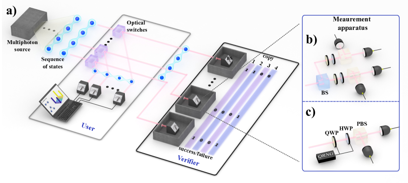
Figure 1: Experimental Quantum State Certification. a) Sequences of $M$-photon states are spontaneously produced and sent to $M$ trusted synchronized optical switches. The switches periodically alternate between two settings, directing the inputs to the user or verifier. We drive the switches faster than the photons are produced. Since the emission time is random, this serves to randomly send each state to the user or verifier. Both the user and verifier implement standard polarization measurements on their photons. b) Two-photon quantum state verification (QSV) measurement. We randomly select the measurement basis for our two-photon experiment using 50:50 beamsplitters to send each of the $M$ photons to one of two polarization measurements. c) Three-photon QSV measurement. For our three-photon experiment, since the three-photon rate is sufficiently low, we randomly select the measurement basis by rotating the waveplates between two settings. Each subsequent setting is chosen based on the outcome of a commercial quantum random number generator (QRNG).

Photonic Bell states and GHZ states are of extreme importance for a variety of applications. In particular, two-photon Bell states are an essential primitive for many quantum communication protocols [30, 29, 31], while three-photon GHZ states can enable the efficient generation of large-scale cluster states for measurement-based quantum computing [32, 33, 34]. Certifying such resources is essential for these and other applications. To show the applicability of our DI-QSC protocol, we therefore experimentally implement it for both two-photon Bell states and three-photon GHZ states [35, 36]. In our implementation of QSC, some of the produced quantum states are randomly routed to the verifier who performs DI-QSV while the user simultaneously runs his experiment. The user can either adapt to the current confidence level broadcasted by the verifier or wait until sufficient confidence is achieved. To realize this deterministically, we use active optical switches [37], as outlined in Fig. 1. If the verifier’s measurements are successful, the remaining states are certified for the user. As we use active switches, each individual state is deterministically routed to the user or verifier. This provides a realistic and practical implementation of QSC, since, from the user’s point of view the only effect is a constant reduction in the counting rate, which does not scale with the system size.

Device Independent Quantum State Certification

Our implementation of DI-QSC is based on self-testing [21]. While the specifics depend on the target state, the idea of selft testing is that certain quantum correlations are almost unique to some target states. For example, self-testing for a GHZ state works as follows. We attempt to violate a Mermin inequality [38] with the physical states. This can only achieved if the physical states are close to the target state. Then, if the violation is sufficiently strong, one can place bounds on the average fidelity $\bar{F}$ of the physical states. We mention that in a DI framework it is not possible to directly assess the fidelity. Instead, one uses the extractability $\Xi$, which is equivalent to the fidelity up to local isometries [39, 40, 41]. However, for simplicity, in the following, we use fidelity $F$ (or infidelity $\eta=1-F$) in place of the extractability if not otherwise specified. Since self-testing is based on estimated probabilities it usually does not discuss the scaling behaviour for finite $N$. [42, 40]. To work in this regime, DI-QSV converts self-testing to a non-local game that can only be won by the target state [21].

To explain DI-QSV, consider a source producing an independent sequence of N states $S=\left\{\sigma_{1},\sigma_{2},...,\sigma_{N}\right\}$, and a target state $|\psi\rangle$ that for now we take to be a three-photon GHZ state. The Mermin inequality for this target state is [38]:

$$B=\sum\limits_{o_{1},o_{2},o_{3}}(-1)^{o_{1}+o_{2}+o_{3}}\left[p(o_{1},o_{2},o_{3}|0,0,1)+p(o_{1},o_{2},o_{3}|0,1,0)+p(o_{1},o_{2},o_{3}|1,0,0)-p(o_{1},o_{2},o_{3}|1,1,1)\right]\leq 2.$$ (1)

Here the individual terms are probabilities of outcomes to be estimated experimentally. In more detail, $p(o_{1},o_{2},o_{3}|i_{1},i_{2},i_{3})$ are the probabilities to obtain outcomes $o_{1}$, $o_{2}$ and $o_{3}$ when qubits one, two and three are measured with a setting defined by $i_{1}$, $i_{2}$ and $i_{3}$. The outputs $o_{i}$ are assumed to be binary, taking values zero or one, which leads to the separable state bounds $B\leq 2$. For an ideal GHZ state, however, the quantum bound is $B_{q}=4$. For the Mermin inequality (Eq.1), there are four measurement settings: $\{i_{1},i_{2},i_{3}\}=\{0,0,1;\leavevmode\nobreak\ 0,1,0;\leavevmode\nobreak\ 1,0,0;\leavevmode\nobreak\ 1,1,1\}$ (defined in the Appendix Eq. 3) each with eight possible outcomes. For a perfect GHZ state only a subset of outcomes will occur with certainty: we group these together, forming the winning outcomes. To make the inequality into a non-local game, we then randomly measure each state of $S$ in one of the four settings, record the number of winning events $n_{\mathrm{wins}}$, and compute the experimental winning probability as $P_{\mathrm{exp}}={n_{\mathrm{wins}}}/{N}$. The intuition is then that since only states equivalent to the target state can violate the inequality, only they can obtain a $P_{exp}$ close to $1$.

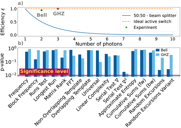
Figure 2: Random Sampling Characterization. (a) Switching efficiency. The blue curve plots the maximum switching efficiency using probabilistic routing with 50:50 beam splitters versus the number of photons in the state to be certified. The dashed line at $1$ indicates the maximum efficiency attainable with the deterministic switches that we use. Our observed two- and three-photon efficiencies of $\epsilon_{2}=0.9439\pm 0.0041$, and $\epsilon_{3}=0.9997\pm 0.0066$, respectively, are plotted as stars. (b) The results of NIST’s statistical test suite for random number generators applied to our sampling of the produced state for two-photon Bell states in dark blue, and three-photon GHZ states in light blue. In both cases, the results exceed the significance threshold of $0.01$, indicating that our implemented sampling is consistent with truly random sampling.

In QSC, the verifier measures $N_{\mathrm{ver}}=\mu N$ states of the initial $N$ state ensemble, and uses her measurement results to estimate $P_{\mathrm{exp}}$. To formalize the relation between $P_{\mathrm{exp}}$ and $\bar{\Xi}$ the average extractability, consider a sequence of $\mu N$ physical states with a reduced average extractability $\bar{\Xi}\leq 1-\eta$. In this case, the maximum winning probability is $P_{\mathrm{\eta}}=P_{\mathrm{QM}}-c\eta$, where $c$ is a constant depending on the specific Bell inequality [21], and $P_{\mathrm{QM}}$ is quantum mechanical probability to win the game (which is $1$ for our present example). If we then observe $P_{\mathrm{exp}}>P_{\mathrm{\eta}}$, the physical states likely have an extractablity $\bar{\Xi}>1-\eta$. However, if $P_{\mathrm{exp}}$ is close to $P_{\mathrm{\eta}}$ it is possible that finite statistical fluctuations led to an ‘accidental’ win. Thus we need to know how likely it is that our observation, $P_{\mathrm{exp}}>P_{\mathrm{\eta}}$, could be reproduced by a series of states with a fidelity less than $F=1-\eta$. This is a classical statistical problem [43, 44]. It can be shown that the probability for a false win after $\mu N$ states are measured is bounded by $\delta\leq e^{-D(P_{\mathrm{exp}}\parallel P_{\mathrm{\eta}})\mu N}$, where $D(x\parallel y)=x\mathrm{log}(x/y)+(1-x)\mathrm{log}\left[(1-x)/(1-y)\right]$ is the Kullback-Leibler divergence [43]. Based on this, Ref. [21] proves that our confidence $C$ that remaining $(1-\mu)N$ states have an average fidelity is greater than $1-\eta$ is

$$C\geq 1-\delta=1-e^{-D(P_{\mathrm{exp}}\parallel P_{\mathrm{\eta}})\mu N},$$ (2)

which grows to $1$ exponentially fast with $N$. See the Supplemental Material Sec. G for more details.

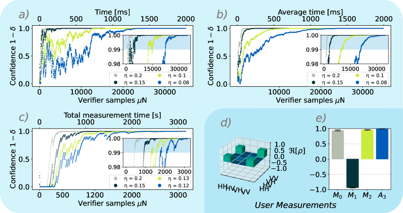
Figure 3: Confidence in two- and three-photon quantum state certification. (a) Confidence versus number of verifier measurements (bottom axis) and measurement time (top axis). The same data set is analyzed for different fidelity $F=1-\eta$ lower bounds. Less stringent bounds (higher values of $\eta$) converge to confidence of $1$ more quickly. The inset shows the high-confidence region, with the shaded area representing a confidence above $0.99$. (b) The two-photon measurement presented in (a) is repeated $12$ times and averaged. The data are plotted as in panel (a). (c) Verifier’s confidence growth for our three-photon GHZ states, plotted as in panel (a). (d) Real part of the density matrix of our two-photon states measured with standard quantum state tomography, taken by the user concurrently with the verifier’s measurements. The plotted density matrix has a fidelity of $0.9947\pm 0.0002$ with the target $|\phi^{+}\rangle$ Bell state. (e) The results of the user’s GHZ witness measurement on our three-photon states, yielding a fidelity of $0.9678\pm 0.0055$ with the target GHZ state. The labels on the x-axis refer to specific measurement settings, defined in the Supplementary Material.

The scaling of the confidence that our physical states have an extractability larger than $1-\eta$ depends on the statistical distance between $P_{\mathrm{exp}}$ and $P_{\mathrm{\eta}}$ (eq. 2). The estimated number of measured states needed to verify this lower bound is $N\geq\frac{\mathrm{ln}\ \delta}{\mathrm{ln}(1-\mu+\mu e^{D(P_{\mathrm{exp}}\parallel P_{\mathrm{\eta}})})}$ [21]. Experimentally, instead, we often wish to compute the fidelity from the results from a set of measurement results. We can also use DI-QSC for this. It results in two different scaling behaviours related to the specifics of the Bell inequality used to make the non-local game. In particular, not all states have Bell inequalities that achieve a perfect success probability when translated to a non-local game. This happens when quantum mechanics cannot achieve the maximum algebraic bound of the Bell inequality. For example, for the CHSH inequality the quantum Tirelson bound $B_{q}=2\sqrt{2}$ is less than the algebraic bound of $4$. When this occurs, we also need to consider the ideal winning probability $P_{\mathrm{QM}}$. These scenarios arise when some winning outcomes do not occur $100\%$ of time. We can still define the set of winning outcomes, but now they are given by the most likely outcomes. When $p_{QM}<1$, the verifiable infidelity scales as $\eta\propto O(\frac{\sqrt{\mathrm{ln}\ \delta^{-1}}}{c\mu(1-\mu)\sqrt{N}})$, i.e. with a sub-optimal $N^{-1/2}$ scaling. However, when $p_{QM}=1$ we can obtain the optimal $N^{-1}$ Heisenberg scaling $\eta\propto O(\frac{\mathrm{ln}\ \delta^{-1}}{c\mu(1-\mu)N})$. Note that these scaling behaviours are derived in the limit of large $N$, and, as we will see later, in our intermediate regime, they are only approximate. Nevertheless, as we will show experimentally, this means that for the two-photon Bell state, using the CHSH inequality we expect to achieve approximate $N^{-1/2}$ scaling, but the 3-photon GHZ state with the Mermin inequality can exceed this scaling.

Experimental Apparatus for Quantum State Certification

We will now present our experimental implementation of DI-QSC for bipartite and tripartite states, allowing us to demonstrate both scaling behaviors discussed above. For the two-photon case, we use a type-0 spontaneous parametric down-conversion (SPDC) source in Sagnac configuration [45] to generate the Bell-state $|\Phi^{+}\rangle=\frac{1}{\sqrt{2}}(|HH\rangle_{1,2}+|VV\rangle_{1,2})$, while for the tripartite case, we employ a three-photon Greenberger-Horn-Zeilinger (GHZ) state $|\Psi_{GHZ}\rangle=\frac{1}{\sqrt{2}}(|HHH\rangle_{1,2,3}+|VVV\rangle_{1,2,3})$ produced by two sandwich-like SPDC sources [46]. For a full description of the photon sources, see the Supplementary Material, Sec. A and B. In both scenarios, we assume that the subsequent states emitted by the source are independent.

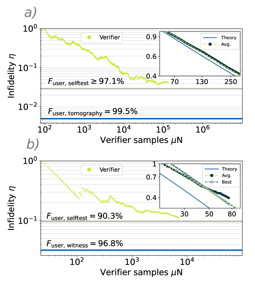
Figure 4: Quantum state certification fidelity scaling at $99\%$ confidence. The estimated infidelities $\eta$ when setting the confidence $C=1-\delta=0.99$ for (a) two-photon Bell states and (b) three-photon GHZ states plotted versus the verifier’s measurement number. In both cases, the infidelity $\eta$ certified by the verifier (green points) asymptotically approaches infidelity estimated by the user with self-testing (grey lines). The user estimates lower infidelities when using device-dependent methods (blue lines) Insets: The insets plot averaged results over smaller sample ranges to estimate the scaling $s$. The dark points are the averaged data, and the dashed green lines are linear fits with slopes of ($s_{\text{Bell, Avg.}}=-0.549$, $s_{\text{GHZ, Avg.}}=-0.801$), respectively. The solid blue line is theory, demonstrating scalings of $s_{\text{Bell, Theory}}=-0.566$, $s_{\text{GHZ and Theory}}=-0.935$. In the inset of panel b) we additionally plot the best-case scaling from one data run that achieves scaling of $s_{\text{GHZ, Best}}=-0.907$.

To randomly route the multi-photon states between the user and verifier for QSC one could use passive beamsplitters. While this would work perfectly for a single photon state, it introduces significant loss for $M$-photon states. For QSC, we need all of the photons to either arrive at the user or verifier; situations where, for example, one photon arrives at the user and another at the verifier count as loss events. Since with 50:50 beamsplitters each photon is independently routed, all $M$ photons will arrive at either the user or verifier with probability $\epsilon=\left(\frac{1}{2}\right)^{M}$. This is the QSC efficiency plotted as the blue line in Fig. 2a). To circumvent this loss, we use $M$ synchronized optical switches (OS), see Fig. 1. Due to the different photon production rates, we use different technologies for our two- and three-photon experiments, explained in the Appendix Sec. A. In any case, in both experiments all $M$ OSs switch between the user and verifier. Both switches are driven with a fixed $50\%$ duty cycle, to achieve $\mu\approx 0.5$, but this can be tuned to set other sampling rates. To characterize the QSC efficiency for both experiments, we measure the two- and three-rates at the user’s (verifier’s) measurement station $R_{\mathrm{use}}$ ($R_{\mathrm{ver}}$), as well as all two- and three-photon events between the two measurement stations $R_{\mathrm{cross}}$ (nominally, $R_{\mathrm{cross}}=0$). Then the QSC efficiency is $(R_{\mathrm{use}}+R_{\mathrm{ver}})/(R_{\mathrm{use}}+R_{\mathrm{ver}}+R_{\mathrm{cross}})$. These are the data points shown in Fig. 2a, confirming we have routed the photons with high efficiency. See the Supplementary Material Sec. C for more details.

Our OSs sequentially alternate between the user and verifier, which, on its own, does not implement random sampling. To that end, we make use of SPDCs inherent randomness. In particular, we drive our OSs much faster than our sources produce photons. Thus, when a given multi-photon state is randomly emitted the OSs will randomly be in one configuration or the other. To confirm this, we call an $M$-photon detection at the user (verifier) a ‘0’ (‘1’), and generate a bit-string. We test these bit strings with NIST’s statistical test suite for random number generators [47]. As elaborated on in the Supplementary Material Sec. D, we obtain an overall confidence of $0.99$ that our produced bit-strings are random. Fig. 2b shows the results of the individual tests.

Once the photons arrive at the verifier’s measurement station, she must randomly choose a measurement setting. For our two-photon and three-photon states we use the measurement sets $M_{\mathrm{CHSH}}$ and $M_{\mathrm{Mermin}}$, respectively, which are defined in Eq. 3 in the Appendix section. In both cases, the measurements are implemented with standard methods (waveplates and polarizing beamsplitters), but because of the different photon production rates we randomly sample from the measurements differently (See Fig. 1 panels b and c).

Experimental Results

With our QSC apparatus in place, we drive our OSs with 50% duty cycle pulses so that the verifier takes approximately half of the photons for her measurements. In our two-photon measurements, this results in counting rates of $R_{\mathrm{user}}\sim 33$ kHz ($R_{\mathrm{ver}}\sim 25$ kHz) at the user (verifier), resulting a sampling probability of $\mu_{\mathrm{Bell}}\approx 0.43$ for our two-photon experiment. For the three-photon experiment we have $R_{\mathrm{user}}\sim 0.3$ Hz ($R_{\mathrm{ver}}\sim 0.25$ Hz) at the user (verifier), yielding $\mu_{\mathrm{GHZ}}\approx 0.45$. Note that we have defined $\mu=R_{\mathrm{ver}}/(R_{\mathrm{user}}+R_{\mathrm{ver}})$. While the verifier implements QSV, the user operates his measurements independently. We implement two different characterizations for the user and check their consistency with the verifier. First, the user implements standard device-dependent characterizations. For our two-photon source, the user performs full quantum state tomography, finding a fidelity of $0.9947\pm 0.0002$ with the target Bell state (see Fig. 3d). Given the lower three-photon count rate and the larger number of required measurements, for three-photons the user instead uses a GHZ witness [48, 49] to estimate a fidelity of $0.9678\pm 0.0055$ (see Fig. 3e). We also perform standard DI self-testing with the user’s measurement device, finding a fidelity of $0.971\pm 0.005$ and $0.9032\pm 0.0066$, for our two- and three-photon states, respectively. See the Supplementary Material Sec. F for more details. The discrepancy between the device-dependent and DI techniques is well-known, arising because it is, in general, easier to place tighter bounds in a device-dependent scenario [50].

While the user performs his measurements the verifier implements DI-QSV on her subset. To do so, she simply records the number of winning and losing events and computes the winning probability $P_{\mathrm{exp}}$ as a function of the number of measurements. $P_{\mathrm{exp}}$ for both bipartite and tripartite scenarios is provided in the Supplementary Material Sec. E. To use $P_{\mathrm{exp}}$ to certify the physical states the verifier sets a minimum fidelity $1-\eta$, and uses Eq. 2 to compute her confidence in that lower bound. In Fig. 3a), we plot this confidence versus the number of measurements made by the verifier $\mu N$ for a range of infidelities from $\eta=0.08$ to $\eta=0.2$ for the two-photon states. Fig. 3c) shows the same data for our three-photon states for a range of $\eta=0.12$ to $\eta=0.2$. For each data set, we observe a series of rapid increases and sharp drops. As $\mu N$ increases the drops become less pronounced and the confidence tends to $1$. The periods of increasing confidence are caused by successive winning events, while the drops are caused by losses. We also stress the measurement times for these data sets. In the two-photon data, in less than $\approx 1$ second, the verifier reports a fidelity above $0.9$ with a confidence $\gg 0.99$, demonstrating the applicability of our methods. Given our lower three-photon rates, we achieve similar values in $\approx 30$ minutes for the GHZ states. Nevertheless, in both scenarios, the user can operate concurrently, with only a constant decrease in his count rate.

To smooth out the statistical fluctuations in the two-photon data, we perform $12$ rounds of QSV with $35000$ samples and average the results. This results in the curves in Fig. 3b). We identify the minimal sample number required to reach $99\%$ confidence level. The insets in panels a) and b) present zoomed-in plots of the high-confidence region, and the blue-shaded areas denote the area above $99\%$. From the inset in b), we can estimate the number of samples need to certify infidelities below $\eta=\left\{0.2,0.15,0.1,0.08\right\}$, finding $\left\{1420,3106,10019,20982\right\}$ samples are needed, respectively, for our two-photon Bell states.

The main difference between the two-photon and three-photon data sets is related to the different values of $P_{\mathrm{QM}}$. For our two-photon CHSH results, $P_{QM}=\frac{2+\sqrt{2}}{4}\approx 0.85$. For the Mermin inequality, however, $P_{\mathrm{QM}}=1$, leading to fewer failed events and, thus, smoother data in a single experimental run, obviating the need to average to estimate the required number of measurements. Overall, for the three-photon experiment, we have a success probability $P_{\mathrm{exp}}\sim 0.97$, which leads to $\left\{433,919,1562,2111\right\}$ samples to certify infidelities $\eta=\left\{0.2,0.15,0.13,0.12\right\}$ with $99\%$ confidence, respectively.

As discussed above, different values of $P_{QM}$ lead to different scaling behaviours for our two- and three-photon measurements. To observe this, we again perform QSC, now directly comparing the verifier’s claims on the infidelity to that measured by the user. For the verifier, we then instead fix the confidence level $1-\delta$ to $0.99$, and numerically solve Eq. 2 for the infidelity $\eta$. This then represents the lowest DI-infidelity that our sequence of measurements is consistent with at a $99\%$ confidence level. Based on this, we plot $\eta$ versus the number of verifier measurements $\mu N$ in Fig. 4. Therein, panel a) shows the two-photon data, and panel b) the three-photon data. The bounds in both plots represent two alternative methods to estimate the fidelity discussed above. The bounds indicated by the blue lines come from device-dependent measurements (quantum state tomography for two-photon case, and GHZ witness [48, 49] for our three-photon states). On the other hand, the bounds in grey come from DI self-testing (Supplemental Material Sec. F). All of these bounds are measured by the user. In both cases, when sufficient data is acquired DI-QSC converges to the DI self-testing bound. Importantly, these data show that our DI-QSC protocol is consistent: the infidelities the user measures (with DD or DI methods) are all lower than the infidelities reported by the verifier.

Finally, we analyze the scaling of the infidelity as a function $\mu N$. To this end, we average several repetitions of the experiments over a fixed sample range. The resulting averaged estimated infidelities, are shown in the insets of Fig. 4. For the bipartite case, we take 1398 repetitions for $N$ from $1$ to $300$ (points in Fig. 4a inset), performing a linear fit in the log-log scale and obtaining a slope of $-0.549$ (dashed green line in the same inset). This means that the scaling is $\eta\propto N^{-0.549}$. To compare to the ideal case we substitute the ideal $P_{\mathrm{exp}}=P_{\mathrm{QM}}\approx 0.85$ into Eq. 2, and solve for $\eta$ as a function of $N$. This is plotted as the solid blue line which has a slope of $-0.566$. For the tripartite case, we use $20$ repetitions for $N$ from $1$ to $75$ (dark points in Fig. 4b inset), fitting to these data gives a scaling of $\eta\propto N^{-0.801}$ (dashed green line Fig. 4a inset), which already exceeds the standard scaling. The deviation from the ideal $N^{-1}$ Heisenberg-like scaling is mainly due to the imperfections in state preparation. To account for this, we select a data range from from Fig. 4(b) where all the samples pass the nonlocal game (from $N\in\left[10,100\right]$) (grey points in the same inset) and fit the result (blue dashed line). Doing so yields a scaling of $\eta\propto N^{-0.907}$. This best-case experimental scaling is very close the scaling for ideal GHZ states (as before, obtained from Eq. 2, but with $P_{exp}=1$) of $\eta\propto N^{-0.935}$ (blue line). The small discrepancy comes from failed events before the displayed range. The theoretical scaling behavior is expected to be $\eta\propto N^{-0.5}$ for our two-photon Bell states and $\eta\propto N^{-1}$ for the three-photon GHZ state [21], which deviates from our results. However, these scalings are derived asymptotically for ideal states, and the theory lines for the ideal states already deviate from the asymptotic scaling over our finite sample range. Nevertheless, our data qualitatively show expected trends, even exceeding the standard quantum scaling in our non-asymptotic regime.

Discussion

We have presented an experimentally feasible method for DI-QSC. To do so, we used active switches to deterministically implement a random sampling of multi-photon states from two- and three-photon sources. A verifier measures the sampled states, issuing a statistically rigorous certificate to the user that the remaining states have average fidelity to a target state above some threshold. From the user’s point of view the only noticeable effect of the verifier is a slight reduction in the counting rate that does not scale with the number of photons in the entangled state. Moreover, we have demonstrated two distinct scaling behaviors related to different features of nonlocal games; i.e. the winning probability. We also mention that although the theory underlying our work is DI, our implementation contains two loopholes which must be closed to claim true device independence. First, the verifier’s measurement stations should be space-like separated. Furthermore, in our implementation of the verifier’s sampling we used optical switches, which we must consider to be trusted devices. It could be interesting to develop DI techniques to implement this sampling. Finally, While we have shown this technique for Bell states and GHZ states, it can be generalized to any states for which a robust self-testing protocol exists. The relative ease of our realization, requiring only local measurements and low postprocessing complexity, means that quantum state certification could be readily applicable to other quantum systems, such as trapped ions [51, 52], cold atoms [53, 54], and superconducting circuits [55]. We thus anticipate that our work could be used to benchmark future large-scale quantum devices.

After the completion of our experiment we became aware of closely related work [56].

All the data and code that are necessary to replicate, verify, falsify and/or reuse this research is available online at [57].

Acknowledgements. We are grateful to Wenhao Zhang for insightful discussions and comments on the manuscript, and to Alessandro Trenti and Martin Achleitner for randomness discussions. This research was funded in whole, or in part, by the European Union (ERC, GRAVITES, no. 101071779) and its Horizon 2020 and Horizon Europe Research and Innovation Programme under grant agreement no. 899368 (EPIQUS) and no. 101135288 (EPIQUE) and the Marie Skłodowska-Curie grant agreement no. 956071 (AppQInfo). Views and opinions expressed are however those of the author(s) only and do not necessarily reflect those of the European Union or the European Research Council Executive Agency. Neither the European Union nor the granting authority can be held responsible for them. Further funding was received from the Austrian Science Fund (FWF) through 10.55776/COE1 (Quantum Science Austria), through 10.55776/F71 (BeyondC) and 10.55776/FG5 (Research Group 5) and from the Air Force Office of Scientific Research under award number FA9550-21-1-0355 (QTRUST) and FA8655-23-1-7063 (TIQI); the financial support by the Austrian Federal Ministry of Labour and Economy, the National Foundation for Research, Technology and Development and the Christian Doppler Research Association is gratefully acknowledged. L.A.R. acknowledges support from the Erwin Schrödinger Center for Quantum Science and Technology (ESQ Discovery). For the purpose of open access, the author has applied a CC BY public copyright license to any Author Accepted Manuscript version arising from this submission.

Appendix

.1 Deterministic Random Sampling with Optical Switches

As discussed in the main text, we use optical switches to redirect photons to the verifier station. For both our two- and three-photon experiments we use fiber-coupled optical switches. For our two-photon experiment the swtiches are based on integrated electro-optic modulators (EOM), while our three-photon experiments use microelectromechanical system (MEMS) based switches. For our two-photon work, we employ one Agiltron 2x2 Nanospeed switch and one BATi Inc. 2x2 Nanona fiber switch. These switches feature rise and fall times of approximately 100 ns and 50 ns, respectively. Both devices have a maximum repetition rate of 1 MHz and exhibit a cross-talk between output ports of around 20 dB. In the three-photon experiment, we use three identical Agiltron 1x2 fiber optical MEMS switches, each with a rise and fall time of approximately 2 ms, a maximum repetition rate of 5 Hz, and a cross-talk between output ports ranging from 50 to 75 dB. In both cases, we synchronize the optical switches and set them to alternate between the user and verifier stations with a nominal $50\%$ duty cycle.

To ensure that states randomly directed to the verifier, there are two essential conditions need to be satisfied: (1) the verifier (or user) should receive the full copy. For example, for the three photon experiment this means that all three photons should be sent to the same measurement station. To this end, we synchronize the optical switches externally synchronized trigger signals. This is verified in Fig. 2a and in the Supplementary Material Sec. C. (2) Distribution of each copy is random. Although we drive the switches with a deterministic signal, we utilize the intrinsic randomness from the SPDC process, wherein each photon pair is generated at a random time. Therefore when each state is generated it can randomly lie in a time slot which will distribute it to the verifier or user. However, this requires the $M$-photon generation rate to be substantially lower than the switching rate, to avoid having one of more copies of the state in each time slot. Consequently, we set our switches speeds to 800 kHz and 5 Hz repetition rates for the two-photon Bell states and three-photon GHZ states, respectively. In both cases, this is significantly higher than the respective state generation rates of $\approx 62$ kHz and $\approx 0.5$ Hz. Fig. 2 verifies the validity of this approach.

.2 Measurement Strategy

Our DI-QSC protocol is based on converting the CHSH and Mermin inequalities into two- and three-photon non-local games, respectively. This works by considering the different observables used to violate the respective inequalities, and associating each observable with a binary classical input ascribed to each local party. In particular, for the bipartite case we have the possible inputs $(i_{1},i_{2})=\{(0,0),(0,1),(1,0),(1,1)\}$, and for the tripartite case we have $(i_{1},i_{2},i_{3})=\{(0,0,1),(0,1,0),(1,0,0),(1,1,1)\}$. These inputs then refer to the following observables

$$\begin{split}\mathcal{M_{\text{CHSH}}}=&\Bigl{\{}X_{1}\otimes\frac{X_{2}+Z_{2}}{\sqrt{2}},X_{1}\otimes\frac{X_{2}-Z_{2}}{\sqrt{2}},\\ &Z_{1}\otimes\frac{X_{2}+Z_{2}}{\sqrt{2}},Z_{1}\otimes\frac{X_{2}-Z_{2}}{\sqrt{2}}\Bigr{\}},\\ \mathcal{M_{\text{Mermin}}}=&\bigl{\{}Y_{1}\otimes Y_{2}\otimes X_{3},Y_{1}\otimes X_{2}\otimes Y_{3},\\ &X_{1}\otimes Y_{2}\otimes Y_{3},X_{1}\otimes X_{2}\otimes X_{3}\bigr{\}}.\end{split}$$ (3)

In both cases, the result is 4 different multipartite measurements that must be made randomly.

To implement the random selection of measurements for our two-photon experiment, we use a 50/50 beamsplitter in the path of each photon to direct that photon to physically different measurement apparati corresponding to the binary inputs (Fig. 1b). This enables us to random select our measurements at very high counting rates. Since our three-photon rate is significantly lower, we instead only have a measurement device per photon. The random classical inputs are then generated by a commercial quantum random number generator (QRNG), the Quantis QRNG USB from ID Quantique. These outputs of this QRNG are set to trigger motorized waveplates that change the measurement settings. To further ensure that our sampling is independent, we switch the settings every second (which is faster than the generation rate) and only analyze measurements time slots that contain no more than one three-photon event.

References

- Gisin et al. [2002] N. Gisin, G. Ribordy, W. Tittel, and H. Zbinden, Quantum cryptography, Rev. Mod. Phys. 74, 145 (2002).
- Deutsch and Ekert [1998] D. Deutsch and A. Ekert, Quantum computation, Physics World 11, 47 (1998).
- James et al. [2001] D. F. V. James, P. G. Kwiat, W. J. Munro, and A. G. White, Measurement of qubits, Phys. Rev. A 64, 052312 (2001).
- Mahler et al. [2013] D. H. Mahler, L. A. Rozema, A. Darabi, C. Ferrie, R. Blume-Kohout, and A. M. Steinberg, Adaptive quantum state tomography improves accuracy quadratically, Phys. Rev. Lett. 111, 183601 (2013).
- Chapman et al. [2016] R. J. Chapman, C. Ferrie, and A. Peruzzo, Experimental demonstration of self-guided quantum tomography, Phys. Rev. Lett. 117, 040402 (2016).
- Qi et al. [2017] B. Qi, Z. Hou, Y. Wang, D. Dong, H.-S. Zhong, L. Li, G.-Y. Xiang, H. M. Wiseman, C.-F. Li, and G.-C. Guo, Adaptive quantum state tomography via linear regression estimation: Theory and two-qubit experiment, npj Quantum Information 3, 19 (2017).
- Gross et al. [2010] D. Gross, Y.-K. Liu, S. T. Flammia, S. Becker, and J. Eisert, Quantum state tomography via compressed sensing, Phys. Rev. Lett. 105, 150401 (2010).
- Flammia and Liu [2011] S. T. Flammia and Y.-K. Liu, Direct fidelity estimation from few pauli measurements, Phys. Rev. Lett. 106, 230501 (2011).
- Greganti et al. [2021] C. Greganti, T. F. Demarie, M. Ringbauer, J. A. Jones, V. Saggio, I. A. Calafell, L. A. Rozema, A. Erhard, M. Meth, L. Postler, R. Stricker, P. Schindler, R. Blatt, T. Monz, P. Walther, and J. F. Fitzsimons, Cross-verification of independent quantum devices, Phys. Rev. X 11, 031049 (2021).
- Zhu et al. [2022] D. Zhu, Z.-P. Cian, C. Noel, A. Risinger, D. Biswas, L. Egan, Y. Zhu, A. M. Green, C. H. Alderete, N. H. Nguyen, et al., Cross-platform comparison of arbitrary quantum states, Nature communications 13, 6620 (2022).
- Hayashi [2009] M. Hayashi, Group theoretical study of locc-detection of maximally entangled states using hypothesis testing, New Journal of Physics 11, 043028 (2009).
- Takeuchi and Morimae [2018] Y. Takeuchi and T. Morimae, Verification of many-qubit states, Phys. Rev. X 8, 021060 (2018).
- Pallister et al. [2018] S. Pallister, N. Linden, and A. Montanaro, Optimal verification of entangled states with local measurements, Phys. Rev. Lett. 120, 170502 (2018).
- Zhu and Hayashi [2019a] H. Zhu and M. Hayashi, Optimal verification and fidelity estimation of maximally entangled states, Phys. Rev. A 99, 052346 (2019a).
- Li et al. [2020] Z. Li, Y.-G. Han, and H. Zhu, Optimal verification of greenberger-horne-zeilinger states, Phys. Rev. Appl. 13, 054002 (2020).
- Hayashi and Morimae [2015] M. Hayashi and T. Morimae, Verifiable measurement-only blind quantum computing with stabilizer testing, Phys. Rev. Lett. 115, 220502 (2015).
- Fujii and Hayashi [2017] K. Fujii and M. Hayashi, Verifiable fault tolerance in measurement-based quantum computation, Phys. Rev. A 96, 030301 (2017).
- Hayashi and Hajdušek [2018] M. Hayashi and M. Hajdušek, Self-guaranteed measurement-based quantum computation, Phys. Rev. A 97, 052308 (2018).
- Dimić and Dakić [2018] A. Dimić and B. Dakić, Single-copy entanglement detection, npj Quantum Information 4, 11 (2018).
- Saggio et al. [2019] V. Saggio, A. Dimić, C. Greganti, L. A. Rozema, P. Walther, and B. Dakić, Experimental few-copy multipartite entanglement detection, Nature Physics 15, 935–940 (2019).
- Gočanin et al. [2022] A. Gočanin, I. Šupić, and B. Dakić, Sample-efficient device-independent quantum state verification and certification, PRX Quantum 3, 010317 (2022).
- Zhang et al. [2020] W.-H. Zhang, C. Zhang, Z. Chen, X.-X. Peng, X.-Y. Xu, P. Yin, S. Yu, X.-J. Ye, Y.-J. Han, J.-S. Xu, G. Chen, C.-F. Li, and G.-C. Guo, Experimental optimal verification of entangled states using local measurements, Phys. Rev. Lett. 125, 030506 (2020).
- Eisert et al. [2020] J. Eisert, D. Hangleiter, N. Walk, I. Roth, D. Markham, R. Parekh, U. Chabaud, and E. Kashefi, Quantum certification and benchmarking, Nature Reviews Physics 2, 382 (2020).
- Han et al. [2021] Y.-G. Han, Z. Li, Y. Wang, and H. Zhu, Optimal verification of the bell state and greenberger–horne–zeilinger states in untrusted quantum networks, npj Quantum Information 7, 164 (2021).
- Zhu and Hayashi [2019b] H. Zhu and M. Hayashi, Efficient verification of pure quantum states in the adversarial scenario, Phys. Rev. Lett. 123, 260504 (2019b).
- Zhu and Hayashi [2019c] H. Zhu and M. Hayashi, General framework for verifying pure quantum states in the adversarial scenario, Phys. Rev. A 100, 062335 (2019c).
- Barz et al. [2012] S. Barz, E. Kashefi, A. Broadbent, J. F. Fitzsimons, A. Zeilinger, and P. Walther, Demonstration of blind quantum computing, science 335, 303 (2012).
- Zhang et al. [2022] W. Zhang, T. van Leent, K. Redeker, R. Garthoff, R. Schwonnek, F. Fertig, S. Eppelt, W. Rosenfeld, V. Scarani, C. C.-W. Lim, et al., A device-independent quantum key distribution system for distant users, Nature 607, 687 (2022).
- Yin et al. [2020] J. Yin, Y.-H. Li, S.-K. Liao, M. Yang, Y. Cao, L. Zhang, J.-G. Ren, W.-Q. Cai, W.-Y. Liu, S.-L. Li, et al., Entanglement-based secure quantum cryptography over 1,120 kilometres, Nature 582, 501 (2020).
- Duan et al. [2001] L.-M. Duan, M. D. Lukin, J. I. Cirac, and P. Zoller, Long-distance quantum communication with atomic ensembles and linear optics, Nature 414, 413 (2001).
- Nadlinger et al. [2022] D. P. Nadlinger, P. Drmota, B. C. Nichol, G. Araneda, D. Main, R. Srinivas, D. M. Lucas, C. J. Ballance, K. Ivanov, E.-Z. Tan, et al., Experimental quantum key distribution certified by bell’s theorem, Nature 607, 682 (2022).
- Walther et al. [2005] P. Walther, K. J. Resch, T. Rudolph, E. Schenck, H. Weinfurter, V. Vedral, M. Aspelmeyer, and A. Zeilinger, Experimental one-way quantum computing, Nature 434, 169 (2005).
- Briegel et al. [2009] H. J. Briegel, D. E. Browne, W. Dür, R. Raussendorf, and M. Van den Nest, Measurement-based quantum computation, Nature Physics 5, 19 (2009).
- Raussendorf and Briegel [2001] R. Raussendorf and H. J. Briegel, A one-way quantum computer, Phys. Rev. Lett. 86, 5188 (2001).
- Pan et al. [2012] J.-W. Pan, Z.-B. Chen, C.-Y. Lu, H. Weinfurter, A. Zeilinger, and M. Żukowski, Multiphoton entanglement and interferometry, Rev. Mod. Phys. 84, 777 (2012).
- Pan et al. [2000] J.-W. Pan, D. Bouwmeester, M. Daniell, H. Weinfurter, and A. Zeilinger, Experimental test of quantum nonlocality in three-photon greenberger–horne–zeilinger entanglement, Nature 403, 515 (2000).
- Zanin et al. [2021] G. L. Zanin, M. J. Jacquet, M. Spagnolo, P. Schiansky, I. A. Calafell, L. A. Rozema, and P. Walther, Fiber-compatible photonic feed-forward with 99% fidelity, Opt. Express 29, 3425 (2021).
- Mermin [1990] N. D. Mermin, Extreme quantum entanglement in a superposition of macroscopically distinct states, Phys. Rev. Lett. 65, 1838 (1990).
- Kaniewski [2016] J. m. k. Kaniewski, Analytic and nearly optimal self-testing bounds for the clauser-horne-shimony-holt and mermin inequalities, Phys. Rev. Lett. 117, 070402 (2016).
- Mayers and Yao [2004] D. Mayers and A. Yao, Self testing quantum apparatus (2004), arXiv:quant-ph/0307205 [quant-ph] .
- Zhang et al. [2018] W.-H. Zhang, G. Chen, X.-X. Peng, X.-J. Ye, P. Yin, Y. Xiao, Z.-B. Hou, Z.-D. Cheng, Y.-C. Wu, J.-S. Xu, C.-F. Li, and G.-C. Guo, Experimentally robust self-testing for bipartite and tripartite entangled states, Phys. Rev. Lett. 121, 240402 (2018).
- Šupić and Bowles [2020] I. Šupić and J. Bowles, Self-testing of quantum systems: a review, Quantum 4, 337 (2020).
- Chernoff [1952] H. Chernoff, A measure of asymptotic efficiency for tests of a hypothesis based on the sum of observations, The Annals of Mathematical Statistics , 493 (1952).
- Hoeffding [2012] W. Hoeffding, The collected works of Wassily Hoeffding (Springer Science & Business Media, 2012).
- Neumann et al. [2022] S. P. Neumann, M. Selimovic, M. Bohmann, and R. Ursin, Experimental entanglement generation for quantum key distribution beyond 1 Gbit/s, Quantum 6, 822 (2022), arXiv:2107.07756 [quant-ph] .
- Zhang et al. [2015] C. Zhang, Y.-F. Huang, Z. Wang, B.-H. Liu, C.-F. Li, and G.-C. Guo, Experimental greenberger-horne-zeilinger-type six-photon quantum nonlocality, Phys. Rev. Lett. 115, 260402 (2015).
- Bassham et al. [2010] L. Bassham, A. Rukhin, J. Soto, J. Nechvatal, M. Smid, S. Leigh, M. Levenson, M. Vangel, N. Heckert, and D. Banks, A statistical test suite for random and pseudorandom number generators for cryptographic applications (2010).
- Huang et al. [2011] Y.-F. Huang, B.-H. Liu, L. Peng, Y.-H. Li, L. Li, C.-F. Li, and G.-C. Guo, Experimental generation of an eight-photon greenberger–horne–zeilinger state, Nature communications 2, 546 (2011).
- Yao et al. [2012] X.-C. Yao, T.-X. Wang, P. Xu, H. Lu, G.-S. Pan, X.-H. Bao, C.-Z. Peng, C.-Y. Lu, Y.-A. Chen, and J.-W. Pan, Observation of eight-photon entanglement, Nature photonics 6, 225 (2012).
- Bancal and Bancal [2014] J.-D. Bancal and J.-D. Bancal, Device-independent witnesses of genuine multipartite entanglement, On the Device-Independent Approach to Quantum Physics: Advances in Quantum Nonlocality and Multipartite Entanglement Detection , 73 (2014).
- Joshi et al. [2023] M. K. Joshi, C. Kokail, R. van Bijnen, F. Kranzl, T. V. Zache, R. Blatt, C. F. Roos, and P. Zoller, Exploring large-scale entanglement in quantum simulation, Nature 624, 539 (2023).
- Zhang et al. [2017] J. Zhang, G. Pagano, P. W. Hess, A. Kyprianidis, P. Becker, H. Kaplan, A. V. Gorshkov, Z.-X. Gong, and C. Monroe, Observation of a many-body dynamical phase transition with a 53-qubit quantum simulator, Nature 551, 601 (2017).
- Shaw et al. [2024] A. L. Shaw, Z. Chen, J. Choi, D. K. Mark, P. Scholl, R. Finkelstein, A. Elben, S. Choi, and M. Endres, Benchmarking highly entangled states on a 60-atom analogue quantum simulator, Nature 628, 71 (2024).
- Graham et al. [2022] T. Graham, Y. Song, J. Scott, C. Poole, L. Phuttitarn, K. Jooya, P. Eichler, X. Jiang, A. Marra, B. Grinkemeyer, et al., Multi-qubit entanglement and algorithms on a neutral-atom quantum computer, Nature 604, 457 (2022).
- Cao et al. [2023] S. Cao, B. Wu, F. Chen, M. Gong, Y. Wu, Y. Ye, C. Zha, H. Qian, C. Ying, S. Guo, et al., Generation of genuine entanglement up to 51 superconducting qubits, Nature 619, 738 (2023).
- Martins et al. [2024] L. d. S. Martins, N. Laurent-Puig, I. Šupić, D. Markham, and E. Diamanti, Experimental sample-efficient and device-independent ghz state certification, arXiv preprint arXiv:2407.13529 https://doi.org/10.48550/arXiv.2407.13529 (2024).
- Antesberger et al. [2024] M. Antesberger, M. M. E. Schmid, H. Cao, B. Dakic, L. A. Rozema, and P. Walther, Data of "Efficient and Device-Independent Active Quantum State Certification", 10.5281/zenodo.12759267 (2024).