Chapter 0 Main-sequence systems: orbital stability in stellar binaries

Billy Quarles    Hareesh Gautham Bhaskar    Gongjie Li Texas A&M University-Commerce, Department of Physics & Astronomy, P.O. Box 3011 Commerce, TX 75429-3011, USA Georgia Institute of Technology, School of Physics, Howey Physics Bldg, 837 State St NW, Atlanta, GA 30332 Technion - Israel Institute of Technology, Department of Physics, Haifa 3200003 Israel

Chapter Article tagline: update of previous edition,, reprint..

Abstract

[Abstract] The majority of star formation results in binaries or higher multiple systems, and planets in such systems are constrained to a limited range of orbital parameters in order to remain stable against perturbations from stellar companions. Many planets have been discovered in such multiple systems (such as stellar binaries), and understanding their stability is important in exoplanet searches and characterization. In this chapter, we focus on the orbital stability of planets in stellar binaries. We review key results based on semi-analytical secular (long term) methods, as well as results based on N-body simulations and more recent Machine Learning methods. We discuss planets orbiting one of the stellar binary components (S-type) and those orbiting both stars (P-type) separately.

1 Introduction

Observational surveys uncovered that nearly half of all Solar-type star systems (e.g., singles, binaries, triples, etc.) are actually stellar binaries Moe and Di Stefano (2017). Prior to such discoveries, considering the potential orbital stability of planets in binary systems appeared to be a hypothetical or mathematical curiosity. But no longer, as ${\gtrsim}200$ confirmed exoplanets exist within binary star systems, wherein ${\sim}10\%$ of these systems the planets completely orbit both stars. General studies for orbital stability of these planetary systems must consider the next step where the gravitational potential is no longer dominated by a central mass. Dvorak (1982) coined the nomenclature for considering the different orbital types that may exist within a stellar binary. There are broadly two different types, where a planet may orbit:

• either of the two stars like a satellite (S-type), or

• both of the two stars like a planet (P-type).

There is a third type, but it is much more specific because it is limited to low mass secondary companions (${\lesssim}5\%$ of the total binary mass). This type describes planets in the vicinity of the equilibrium Lagrange points $L_{4}$ or $L_{5}$ (L- or T-type). Some investigations (e.g., Lohinger and Dvorak, 1993; Schwarz et al., 2014) have explored T-Type planets in detail, where this is beyond our scope.

Planetary discoveries have caught up with theoretical developments, where one of the first exoplanet candidates $\gamma$ Cephei Ab (Campbell et al., 1988) exists in a S-type configuration. The Kepler Space Telescope observed ${\sim}12$ P-type systems (i.e., circumbinary planets or Tatooines), where the first confirmed system, Kepler-16 b, was identified soon after major science operations began (Doyle et al., 2011).

The orbital stability of a planet within a binary system depends on the gravitational force applied by the stellar companion, which depends on the masses and the relative distance between the stellar components. The gravitational force is mediated by the universal gravitational constant $\mathcal{G}$, where its value can be defined by Newton’s version of Kepler’s third law and appropriate units. For example, the masses of all three bodies (2 stars + 1 planet) can be measured in solar units ($M_{\odot}$) and, distances between each body in astronomical units (au), and the time to complete an orbit as $2\pi$, which together allows us to define $\mathcal{G}\equiv 1$. Note that our choice for units is arbitrary as long as Newton’s version of Kepler’s third law is satisfied, where we could have chosen $\mathcal{G}\equiv 4\pi^{2}$ so that the distance is in au, time is in years, and mass is in solar masses.

Exoplanet orbital stability in stellar binaries more precisely defined means that the planet remains bound to the system for the entire stellar lifetime, where 10 Gyr is often used as a practical upper limit. Additionally, the planet must avoid close approaches with either of the stellar components because such instances can either provide the gravitational assist required to liberate the planet or destroy the planet through an immense tidal force. The planet’s orbital elements can change over time as long as the system’s angular orbital momentum remains conserved.

Long-term simulations for billions of years were untenable until the development of numerical integration schemes were developed specifically for planets in binary systems (Chambers et al., 2002). Around the same time, theoretical studies of orbital stability advanced to use chaos indicators based on the Lyapunov characteristic number (e.g., Pilat-Lohinger et al., 2003) or the mean exponential growth of nearby orbits MEGNO (Cincotta and Simó, 1999). In particular, the MEGNO was used to characterize the parameter space surrounding known exoplanets in binaries as either chaotic or regular (e.g., Satyal et al., 2013). While regular orbits correlate with stable orbits in a straightforward manner, chaotic orbits can be either stable or unstable. Therefore, methods using chaos indicators should be used with caution so that erroneous inferences are avoided. In §2 and 3, we examine the historical and modern approaches to probe the orbital stability of an exoplanet within stellar binary systems.

2 S-type stability

For an S-Type orbit, let us consider the planet hosting star (primary) having a mass $m_{1}$, the planetary body has a mass $m_{2}$, and the other stellar (secondary) component has a mass $m_{3}$. We necessarily define that $m_{2}\ll m_{1}$ and $m_{1}\sim m_{3}$. The planet and its host star orbit their common center-of-mass with semimajor axes $a_{2}$ and $a_{1}$, respectively. From the conditions on the masses, the planetary semimajor axis can be written as $a_{p}=a_{1}+a_{2}$, where $a_{2}\gg a_{1}$. The secondary star has its own semimajor axis $a_{3}=a_{\rm bin}$ relative to the inner pair’s center-of-mass. Figure 1 illustrates this orbital architecture with each mass as a red dot, and the center-of-mass as a blue dot.

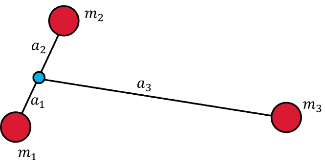
Figure 1: Orbital architecture of a planet on an S-Type orbit within a stellar binary, where the most massive component is $m_{1}$. The planetary and secondary star mass is represented by $m_{2}$ and $m_{3}$, respectively. The blue dot represents the center-of-mass for the inner pair, where planetary semimajor axis $a_{p}=a_{1}+a_{2}$ and the stellar semimajor axis $a_{\rm bin}=a_{3}$.

The three-body problem has no general solution (Poincaré, 1892), but we can make certain approximations due to the nature of our problem. The planetary mass is very small compared to either of the stellar masses so that we can apply a perturbation theory, which has been developed by Heppenheimer (1978), Marchal (1990), and Andrade-Ines and Eggl (2017) with varying complexity. Such analytical approaches are still useful despite the ubiquity of numerical simulations because they provide a more complete view and insights towards how the three-body system may change under slightly different initial conditions.

1 Secular evolution through a disturbing function

In the hierarchical case ($\alpha=(a_{p}/a_{\rm bin})\ll 1$), we can use the model by Heppenheimer (1978), which assumes there are no significant effects due to mean motion resonances. In this case the planet’s orbit will be altered by secular processes, which means that the eccentricity and/or orientation of the orbit can change, but not its semimajor axis (i.e., $\dot{a}_{p}\approx 0$). The secular interaction with the perturber $m_{3}$ is modeled through a Laplace-Lagrange disturbing function, which can be expanded in terms of the semimajor axis ratio $\alpha$ using Legendre polynomials $(P_{i})$, as $\alpha$ is a small parameter. In this model, we limit the expansion in Legendre polynomials to $P_{3}$ (i.e., quadrupole problem), which assumes that the planet’s eccentricity $e_{p}\ (=e_{2})$ is restricted to low values. Heppenheimer (1978) obtained the following secular disturbing function in orbital elements:

$$\mathcal{R}_{\rm Hep} =\frac{\mathcal{G}m_{3}}{\left(1-e_{\rm bin}^{2}\right)^{3/2}}\left(\frac{a_{p}}{a_{\rm bin}}\right)^{3}\left[\frac{1}{4}+\frac{3}{8}e_{p}^{2}-\frac{15}{16}\frac{a_{p}}{a_{\rm bin}}\frac{e_{p}e_{\rm bin}}{\left(1-e_{\rm bin}^{2}\right)}\cos(\Delta\varpi)\right],$$ (1)

where the subscript $p$ and ${\rm bin}$ refer to the planetary and binary orbital elements respectively. The relative longitude $\Delta\varpi\ (=\varpi_{p}-\varpi_{\rm bin})$ represents the relative orientation between the planetary and binary orbits within a reference plane. For simplicity, we assume that the stellar binary orbit is aligned along the $x$-axis so that $\varpi_{\rm bin}=0^{\circ}$.

In order to make the equations of motion linear and easier to solve, we introduce the planet’s eccentricity vector components as

$$\begin{aligned} k&=e_{p}\cos\Delta\varpi,\\ h&=e_{p}\sin\Delta\varpi,\end{aligned}$$ (2)

and using the planet’s mean motion $n_{p}=\sqrt{\mathcal{G}(m_{1}+m_{2})/a_{p}^{3}}$, and the semimajor axis ratio $\alpha=a_{p}/a_{\rm bin}$, we can rewrite Eq. 1 as

$$\mathcal{R}_{\rm Hep} =\frac{n_{p}^{2}a_{p}^{2}\alpha^{3}}{\left(1-e_{\rm bin}^{2}\right)^{3/2}}\left(\frac{m_{3}}{m_{1}+m_{2}}\right)\left[\frac{1}{4}+\frac{3}{8}\left(h^{2}+k^{2}\right)-\frac{15}{16}\frac{\alpha ke_{\rm bin}}{\left(1-e_{\rm bin}^{2}\right)}\right],$$ (3)

so that we can apply Hamilton’s equations:

$$\begin{aligned} \dot{k}&=-\frac{1}{n_{p}a_{p}^{2}}\frac{\partial R_{\rm Hep}}{\partial h},\\ \dot{h}&=\frac{1}{n_{p}a_{p}^{2}}\frac{\partial R_{\rm Hep}}{\partial k}.\end{aligned}$$ (4)

As a result, we find

$$\begin{aligned} \dot{k}&=-\frac{3}{4}\frac{n_{p}\alpha^{3}}{\left(1-e_{\rm bin}^{2}\right)^{3/2}}\left(\frac{m_{3}}{m_{1}+m_{2}}\right)h=-g_{H}h,\\ \dot{h}&=\frac{3}{4}\frac{n_{p}\alpha^{3}}{\left(1-e_{\rm bin}^{2}\right)^{3/2}}\left(\frac{m_{3}}{m_{1}+m_{2}}\right)\left[k-\frac{5}{4}\frac{\alpha e_{\rm bin}}{\left(1-e_{\rm bin}^{2}\right)}\right]=g_{H}\left[k-\epsilon_{H}\right],\end{aligned}$$ (5)

where $g_{H}$ represents a constant frequency and $\epsilon_{H}$ is an offset to the $k$ component of the eccentricity vector.

Using the method to solve coupled first-order equations produces

$$\begin{aligned} \ddot{h}+g_{H}^{2}h&=0,\\ \ddot{k}+g_{H}^{2}\left(k-\epsilon_{H}\right)&=0.\end{aligned}$$ (6)

Equation 6 has the form of a harmonic oscillator, which has the following analytical solutions:

$$\begin{aligned} k(t)&=e_{\rm free}\cos\left(g_{H}t+\phi\right)+\epsilon_{H},\\ h(t)&=e_{\rm free}\sin\left(g_{H}t+\phi\right),\end{aligned}$$ (7)

where $e_{\rm free}$ and $\phi$ is determined by the initial conditions $k(0)$ and $h(0)$. This method has introduced two additional parameters

$$\begin{aligned} g_{H}&=\frac{3}{4}\mu\alpha^{3}\frac{n_{p}}{\left(1-e_{\rm bin}^{2}\right)^{3/2}},\\ \epsilon_{H}&=\frac{5}{4}\alpha\frac{e_{\rm bin}}{\left(1-e_{\rm bin}^{2}\right)},\end{aligned}$$ (8)

where $\mu$ is the mass ratio $m_{3}/(m_{1}+m_{2})\approx m_{3}/m_{1}$, $g_{H}$ describes the precession frequency for a free eccentricity vector and $\epsilon_{H}$ is a stationary solution for the forced eccentricity vector induced from the stellar binary. These two vectors combine to give the planetary eccentricity vector (see Eq. 2), where $\Delta\varpi$ depends on time. The values of $e_{\rm free}$ and $\phi$ can be determined from the magnitude difference and orientation of the planetary eccentricity vector relative to the forced eccentricity vector. Mathematically, this is given by

$$\begin{aligned} e_{\rm free}&=\sqrt{\left[k(0)-\epsilon_{H}\right]^{2}+\left[h(0)\right]^{2}},\\ \tan\phi&=\frac{h(0)}{k(0)-\epsilon_{H}},\end{aligned}$$ (9)

where the arctan2 function should be used to find the value of $\phi$ in the proper quadrant.

Figure 2 illustrates the secular time evolution for three different initial planetary eccentricities $e_{po}$. Note that $\epsilon_{H}$ and $g_{H}$ do not depend on the initial planetary eccentricity where the differing amplitudes in each panel Fig. 2 depend on $e_{\rm free}$. Figs. 2a-2d show that one complete cycle completes in 36.5 yr, which corresponds to $2\pi/g_{H}$. The Heppenheimer model in the $(k,h)$ plane (Fig. 2e) shows the free eccentricity vector completing circular orbits with the end of the forced eccentricity vector as its origin. Note that the red circle $(e_{po}=0.03)$ has the smallest radius and the black circle has a larger radius.

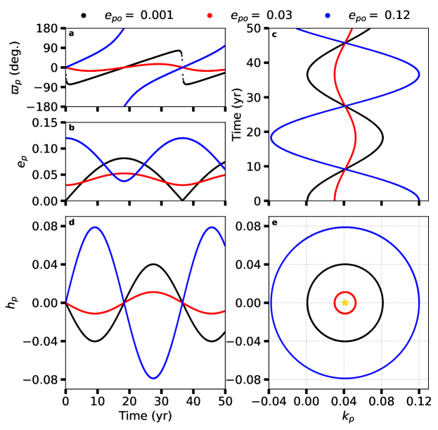
Figure 2: Secular time evolution for an S-Type planet using the Heppenheimer (1978) model, where $m_{1}=m_{3}=1\ M_{\odot}$, $\alpha=0.1$, $e_{\rm bin}=0.3$ for three different initial eccentricities $e_{po}$ initially aligned with the binary orbit $(\Delta\varpi=\varpi_{\rm bin}=0^{\circ})$. The gold star in panel e represents the forced eccentricity $\epsilon_{H}$, which does not depend on $e_{po}$. Figure adapted from (Andrade-Ines and Eggl, 2017).

The Heppenheimer model has limitations, where it fails once its main assumptions are broken (e.g., $e_{p}\gtrsim 0.1$ or $\alpha\gtrsim 0.2$). The Laplace-Lagrange formulation of the disturbing function is accurate to $\mathcal{O}(e_{2}^{2})$, where Marchal (1990) obtained a second-order solution in $\mu$ and $\alpha$ that is accurate to $\mathcal{O}(e_{2}^{3})$ with the appropriate corrections to $g_{H}$ and $\epsilon_{H}$ (see Georgakarakos, 2005; Andrade-Ines and Eggl, 2017). Although the disturbing function from Marchal’s model is move complicated, it can be simplified through the restricted problem $(m_{p}/m_{1}\rightarrow 0)$ and ignoring the terms of $\mathcal{O}(e_{p}^{3})$ to get

$$\mathcal{R}_{M}=n_{p}a_{p}^{2}g_{M}\left[\frac{1}{2}e_{p}^{2}-\epsilon_{M}e_{p}\cos\Delta\varpi\right],$$ (10)

where

$$g_{M} =g_{H}(1+\delta_{M}),$$ (11)

$$\epsilon_{M} =\epsilon_{H}(1+\delta_{M})^{-1},$$ (12)

$$\delta_{M} =\frac{25}{8}\frac{\mu\alpha^{3/2}}{\sqrt{1+\mu}}\frac{3+2e_{\rm bin}^{2}}{(1-e_{\rm bin}^{2})^{3/2}}.$$ (13)

Eventually, the Marchal approximation also breaks down, especially as $\alpha$ increases and other shorter period effects (e.g., mean motion resonances) are no longer negligible. An alternative approach is to introduce empirical corrections to $g_{H}$ and $\epsilon_{H}$ from a reference numerical solution and applying a fitting procedure in terms of $\alpha$, $\mu$, and $e_{\rm bin}$. Giuppone et al. (2011) demonstrated this method for the $\gamma$ Cephei system, where Andrade-Ines and Eggl (2017) generalized it to apply to eccentric binaries $(e_{\rm bin}\leq 0.6)$ and large mass ratios $(\mu\leq 10)$. The resulting approximation was limited to $N_{e}=15$ terms for the forced eccentricity correction and $N_{g}=18$ for the secular frequency. Each approximation can be represented as a finite sum by

$$\begin{aligned} \delta_{g}&=\sum_{i=1}^{N_{g}}A_{i}^{g}\alpha^{p_{i}^{g}}\mu^{q_{i}^{g}}e_{\rm bin}^{l_{i}^{g}},\\ \delta_{e}&=\sum_{i=1}^{N_{e}}A_{i}^{e}\alpha^{p_{i}^{e}}\mu^{q_{i}^{e}}e_{\rm bin}^{l_{i}^{e}},\end{aligned}$$ (14)

where

$$\begin{aligned} g_{AI}&=g_{H}(1+\delta_{g}),\\ \epsilon_{AI}&=\epsilon_{H}(1+\delta_{e}).\end{aligned}$$ (15)

The coefficients $A_{i}$ and corresponding exponents $(p_{i},\ q_{i},\ l_{i})$ are tabulated in Appendix A of Andrade-Ines and Eggl (2017). Note that when the mutual orbital inclination between the planet and the binary orbits is large $\gtrsim 40^{\circ}$, Von Zeipel-Lidov-Kozai oscillations can lead to large amplitude variations in planetary eccentricity and inclination (see discussions in section “stability in hierarchical systems” in chapter “Main-sequence systems: orbital stability around single star hosts”).

2 Applications of forced and free eccentricity

The forced and free eccentricity provide a good indicator for the stability of an exoplanet on an S-Type orbit. The forced eccentricity $\epsilon_{H}$ depends on the shape of the stellar binary’s orbit $(a_{\rm bin}$ and $e_{\rm bin})$ and the planetary semimajor axis $a_{p}$, since $\alpha=a_{p}/a_{\rm bin}$. This implies that the forced eccentricity sets a reference point for which the planetary eccentricity oscillates around (see Fig. 2). To ensure the stability of the exoplanet, its free eccentricity vector must be such that the eccentricity variation (i.e., amplitude relative to the forced eccentricity) is minimized.

The perturbation theory approach (in Sect. 1) to determine the forced eccentricity is an approximation, whereas we may need a more accurate estimate. In this case, we turn to numerical simulations that can efficiently forward-model a system given some initial parameters. Rebound has become a standard option due to its versatility and user-friendly interface that can be easily implemented on browser-based Jupyter notebooks.

Quarles et al. (2018a) applied a combination of numerical and secular methods for understanding planetary stability in the $\alpha$ Centauri system $(m_{A}=1.133\ M_{\oplus}$, $m_{B}=0.972\ M_{\oplus}$ and $e_{\rm bin}=0.524)$. Numerical n-body simulations provide a more complete solution, and in comparison to secular methods, we can see where the two begin to deviate. Suppose there is a exoplanet orbiting $\alpha$ Cen B with a semimajor axis $a_{p}=1.5$ au. The stability of the exoplanet depends on its initial eccentricity $e_{po}$ and relative orbital alignment $\Delta\varpi$ to the binary orbit that define its initial eccentricity vector. Quarles et al. (2018a) estimated, via n-body simulations, the forced eccentricity $e_{F}\approx 0.047$ using $\mu=1.165$, where the Marchal secular approximation produces $\epsilon_{M}=0.046$. These two methods match with an accuracy more than $99.5\%$, where the secular approximation is far less expensive computationally.

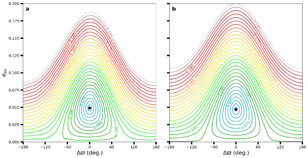
Figure 3: Maximum eccentricity (color-coded) for an S-Type exoplanet orbiting $\alpha$ Centauri B with a semimajor axis $a_{p}=1.5$ au with respect to the initial eccentricity $e_{po}$ and relative longitude $\Delta\varpi$ to the binary orbit. Panel (a) illustrates numerical results using Rebound, while panel (b) shows the results from perturbation theory using $\epsilon_{M}$ (Marchal, 1990) for the forced eccentricity. Figure adapted from (Quarles et al., 2018a).

However, the forced eccentricity is only one component, where we want to know the maximum eccentricity for which the planetary orbit can evolve. Equation 7 provides the components of the free eccentricity, where under secular evolution $e_{\rm max}=e_{\rm free}+e_{F}$ through vector addition. Figure 3 illustrates the differences between the two methods in the $(\Delta\varpi,e_{po})$ plane using the estimated maximum eccentricity (color-coded), where Fig. 3a is obtained through n-body simulation, and Fig. 3b is found using secular theory. Comparing Fig. 3a to Fig. 3b, we see a fixed point that represents the forced eccentricity at the expected location. The contours in Fig. 3a at high values of $e_{po}$ do not rise as high as those in Fig. 3b. This shows that secular approximation falls short in capturing the a complete picture for $e_{po}>0.1$ even with a more accurate estimate of the forced eccentricity.

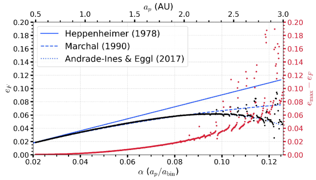
Figure 4: Forced eccentricity (black dots) for an S-Type exoplanet orbiting $\alpha$ Centauri B $(\mu=1.165)$ as a function of the initial semimajor ratio $\alpha$. The approximation from Heppenheimer (1978) overestimates $e_{F}$, where the approximation from Marchal (1990) fits well for $\alpha\lesssim 0.09$. The approximation from Andrade-Ines and Eggl (2017) captures the behavior for $\alpha>0.09$. Data taken from (Quarles et al., 2018a).

Using n-body simulations that minimize the eccentricity variation, we can estimate the forced eccentricity $e_{F}$ for a wide range in $\alpha$, where Quarles et al. (2018a) performed such simulations for a hypothetical planet in $\alpha$ Centauri AB. Figure 4 illustrates how the forced eccentricity determined by the n-body simulations (black dots) varies with $\alpha$, with an approximately quadratic growth. The goodness of the analytical approaches depends on how well the solid lines match the dots. From Eq. 7, we expect that the difference $e_{\rm max}-e_{F}$ is constant as both values would cancel each other to minimize the total eccentricity variation. However, Fig. 4 shows a growth in $e_{\rm max}-e_{F}$ (red dots), which demonstrates why the overall heights differed in Figure 3a and 3b. An additional ${\sim}0.0125$ in $e_{\rm max}$ is unaccounted for in the secular approximation.

This magnitude of $e_{\rm max}-e_{F}$ increases as $\alpha$ increases, but we can compare the approaches to estimate $e_{F}$ as that is independent of $e_{p}$ entirely. The blue curves in Fig. 4 show the predictions from each secular model, where all three converge as long as $\alpha\lesssim 0.035$. Unsurprisingly, the Heppenheimer model diverges first and overestimates $e_{F}$. The Marchal (1990) model is accurate up to $\alpha\sim 0.09$ (or $a_{p}\sim 2.125$, where the Andrade-Ines and Eggl (2017) model most accurately predicts the full range. Recall that the Andrade-Ines and Eggl (2017) model used a combination of numerical simulation and fitting techniques to determine its coefficients. Overall, this analysis shows that a planet bound to $\alpha$ Cen B could stably orbit as long as $\alpha\lesssim 0.105$ (or $a_{p}\lesssim 2.5$ au), although its orbit is likely eccentric $(e_{p}\sim 0.1)$ due to the stellar companion.

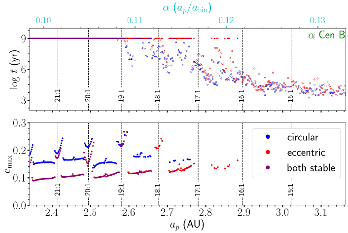
Figure 5: System lifetime $(\log\ t$; upper panel) and maximum eccentricity $(e_{\rm max}$; lower panel) for an S-Type exoplanet orbiting $\alpha$ Cen B as a function of the initial planetary semimajor axis $a_{p}$ through long-term (1 Gyr) n-body simulations. The exoplanet begins on either a circular orbit (blue dots) or at the forced eccentricity (red dots). Vertical lines denote the approximate locations for $N:1$ mean motion resonances. The top-axis provides a scale in terms of the semimajor axis ratio $\alpha$. Figure adapted from (Quarles et al., 2018a).

A stability transition region (sometimes referred to as grey) appears as the forcing from the stellar companion increases (i.e., large $\alpha$). Rabl and Dvorak (1988) introduced the boundaries of this grey region as the upper critical orbit (UCO) or lower critical orbit (LCO) using numerical simulations for only 300 orbits of the stellar binary. The transition from stable to unstable orbits is complicated by the choice for the initial planetary eccentricity, where either $e_{po}=0$ (circular) or $e_{po}=e_{F}$ (eccentric) appear as good choices. Figure 5 demonstrates the differences in the grey region’s extent through billion-year numerical simulations of a hypothetical exoplanet orbiting $\alpha$ Cen B. The maximum eccentricity for the planetary orbit is minimized for the initially eccentric (red dots) planetary orbits, while initially circular (blue dots) planetary orbits reach values about $50\%$ larger and even more for regions near $N:1$ mean motion resonances. Note that our earlier estimate (based on Fig. 4) for the beginning of the grey region (or stability transition boundary) was within ${\sim}5\%$ of the value obtained from 1 Gyr n-body simulations.

3 Stability through dynamical maps

Secular approximations for the stability of an exoplanet on a coplanar orbit around either component in a stellar binary has its limitations. Section 2 showed that the limitations become evident for large $(>0.1)$ values of $\alpha$, but approximations based on Eq. 8 can break down for circular binaries $(e_{\rm bin}=0)$. There are other tools from the circular restricted three-body problem (CRTBP) that help guide our inquiry into the planetary stability on S-Type orbits. The Jacobi constant (or the integral of relative energy) parametrizes the transition from stable to unstable orbits.

Eberle et al. (2008) developed a stability criterion in the CRTBP using the Jacobi constant $C_{J}$ and semimajor axis ratio $\alpha$. In the restricted problem, the planet does not affect the orbital evolution of the stellar binary ($m_{2}\rightarrow 0$), where it becomes more natural to redefine the binary mass ratio $\mu$ as

$$\mu^{\dagger} =\frac{m_{3}}{m_{1}+m_{3}}.$$ (16)

In barycentric coordinates, $\mu^{\dagger}$ represents the fractional part of the binary semimajor axis for which $m_{1}$ orbits the common center-of-mass $(a_{1}=\mu^{\dagger}a_{\rm bin})$. It also provides a more constrained definition for the mass ratio when the exoplanet orbits the other star $(0\leq\mu^{\dagger}\leq 1)$. When $\mu^{\dagger}<0.5$, the planet orbits $m_{1}$ and when $\mu^{\dagger}>0.5$, the masses $m_{1}$ and $m_{3}$ switch positions (assuming that $m_{1}>m_{3}$). The Jacobi constant (Eberle et al., 2008) is then computed as

$$C_{J}=\mu^{\dagger}+2\mu^{\dagger}\alpha+\frac{1-\mu^{\dagger}}{\alpha}+\frac{2\mu^{\dagger}}{1+\alpha}+2\sqrt{\alpha(1-\mu^{\dagger})},$$ (17)

which depends on $\mu^{\dagger}$ and the initial semimajor axis ratio $\alpha$, but not on any orbital parameter attained over the system’s evolution. The Jacobi constant $C_{J}$ also parametrizes the zero-velocity contour, which bounds the exoplanet trajectories absent any close approaches. Using the approximations for the collinear Lagrange equilibrium points, the Jacobi constant can be calculated for a particle at $L_{1}$, $L_{2}$, and $L_{3}$. Starting an exoplanet using $L_{1}$ correspondingly produces a $C_{1}$, which should limit the planetary stability because $L_{1}$ corresponds to a unstable point in the gravitational potential.

Numerical n-body simulations (Quarles et al., 2020) reveal that this is approximately true for inclined, prograde orbits. Jacobi constants at the other two collinear points $(L_{2}$ and $L_{3})$ provide more stringent limits in the $(\alpha,\mu^{\dagger})$ parameter space. Retrograde orbits $(i_{p}>90^{\circ})$ are not immune from this criterion, where $C_{3}$ bounds the stability the most. Figure 6 illustrates the stability of an exoplanet in the CRTBP for planetary inclinations of $0^{\circ}$, $30^{\circ}$, $45^{\circ}$, and $180^{\circ}$ relative to the binary orbital plane. The white regions are unstable, where the colored regions represent initial conditions that survive for at least $5\times 10^{5}$ yr.

Each panel is color-coded (on a logarithmic scale) with the maximum eccentricity attained over the full duration of system evolution. The orbits of low inclination planets (Figs. 6a and 6b) have maximum eccentricity $e_{\rm max}$ values that increase with $\alpha$, but are very much limited by the inner Lagrange point defined by the $C_{1}$ curve. Figure 6c displays a similar structure, but the orbits have a much larger maximum eccentricity (due to the octopole term in the Hamiltonian; von Zeipel (1910); Lidov (1962); Kozai (1962)) and is mostly independent of $\mu^{\dagger}$. Figure 6d shows that a retrograde orbiting exoplanet (i.e., orbiting opposite the direction of the stellar binary) can encompass much more of the $(\alpha,\mu^{\dagger})$ parameter space, but is still mostly bounded by the $C_{3}$ curve. The greater extent of stable retrograde orbits stems from a smaller average impulse imparted to the exoplanet on each passage of the stellar companion (e.g., Hamilton and Burns, 1991).

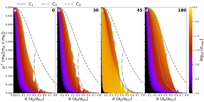
Figure 6: Stable configurations for an S-Type in the CRTBP (color-coded by $\log_{10}[e_{\rm max}$) with respect to the initial semimajor axis ratio $\alpha$ and mass ratio $\mu^{\dagger}$. Four different initial planetary inclinations $(i_{p}=0^{\circ},\ 30^{\circ},\ 45^{\circ},$ and $180^{\circ})$ are considered in panels a-d, where the unstable configurations are denoted by white cells. The gray contours correspond to the initial parameters that place the putative planet at one of the collinear Lagrange points $(L_{1},\ L_{2},\ L_{3})$. Figure adapted from (Quarles et al., 2020).

Using n-body simulations, Rabl and Dvorak (1988) identified stability regions considering exoplanets on S-Type orbits within eccentric binaries. Note that others (e.g., Chirikov, 1979) worked on quasi-analytic approaches to orbital stability based on Lyapunov characteristic numbers (Lyapunov, 1992) and chaos theory. The approach of Rabl and Dvorak developed a stability criterion for equal-mass binaries $(\mu^{\dagger}=0.5,$ also known as the Copenhagen problem) that depended on the semimajor axis $a_{p}$ of the putative exoplanet and the binary eccentricity $e_{\rm bin}$. They used relatively short (300 binary orbits) n-body simulations, but included eight equally spaced values in initial planetary longitude $\lambda_{p}$ and considered conditions where the binary began at its apastron or periastron position. From their results, Rabl and Dvorak performed a least-squares quadratic fit to obtain a critical semimajor axis ratio $\alpha_{c}\ (=a_{c}/a_{\rm bin})$,

$$\alpha_{c} =\begin{cases}(0.262\pm 0.006)-(0.254\pm 0.017)e_{\rm bin}-(0.060\pm 0.027)e_{\rm bin}^{2},&\text{(LCO)}\\ (0.336\pm 0.020)-(0.332\pm 0.051)e_{\rm bin}-(0.082\pm 0.082)e_{\rm bin}^{2},&\text{(UCO)}\end{cases}$$ (18)

for the lower critical orbit (LCO) and upper critical orbit (UCO), respectively. Note that the errors in the fitted coefficients can be very large, especially in the quadratic term $e_{\rm bin}^{2}$. Figure 7 illustrates the $(\alpha,e_{\rm bin})$ plane with the stability regions determined by Rabl and Dvorak (1988). The stable region represents initial conditions that are independent of the planet’s initial longitude $\lambda_{p}$ (i.e., all 8 trials survive the full simulation), where in the grey region some initial longitudes allow a planet to survive and other choices lead to escape. Figure 7 provides a reasonable estimate for the orbital stability, but it is limited to a single binary mass ratio and a modest range in binary eccentricity. These limitations reflect the computational capabilities of the time, where updates to the stability limit are possible proportionally to the advent of more efficient algorithms for orbital evolution and the greater availability of computing power.

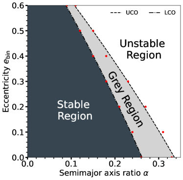
Figure 7: Stability regions for an S-Type exoplanet orbiting a single star in an equal-mass binary $(\mu^{\dagger}=0.5)$ with respect to the initial semimajor axis ratio $\alpha$ and binary eccentricity $e_{\rm bin}$. Red dots mark the critical semimajor axis ratio $\alpha_{c}$ using n-body simulations over 300 binary orbits and curves mark the least-squares fit (Eq. 18) determined by Rabl and Dvorak (1988). Figure adapted from (Rabl and Dvorak, 1988).

The stability criterion for exoplanets on S-Type orbits was revisited by Holman and Wiegert (1999), who expanded the approach to include a finer grid in trial values for the semimajor axis ratio $(0.02\leq\alpha\leq 0.50;$ with $\delta\alpha=0.01)$ and a range in the binary mass ratio $(0.1\leq\mu^{\dagger}\leq 0.9;$ with $\Delta\mu^{\dagger}=0.1)$. Additionally, the duration of a simulation by Holman and Wiegert was increased from 300 to $10^{4}$ binary orbits. This revision to the stability limit was possible due to the application of symplectic integration (Wisdom and Holman, 1992) to n-body simulations and a huge expansion of computing power in personal computers. Holman and Wiegert used eight equally-spaced values in the planetary longitude $\lambda_{p}$ following the procedure from Rabl and Dvorak (1988). Incorporating the additional parameter in the binary mass ratio, the revised formula for the stability limit became

$$\alpha_{c}= \ (0.464\pm 0.006)+(-0.380\pm 0.010)\mu^{\dagger}+(-0.631\pm 0.034)e_{\rm bin}+$$

$$\ (0.586\pm 0.061)\mu^{\dagger}e_{\rm bin}+(0.150\pm 0.041)e_{\rm bin}^{2}+(-0.198\pm 0.074)\mu^{\dagger}e_{\rm bin}^{2}.$$ (19)

Due to the relative simplicity of Eq. 3, it became widely used (for 20 years) as the standard for determining the orbital stability of exoplanets on S-Type orbits. Equation 3 is an empirical (not analytical) formula that is determined through many n-body simulations that make certain assumptions. Some of these assumptions are:

1. only three bodies exist in the system,

2. the simulation time $(10^{4}$ binary orbits) is sufficiently long,

3. the LCO boundary can be treated as the “stability limit”,

4. the mass $m_{2}$ can be treated as a test particle (i.e., $m_{2}\rightarrow 0)$,

5. all three bodies initially lie in the same plane (i.e., coplanar),

6. other effects on the planet’s motion (e.g., tides or general relativity) are negligible.

The known systems of binary stars with planets on S-Type orbits have not yet (largely) violated these assumptions, which has allowed the approach to remain in wide use.

Quarles et al. (2020) investigated how assumptions 2 and 5 affect the stability limit, as many of the confirmed planets on S-Type orbits do not lie in the stellar binary’s orbital plane. They also probe to finer ranges in $\mu^{\dagger}$, $e_{\rm bin}$, and $\alpha$, which allows for a revision to the formula for the stability limit through a similar least-squares procedure as Holman and Wiegert (1999) and Rabl and Dvorak (1988). For the coplanar case, the new stability formula is

$$\alpha_{c}= \ (0.501\pm 0.002)+(-0.435\pm 0.003)\mu^{\dagger}+(-0.668\pm 0.009)e_{\rm bin}+$$

$$\ (0.644\pm 0.015)\mu^{\dagger}e_{\rm bin}+(0.152\pm 0.011)e_{\rm bin}^{2}+(-0.196\pm 0.019)\mu^{\dagger}e_{\rm bin}^{2}$$ (20)

which largely revises the lower order terms in $\mu^{\dagger}$ and $e_{\rm bin}$ because Quarles et al. (2020) extended their range in mass ratio down to $\mu^{\dagger}=0.001$. Holman and Wiegert (1999) and Quarles et al. (2020) find similar values for the stability limit in $\alpha$ Centauri, which can be compared to more detailed studies of the system (e.g., Quarles and Lissauer, 2016). These previous investigations show that the stability limit is drastically different for highly inclined (relative to the binary orbital plane) planets.

Figure 8 illustrates how the critical semimajor axis $\alpha_{c}$ varies with the binary mass ratio $\mu^{\dagger}$ and eccentricity $e_{\rm bin}$. For coplanar orbits (Fig. 8a), the contours for the critical semimajor axis $\alpha_{c}$ do not appear to follow easily identifiable polynomials. Therefore, we may expect either empirical formula (Eq. 3 or 3) to fail near the edges of the map. Figure 8b is similar to Fig. 8a with slight distortions in the contours for a given $\alpha_{c}$. Figures 8c and 8d are even more distorted, where retrograde orbits (Fig. 8d) greatly enhance the extent of $\alpha_{c}$. In contrast, sufficiently inclined orbits in Fig. 8c show that the von Zeipel-Lidov-Kozai mechanism (von Zeipel, 1910; Lidov, 1962; Kozai, 1962)) is effective to excite the planetary orbit to very high values, which places an upper limit $\alpha{\sim}0.05$ in most cases.

Quarles and Lissauer (2018) investigated the stability of multiplanet systems, specifically in $\alpha$ Centauri, using a similar formalism for planet packing. Multiplanet systems need significantly more space between the planets due to the location of the single planet stability limit and the forced eccentricity from the stellar companion.

The process of optimizing a multivariate least-squares function tends to settle on coefficients that represent the median case (i.e., $\mu^{\dagger}{\sim}0.5$ and $e_{\rm bin}{\sim}0.5$). Applications of the above empirical formulas towards high $(\mu^{\dagger}>0.9$) or low $(\mu^{\dagger}<0.1)$ mass ratio give less accurate results when compared with n-body simulations specific to those ranges. To avoid these issues, Quarles et al. (2020) provided a publicly available lookup table, where interpolation routines from scipy.interpolate can be implemented to provide accurate results and potentially go beyond the given grid resolution. An example is shown as:

[chap1:box1]Example 2D interpolation code in python

⬇

from scipy.interpolate import CloughTocher2DInterpolator

import numpy as np

mu = 0.05

e_bin = 0.5

Quarles_repo = ”https://raw.githubusercontent.com/saturnaxis/ThreeBody_Stability/master/”

fn = ”a_crit_Incl[0].txt”

X, Y, Z = np.genfromtxt(Quarles_repo + fn,delimiter=’,’,comments=’#’,unpack=True)

interp = CloughTocher2DInterpolator(np.array([X,Y]).T, Z)

print(”a_c␣=␣”,interp(mu,e_bin))

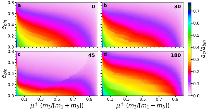
Figure 8: Critical semimajor axis $\alpha_{c}$ (color-coded) as a function of the binary eccentricity $e_{bin}$ and the mass ratio $\mu^{\dagger}$. The initial planetary inclination $i_{p}$ (in degrees) of the S-Type planet is denoted in each panel in the upper right. Figure adapted from (Quarles et al., 2020).

3 P-type stability

Planets on P-Type orbits may appear more familiar because such planets orbit both stars completely (see Fig. 9). This orbital architecture is actually similar to the S-Type orbits describe in Section 2. Let us consider Figure 1, but define $m_{2}=m_{B}$ (the stellar companion’s mass) and $m_{3}=m_{p}$ (the planetary mass). Consequently, the semimajor axes are also redefined with $a_{\rm bin}=a_{1}+a_{2}$ and $a_{3}=a_{p}$. By doing so, we have effectively switched indices in the hierarchy and are able to re-use many of the same theoretical concepts and techniques.

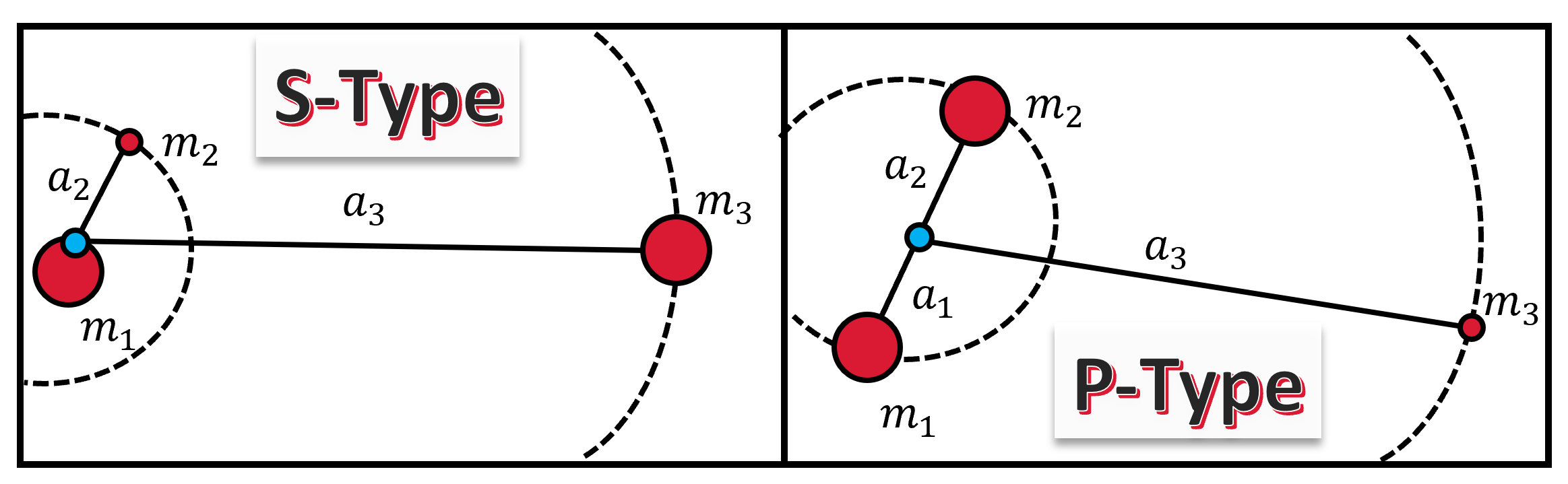
Figure 9: Schematic illustrating the difference between planets in either S-Type (left) or P-Type (right) orbits. The stellar masses are represented as the larger dots, where the planet is the smaller dot in each panel.

1 Secular evolution through a disturbing function

A planet’s orbit can change secularly, assuming that the planet begins far from the inner region that is dominated by the N:1 mean motion resonances with the binary (i.e., $a_{p}\gg a_{\rm bin}$. In this formulation, we also make the same assumptions that the planetary eccentricity and/or orientation evolve while variations in the semimajor axis are negligible (i.e., $\dot{a}_{p}\approx 0)$. The secular interaction with the inner binary is modeled using a Laplace-Lagrange disturbing function, which can be expanded in terms of the semimajor axis ratio $(a_{p}/a_{\rm bin})$ using Legendre polynomials $(P_{i})$. In the quadrupole limit, Moriwaki and Nakagawa (2004) obtained the following secular disturbing function in orbital elements:

$$\mathcal{R}_{\rm MN}=\mu^{\dagger}(1-\mu^{\dagger})n_{\rm bin}^{2}a_{\rm bin}^{2}\left(\frac{a_{p}}{a_{\rm bin}}\right)^{-3}\left[\frac{1}{4}\left(1+\frac{3}{2}e_{p}^{2}\right)\left(1+\frac{3}{2}e_{\rm bin}^{2}\right)-\frac{15}{16}\left(1-2\mu^{\dagger}\right)\left(\frac{a_{p}}{a_{\rm bin}}\right)^{-1}e_{p}\left(e_{\rm bin}+\frac{3}{4}e_{\rm bin}^{3}\right)\cos\Delta\varpi\right],$$ (21)

where the subscript $p$ and $\rm bin$ refer to the planetary and binary orbital elements, respectively. Note that Eq. 21 is truncated in a similar manner as Eq. 10 in the S-Type case. The relative longitude $\Delta\varpi\ (=\varpi_{p}-\varpi_{\rm bin})$ represents the relative orientation between the planetary and binary orbits within a reference plane. The binary mass ratio $\mu^{\dagger}\ \left[=m_{B}/(m_{A}+m_{B})\right]$ and mean motion $n_{\rm bin}\ \left(=\sqrt{G(m_{A}+m_{B})/a_{\rm bin}^{2}}\right)$ are used as prefactors due to our switching of indices in the setup of the orbital architecture. Note that this disturbing function has a similar structure as Eq. 1, where the higher order terms in $e_{p}$ and $e_{\rm bin}$ are ignored.

Using the eccentricity vector components in Eq. 2, the $\cos(a-b)$ trigonometric identity, and the semimajor axis ratio $\alpha\ (=a_{p}/a_{\rm bin})$, the disturbing function (Eq. 21) is rewritten as

$$\begin{aligned} \mathcal{R}_{\rm MN}=\mu^{\dagger}(1-\mu^{\dagger})n_{\rm bin}^{2}a_{\rm bin}^{2}\alpha^{-3}\left[\frac{1}{4}\left(1+\frac{3}{2}h^{2}+\frac{3}{2}k^{2}\right)\left(1+\frac{3}{2}e_{\rm bin}^{2}\right)-\frac{15}{16}\left(1-2\mu^{\dagger}\right)\alpha^{-1}e_{p}\left(e_{\rm bin}+\frac{3}{4}e_{\rm bin}^{3}\right)\left(k\cos\varpi_{\rm bin}-h\sin\varpi_{\rm bin}\right)\right],\end{aligned}$$ (22)

so that we can apply Hamilton’s equations (Eq. 4) to get

$$\begin{aligned} \dot{k}&=-g_{MN}h-B\sin\varpi_{\rm bin},\\ \dot{h}&=g_{MN}k-B\cos\varpi_{\rm bin},\end{aligned}$$ (23)

where

$$g_{MN} =\frac{3}{4}\mu^{\dagger}\left(1-\mu^{\dagger}\right)\alpha^{-5}\frac{n_{\rm bin}^{2}}{n_{p}}\left(1+\frac{3}{2}e_{\rm bin}^{2}\right),$$ (24)

$$B =\frac{5}{4}\left(1-2\mu^{\dagger}\right)g_{MN}\alpha^{-1}e_{\rm bin}\left[\frac{1+(3/4)e_{\rm bin}^{2}}{1+(3/2)e_{\rm bin}^{2}}\right].$$ (25)

Using the method to solve coupled first-order equations, we find equations that resemble a forced harmonic oscillator as:

$$\begin{aligned} \ddot{h}+g_{MN}^{2}h&=-g_{MN}B\sin\varpi_{\rm bin},\\ \ddot{k}+g_{MN}^{2}k&=-g_{MN}B\cos\varpi_{\rm bin},\end{aligned}$$ (26)

which has the analytical solutions:

$$\begin{aligned} k(t)&=e_{\rm free}\cos(g_{MN}t+\varphi)+\epsilon_{MN}\cos\varpi_{\rm bin},\\ h(t)&=e_{\rm free}\sin(g_{MN}t+\varphi)+\epsilon_{MN}\sin\varpi_{\rm bin}\end{aligned}$$ (27)

, where $e_{\rm free}$ and $\varphi$ are determined by the initial conditions $k(0)$ and $h(0)$. The forced eccentricity $\epsilon_{MN}$ is given by

$$\epsilon_{MN} =\frac{B}{g_{MN}}=\frac{5}{4}\left(1-2\mu^{\dagger}\right)\alpha^{-1}e_{\rm bin}\left[\frac{1+(3/4)e_{\rm bin}^{2}}{1+(3/2)e_{\rm bin}^{2}}\right].$$ (28)

This secular approximation is applicable to a broad range of cases, but it clearly has limits. For example, the symmetric cases $e_{\rm bin}$ (circular binary) or $\mu^{\dagger}=0.5$ (equal mass binary) result in $\epsilon_{MN}=0$. N-body simulations of disks (using test particles) show that a forced eccentricity exists that pumps the eccentricity of disk particles (Moriwaki and Nakagawa, 2004).

Figure 10 illustrates the secular evolution (assuming three initial eccentricities) of a hypothetical planet in a P-Type orbit, where $m_{1}=1\ M_{\odot}$, $m_{2}=0.3\ M_{\odot}$, $\alpha=5$, and $e_{\rm bin}=0.3$. The evolution using the Moriwaki and Nakagawa model appears similar to Fig. 2, however the planet is initially misaligned with the binary orbit $(\Delta\varpi=45^{\circ})$. This offsets the evolution of the planetary longitude of pericenter $\varpi_{p}$ (Fig. 10a), and the eccentricity vectors $k_{p}$ (Fig. 10c) and $h_{p}$ (Fig. 10d). As a result, the center point (gold star in Fig. 10e) is rotated (counter-clockwise) by $\varpi_{\rm bin}$.

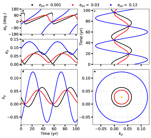
Figure 10: Secular time evolution for an P-Type planet using the Moriwaki and Nakagawa (2004) model, where $m_{1}=1\ M_{\odot}$, $m_{2}=0.3\ M_{\odot}$, $\alpha=5$, $e_{\rm bin}=0.3$ for three different initial eccentricities $e_{po}$ initially misaligned with the binary orbit $(\Delta\varpi=\varpi_{\rm bin}=45^{\circ})$. The gold star in panel e represents the forced eccentricity $\epsilon_{MN}$, which does not depend on $e_{po}$.

2 Applications of forced and free eccentricity

Similar to Sec. 2, the forced and free eccentricity can provide a good indicator for the stability of an exoplanet on a P-Type orbit. The forced eccentricity $\epsilon_{MN}$ depends on the shape of the stellar binary’s orbit $(a_{\rm bin}$ and $e_{\rm bin})$ and the planetary semimajor axis $a_{p}$, since $\alpha=a_{p}/a_{\rm bin}$. However, the forced eccentricity is expanded in inverse powers using the ratio $\alpha$ since $a_{p}\gg a_{\rm bin}$. The forced eccentricity sets a reference point for which the planetary eccentricity oscillates around (see Fig. 10).

Moriwaki and Nakagawa (2004), Paardekooper et al. (2012), and Demidova and Shevchenko (2015) used calculations of the forced eccentricity to better understand structures within circumbinary protoplanetary disks. Paardekooper et al. (2012) investigated planet formation of the newly discovered “Tatooine” exoplanets from the Kepler Space telescope, in which they derive a fast component to describe a growing planet’s eccentricity evolution by averaging over the mean longitude of the inner binary only (instead of averaging over both) in the disturbing function. As a result, they obtained a fast version of the forced eccentricity $\epsilon_{ff}$, where

$$\epsilon_{ff} =\frac{3}{4}\mu^{\dagger}\left(1-\mu^{\dagger}\right)\alpha^{-2}\sqrt{1+\frac{34}{3}e_{\rm bin}^{2}}.$$ (29)

Note that $\epsilon_{ff}$ falls off faster than $e_{MN}$ (Eq. 28) as $\alpha$ increases. Demidova and Shevchenko (2015) used the forced eccentricity $\epsilon_{MN}$ to model eccentricity variations and spiral patterns of particles within the circumbinary protoplanetary disk, where $e_{p}=2\epsilon_{MN}|\sin(g_{MN}t)|$. Through this model, one can approximate the time-averaged eccentricity as a combination of the fast $\epsilon_{ff}$ and slow $\epsilon_{MN}$ components (Shevchenko, 2018), or

$$\langle e_{p}\rangle=\frac{4}{\pi}\left(\epsilon_{MN}+\epsilon_{ff}\right).$$ (30)

Using n-body simulations that minimize the eccentricity variation, we can estimate the forced eccentricity $e_{F}$ for a wide range in $\alpha$, where Quarles et al. (2018a) performed such simulations for a hypothetical circumbinary planet in $\alpha$ Centauri AB $(\mu^{\dagger}=0.461$, $e_{\rm bin}=0.524$, and $a_{\rm bin}=23.78\ {\rm au})$. Figure 11 illustrates how the forced eccentricity (black dots) and maximum eccentricity (red dots) determined by n-body simulations varies with $\alpha$, where the magnitude of each decays with increasing $\alpha$. The secular approximation from Moriwaki and Nakagawa (2004) (solid blue line) is accurate for $\alpha\gtrsim 4$, but underestimates forced eccentricity $e_{F}$ for planets closer to the inner binary due to additional effects (e.g., $N$:1 mean motion resonances). The dashed blue line shows the approximation $\langle e_{p}\rangle$ using both approximations for the forced eccentricity, which closely approximates $e_{\rm max}$ for $\alpha\gtrsim 4$. However, the ratio $e_{\rm max}/e_{F}$ converges to 5 rather than 2, as we would expect from the addition of the free and forced eccentricity vectors.

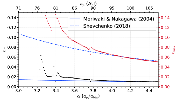
Figure 11: Forced eccentricity (black dots) for a P-Type exoplanet orbiting $\alpha$ Centauri AB $(\mu^{\dagger}=0.461)$ as a function of the initial semimajor ratio $\alpha$. The approximation (Eq. 28) from Moriwaki and Nakagawa (2004) underestimates $e_{F}$ when $\alpha\lesssim 4$. The approximation from Shevchenko (2018) captures the behavior of $e_{\rm max}$ for $\alpha\gtrsim 4$. Data taken from (Quarles et al., 2018a).

3 Stability through dynamical maps

Similar to S-Type systems, exoplanets on P-Type orbits also suffer limitations when using the secular approximation. In particular, Eq. 28 goes to zero when the binary orbit is circular or for equal-mass binaries (i.e., $\mu^{\dagger}=0.5)$. Other works have provided a more detailed expansion in which other forcing terms are included. These expansions have informed the studies of circumbinary planets (Li et al., 2014) and the evolution of Pluto’s smaller moons (Bromley and Kenyon, 2015). However, these other terms in the expansion depend on factors of

$$\frac{m_{1}-m_{2}}{m_{1}+m_{2}} =1-2\mu^{\dagger},$$

which goes to zero, when $\mu^{\dagger}=0.5$. Equal-mass binaries appear symmetric in the secular potential, where $e_{F}\approx 0$ makes sense. But, other (non-secular) factors persist to perturb a circumbinary planet so that its orbit is highly eccentric (see Fig. 11 at $\alpha=3.2-3.4$).

To explore all possible cases, we again turn to n-body simulations and how those numerical solutions have helped to provided a more general criterion for orbital stability. Dvorak (1986) developed a stability criterion that for equal-mass binaries $(\mu^{\dagger}=0.5)$ that depended only on the binary eccentricity $e_{\rm bin}$ and planetary semimajor axis $a_{p}$ to produce the critical semimajor axis ratio $\alpha\ (=a_{p}/a_{\rm bin})$. At the time and sometimes even now, an exact definition of orbital stability is not always given. It is important to note that Dvorak contended with two definitions:

1. ”A stable orbit is defined as an orbit having elliptic orbital elements with an eccentricity smaller than 0.3 throughout the whole integration time of 500 periods of the primary bodies.”

2. ”All solutions stay in bounded regions of the phase space and no collisions and no escapes of the bodies occur.”

The first definition is more precise, but the conditions given (e.g., $\text{max}\ e_{p}<0.3$) were defined relative to numerical experience. But, the perturbations act in a similar way on the orbital elements of stable and unstable trajectories alike for the ”escape” orbits within the phase space so that the second definition is also found wanting. We include this dilemma to show the importance of including your assumptions and that trade-offs are often necessary with limited resources.

Dvorak used short (400 binary orbits) n-body simulations, but included ten equally-spaced values in the initial planetary longitude $\lambda_{p}$ and considered conditions where the binary began at its apastron or periastron position; the approach in Rabl and Dvorak (1988) was based on this technique. From his results, Dvorak used a least-squares quadratic fit to obtain two relations for the critical semimajor axis,

$$\alpha_{c} =\begin{cases}(2.09\pm 0.30)+(2.79\pm 0.53)e_{\rm bin}-(2.08\pm 0.56)e_{\rm bin}^{2},&\text{(LCO)}\\ (2.37\pm 0.23)+(2.76\pm 0.40)e_{\rm bin}-(1.04\pm 0.43)e_{\rm bin}^{2},&\text{(UCO)}\end{cases}$$ (31)

for the lower critical orbit (LCO) and upper critical orbit (UCO), respectively. Figure 12 shows the $(\alpha,\ e_{\rm bin})$ plane with the stability regions determined by Dvorak (1986). The stable region represents where initial conditions are independent of the planet’s initial longitude $\lambda_{p}$ (i.e., all 10 trials survive the full simulation), where in the grey region some initial longitudes allow a planet to survive while others initial values lead to escape.

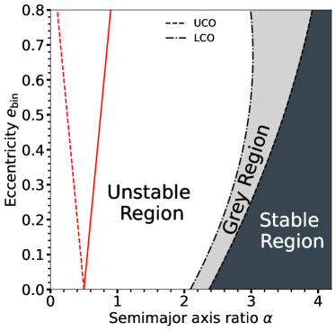
Figure 12: Stability regions for equal-mass binary $(\mu^{\dagger}=0.5)$ with respect to the initial semimajor axis ratio $\alpha$ and binary eccentricity $e_{\rm bin}$. The dashed and dash-dot curves mark the least-squares fit (Eq. 31) determined by Dvorak (1986). The red curves illustrate the relative proximity (relative to the binary semimajor axis) of the secondary star at apastron (solid) or periastron (dashed). Figure adapted from Dvorak (1986).

Similar to S-Type orbits, the stability criterion for exoplanets on P-Type orbits was revisited by Holman and Wiegert (1999), who expanded the approach to include a finer grid in trial values for the semimajor axis ratio $(1\leq\alpha\leq 5;$ with $\delta\alpha=0.1)$ and a range in the binary mass ratio $(0.1\leq\mu^{\dagger}\leq 0.5;$ with $\Delta\mu^{\dagger}=0.1)$. Additionally, the duration of a simulation by Holman and Wiegert was increased from 400 to $10^{4}$ binary orbits due to the application of symplectic integration (Wisdom and Holman, 1992) to n-body simulations and a huge expansion of computing power in personal computers. Holman and Wiegert used eight equally-spaced values in the planetary longitude $\lambda_{p}$ following the procedure from Dvorak (1986). Incorporating the additional parameter in the binary mass ratio, the revised formula for the stability limit became

$$\alpha_{c}= \ (1.60\pm 0.04)+(4.12\pm 0.09)\mu^{\dagger}+(5.10\pm 0.05)e_{\rm bin}+(-4.27\pm 0.17)\mu^{\dagger}e_{\rm bin}+$$

$$\ (-2.22\pm 0.11)e_{\rm bin}^{2}+(-5.09\pm 0.11)\left(\mu^{\dagger}\right)^{2}+(4.61\pm 0.36)\left(\mu^{\dagger}e_{\rm bin}\right)^{2}.$$ (32)

Due to the relative simplicity of Eq. 3, it became widely used (for 20 years) as the standard for determining the orbital stability of exoplanets on P-Type orbits. Equation 3 is an empirical (not analytical) formula that is determined through many n-body simulations that make certain assumptions. Most of the same assumptions outlined in Sec. 3 apply, except assumption #3 uses the UCO boundary instead.

Quarles et al. (2018b) investigated how assumptions $1-4$ affect our estimate of the stability limit and how the newly discovered circumbinary planets span the $(\mu^{\dagger},\ e_{\rm bin})$ plane for orbital stability. Note that Kepler-47 is a 3 planet circumbinary system (Orosz et al., 2019), where only 2 planets were known at the time of initial discovery (Orosz et al., 2012). The 2 planet solution to Kepler-47 motivated Quarles et al. (2018b) to use methods developed in the chapter for compact systems orbiting single stars to account for the outer planet’s influence on the orbital stability of the inner planet.

For the stability limit in single planet systems, Quarles et al. (2018b) probed to finer ranges in $\mu^{\dagger}$, $e_{\rm bin}$, and $\alpha$ compared to Holman and Wiegert (1999). This allowed for a revision to the empirical formula for the stability limit through a similar least-squares procedure as Holman and Wiegert (1999). The new stability formula is

$$\alpha_{c}= \ (1.48\pm 0.01)+(5.14\pm 0.10)\mu^{\dagger}+(3.92\pm 0.06)e_{\rm bin}+(0.33\pm 0.19)\mu^{\dagger}e_{\rm bin}+$$

$$\ (-1.41\pm 0.06)e_{\rm bin}^{2}+(-7.95\pm 0.15)\left(\mu^{\dagger}\right)^{2}+(-4.89\pm 0.44)\left(\mu^{\dagger}e_{\rm bin}\right)^{2},$$ (33)

which substantially differs from the coefficients determined by Holman and Wiegert. This difference occurs because Quarles et al. (2018b) extended their range in mass ratio down to $\mu^{\dagger}=0.001$. Figure 13 illustrates how the critical semimajor axis $\alpha_{c}$ varies with the binary mass ratio $\mu^{\dagger}$ and eccentricity $e_{\rm bin}$. The contours in this map are mostly flat with the binary eccentricity in the middle $(\mu^{\dagger}=0.1-0.4)$, where larger deviations occur at the extremes in mass ratio. This demonstrates that empirical formulas (Eq. 3 or 3) will likely be insufficient in the regimes where $\mu^{\dagger}<0.1$ or $\mu^{\dagger}>0.4$. Figure 13 shows that about half of the known circumbinary planets discovered using either the Kepler Space telescope or the Transiting Exoplanet Survey Satellite (TESS; Ricker et al. (2015)) lie within the high mass ratio regime. To avoid this complication, Quarles et al. (2018b) provided a publicly available lookup table, where interpolation routines from scipy.interpolate can be implemented to provide accurate results and potentially go beyond the given grid resolution. An example is as:

[chap1:box2]Example 2D interpolation code in python

⬇

from scipy.interpolate import CloughTocher2DInterpolator

import numpy as np

mu = 0.05

e_bin = 0.5

Quarles_repo = ”https://raw.githubusercontent.com/saturnaxis/CBP_stability/master/”

fn = ”a_crit.txt”

X, Y, Z = np.genfromtxt(Quarles_repo + fn,delimiter=’,’,comments=’#’,unpack=True)

interp = CloughTocher2DInterpolator(np.array([X,Y]).T, Z)

print(”a_c␣=␣”,interp(mu,e_bin))

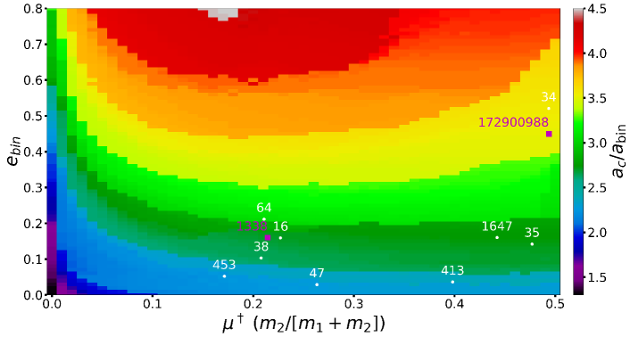
Figure 13: Critical semimajor axis $\alpha_{c}$ (color-coded) of a P-Type exoplanet as a function of the binary eccentricity $e_{bin}$ and the mass ratio $\mu^{\dagger}$ ($m_{1}$ and $m_{2}$ are the stellar masses). The white dots (and numbers) mark the system parameters for the circumbinary planets discovered using the Kepler Space telescope. The magenta squares mark the confirmed system (TOI-1338; Kostov et al. (2020)) and planet candidate (TIC 172900988; Kostov et al. (2021)) discovered using TESS (Ricker et al., 2015). Figure adapted from (Quarles et al., 2018b).

Lam and Kipping (2018) used a deep neural network (DNN) trained on a million n-body simulations to characterize the stability limit. The DNN technique provided a machine-learning approach that contrasts to the ${\sim}10^{8}$ simulations required to produce a general map like Fig. 13. There are limitations to the DNN approach, where it had a recall accuracy of ${\sim}90\%$ that is likely a trade-off from having a smaller training set. Using either a lookup table or a DNN is a good first step to estimating the stability limit, where the details (e.g., number of planets, inclined planets, mean motion resonances) are likely to be system specific. More recently, Georgakarakos et al. (2024) revisited the problem of the dynamical stability of hierarchical triple systems with applications to circumbinary planetary orbits. They provided empirical expressions in the form of multidimensional, parameterized fits for the two borders that separate the three dynamical domains, and trained a machine learning model on the data set in order to have an alternative tool of predicting the stability of circumbinary planets.

4 Conclusion

This chapter has reviewed the intricate dynamics and stability of planetary systems within binary star environments, an area of study that holds important implications for our understanding of exoplanetary systems. Through a combination of secular methods, N-body simulations, and the application of machine learning techniques, one can analyze the stability of S-type (planets orbiting one star) and P-type (planets orbiting both stars) configurations in binary systems.

Our chapter highlights the critical role of gravitational interactions between stellar components and their orbiting planets, which dictate the long-term stability of these systems. The Laplace-Lagrange framework and disturbing functions have been instrumental in deriving key insights into the secular evolution of planetary orbits (e.g., Heppenheimer, 1978; Marchal, 1990; Moriwaki and Nakagawa, 2004; Andrade-Ines and Eggl, 2017). By defining critical orbits and stability boundaries, one can identify regions where planets can maintain stable trajectories over extended periods.

The necessity of numerical simulations is underscored by their ability to capture the full complexity of planetary dynamics in binary systems (Rabl and Dvorak, 1988; Quarles et al., 2018a, 2020). These simulations, augmented by machine learning models, have significantly enhanced our predictive capabilities, allowing for high-accuracy stability assessments (Lam and Kipping, 2018) The integration of these advanced methodologies has provided a more comprehensive understanding of the dynamic interactions at play.

As the discovery of exoplanets within binary star systems continues, the frameworks and methods discussed in this chapter will be essential for future research. Understanding the balance of forces that govern planetary stability in these complex environments not only advances our knowledge of celestial mechanics but also informs the characterization of exoplanetary systems.

45

Andrade-Ines E and Eggl S (2017), Apr. Secular Orbit Evolution in Systems with a Strong External Perturber - A Simple and Accurate Model. AJ 153 (4), 148. 10.3847/1538-3881/153/4/148. 1701.03425.

Bromley BC and Kenyon SJ (2015), Aug. Evolution of a Ring around the Pluto-Charon Binary. ApJ 809 (1), 88. 10.1088/0004-637X/809/1/88. 1503.06805.

Campbell B, Walker GAH and Yang S (1988), Aug. A Search for Substellar Companions to Solar-type Stars. ApJ 331: 902. 10.1086/166608.

Chambers JE, Quintana EV, Duncan MJ and Lissauer JJ (2002), May. Symplectic Integrator Algorithms for Modeling Planetary Accretion in Binary Star Systems. AJ 123 (5): 2884–2894. 10.1086/340074.

Chirikov BV (1979), May. A universal instability of many-dimensional oscillator systems. Phys. Rep. 52 (5): 263–379. 10.1016/0370-1573(79)90023-1.

Cincotta P and Simó C (1999), Jan. Conditional Entropy. Celestial Mechanics and Dynamical Astronomy 73: 195–209. 10.1023/A:1008355215603.

Demidova TV and Shevchenko II (2015), May. Spiral Patterns in Planetesimal Circumbinary Disks. ApJ 805 (1), 38. 10.1088/0004-637X/805/1/38. 1407.5493.

Doyle LR, Carter JA, Fabrycky DC, Slawson RW, Howell SB, Winn JN, Orosz JA, Přsa A, Welsh WF, Quinn SN, Latham D, Torres G, Buchhave LA, Marcy GW, Fortney JJ, Shporer A, Ford EB, Lissauer JJ, Ragozzine D, Rucker M, Batalha N, Jenkins JM, Borucki WJ, Koch D, Middour CK, Hall JR, McCauliff S, Fanelli MN, Quintana EV, Holman MJ, Caldwell DA, Still M, Stefanik RP, Brown WR, Esquerdo GA, Tang S, Furesz G, Geary JC, Berlind P, Calkins ML, Short DR, Steffen JH, Sasselov D, Dunham EW, Cochran WD, Boss A, Haas MR, Buzasi D and Fischer D (2011), Sep. Kepler-16: A Transiting Circumbinary Planet. Science 333 (6049): 1602. 10.1126/science.1210923. 1109.3432.

Dvorak R (1982), Jan. Planetenbahnen in Doppelsternsystemen. Oesterreichische Akademie Wissenschaften Mathematisch naturwissenschaftliche Klasse Sitzungsberichte Abteilung 191 (10): 423–437.

Dvorak R (1986), Oct. Critical orbits in the elliptic restricted three-body problem. A&A 167: 379–386.

Eberle J, Cuntz M and Musielak ZE (2008), Oct. The instability transition for the restricted 3-body problem. I. Theoretical approach. A&A 489 (3): 1329–1335. 10.1051/0004-6361:200809758.

Georgakarakos N (2005), Sep. Erratum: Eccentricity evolution in hierarchical triple systems with eccentric outer binaries. MNRAS 362 (2): 748–748. 10.1111/j.1365-2966.2005.09441.x.

Georgakarakos N, Eggl S, Ali-Dib M and Dobbs-Dixon I (2024), Apr. Empirical stability criteria for 3D hierarchical triple systems I: Circumbinary planets. arXiv e-prints , arXiv:2404.1374610.48550/arXiv.2404.13746. 2404.13746.

Giuppone CA, Leiva AM, Correa-Otto J and Beaugé C (2011), Jun. Secular dynamics of planetesimals in tight binary systems: application to $\gamma$-Cephei. A&A 530, A103. 10.1051/0004-6361/201016375. 1105.0243.

Hamilton DP and Burns JA (1991), Jul. Orbital stability zones about asteroids. Icarus 92 (1): 118–131. 10.1016/0019-1035(91)90039-V.

Heppenheimer TA (1978), May. On the formation of planets in binary star systems. A&A 65 (3): 421–426.

Holman MJ and Wiegert PA (1999), Jan. Long-Term Stability of Planets in Binary Systems. AJ 117 (1): 621–628. 10.1086/300695. astro-ph/9809315.

Kostov VB, Orosz JA, Feinstein AD, Welsh WF, Cukier W, Haghighipour N, Quarles B, Martin DV, Montet BT, Torres G, Triaud AHMJ, Barclay T, Boyd P, Briceno C, Cameron AC, Correia ACM, Gilbert EA, Gill S, Gillon M, Haqq-Misra J, Hellier C, Dressing C, Fabrycky DC, Furesz G, Jenkins JM, Kane SR, Kopparapu R, Hodžić VK, Latham DW, Law N, Levine AM, Li G, Lintott C, Lissauer JJ, Mann AW, Mazeh T, Mardling R, Maxted PFL, Eisner N, Pepe F, Pepper J, Pollacco D, Quinn SN, Quintana EV, Rowe JF, Ricker G, Rose ME, Seager S, Santerne A, Ségransan D, Short DR, Smith JC, Standing MR, Tokovinin A, Trifonov T, Turner O, Twicken JD, Udry S, Vanderspek R, Winn JN, Wolf ET, Ziegler C, Ansorge P, Barnet F, Bergeron J, Huten M, Pappa G and van der Straeten T (2020), Jun. TOI-1338: TESS’ First Transiting Circumbinary Planet. AJ 159 (6), 253. 10.3847/1538-3881/ab8a48. 2004.07783.

Kostov VB, Powell BP, Orosz JA, Welsh WF, Cochran W, Collins KA, Endl M, Hellier C, Latham DW, MacQueen P, Pepper J, Quarles B, Sairam L, Torres G, Wilson RF, Bergeron S, Boyce P, Bieryla A, Buchheim R, Ben Christiansen C, Ciardi DR, Collins KI, Conti DM, Dixon S, Guerra P, Haghighipour N, Herman J, Hintz EG, Howard WS, Jensen ELN, Kielkopf JF, Kruse E, Law NM, Martin D, Maxted PFL, Montet BT, Murgas F, Nelson M, Olmschenk G, Otero S, Quimby R, Richmond M, Schwarz RP, Shporer A, Stassun KG, Stephens DC, Triaud AHMJ, Ulowetz J, Walter BS, Wiley E, Wood D, Yenawine M, Agol E, Barclay T, Beatty TG, Boisse I, Caldwell DA, Christiansen J, Colón KD, Deleuil M, Doyle L, Fausnaugh M, Fűrész G, Gilbert EA, Hébrard G, James DJ, Jenkins J, Kane SR, Kidwell Richard C. J, Kopparapu R, Li G, Lissauer JJ, Lund MB, Majewski SR, Mazeh T, Quinn SN, Quintana E, Ricker G, Rodriguez JE, Rowe J, Santerne A, Schlieder J, Seager S, Standing MR, Stevens DJ, Ting EB, Vanderspek R and Winn JN (2021), Dec. TIC 172900988: A Transiting Circumbinary Planet Detected in One Sector of TESS Data. AJ 162 (6), 234. 10.3847/1538-3881/ac223a. 2105.08614.

Kozai Y (1962), Nov. Secular perturbations of asteroids with high inclination and eccentricity. AJ 67: 591–598. 10.1086/108790.

Lam C and Kipping D (2018), Jun. A machine learns to predict the stability of circumbinary planets. MNRAS 476 (4): 5692–5697. 10.1093/mnras/sty022. 1801.03955.

Li D, Zhou JL and Zhang H (2014), Feb. Analytical theories for near coplanar and polar circumbinary orbits. MNRAS 437 (4): 3832–3841. 10.1093/mnras/stt2181.

Lidov ML (1962), Oct. The evolution of orbits of artificial satellites of planets under the action of gravitational perturbations of external bodies. Planet. Space Sci. 9 (10): 719–759. 10.1016/0032-0633(62)90129-0.

Lohinger E and Dvorak R (1993), Dec. Stability regions around L4 in the elliptic restricted problem. A&A 280 (2): 683–687.

Lyapunov AM (1992). The general problem of the stability of motion. International Journal of Control 55 (3): 531–534. 10.1080/00207179208934253. https://doi.org/10.1080/00207179208934253, https://doi.org/10.1080/00207179208934253.

Marchal C (1990). The three-body problem.

Moe M and Di Stefano R (2017), Jun. Mind Your Ps and Qs: The Interrelation between Period (P) and Mass-ratio (Q) Distributions of Binary Stars. ApJS 230 (2), 15. 10.3847/1538-4365/aa6fb6. 1606.05347.

Moriwaki K and Nakagawa Y (2004), Jul. A Planetesimal Accretion Zone in a Circumbinary Disk. ApJ 609 (2): 1065–1070. 10.1086/421342.

Orosz JA, Welsh WF, Carter JA, Fabrycky DC, Cochran WD, Endl M, Ford EB, Haghighipour N, MacQueen PJ, Mazeh T, Sanchis-Ojeda R, Short DR, Torres G, Agol E, Buchhave LA, Doyle LR, Isaacson H, Lissauer JJ, Marcy GW, Shporer A, Windmiller G, Barclay T, Boss AP, Clarke BD, Fortney J, Geary JC, Holman MJ, Huber D, Jenkins JM, Kinemuchi K, Kruse E, Ragozzine D, Sasselov D, Still M, Tenenbaum P, Uddin K, Winn JN, Koch DG and Borucki WJ (2012), Sep. Kepler-47: A Transiting Circumbinary Multiplanet System. Science 337 (6101): 1511. 10.1126/science.1228380. 1208.5489.

Orosz JA, Welsh WF, Haghighipour N, Quarles B, Short DR, Mills SM, Satyal S, Torres G, Agol E, Fabrycky DC, Jontof-Hutter D, Windmiller G, Müller TWA, Hinse TC, Cochran WD, Endl M, Ford EB, Mazeh T and Lissauer JJ (2019), May. Discovery of a Third Transiting Planet in the Kepler-47 Circumbinary System. AJ 157 (5), 174. 10.3847/1538-3881/ab0ca0. 1904.07255.

Paardekooper SJ, Leinhardt ZM, Thébault P and Baruteau C (2012), Jul. How Not to Build Tatooine: The Difficulty of In Situ Formation of Circumbinary Planets Kepler 16b, Kepler 34b, and Kepler 35b. ApJ 754 (1), L16. 10.1088/2041-8205/754/1/L16. 1206.3484.

Pilat-Lohinger E, Funk B and Dvorak R (2003), Mar. Stability limits in double stars. A study of inclined planetary orbits. A&A 400: 1085–1094. 10.1051/0004-6361:20021811.

Poincaré H (1892). Les méthodes nouvelles de la mécanique céleste. 10.3931/e-rara-421.

Quarles B and Lissauer JJ (2016), May. Long-term Stability of Planets in the $\alpha$ Centauri System. AJ 151 (5), 111. 10.3847/0004-6256/151/5/111. 1604.04917.

Quarles B and Lissauer JJ (2018), Mar. Long-term Stability of Tightly Packed Multi-planet Systems in Prograde, Coplanar, Circumstellar Orbits within the $\alpha$ Centauri AB System. AJ 155 (3), 130. 10.3847/1538-3881/aaa966. 1801.06131.

Quarles B, Lissauer JJ and Kaib N (2018a), Feb. Long-term Stability of Planets in the $\alpha$ Centauri System. II. Forced Eccentricities. AJ 155 (2), 64. 10.3847/1538-3881/aaa197. 1801.06116.

Quarles B, Satyal S, Kostov V, Kaib N and Haghighipour N (2018b), Apr. Stability Limits of Circumbinary Planets: Is There a Pile-up in the Kepler CBPs? ApJ 856 (2), 150. 10.3847/1538-4357/aab264. 1802.08868.

Quarles B, Li G, Kostov V and Haghighipour N (2020), Mar. Orbital Stability of Circumstellar Planets in Binary Systems. AJ 159 (3), 80. 10.3847/1538-3881/ab64fa. 1912.11019.

Rabl G and Dvorak R (1988), Feb. Satellite-type planetary orbits in double stars : a numerical approach. A&A 191: 385–391.

Ricker GR, Winn JN, Vanderspek R, Latham DW, Bakos GÁ, Bean JL, Berta-Thompson ZK, Brown TM, Buchhave L, Butler NR, Butler RP, Chaplin WJ, Charbonneau D, Christensen-Dalsgaard J, Clampin M, Deming D, Doty J, De Lee N, Dressing C, Dunham EW, Endl M, Fressin F, Ge J, Henning T, Holman MJ, Howard AW, Ida S, Jenkins JM, Jernigan G, Johnson JA, Kaltenegger L, Kawai N, Kjeldsen H, Laughlin G, Levine AM, Lin D, Lissauer JJ, MacQueen P, Marcy G, McCullough PR, Morton TD, Narita N, Paegert M, Palle E, Pepe F, Pepper J, Quirrenbach A, Rinehart SA, Sasselov D, Sato B, Seager S, Sozzetti A, Stassun KG, Sullivan P, Szentgyorgyi A, Torres G, Udry S and Villasenor J (2015), Jan. Transiting Exoplanet Survey Satellite (TESS). Journal of Astronomical Telescopes, Instruments, and Systems 1, 014003. 10.1117/1.JATIS.1.1.014003.

Satyal S, Quarles B and Hinse TC (2013), Aug. Application of chaos indicators in the study of dynamics of S-type extrasolar planets in stellar binaries. MNRAS 433 (3): 2215–2225. 10.1093/mnras/stt888. 1211.3956.

Schwarz R, Bazsó Á, Érdi B and Funk B (2014), Sep. Stability and secondary resonances in the spatial restricted three-body problem for small mass ratios. MNRAS 443 (3): 2437–2443. 10.1093/mnras/stu1350. 1708.04039.

Shevchenko II (2018), Aug. Tidal Decay of Circumbinary Planetary Systems. AJ 156 (2), 52. 10.3847/1538-3881/aaccf9. 1808.02090.

von Zeipel H (1910), Mar. Sur l’application des séries de M. Lindstedt à l’étude du mouvement des comètes périodiques. Astronomische Nachrichten 183 (22): 345. 10.1002/asna.19091832202.

Wisdom J and Holman M (1992), Nov. Symplectic Maps for the n-Body Problem: Stability Analysis. AJ 104: 2022. 10.1086/116378.