Fundamental Scaling Laws of Covert Communication in the Presence of Block Fading

Amir Reza Ramtin,  Dennis Goeckel,  and Don Towsley
Abstract

Covert communication is the undetected transmission of sensitive information over a communication channel. In wireless communication systems, channel impairments such as signal fading present challenges in the effective implementation and analysis of covert communication systems. This paper generalizes early work in the covert communication field by considering asymptotic results for the number of bits that can be covertly transmitted in $n$ channel uses on a block fading channel. Critical to the investigation is characterizing the performance of optimal detectors at the adversary. Matching achievable and converse results are presented.

Index Terms:
Low probability of detection communication, covert communication, physical layer security, fading channels.

I Introduction 111This work was supported in part by the National Science Foundation under Grant ECCS-2148159.

Covert communication is the transmission of information between two parties, traditionally known as Alice and Bob, while ensuring the presence of the transmission is undetected by a third-party observer (adversary) named Willie. It is particularly applicable in military and security domains, where securely transferring sensitive information without detection is of utmost importance [1, 2]. A crucial metric in the domain of covert communication is the number of bits that can be reliably and covertly transmitted in $n$ uses of the channel [3, 4]. Evaluating the performance of covert communication systems traditionally involves assessing decoding error probabilities at the legitimate receiver Bob and detection error probabilities at the adversary Willie. These probabilities vary based on the specific communication scenario, such as the presence of noise, fast fading, and the detection strategy Willie employs. It can be particularly difficult to characterize the optimal strategy at the adversary Willie so as to characterize achievable results for covert communication between Alice and Bob [4].

In [5], the authors characterized the maximum number of bits that can be covertly transferred in a non-coherent fast Rayleigh-fading wireless channel, showing that this maximum is achieved with an amplitude-constrained input distribution with a finite number of mass points, including zero. It provides numerically tractable bounds and conjectures that two-point distributions may be optimal. However, the maximum number of bits that can be covertly transferred in this channel still adheres to the square root law (SRL), as in [3]. When a friendly jammer is present, the number of bits that can be transmitted covertly is increased, and [4] characterized scaling laws for achievable results for both additive white Gaussian noise (AWGN) and block fading channels with a constant number of fading blocks (i.e., a number of fading blocks not scaling with $n$) in the presence of such a jammer. The work of [4] is generalized in [6] to the consideration of covert communication in the presenece of a jammer with an arbitrary number of fading blocks per codeword, hence capturing a wide range of rates of channel variation, and lower and upper bounds to the covert throughput are provided.

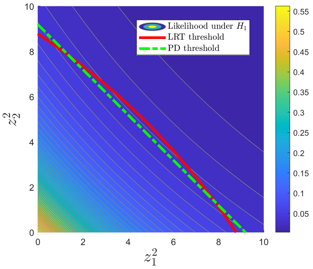
Here we consider scaling results for covert system performance under the block fading model with an arbitrary number of fading blocks per codeword in the absence of interference. Although the model is different than that considered in [4], a similar challenge arises: the performance of the optimal detector at Willie is not readily characterized. When faced with such a challenging characterization, authors often assume the adversary employs a reasonable but potentially sub-optimal detector such as a power detector, and then characterize covert system performance (e.g., [7, 8, 9, 10, 11, 12]). However, as illustrated in Section IV, the power detector differs from the optimal receiver in the presence of block fading, which underscores the need to specifically consider the optimal detector to investigate scaling laws of covert communication.

The work of [4] indicates that random jamming, the impairment considered there, has an asymmetric effect: it inhibits Willie’s ability to detect the signal more than Bob’s ability to decode it, hence improving covert throughput. Hence, in the case considered here, we might expect a similar effect: the block fading inhibits Willie’s ability to detect a transmission from Alice, and hence Alice should readily be able to match the AWGN case of [3] to use power ${\mathcal{O}}(1/\sqrt{n})$ and achieve throughput ${\mathcal{O}}(\sqrt{n})$; we make this rigorous with a convexity argument on the K-L distance in Theorem 1. Based on a similar line of reasoning, we might expect that the converse of [3] does not hold and that Alice might be able to transmit more than $O(\sqrt{n})$ bits. Perhaps surprisingly, we show that ${\mathcal{O}}(\sqrt{n})$ is still the upper bound.

The contributions of this work are:

  • We extend the analysis of [3] to environments with block fading with arbitrary block size. Our findings establish asymptotic bounds for covert communication taking into account these variable environmental factors, and throughout we consider the use of an optimal detector by the adversary.

  • We consider the scenario where the adversary, Willie, does not have prior knowledge of the distribution of the signal when Alice is transmitting. We demonstrate that our findings regarding the asymptotic limits and the effectiveness of the optimal detector remain valid even under this condition, thereby broadening the applicability of our results.

The paper is structured as follows. In Section 2, we define the problem and provide an overview of the covert communication system being studied. Section 3 presents the primary theoretical findings, encompassing the asymptotic bounds for the covertness. To validate the theoretical analysis, Section 4 offers an evaluation of system performance through numerical simulations. Finally, in Section 5, we conclude the paper by summarizing the key insights obtained.

II Problem Definition and Framework

II-A System Overview

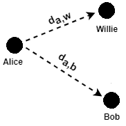
Figure 1 provides a schematic of the analyzed covert communication system. This includes Alice (a), who may attempt to send a message to her intended recipient, Bob (b), in such a way that it remains undetected by the observant adversary, Willie (w).

Refer to caption
Figure 1: Alice (a) is trying to send messages to Bob (b) without Willie (w) noticing. Here, $d_{x,y}$ stands for the distance from one transmitter $x$ to a receiver $y$.

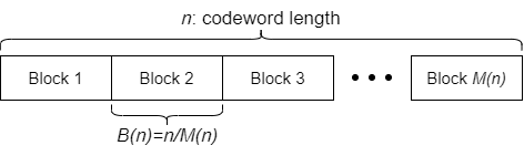
The framework for our study is grounded on the block fading model [13]. In this model, the length of a codeword, denoted as $n$, is divided into $M(n)$ separate fading blocks. This division is illustrated in Figure 2. Within each block, fading remains constant over its length $B(n)=n/M(n)$; however, the fading of different blocks of symbols is independent.

Refer to caption
Figure 2: Over the length of a codeword, denoted by $n$, signal fading occurs independently $M(n)$ times, resulting in a block of length $B(n)=n/M(n)$, within which the fading remains constant.

In each fading block $k$, the complex fading between a transmitter $x$ and a receiver $y$ is represented as $h_{k}^{(x,y)}$. In our context, $x$ is Alice (”$a$”), while $y$ is either Bob (”$b$”) or Willie (”$w$”). We assume Rayleigh fading, which implies that the complex fading coefficient $h_{k}^{(x,y)}$ is a zero-mean Gaussian random variable with $\mathbb{E}[|h_{x,y}|^{2}]=1$.

Alice decides whether to transmit ($H_{1}$) or to refrain from transmitting ($H_{0}$), with an equal chance of each of the two options. When Alice decides to transmit, her signal sequence is drawn from a codebook of the independent and identically distributed (i.i.d.) zero-mean Gaussian sequences $f_{1},f_{2},...,f_{n}$, with each symbol having a power of $P_{f}=\mathbb{E}[|f_{i}|^{2}]$.

For Willie, the received signal is then given as ($i=1,2,\ldots,n$):

$$Z_{i}=\begin{cases}\frac{h_{\lfloor i/B(n)\rfloor}^{(a,w)}f_{i}}{d_{a,w}^{\alpha/2}}+N_{i}^{(w)},&\text{if Alice transmits}\\ N_{i}^{(w)},&\text{if Alice doesn't}\end{cases}$$

where $\alpha$ represents the pathloss exponent, and $\{N_{i}^{(w)},i=1,2,...,n\}$ is a sequence of i.i.d. Gaussian random variables, each with zero mean and variance $\sigma_{w}^{2}$. Note that the power of the signal received from Alice then has an exponential distribution with mean $P_{f}/d_{aw}^{\alpha}$.

Similarly, for Bob, the received signal is modeled as:

$$Z_{i}=\begin{cases}\frac{h_{\lfloor i/B(n)\rfloor}^{(a,b)}f_{i}}{d_{a,b}^{\alpha/2}}+N_{i}^{(b)},&\text{if Alice transmits}\\ N_{i}^{(b)},&\text{if Alice doesn't}\end{cases}$$

where $\{N_{i}^{(b)},i=1,2,...,n\}$ is an i.i.d. sequence of Gaussian random variables, each with zero mean and variance $\sigma_{b}^{2}$.

From this model, it is worth noting that the block fading affecting the signal between Alice and Willie is an integral part of the communication setup.

II-B Covert Rate Asymptotics and Objectives

The central objective of this study is to derive asymptotic bounds on the number of bits that can be covertly transmitted in a given number of channel uses, in the presence of block fading between Alice and Willie. In the covert communication system, Willie, the adversary, performs a hypothesis test to determine if Alice transmitted in the slot of length $n$. Based on this, under hypothesis $H_{1}$, Alice has transmitted, while under hypothesis $H_{0}$, she has not.

Willie employs statistical hypothesis testing to distinguish between the null hypothesis and the alternative hypothesis. Willie’s goal is to minimize the probability of missed detection, $P_{MD}$, while ensuring a minimum false alarm rate, $P_{FA}$. These metrics provide a measure of the effectiveness of the covert communication system. The system is covert [3] if $P_{FA}+P_{MD}\geq 1-\epsilon$ for any $\epsilon>0$ when $n$ is sufficiently large.

III Main Results

We now present our results for the communication system under block fading conditions as described in the previous section. First, we present some foundational concepts related to covertness and hypothesis testing. Subsequently, we present the achievability and converse proofs.

III-A Preliminaries

Consider an i.i.d. sequence of real values $\{Z_{i}\}_{i=1}^{n}$ representing the signals received by Willie. We define two hypotheses:

  • Hypothesis $\mathrm{H_{0}}$: The distribution of observations under this hypothesis is represented as $\mathbb{P}_{0}$.

  • Hypothesis $\mathrm{H_{1}}$: The distribution under this hypothesis is denoted by $\mathbb{P}_{1}$.

Given that distribution $\mathbb{P}_{0}$ is known, Willie can formulate an optimal statistical hypothesis test (e.g., the Neyman-Pearson test given $\mathbb{P}_{1}$ is also known). This test minimizes the sum of error probabilities

$$\mathbb{P}_{E}=\mathbb{P}_{FA}+\mathbb{P}_{MD},$$

[14, Ch. 13]. In our analysis, we consider the cases that $\mathbb{P}_{1}$ is known or $\mathbb{P}_{1}$ is unknown.

For such a test scenario, the following theorem holds:

Theorem 1.

[3]

$$\mathbb{P}_{E}\geq 1-\sqrt{\frac{1}{2}{\mathcal{D}}(\mathbb{P}_{0}||\mathbb{P}_{1})}.$$

where ${\mathcal{D}}(\mathbb{P}_{0}||\mathbb{P}_{1})$ is the relative entropy, defined as follows.

Definition 1.

The relative entropy (also known as Kullback-Leibler divergence) between two probability measures $\mathbb{P}_{0}$ and $\mathbb{P}_{1}$ with corresponding nonnegative densities $f_{0}$ and $f_{1}$ is

$${\mathcal{D}}(\mathbb{P}_{0}||\mathbb{P}_{1})=\int_{0}^{\infty}f_{0}(x)\ln\frac{f_{0}(x)}{f_{1}(x)}dx.$$ (1)

Next, we present a theorem derived from the converse argument presented in [3]. This theorem is instrumental in the proof of the converse.

Theorem 2.

Let $\{X_{i}\}_{i=1}^{n}$ be a sequence of i.i.d. random variables. Consider two hypotheses $\mathrm{H_{0}}$ and $\mathrm{H_{1}}$. Suppose the following conditions are satisfied:

$\displaystyle-\infty<\mathbb{E}[X_{i}|\mathrm{H_{0}}]<\mathbb{E}[X_{i}|\mathrm{H_{1}}]$ $\displaystyle<\infty,$ (2)
$\displaystyle 0<\hbox{VAR}(X_{i}|\mathrm{H_{0}})$ $\displaystyle<\infty,$
$\displaystyle 0<\hbox{VAR}(X_{i}|\mathrm{H_{1}})$ $\displaystyle<\infty.$

If

$$\mathbb{E}[X_{i}|\mathrm{H_{1}}]-\mathbb{E}[X_{i}|\mathrm{H_{0}}]=\omega(1/\sqrt{n}),$$

then, $\{X_{i}\}_{i=1}^{n}$ under $\mathrm{H_{1}}$ can be readily distinguished from $\{X_{i}\}_{i=1}^{n}$ under $\mathrm{H_{0}}$, which means, as $n\to\infty$, $P_{MD}\to 0$ for any fixed $P_{FA}>0$.

III-B Achievability

Theorem 3 (Achievability).

Under the fading model introduced previously, given a total of $n$ channel uses, Alice can transmit $O(\sqrt{n})$ bits while remaining covert. This remains valid regardless of whether or not Willie knows $\mathbb{P}_{1}$.

Proof.

Let $\mathrm{Re}(z)$ and $\mathrm{Im}(z)$ denote the real and imaginary parts of $z\in\mathbb{C}$, respectively. Define

$$f(z,\theta)=f_{g}(\mathrm{Re}(z),\theta)f_{g}(\mathrm{Im}(z),\theta),$$ (3)

where

$$f_{g}(x,\theta)=\frac{1}{\sqrt{2\pi\theta}}e^{-\frac{x^{2}}{2\theta}},\quad x\in\mathbb{R}.$$

Define the realization of the random variables $Z_{i,1},Z_{i,2},\ldots,Z_{i,B(n)}$ as $\boldmath{z_{i}}=(z_{i,1},z_{i,2},\ldots,z_{i,B(n)})$. Let $\lambda=d_{aw}^{\alpha}$. Then, the probability density function of the $i$th block is

$\displaystyle\mathrm{H_{0}}:f_{0}(\boldmath{z_{i}})=\int_{0}^{\infty}\prod_{j=1}^{B(n)}f(z_{i,j},\sigma_{0}^{2})\lambda e^{-\lambda x}dx,$
$\displaystyle\mathrm{H_{1}}:f_{1}(\boldmath{z_{i}})=\int_{0}^{\infty}\prod_{j=1}^{B(n)}f(z_{i,j},\sigma_{0}^{2}+x\sigma_{a}^{2}(n))\lambda e^{-\lambda x}dx.$

The KL divergence is given by (1) which is not easily computed. However, invoking the convexity property of relative entropy [15] yields

$\displaystyle{\mathcal{D}}(f_{1}||f_{0})$
$\displaystyle\quad\leq\int_{-\infty}^{\infty}{\mathcal{D}}(f(z,\sigma_{0}^{2}+\sigma_{a}^{2}(n)x)^{B(n)}\|f(z,\sigma_{0}^{2})^{B(n)})\lambda e^{-\lambda x}dx.$

From this, using the additive property of relative entropy for independent distributions yields:

$\displaystyle{\mathcal{D}}(f_{1}||f_{0})$
$\displaystyle\quad\leq B(n)\int_{-\infty}^{\infty}{\mathcal{D}}(f(z,\sigma_{0}^{2}+\sigma_{a}^{2}(n)x)\|f(z,\sigma_{0}^{2}))\lambda e^{-\lambda x}dx.$

Following (3) and employing the same additive property,

$\displaystyle{\mathcal{D}}(f(z,\sigma_{0}^{2}+\sigma_{a}^{2}(n)x)\|f(z,\sigma_{0}^{2}))$
$\displaystyle\quad={\mathcal{D}}(f_{g}(\mathrm{Re}(z),\sigma_{0}^{2}+\sigma_{a}^{2}(n)x)\|f_{g}(\mathrm{Re}(z),\sigma_{0}^{2}))$
$\displaystyle\qquad+{\mathcal{D}}(f_{g}(\mathrm{Im}(z),\sigma_{0}^{2}+\sigma_{a}^{2}(n)x)\|f_{g}(\mathrm{Im}(z),\sigma_{0}^{2}))$
$\displaystyle\quad=2\times\big{(}-\frac{1}{2}\log(\frac{\sigma_{0}^{2}+x\sigma_{a}^{2}(n)}{\sigma_{0}^{2}})+\frac{\sigma_{0}^{2}+x\sigma_{a}^{2}(n)}{2\sigma_{0}^{2}}-\frac{1}{2}\big{)}$
$\displaystyle\quad=-\log\big{(}1+\frac{\sigma_{a}^{2}(n)}{\sigma_{0}^{2}}x\big{)}+\frac{\sigma_{a}^{2}(n)}{\sigma_{0}^{2}}x.$

This implies that

$\displaystyle{\mathcal{D}}(f_{1}||f_{0})$
$\displaystyle\quad\leq{B(n)}\int_{0}^{\infty}\big{(}-\log(1+\frac{\sigma_{a}^{2}(n)}{\sigma_{0}^{2}}x)+\frac{\sigma_{a}^{2}(n)}{\sigma_{0}^{2}}x\big{)}\lambda e^{-\lambda x}\,dx$
$\displaystyle\quad=-{B(n)}\int_{0}^{\infty}\log(1+\frac{\sigma_{a}^{2}(n)}{\sigma_{0}^{2}}x)\lambda e^{-\lambda x}\,dx+\frac{B(n)\sigma_{a}^{2}(n)}{\lambda\sigma_{0}^{2}}.$

We know that

$$\int_{0}^{\infty}\log(1+cx)\lambda e^{-\lambda x}\,dx=-e^{\lambda/c}\operatorname{Ei}(-\lambda/c),$$

where $\operatorname{Ei}(x)=-\int_{-x}^{\infty}\frac{e^{-t}}{t}\,dt$.

Therefore,

$\displaystyle{\mathcal{D}}(f_{1}||f_{0})$ $\displaystyle\leq{B(n)}e^{\frac{\lambda\sigma_{0}^{2}}{\sigma_{a}^{2}(n)}}\operatorname{Ei}\Big{(}-\frac{\lambda\sigma_{0}^{2}}{\sigma_{a}^{2}(n)}\Big{)}+\frac{B(n)\sigma_{a}^{2}(n)}{\lambda\sigma_{0}^{2}}.$

Since $\operatorname{Ei}(-x)<-\frac{1}{2}e^{-x}\log(1+\frac{2}{x})$ and $\log(1+x)\geq x-\frac{x^{2}}{2}$, we conclude

$\displaystyle{\mathcal{D}}(f_{1}||f_{0})$ $\displaystyle<-\frac{B(n)}{2}\log\Big{(}1+\frac{2}{\frac{\lambda\sigma_{0}^{2}}{\sigma_{a}^{2}(n)}}\Big{)}+\frac{B(n)\sigma_{a}^{2}(n)}{\lambda\sigma_{0}^{2}}$ (4)
$\displaystyle\leq-\frac{B(n)}{2}\Big{(}\frac{2}{\frac{\lambda\sigma_{0}^{2}}{\sigma_{a}^{2}(n)}}-\frac{1}{(\frac{\lambda\sigma_{0}^{2}}{\sigma_{a}^{2}(n)})^{2}}\Big{)}+\frac{B(n)\sigma_{a}^{2}(n)}{\lambda\sigma_{0}^{2}}$
$\displaystyle=\frac{B(n)\sigma_{a}^{4}(n)}{2\lambda^{2}\sigma_{0}^{4}}.$

From Theorem 1, it suffices to find the fastest growing $\sigma_{a}(n)$ such that

$$\lim_{n\rightarrow\infty}M(n){\mathcal{D}}(f_{0}||f_{1})<\infty,$$

which establishes

$$M(n)\frac{B(n)\sigma_{a}^{4}(n)}{2\lambda^{2}\sigma_{0}^{4}}={\mathcal{O}}(1).$$

This implies

$$\sigma_{a}^{2}(n)={\mathcal{O}}(1/\sqrt{M(n)B(n)})={\mathcal{O}}(1/\sqrt{n}).$$

This result is based on an optimal detector with knowledge of both $\mathbb{P}_{0}$ and $\mathbb{P}_{1}$. However, the validity of it persists even in scenarios where Willie is unaware of $\mathbb{P}_{1}$. This is attributed to the principle that Willie cannot surpass the scenario wherein complete knowledge is available. ∎

Theorem 3 confirms that Alice is able to transmit symbols at a power level of ${\mathcal{O}}(1/\sqrt{n})$ per symbol over a blocklength $n$, while ensuring covertness. It is important to note that the Alice-to-Bob communication channel is characterized as a block fading channel, which differs significantly from the AWGN channels typically assumed in reliable communication scenarios. Specifically, in block fading channels, there is some nonzero probability, not decreasing in $n$, that block fading will result in a received signal-to-interference-plus-noise ratio (SINR) that is insufficient for reliable communication [4].

III-C Converse

Theorem 4 (Converse).

Assume the fading model defined earlier with a total of $n$ symbols. In this case, there exists a detection method that restricts Alice’s covert symbol transmission to $O(\sqrt{n})$. This limitation holds whether or not Willie knows $\mathbb{P}_{1}$.

Proof.

Define rvs $Y_{i}=\sum_{j=1}^{B(n)}|Z_{i,j}|^{2}$, $i=1,2,\ldots$. Note that $\{Y_{i}\}_{i=1}^{n}$ are i.i.d.

In the case of $H_{0}$, we have

$\displaystyle\mathbb{E}_{0}[Y_{i}]$ $\displaystyle=B(n)\mathbb{E}[|Z_{i,j}|^{2}]$
$\displaystyle=2B(n)\sigma_{0}^{2}$

and similarly,

$\displaystyle\hbox{VAR}_{0}(Y_{i})$ $\displaystyle=B(n)\hbox{VAR}(|Z_{i,j}|^{2})$
$\displaystyle=4B(n)\sigma_{0}^{4}.$

Next, we calculate $\mathbb{E}_{1}[Y_{i}]$, and $\hbox{VAR}_{1}(Y_{i})$. Using the law of total expectation, we have

$\displaystyle\mathbb{E}_{1}[Y_{i}]$ $\displaystyle=\mathbb{E}_{X}[\mathbb{E}_{Y|X}[Y_{i}]]$
$\displaystyle=2B(n)\mathbb{E}_{X}[\sigma_{a}^{2}(n)X+\sigma_{0}^{2}].$

Given $X\sim\text{EXP}(\lambda)$, we have $\mathbb{E}[X]=\frac{1}{\lambda}$. Hence,

$\displaystyle\mathbb{E}_{1}[Y_{i}]$ $\displaystyle=2B(n)\big{(}\sigma_{0}^{2}+\frac{\sigma_{a}^{2}(n)}{\lambda}\big{)}.$

For the variance, using the properties of conditional variance,

$\displaystyle\hbox{VAR}_{1}(Y_{i})$ $\displaystyle=\hbox{VAR}_{X}(\mathbb{E}_{Y_{i}|X}[Y])+\mathbb{E}_{X}[\hbox{VAR}(Y|X)]$
$\displaystyle=\hbox{VAR}_{X}(2B(n)(\sigma_{a}^{2}(n)X+\sigma_{0}^{2}))$
$\displaystyle\quad+\mathbb{E}_{X}[2B(n)\times 2(\sigma_{a}^{2}(n)X+\sigma_{0}^{2})^{2}]$
$\displaystyle=4B(n)^{2}\sigma_{a}^{4}(n)\hbox{VAR}_{X}(X)$
$\displaystyle\quad+4B(n)\mathbb{E}_{X}[(\sigma_{a}^{2}(n)X+\sigma_{0}^{2})^{2}].$

Given $\mathbb{E}[X^{2}]=\frac{2}{\lambda^{2}}$ and $\hbox{VAR}[X]=\frac{1}{\lambda^{2}}$,

$\displaystyle\hbox{VAR}_{1}(Y_{i})$ $\displaystyle=4B(n)\Big{(}\sigma_{0}^{4}+\frac{2\sigma_{a}^{4}}{\lambda^{2}}+\frac{2\sigma_{a}^{2}(n)}{\lambda}\Big{)}+\frac{4B(n)^{2}\sigma_{a}^{4}}{\lambda^{2}}.$

Now, we use Theorem 2 to prove the converse for the fading model. Define the sequence

$$Y^{\prime}_{i}=\frac{1}{2\sqrt{B(n)}}Y_{i}-\sqrt{B(n)}\sigma_{0}^{2}$$

where $i=1,2,\ldots,M(n)$. We have

$$\mathbb{E}_{0}[Y^{\prime}_{i}]=0,\quad\hbox{VAR}_{0}(Y^{\prime}_{i})=\sigma_{0}^{4},\quad\mathbb{E}_{1}[Y^{\prime}_{i}]=\sqrt{B(n)}\frac{\sigma_{a}(n)^{2}}{\lambda},$$

and

$$\operatorname{VAR}_{1}(Y^{\prime}_{i})=\Big{(}\sigma_{0}^{4}+\frac{2\sigma_{a}(n)^{4}}{\lambda^{2}}+\frac{2\sigma_{a}(n)^{2}}{\lambda}\Big{)}+B(n)\frac{\sigma_{a}(n)^{4}}{\lambda^{2}},$$

which together with the assumption that $\sigma_{a}(n)^{2}=O(1/\sqrt{B(n)})$ implies that the conditions in (2) hold.

Suppose that $\sigma_{a}(n)^{2}=\omega(1/\sqrt{n})$. Then $\mathbb{E}_{0}[Y^{\prime}_{i}]=0$; hence,

$\displaystyle\mathbb{E}_{1}[Y^{\prime}_{i}]-\mathbb{E}_{0}[Y^{\prime}_{i}]$ $\displaystyle=\frac{\sqrt{B(n)}\sigma_{a}(n)^{2}}{\lambda}$
$\displaystyle=\sqrt{B(n)}\frac{\omega(1/\sqrt{n})}{\lambda}$
$\displaystyle=\omega\big{(}1/\sqrt{M(n)}\big{)}.$

From Theorem 2, this contradicts the covertness criterion. Since Theorem 2 assumes an adversary without knowledge of the distribution in the event of covert communication, we conclude that the converse results remain applicable when Willie is unaware of $\mathbb{P}_{1}$. ∎

IV Numerical Evaluation

Our aim is to validate the square root laws outlined in Section III, utilizing synthetic data. In what follows, we express Alice’s variance as $\sigma_{a}^{2}=c/n^{-\rho}$, $\rho\in(0,1)$. Figure 3 illustrates the error probability $P_{E}=P_{FA}+P_{MD}$ of Willie’s optimal detector, the Likelihood Ratio Test (LRT) as a function of $\rho$ for $\lambda=100$, $B(n)=1$, and four different values of $n$. The parameters are set as follows: $c=0.03$, and a false alarm probability $P_{FA}=0.01$.

As the value of $\rho$ increases, the error probability undergoes a noticeable transition, shifting from 0.01 to 1. This abrupt change is particularly evident at $\rho=0.5$, aligning with the condition $\sigma^{2}_{a}(n)=c/\sqrt{n}$. This observation is consistent with the square root law. We also observe that for the higher values of $n$, the phase transition is sharper.

Refer to caption
Figure 3: Phase transition analysis with $B(n)=1$, $\lambda=100$, $\sigma^{2}_{w}=1$, $P_{FA}=0.01$, and $\sigma^{2}_{a}=c/n^{-\rho}$ where $c=0.03$; as $\rho$ grows, $\sigma^{2}_{a}$ decreases and $P_{E}$ transitions from 0.01 to 1. This transition occurs around $\rho=0.5$, in agreement with the square root law.

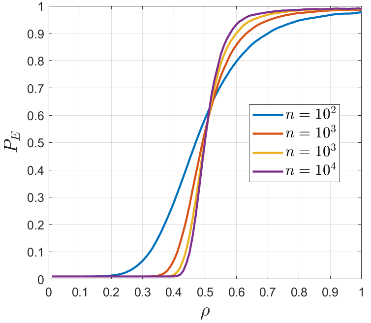
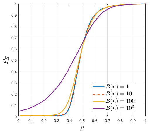
Figure 4 further explores the relationship between $P_{E}$ and $\rho$ by holding $n$ constant at $1000$ and varying the number of blocks, while maintaining the same parameters. This variation aims to assess the impact of block size on $P_{E}$ across three different block sizes. As the value of $\rho$ increases, the error probability shifts from 0.01 to 1. Again, this change is evident at $\rho=0.5$. Also, a smaller block size results in a sharper phase transition.

Refer to caption
Figure 4: Phase transition analysis with $n=1000$, $\lambda=100$, $\sigma^{2}_{w}=1$, $P_{FA}=0.01$, and $\sigma^{2}_{a}=c/n^{-\rho}$ where $c=0.03$. As $\rho$ increases, $\sigma^{2}_{a}$ decreases, leading to a transition in $P_{E}$ from 0.01 to 1. This transition is notably observed around $\rho=0.5$, aligning with the square root law.

Next, we explore whether the power detector (PD) is identical to the likelihood ratio test (LRT) or not. We consider a scenario with only two observations $z_{1}$ and $z_{2}$, akin to a demonstration by counterexample. We compare the power detector with the likelihood ratio test, denoted by $\Lambda(z_{1}^{2},z_{2}^{2})$. For the power detector to demonstrate optimality, its decision boundary, represented by the linear equation $z_{1}^{2}+z_{2}^{2}=\tau$ should ideally align with the contour where $\Lambda(z_{1}^{2},z_{2}^{2})=\tau^{\prime}$, where $\tau$ and $\tau^{\prime}$ are chosen such that $P_{FA}\leq 0.01$. However, as shown in Figure 5, this is not the case; instead of a straight line, $\Lambda(z_{1}^{2},z_{2}^{2})=\tau^{\prime}$ forms an arc. Hence, the power detector differs from the optimal test.

Refer to caption
Figure 5: Contour plot showing the function $\Lambda(z_{1}^{2},z_{2}^{2})=\tau^{\prime}$ where $\lambda=1$, $\sigma_{w}^{2}=1$, $\sigma_{a}^{2}=1$, and $\tau^{\prime}$ is chosen such that $P_{FA}\leq 0.01$. The arc-shaped contour demonstrates that a linear threshold test on powers, represented by $z_{1}^{2}+z_{2}^{2}=\tau$, where $\tau$ is chosen such that $P_{FA}\leq 0.01$, does not match the optimal test. For instance, when $z_{1}^{2}=z_{2}^{2}=4.8$, PD accepts $H_{1}$ (the hypothesis that there is covert communication between Alice and Bob) while the LRT rejects it. Conversely, when $z_{1}^{2}=9$ and $z_{2}^{2}=0.2$, PD rejects $H_{1}$ while the LRT accepts it.

V Conclusion

We examined the performance of covert communication systems in the presence of block fading, specifically focusing on the asymptotic laws for the number of bits that can be covertly transmitted. We established that the number of bits that can be transmitted covertly in $n$ channel uses is governed by ${\mathcal{O}}(\sqrt{n})$. To validate our theoretical findings, we conducted numerical simulations, which confirmed the trends observed in the theoretical analysis. By providing insights into the performance limitations imposed by fading, our research contributes to the advancement of covert communication systems, facilitating the design of more robust and efficient strategies for secure information transmission.

References

  • [1] M. Bloch, J. Barros, M. R. D. Rodrigues, and S. W. McLaughlin, “Wireless information-theoretic security,” IEEE Transactions on Information Theory, vol. 54, no. 6, pp. 2515–2534, 2008.
  • [2] Y. Liang, H. V. Poor, and S. Shamai, “Information theoretic security,” Foundations and Trends® in Communications and Information Theory, vol. 5, no. 4–5, pp. 355–580, 2009.
  • [3] B. A. Bash, D. Goeckel, and D. Towsley, “Limits of reliable communication with low probability of detection on awgn channels,” IEEE Journal on Selected Areas in Communications, vol. 31, no. 9, pp. 1921–1930, 2013.
  • [4] T. V. Sobers, B. A. Bash, S. Guha, D. Towsley, and D. Goeckel, “Covert communication in the presence of an uninformed jammer,” IEEE Transactions on Wireless Communications, vol. 16, no. 9, pp. 6193–6206, 2017.
  • [5] M. Tahmasbi, A. Savard, and M. R. Bloch, “Covert capacity of non-coherent rayleigh-fading channels,” IEEE Transactions on Information Theory, vol. 66, no. 4, pp. 1979–2005, 2019.
  • [6] D. Goeckel, A. Sheikholeslami, T. Sobers, B. A. Bash, O. Towsley, and S. Guha, “Covert communications in a dynamic interference environment,” in 2018 IEEE 19th International Workshop on Signal Processing Advances in Wireless Communications (SPAWC).   IEEE, 2018, pp. 1–5.
  • [7] T.-X. Zheng, H.-M. Wang, D. W. K. Ng, and J. Yuan, “Multi-antenna covert communications in random wireless networks,” IEEE Transactions on Wireless Communications, vol. 18, no. 3, pp. 1974–1987, 2019.
  • [8] A. Bendary, A. Abdelaziz, and C. E. Koksal, “Achieving positive covert capacity over mimo awgn channels,” IEEE Journal on Selected Areas in Information Theory, vol. 2, no. 1, pp. 149–162, 2021.
  • [9] L. Tao, W. Yang, S. Yan, D. Wu, X. Guan, and D. Chen, “Covert communication in downlink noma systems with random transmit power,” IEEE Wireless Communications Letters, vol. 9, no. 11, pp. 2000–2004, 2020.
  • [10] J. Hu, S. Yan, X. Zhou, F. Shu, and J. Wang, “Covert communications without channel state information at receiver in iot systems,” IEEE Internet of Things Journal, vol. 7, no. 11, pp. 11 103–11 114, 2020.
  • [11] X. Chen, W. Sun, C. Xing, N. Zhao, Y. Chen, F. R. Yu, and A. Nallanathan, “Multi-antenna covert communication via full-duplex jamming against a warden with uncertain locations,” IEEE Transactions on Wireless Communications, vol. 20, no. 8, pp. 5467–5480, 2021.
  • [12] X. Jiang, X. Chen, J. Tang, N. Zhao, X. Y. Zhang, D. Niyato, and K.-K. Wong, “Covert communication in uav-assisted air-ground networks,” IEEE Wireless Communications, vol. 28, no. 4, pp. 190–197, 2021.
  • [13] D. Tse and P. Viswanath, Fundamentals of wireless communication.   Cambridge university press, 2005.
  • [14] E. L. Lehmann, J. P. Romano, and G. Casella, Testing statistical hypotheses.   Springer, 2005, vol. 3.
  • [15] T. M. Cover and J. A. Thomas, Information theory and statistics, 2nd Ed.   John Wiley & Sons, Hoboken, NJ, 2002.