Sackin Indices for Labeled and Unlabeled Classes
of Galled Trees

Abstract

The Sackin index is an important measure for the balance of phylogenetic trees. We investigate two extensions of the Sackin index to the class of galled trees and two of its subclasses (simplex galled trees and normal galled trees) where we consider both labeled and unlabeled galled trees. In all cases, we show that the mean of the Sackin index for a network which is uniformly sampled from its class is asymptotic to $\mu n^{3/2}$ for an explicit constant $\mu$. In addition, we show that the scaled Sackin index convergences weakly and with all its moments to the Airy distribution.

AMS 2020 subject classifications. 05C20, 60C05, 60F05, 92D15.

Key words. Galled tree, Sackin index, asymptotic mean, limit law, Airy distribution.

1 Introduction and Results

Phylogenetic trees are used in evolutionary biology to model the ancestor relationship of a set of taxa ([26, 28]). In order to judge the suitability of a model, biologists have proposed many different shape parameters which measure how “balanced” a phylogenetic tree is; see the recent comprehensive survey [12]. One of the oldest of these balance parameters is the Sackin index which is defined as the sum of the root-to-leave distances over the set of all leaves. Statistical properties of the Sackin index have been obtained under several null models. For instance, for the uniform model or PDA model, where phylogenetic trees are uniformly sampled, the first-order asymptotics of the mean and variance have been found in [5]. Exact results for mean and variance are also known; see [9, 17, 22, 25]. In addition, the authors in [5] also showed that the scaled Sackin index converges to the Airy distribution. (Similar results were also proved for a closely related random variable, namely, the total path-length of Catalan trees; see, e.g., [11, 30].)

Despite the popularity of phylogenetic trees, they are often inappropriate as a model for evolution; see Chapter 10 in [28]. In particular, in the presence of reticulation events, phylogenetic trees need to be replaced by phylogenetic networks. We start with a precise definition of these objects.

Definition 1.

A (rooted, binary) phylogenetic network is an acyclic, directed graph with no multiple edges whose nodes fall into four categories:

• A unique root which is a node with indegree $0$ and outdegree $2$;

• Leaves which are nodes with indegree $1$ and outdegree $0$;

• Tree nodes which are nodes with indegree $1$ and outdegree $2$;

• Reticulation nodes which are nodes with indegree $2$ and outdegree $1$.

Remark 1.

Phylogenetic trees are phylogenetic networks without reticulation nodes.

The leaves of a phylogenetic network are usually labeled with the elements from a set $X$ of taxa (where each label is only used once). We then call the phylogenetic network labeled; otherwise, it is called unlabeled. Recent years have witnessed a growing body of work on enumeration and stochastic properties of shape parameters of the class of phylogenetic networks and its subclasses when networks are uniformly sampled from a given class; see, e.g., [6, 16, 18, 19, 24, 29]. However, very little is known about the extension of the Sackin index to networks.

First, we need to clarify what we mean by the Sackin index of a phylogenetic network. In fact, since there may be several paths from the root of the network to a given leave, different extensions of the Sackin index from trees to networks are possible. For instance, one can consider for every leaf the path of maximal length and sum these path lengths over all leaves. Alternatively, the path of minimal length can be considered. We investigate both these extensions in this paper and state a formal definition of the Sackin indices below. Other variants are conceivable, as for each gall (see below for the definition) that a path must go through, one has to decide which of the two possible ways to go. In the first extension (maximal length) one always chooses the longer one, in the second the shorter path is chosen. One may think of variants, e.g., choosing for each gall at random where to go.

The only stochastic result for a Sackin index of a phylogenetic network which we are aware of was obtained in [31] where the first extension above was considered for the class of one-component tree-child networks (called simplex networks in [31]). More precisely, it was proved that the mean of the Sackin index for a randomly chosen simplex tree-child networks with $n$ labeled leaves has the (unusual) order $n^{7/4}$; see [8] for a generalization of this result to $d$-combining simplex tree-child networks. No results for the variance and limit law of a Sackin index for networks have so far been reported in the literature.

The main purpose of this paper is to prove such results for the class of galled trees, which is a popular network class in phylogenetics; see [21, 27]. To define it, we need the notion of a tree-cycle (also called gall) which is a set of two edge disjoint paths from a tree node to a reticulation node with all intermediate nodes being also tree nodes.

Definition 2.

A phylogenetic network is called a galled tree if (i) every reticulation node is in a tree-cycle and (ii) any two tree-cycles are node-disjoint.

Remark 2.

Note that galled trees are not trees in the classical graph-theoretical sense. Nevertheless, we will refer to them as “trees” throughout this paper.

Galled trees with $n$ labeled leaves have been enumerated exactly in [27] and asymptotically in [6]. Moreover, exact enumeration results for the following two subclasses of labeled galled trees have been obtained in [7]. (For the first of these subclasses, a recursion relation and their asymptotic number in the unlabeled case were also recently obtained in [1].)

Definition 3.

A galled tree is called simplex (or one-component) if every reticulation node is followed by a leave. A galled tree is called normal if the parents of each reticulation node are not in an ancestor-descendant relationship.

Remark 3.

Simplex galled trees form an important building block in the construction of networks; see [7, 19]. Normal galled trees may be the most relevant galled trees in practical applications because they are exactly the rankable galled trees (i.e., , they can be generated by an evolution process); see [2].

We derive asymptotic counting results for these three classes (galled trees, simplex galled trees, and normal galled trees) in the next section (both for the labeled and unlabeled case). Our derivation will use the symbolic method as in [6] for labeled galled trees and will thus be different from the method used in [1] for unlabeled normal galled trees; in all other cases, the result will be new. However, our main focus in this paper is on moments and distributional results for the Sackin index which we formally define next. First, we need the notion of height for a leave.

network class	$(*,**)$	$\mu^{(*,**)}$
galled trees	$(\ell,\max)$	$\frac{47}{32}+\frac{39\sqrt{17}}{544}\approx 1.764340293\dots$
	$(\ell,\min)$	$\frac{49}{32}-\frac{7\sqrt{17}}{544}\approx 1.478195332\dots$
simplex galled trees	$(\ell,\max)$	$\sqrt{(2+\sqrt{2})/2}\approx 1.3065629648\dots$
	$(\ell,\min)$	$\sqrt{(2+\sqrt{2})/2}\approx 1.3065629648\dots$
normal galled trees	$(\ell,\max)$	$\approx 0.6434228878\dots$
	$(\ell,\min)$	$\approx 0.6062795760\dots$

Table 1: The mean constant for the different classes of galled trees and different Sackin indices in the labeled cases.

network class	$(*,**)$	$\mu^{(*,**)}$
galled trees	$(u,\max)$	$\approx 1.709905157\dots$
	$(u,\min)$	$\approx 1.4350664453\dots$
simplex galled trees	$(u,\max)$	$\approx 1.2514790858\dots$
	$(u,\min)$	$\approx 1.2514790858\dots$
normal galled trees	$(u,\max)$	$\approx 1.125542584\dots$
	$(u,\min)$	$\approx 1.0632588514\dots$

Table 2: The mean constant for the different classes of galled trees and different Sackin indices in the unlabeled cases.

Definition 4.

Let $N$ be a galled tree and $x$ be one of its leaves. Then the longer height $h^{+}(x)$ of $x$ is the length of a longest path from the root of $N$ to $x$. Likewise, we define analogously the shorter height $h^{-}(x)$ by the length of a shortest path from the root of $N$ to $x$.

Definition 5.

Let $N$ be a galled tree and $L$ be the set of all leaves of $N$. Then, depending on the choice of the height definition, we define the Sackin index of $N$ in two ways.

$$S^{+}(N):=\sum_{x\in L}h^{+}(x),\qquad S^{-}(N):=\sum_{x\in L}h^{-}(x).$$

We use throughout the work the notation $S_{n}^{(*,**)}$ where $*\in\{\ell,u\}$ (labeled and unlabeled) and $*\in\{\max,\min\}$ (maximal paths, minimal paths) to denote the Sackin indices of a random galled tree (or random simplex galled tree or random normal galled tree) with $n$ leaves, where random means that the galled tree is sampled uniformly at random from its class.

Our first main result concerns the mean of the Sackin indices.

Theorem 1.

For all cases, as $n\rightarrow\infty$,

$${\mathbb{E}}\left(S_{n}^{(*,**)}\right)\sim\sqrt{\pi}\mu^{(*,**)}n^{3/2},$$

where $\mu^{(*,**)}$ with $*\in\{\ell,u\}$ and $**\in\{\max,\min\}$ is given in Table 2 and Table 2.

Our second main result generalizes this to all higher moments and thus also gives a limiting distribution result for the Sackin indices.

Theorem 2.

In all cases, in distribution and with convergence of all moments, as $n\rightarrow\infty$,

$$\frac{S_{n}^{(*,**)}}{\mu^{(*,**)}}\stackrel{{\scriptstyle d}}{{\longrightarrow}}S,$$

where $S$ has the Airy distribution.

Remark 4.

The Airy distribution $S$ is the distribution which is uniquely determined by the following moment sequence:

$${\mathbb{E}}\left(S^{m}\right)=\frac{2\sqrt{\pi}}{\Gamma((3m-1)/2)}\Omega_{m},$$

where $\Gamma(x)$ is the gamma function and $\Omega_{m}$ is recursively given by $\Omega_{1}=1/2$ and

$$\Omega_{m}=\frac{m(3m-4)}{2}\Omega_{m-1}+\frac{1}{2}\sum_{\ell=1}^{m-1}\binom{m}{\ell}\Omega_{\ell}\Omega_{m-\ell},\qquad(m\geq 2).$$

Remark 5.

For the class of labeled galled trees, the convergence-in-distribution part of Theorem 2 is also a consequence of Theorem 1.2 in [29]. However, note that the scaling factor was not explicitly determined in [29].

We conclude the introduction with a brief sketch of the paper. In the next section, we recall the symbolic method and explain how it can be used for the enumeration of (labeled and unlabeled) galled trees. In Section 3, we derive the mean of both Sackin indices for labeled galled trees. These results are generalized to all moments in Section 4 which then also gives the limit law of the Sackin indices via the method of moments. In Section 5, we consider variants of the class of labeled galled trees. In Section 6, we derive similar results as in Section 3-5 for unlabeled galled trees. We conclude the paper with some remarks in Section 7.

2 Symbolic Method and Generating Functions

We will present what is needed of the symbolic method from analytic combinatorics. The method starts from combinatorial structures and uses constructions to build more complex objects. The power of the methods comes from a dictionary translating these constructions into algebraic operations on functions associated with the combinatorial structures, thus making the counting problems amenable to the huge arsenal of complex analysis. The primary source for this is [15], where many more constructions are presented along with numerous applications and more advanced methods.

2.1 Labeled structures and generating functions

We start with the basic definitions.

Definition 6.

A (labeled) combinatorial structure (often also called combinatorial class) is a pair $(\mathcal{A},|\cdot|)$, where $\mathcal{A}$ is a set of elements, called combinatorial objects, which are composed of distinguishable (i.e., labeled) atoms, and a size function $|\cdot|:\mathcal{A}\to\mathbb{N}$ such that for all $n\in{\mathbb{N}}$ the set $\mathcal{A}_{n}:=\{x\in\mathcal{A}\text{ such that }|x|=n\}$ is finite. The atoms of every object $x$ carry the labels $1,2\dots,|x|$.

The sequence $(a_{n})_{n\in\mathbb{N}}$ with $a_{n}=\#\mathcal{A}_{n}$, the cardinality of $\mathcal{A}_{n}$, is called the counting sequence of $\mathcal{A}$ and the formal power series $A(z)=\sum_{n\geq 0}a_{n}\frac{z^{n}}{n!}$ is the (exponential) generating function associated with $\mathcal{A}$.

Remark 6.

If the $(a_{n})_{n\in\mathbb{N}}$ does not grow too fast, then $A(z)$ has a positive radius of convergence and thus represents a function in some neighbourhood of the origin in ${\mathbb{C}}$.

The above mentioned dictionary translates combinatorial constructions (i.e., set operations involving the ground sets of combinatorial structures with compatible size functions) into algebraic operations on their generating functions. The concept is usually applied in the following way: Starting point is a combinatorial counting problem of the form ”‘How many objects of size $n$ are there in structure $\mathcal{A}$?”’ The next step is to find a specification for $\mathcal{A}$ using combinatorial constructions and known combinatorial structures. Finally, apply the dictionary and analyze the resulting generating functions.

Examples for combinatorial constructions

• Combinatorial sum: Given two combinatorial structures $(\mathcal{A},|\cdot|_{\mathcal{A}})$ and $(\mathcal{B},|\cdot|_{\mathcal{B}})$, let

  $$\mathcal{C}=\mathcal{A}~{}\dot{\cup}~{}\mathcal{B},\qquad|x|_{\mathcal{C}}=\begin{cases}|x|_{\mathcal{A}}&\text{ if }x\in\mathcal{A},\\ |x|_{\mathcal{B}}&\text{ if }x\in\mathcal{B},\end{cases}$$

  where $\dot{\cup}$ is the disjoint union. Thus, $C(z)=A(z)+B(z)$.

• Combinatorial product: Given two combinatorial structures $(\mathcal{A},|\cdot|_{\mathcal{A}})$ and $(\mathcal{B},|\cdot|_{\mathcal{B}})$ set

  $$\mathcal{C}=\mathcal{A}\times\mathcal{B},\qquad|(x,y)|_{\mathcal{C}}=|x|_{\mathcal{A}}+|y|_{\mathcal{B}}.$$

  Every atom of $x$ and every atom of $y$ becomes an atom of $(x,y)$ by this process. In order to get a correct labeling, relabel $x$ and $y$ in an order-preserving way such that the atoms of $(x,y)$ carry the labels $1,2,\dots,|x|+|y|$ after all. This relabeling is not unique, as we may choose which labels go into $x$, leaving the remaining labels for $y$. But as we do respect the order of the labels within $x$ and within $y$, each such choice results in a unique labeling of $(x,y)$. Altogether, we obtain

  $$c_{n}=\sum_{k=0}^{n}\binom{n}{k}a_{k}b_{n-k},$$

  as for $|(x,y)|=n$ the first component $x$ has size between 0 and $n$ and we have then $\binom{n}{k}$ possible choices for the labels of the atoms of $x$ inside $(x,y)$. This relation implies $C(z)=A(z)B(z).$

• Symmetric combinatorial product: Given a combinatorial structures $(\mathcal{A},|\cdot|_{\mathcal{A}})$, we may construct the combinatorial product $\mathcal{A}\times\mathcal{A}$, but identify $(x,y)$ and $(y,x)$. Here, we actually construct sets $\{x,y\}$ together with the combinatorial size function $|\{x,y\}|_{\mathcal{C}}=|x|_{\mathcal{A}}+|y|_{\mathcal{B}}$. For stressing the fact that we have a symmetry in the future formulas, let us write this as $\mathcal{C}=\mathcal{A}\ast\mathcal{A}$, although a more standard notation would be $\textsc{Set}_{2}(\mathcal{A})$.

  Note further, that in a pair $(x,y)$ we can never have $x=y$, as the objects are labeled. Thus, on the generating function level we get $D(z)=\frac{1}{2}A(z)^{2}$.

• Sequences of positive length: Let $(\mathcal{A},|\cdot|)$ be a combinatorial structure in which no object has size 0. The sequence construction we will use is defined by

  $$\mathcal{C}=\textsc{Seq}^{+}(\mathcal{A}):=\mathcal{A}~{}\dot{\cup}~{}(\mathcal{A}\times\mathcal{A})~{}\dot{\cup}~{}(\mathcal{A}\times\mathcal{A}\times\mathcal{A})~{}\dot{\cup}~{}\dots.$$

  Now, using the dictionary, we get

  $$C(z)=A(z)+A(z)^{2}+A(z)^{3}+\dots=\frac{A(z)}{1-A(z)}.$$

Remark 7.

In the standard literature the sequence construction has nonnegative length, i.e., the empty sequence is also allowed. As the empty sequence constitutes an object of size zero, we would just have to add 1 to the generating function $C(z)$, giving $C(z)=1/(1-A(z))$ after all. We chose to exclude the trivial object, as in all our specifications only positive length sequences will occur.

2.2 Unlabeled structures

Without being too formal, for unlabeled structures we simply dispense with the labeling of the atoms, which then become indistinguishable. Counting is then more complicated, as symmetries (non-trivial automorphisms) may occur. Nevertheless, for the basic structures that we discussed above for the labeled world, not much changes. Instead of exponential generating functions $A(z)=\sum_{n\geq 0}a_{n}\frac{z^{n}}{n!}$, we must use ordinary generating functions $A(z)=\sum_{n\geq 0}a_{n}z^{n}$. Then, we get the same relations for combinatorial sum, product and the sequence construction. In the symmetric combinatorial product, we must cope more carefully with symmetries, as the components of a pair $(x,y)$ need no longer be different. We will not develop the theory here and just state that the symmetric combinatorial product $\mathcal{A}=\mathcal{A}\ast\mathcal{A}$ has (ordinary) generating function $C(z)=(A(z)^{2}+A(z^{2}))/2$.

2.3 The generating function for galled trees

Let us apply the symbolic method to galled trees. We start with a symbolic equation, which is basically a context-free grammar that specifies galled trees.

Figure 1: Symbolic specification of galled trees.

A galled tree can be seen as an object that falls into one of four categories: The first one is a (labeled) leaf, the simplest possible galled tree. The second consists of a root being a tree vertex which has two children being galled trees. In this case there is a symmetry, as we may interchange the two children without changing the galled tree. The third category consists of galled trees with a root inside the gall. Additionally, we require that there is a nontrivial path from the root to the (unique) reticulation node of the gall and that the second ingoing edge of the reticulation node links the root directly to it. The vertices of the nontrivial path are tree nodes, and their second children are again galled trees. Likewise, the child of the reticulation node is a galled tree. The last category is similarly shaped, except that instead of the direct link from the root to the reticulation node there is a nontrivial path of tree nodes.

When regarding the set $\mathcal{R}$ of galled trees, then the symbolic specification above gives in a fairly straight-forward way a specification in terms of sets, the ground set of combinatorial structures.

$$\mathcal{R}=\{\Box\}~{}\dot{\cup}~{}\{\circ\}\times\left[(\mathcal{R}\ast\mathcal{R})~{}\dot{\cup}~{}\mathcal{R}\times\textsc{Seq}^{+}(\mathcal{R})~{}\dot{\cup}~{}\mathcal{R}\times(\textsc{Seq}^{+}(\mathcal{R})\ast\textsc{Seq}^{+}(\mathcal{R}))\right].$$ (1)

Now we use our dictionary. This yields a functional equation for the generating function associated with galled trees:

$$R(z)=z+\frac{1}{2}R(z)^{2}+\frac{R(z)^{2}}{1-R(z)}+\frac{1}{2}R(z)\left(\frac{R(z)}{1-R(z)}\right)^{2}.$$ (2)

This functional equation is a quartic equation for $R(z)$ and thus has four solutions. Note that $R(z)$ is a generating function, i.e., a power series with positive coefficients. Thus, it must be monotonically increasing and convex on the positive real line near the origin. Out of the four solutions only one satisfies all conditions. So, the desired generating function is

$$R(z)=\frac{5-\sqrt{1-8z}-\sqrt{18-8z-2\sqrt{1-8z}}}{4}=\sum_{n\geq 0}r_{n}\frac{z^{n}}{n!}$$

as has been already shown in [6].

2.4 Getting the coefficients

To solve the counting problem, we must compute the coefficients $[z^{n}]R(z)$ (notation for the $n$th coefficient of $R(z)$, i.e., , $r_{n}=n![z^{n}]R(z)$). The generating function is very explicit and could be expanded into a Taylor series. We will, however, extract the coefficients asymptotically. First, often the growth rate is displayed more explicitly by a simple asymptotic formula than with a complicated exact one. Second, for the study of the Sackin index, we will encounter more involved generating functions that only allow an asymptotic treatment, so we will need this technique anyway. This goes back to Flajolet and Odlyzko [14] and is also presented extensively in [15].

We start with the necessary definition.

Definition 7.

A function $f:\mathcal{D}\to{\mathbb{C}}$ with $\mathcal{D}\subseteq{\mathbb{C}}$ is called $\Delta$-analytic if there are $\eta>0$ and $0<\phi<\frac{\pi}{2}$ such that $f$ is analytic in $\Delta\setminus\{\rho\}$ where

$$\Delta=\Delta(\eta,\phi)=\{z\,\mid\;|z|\leq\rho+\eta,|\arg(z-\rho)|\geq\phi\}.\vspace*{-4mm}$$

Figure 2: The domain where we require analyticity.

Now, having a $\Delta$-analytic function that is singular at $\rho$, it turns out that the behaviour of the function near the singularity $\rho$ determines the behaviour of its coefficients. In this case, $\rho$ is the closest singularity to the origin. Such singularities (in principle, there maybe more, leading to more indentations of $\Delta$) are called dominant singularities. If there is more than one, each contributes to the coefficient asymptotics. Non-dominant singularities do contribute as well, but with smaller exponential order.

Theorem 3 (Transfer theorem [14]).

If $f(z)=\sum_{n}f_{n}z^{n}$ is $\Delta$-analytic and $f(z)\sim\left(1-\frac{z}{\rho}\right)^{\alpha}$ then

$$f_{n}\sim\rho^{-n}\frac{n^{-\alpha-1}}{\Gamma(-\alpha)}.$$

Remark 8.

An important aspect of this result is that it also applies to $f^{\prime}(z)$. (We will need this below.) More precisely, if $f(z)$ is $\Delta$-analytic and $f(z)\sim\left(1-\frac{z}{\rho}\right)^{\alpha}$, then $f^{\prime}(z)$ is also $\Delta$-analytic with $f^{\prime}(z)\sim-\frac{\alpha}{\rho}\left(1-\frac{z}{\rho}\right)^{\alpha-1}$ and thus

$$[z^{n}]f^{\prime}(z)\sim-\alpha\rho^{-n-1}\frac{n^{-\alpha}}{\Gamma(-\alpha+1)}=\rho^{-n-1}\frac{n^{-\alpha}}{\Gamma(-\alpha)};$$

see [14].

Our function $R(z)$ has a unique dominant singularity at $1/8$, where two of the three radicand vanish, and satisfies

$$R(z) =\frac{5-\sqrt{1-8z}-\sqrt{18-8z-2\sqrt{1-8z}}}{4}$$

$$\sim\frac{5-\sqrt{17}}{4}-\frac{17-\sqrt{17}}{68}\sqrt{1-8z},\quad\text{ as }z\to\frac{1}{8}.$$

Therefore, the above transfer theorem yields (as already computed in [6])

$$r_{n}\sim\frac{17-\sqrt{17}}{136}\cdot\frac{8^{n}n!}{\sqrt{\pi n^{3}}}\sim\frac{(17-\sqrt{17})\sqrt{2}}{136}\left(\frac{8}{e}\right)^{n}n^{n-1}.$$ (3)

3 The Mean of the Sackin Index in Galled Trees

First, let us fix $S^{+}$, the sum of the lengths of all maximal leaf-to-root paths in the network, as the variant of the Sackin index to be considered here. Thus, the induced random variable associated with networks with $n$ leaves is denoted by $S_{n}^{(\ell,\max)}$; see Table 2.

In order to study the Sackin index, we need to keep track of it using a second variable $x$ in the generating function. The variable $z$ keeps track of the size (number of leaves) of the galled trees. We obtain then a bivariate generating function

$$R(z,x)=\sum_{n\geq 0}\sum_{k\geq 0}r_{n,k}\frac{z^{n}}{n!}x^{k}$$

with $r_{n,k}$ being the number of galled trees with $n$ leaves and Sackin index equal to $k$. Given a uniform random network $N$ with $n$ leaves, then the expected Sackin index is

$$\mathbb{E}\left[S_{n}^{(\ell,\max)}\right]=\frac{\sum_{k\geq 0}kr_{n,k}}{r_{n}}=\frac{[z^{n}]R_{x}(z,1)}{[z^{n}]R(z)},$$

and hence expressible as an $n$th coefficient of a partial derivative of $R(z,x)$. So, the next task will be to find a suitable expression for $S(z):=R_{x}(z,1)$ and then extract the coefficients.

Note that the Sackin index is clearly additive: Indeed, we will see that when going through the cases listed on the right-hand side of the symbolic equation of Figure 1. The first case, where the network is a single leaf, is trivial. In the second case, each of the two occurrences of $\mathcal{R}$ contributes to the Sackin index of the galled tree. Its contribution is its own Sackin index with the number of its leaves added, as the height of a leaf in the galled tree is one more than its height in $\mathcal{R}$. The Sackin index of the galled tree is then the sum of the contributions of the two subtrees, after all. Likewise in the other cases: each $\mathcal{R}$ contributes its Sackin index and its number of leaves, multiplied by the height of the root of $\mathcal{R}$, as this is the value by which the leaf heights are lifted. Finally, all contributions are added.

By these additivity properties our dictionary translating the constructions presented in Section 2.1 into algebraic operations on generating function remains valid for bivariate generating functions as well. To cope with the modified leaf heights, note that a term $x^{n}z^{k}$ in the power series $R(z,x)$ represents a network with $n$ leaves and Sackin index $k$. If all leaf heights are increased by some number, say $m$, then the Sackin index becomes $k+nm$. The galled tree modified in this way now corresponds to $z^{n}x^{nm+k}=(zx^{m})^{n}x^{k}$. We see that in the end we only have to replace $z$ with $zx^{m}$, yielding $R(zx^{m},x)$. And note further that all we said so far in this section remains true if we replace $S^{+}$ with $S^{-}$.

These observations imply that the same specification as in the univariate case can be used, namely (1). And the modifications to the leaf heights caused by the combinatorial constructions are treated in a straight-forward way. We only have to introduce factors $x^{m}$ in a suitable way. This yields

$$R(z,x) =z+\frac{1}{2}R(zx,x)^{2}+\sum_{\ell\geq 0}\sum_{k>\ell}R(zx^{k+2},x)\prod_{i=1}^{k}R(zx^{i+1},x)\prod_{j=1}^{\ell}R(zx^{j+1},x)$$

$$\qquad+\frac{1}{2}\sum_{k\geq 1}R(zx^{k+2},x)\prod_{i=1}^{k}R(zx^{i+1},x)^{2}.$$ (4)

As mentioned above, we need $S(z):=R_{x}(z,1)$, so we now differentiate the functional equation above with respect to $x$ and set $x=1$. Note that $R_{z}(z,1)=R^{\prime}(z)$ and hence we obtain (omitting some tedious routine calculations that were done with MAPLE) $S(z)=zR^{\prime}(z)f(R(z))+g(R(z))S(z)$ implying

$$S(z)=\frac{zR^{\prime}(z)f(R(z))}{1-g(R(z))},$$

where

$$f(t) =\frac{t(2t^{5}-8t^{4}+10t^{3}-t^{2}-11t+12)}{(1-t)^{4}(1+t)},$$ (5)

$$g(t) =\frac{t(-2t^{3}+7t^{2}-9t+6)}{2(1-t)^{3}}.$$

As $S(z)$ depends only on $R(z)$ (via $f(t)$ and $g(t)$) and $1-g(R(z))\neq 0$ for $0\leq z<1/8$, there will be no pole in the denominator. Therefore, the dominant singularity of $S(z)$ is at $z=1/8$ as well. We can use the singular behaviour of $R(z)$ near $z=1/8$ to determine the behaviour of $S(z)$. Again, we omit tedious routine calculations and get

$$S(z)\sim\frac{95-\sqrt{17}}{544}\cdot\frac{1}{1-8z}\quad\text{ and so }\quad[z^{n}]S(z)\sim\frac{95-\sqrt{17}}{544}\cdot 8^{n},$$

and consequently, by (3), we get

$$\mathbb{E}\left[S_{n}^{(\ell,\max)}\right]=\frac{[z^{n}]S(z)}{[z^{n}]R(z)}\sim\left(\frac{47}{32}+\frac{39\sqrt{17}}{544}\right)\sqrt{\pi}n^{3/2}\approx 1.764340293\dots\cdot\sqrt{\pi}n^{3/2}.$$

If we look at $S^{-}$ instead of $S^{+}$, then the formal procedure is exactly the same with only a little modifications on the increments of the leaf height in the substructures. In fact, we have then

$$R(z,x) =z+\frac{1}{2}R(zx,x)^{2}+\sum_{\ell\geq 0}\sum_{k>\ell}R(zx^{\ell+2},x)\prod_{i=1}^{k}R(zx^{i+1},x)\prod_{j=1}^{\ell}R(zx^{j+1},x)$$

$$\qquad+\frac{1}{2}\sum_{k\geq 1}R(zx^{k+2},x)\prod_{i=1}^{k}R(zx^{i+1},x)^{2}.$$

Differentiating and setting $x=1$ gives this time

$$S(z)=\frac{zR^{\prime}(z)f(R(z))}{1-g(R(z))}$$

with

$$f(t) =\frac{t(2t^{5}-8t^{4}+10t^{3}-t^{2}-9t+10)}{(1-t)^{4}(1+t)},$$

$$g(t) =\frac{t(-2t^{3}+7t^{2}-9t+6)}{2(1-t)^{3}},$$

and so

$$S(z)\sim\frac{105-7\sqrt{17}}{544}\cdot\frac{1}{1-8z}\quad\text{ and so }\quad[z^{n}]S(z)\sim\frac{105-7\sqrt{17}}{544}\cdot 8^{n},$$

and this in conjunction with (3) yields

$$\mathbb{E}\left[S_{n}^{(\ell,\min)}\right]\sim\left(\frac{49}{32}-\frac{7\sqrt{17}}{544}\right)\sqrt{\pi}n^{3/2}\approx 1.478195332\dots\cdot\sqrt{\pi}n^{3/2}.$$

4 Limit Law of Sackin Indices

Our next goal is to find the limit law of the Sackin index of a uniform random galled tree with $n$ leaves, when $n$ tends to infinity. A weak limit theorem has been shown in [29], even in a more general setting. However, his result does not give explicit asymptotics of the moments. And in general, a weak limit does not even imply convergence of moments. In order to describe the limit law, we will compute the asymptotics of all moments and then apply the method of moments, showing that the limiting distribution is uniquely determined by its moments and implying a weak limit law as well.

We start with the functional equation (4),

$$R(z,x) =z+\frac{1}{2}R(zx,x)^{2}+\sum_{\ell\geq 0}\sum_{k>\ell}R(zx^{k+2},x)\prod_{i=1}^{k}R(zx^{i+1},x)\prod_{j=1}^{\ell}R(zx^{j+1},x)$$

$$\qquad+\frac{1}{2}\sum_{k\geq 1}R(zx^{k+2},x)\prod_{i=1}^{k}R(zx^{i+1},x)^{2},$$ (6)

and set

$$\Phi(z,A) =z+\frac{1}{2}A^{2}+\sum_{\ell\geq 0}\sum_{k>\ell}A^{\ell+k+1}+\frac{1}{2}\sum_{k\geq 1}A^{2k+1}$$

$$=z+\frac{1}{2}A^{2}+\frac{A^{2}}{(A-1)^{2}(A+1)}-\frac{A^{3}}{2(A^{2}-1)}.$$

This function captures the underlying structure of the functional equation: Indeed, if we replace all the $A$’s by $R(z,1)=R(z)$, we get with $A=\Phi(z,A)$ the functional equation (2) for $R(z)$.

Set $\rho=1/8$. Then, we know already that, as $z\to\rho$,

$$R(z,1)\sim\tau-a\sqrt{1-\frac{z}{\rho}}$$ (7)

with

$$\tau=\frac{5-\sqrt{17}}{4}\quad\text{ and }\quad~{}a=\frac{17-\sqrt{17}}{68}.$$

The $m$th factorial moment of $S_{n}^{(\ell,\max)}$ in a uniform random galled tree with $n$ leaves is related to $[z^{n}]R^{[m]}(z)$ where

$$R^{[m]}(z):=\frac{\partial^{m}}{\partial x^{m}}R(z,x)\biggr{\rvert}_{x=1}.$$

The $m$th moment is then a linear combination of all factorial moments up to order $m$. From the transfer theorem, Theorem 3, we know that the asymptotic growth of $R^{[m]}(z)$, when $z\to\rho$, and the growth of its coefficients are intimately related. Proposition 1 will yield asymptotics for $R^{[m]}(z)$ and as a consequence of this, we obtain that the $m$th factorial moments moments are asymptotically equal.

To get hands on $R^{[m]}(z)$, we need to do an $m$-fold differentiation on (6). This may look scary, but we only need the asymptotic main term of $R^{[m]}(z)$ which is given in the next proposition whose proof uses induction starting from (7) (and thus gives a second way of deriving the result of the previous section).

Proposition 1.

For $m\geq 1$,

$$R^{[m]}(z)\sim c_{m}\left(1-\frac{z}{\rho}\right)^{-(3m-1)/2},$$

where $c_{1}=f(\tau)/(2\Phi_{AA}(\rho,\tau))$, with $f$ from (5), and

$$c_{m}=\frac{f(\tau)}{2a\,\Phi_{AA}(\rho,\tau)}m(3m-4)c_{m-1}+\frac{1}{2a}\sum_{\ell=1}^{m-1}\binom{m}{\ell}c_{\ell}c_{m-\ell}$$ (8)

for $m\geq 2$.

Proof.

We differentiate the functional equation (6) $m$ times with respect to $x$ and set $x=1$. This gives

$$R^{[m]}(z)=G_{1}^{[m]}(z)+G_{2}^{[m]}(z)+G_{3}^{[m]}(z),$$ (9)

where

$$G_{1}^{[m]}(z) =\frac{1}{2}\sum_{i+j=m}\binom{m}{i}\frac{\partial^{i}}{\partial x^{i}}R(zx,x)\biggr{\rvert}_{x=1}\frac{\partial^{j}}{\partial x^{j}}R(zx,x)\biggr{\rvert}_{x=1},$$

$$G_{2}^{[m]}(z) =\sum_{\ell\geq 0}\sum_{k>\ell}\sum_{r_{1}+\cdots+r_{\ell+k+1}=m}\binom{m}{r_{1},\dots,r_{k+\ell+1}}\prod_{i=2}^{k+2}\frac{\partial^{r_{i-1}}}{\partial x^{r_{i-1}}}R(zx^{i},z)\biggr{\rvert}_{x=1}$$

$$\qquad\times\prod_{j=2}^{\ell+1}\frac{\partial^{r_{k+j}}}{\partial x^{r_{k+j}}}R(zx^{j},z)\biggr{\rvert}_{x=1},$$

$$G_{3}^{[m]}(z) =\frac{1}{2}\sum_{k\geq 1}\sum_{r_{1}+\cdots+r_{2k+1}=m}\binom{m}{r_{1},\dots,r_{2k+1}}\frac{\partial^{r_{1}}}{\partial x^{r_{1}}}R(zx^{k+2},x)\biggr{\rvert}_{x=1}$$

$$\qquad\times\prod_{i=2}^{k+1}\left(\frac{\partial^{r_{2i-2}}}{\partial x^{r_{2i-2}}}R(zx^{i}\!,z)\biggr{\rvert}_{x=1}\frac{\partial^{r_{2i-1}}}{\partial x^{r_{2i-1}}}R(zx^{i}\!,z)\biggr{\rvert}_{x=1}\right).$$

The right-hand side of (9) contains terms of the form $\frac{\partial^{m}}{\partial x^{m}}R(zx^{i},x)$, but by the multi-dimensional version of the Faà di Bruno formula (see e.g. [20]), we get

$$\frac{\partial^{m}}{\partial x^{m}}R(zx^{i},x)\biggr{\rvert}_{x=1}=R^{[m]}(z)+miz\frac{\partial}{\partial z}R^{[m-1]}(z)+\sum_{r_{1}=0}^{m-2}\sum_{r_{2}=1}^{m-r_{1}}K_{r_{1},r_{2}}(z)\frac{\partial^{r_{2}}}{\partial z^{r_{2}}}R^{[r_{1}]}(z),$$ (10)

where $K_{r_{1},r_{2}}(z)$ are polynomials in $z$ coming from inner derivatives. Their coefficients depend on $m$ and $i$.

Having this, we can now collect all occurrences of $R^{[m]}(z)$ on the right-hand side of (9), which yields $R^{[m]}(z)=\Phi_{A}(z,R(z))R^{[m]}(z)+H^{[m]}(z)$ after all. Solving for $R^{[m]}(z)$ gives

$$R^{[m]}(z)=\frac{H^{[m]}(z)}{1-\Phi_{A}(z,R(z))},$$ (11)

where $H^{[m]}(z)$ contains terms involving derivatives of $R^{[r]}(z)$ with $r<m$ and hence the induction hypothesis can be applied. The next goal is therefore to find the terms in $H^{[m]}(z)$ being asymptotically largest. Equivalently, we search for the terms of order $(1-\frac{z}{\rho})^{-\alpha}$ with largest $\alpha$.

To this end, note that according to the induction hypothesis, the $\alpha$ of $R^{[r]}(z)$ increases by $3/2$ when $r$ increases by one and increases by $1$ each time $R^{[r]}(z)$ is differentiated; see Remark 8. Thus, the largest $\alpha$ in $H^{[m]}(z)$ is obtained when using one of the two choices in the first sum of $G_{1}^{[m]}(z)$, $G_{2}^{[m]}(z)$, $G_{3}^{[m]}(z)$:

1. Either set all but one of the $m_{i}$’s equal to zero and pick the second term in the expansion (10) of the one term that is differentiated at least once,

2. or set all but exactly two of the $m_{i}$’s equal to zero and for both of the two corresponding terms pick the main term of their respective expansions (10).

Collecting all this gives

$$H^{[m]}(z)\sim d_{m}\left(1-\frac{z}{\rho}\right)^{-(3m-2)/2},$$

where $d_{1}=ab/2$ and for $m\geq 2$

$$d_{m}=b\frac{m(3m-4)}{2}c_{m-1}+\frac{\Phi_{AA}(\rho,\tau)}{2}\sum_{\ell=1}^{m-1}\binom{m}{\ell}c_{\ell}c_{m-\ell}$$

with

$$b =\tau+\sum_{\ell\geq 0}\sum_{k>\ell}\left(\binom{k+3}{2}+\binom{\ell+2}{2}-2\right)\tau^{k+\ell}$$

$$\qquad+\sum_{k\geq 1}\left(\frac{k+2}{2}+\binom{k+2}{2}-1\right)\tau^{2k}$$

$$=\frac{\tau(2\tau^{5}-8\tau^{4}+10\tau^{3}-\tau^{2}-11\tau+12)}{(1-\tau)^{4}(1+\tau)}=f(\tau).$$

So, we have so far

$$H^{[m]}(z)\sim d_{m}\left(1-\frac{z}{\rho}\right)^{-(3m-2)/2}\text{ and }\quad R^{[m]}(z)=\frac{H^{[m]}(z)}{1-\Phi_{A}(z,R(z))}.$$

Moreover, note that

$$\tau=\Phi(\rho,\tau)\quad\text{ and }\quad 1=\Phi_{A}(\rho,\tau).$$ (12)

Indeed, this is a consequence of the fact that $R(z)=\Phi(z,R(z))$, $\rho$ is a singular point of $R(z)$ and $R(\rho)=\tau$, and the implicit function theorem.

From (12), we get by Taylor’s theorem

$$1-\Phi_{A}(z,R(z))\sim a\,\Phi_{AA}(\rho,\tau)\sqrt{1-\frac{z}{\rho}},$$

and thus

$$R^{[m]}(z)\sim c_{m}\left(1-\frac{z}{\rho}\right)^{-(3m-1)/2}$$

with $c_{m}$ as claimed in (8).   

From the last result, we deduce our second main result; compare with Theorem 2.

Proposition 2.

Let $\mu:=f(\tau)/(a\,\Phi_{AA}(\rho,\tau))$. Then,

$$\frac{S_{n}^{(\ell,\max)}}{\mu n^{3/2}}\stackrel{{\scriptstyle d}}{{\longrightarrow}}S,$$

where the law of $S$ is the Airy distribution. In addition, all moments converge as well.

Proof.

Apply the transfer theorem, Theorem 3, to the result of Proposition 1. We get

$$\mathbb{E}\left[\left(\frac{S_{n}^{(\ell,\max)}}{\mu n^{3/2}}\right)^{m}\right]\sim\frac{1}{\mu^{m}n^{3m/2}}\frac{[z^{n}]R^{[m]}(z)}{[z^{n}]R(z)}\sim\frac{2\sqrt{\pi}}{\Gamma\left(\frac{3m-1}{2}\right)}\cdot\frac{c_{m}}{a\mu^{m}},$$

where the first asymptotic equivalence follows from the fact that the moments are asymptotic to the factorial moments (see above).

Set $\Omega_{m}:=c_{m}/(a\mu^{m})$. Then, the recurrence (8) for $c_{m}$ becomes

$$\Omega_{m}=\frac{m(3m-4)}{2}\Omega_{m-1}+\frac{1}{2}\sum_{\ell=1}^{m-1}\binom{m}{\ell}\Omega_{\ell}\Omega_{m-\ell}$$

and $\Omega_{1}=1/2$. Since

$$\frac{2\sqrt{\pi}\Omega_{m}}{\Gamma((3m-1)/2)}$$

are the moments of the Airy distribution (see [13]) and the Airy distribution is uniquely determined by its moments, the claimed result follows.   

Remark 9.

Using similar computations, we can show that the analogous result holds when $S_{n}^{(\ell,\max)}$ is replaced by $S_{n}^{(\ell,\min)}$.

5 Variations

In this section, we consider the two variants of galled trees introduced in the introduction (simplex galled networks and normal galled networks). Since only Theorem 1 is different for these two variants whereas Theorem 2 remains the same, we will focus on the former; the latter result is proved with the arguments from Section 4 with only minor modifications.

5.1 Simplex galled trees

Simplex galled trees, also called one-component galled trees are another model of galled trees studied in the literature. They differ slightly from galled trees by imposing the following constraint: The child of a reticulation node is always a leaf. So, adapting the specification of galled trees (Figure 1) is immediate; see Figure 3.

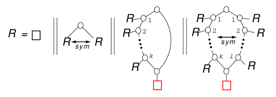
Figure 3: Symbolic equation for simplex galled trees. The red substructures are the places where galled trees and simplex galled trees differ.

The specification in terms of combinatorial structures and constructions is thus given by

$$\mathcal{R}=\{\Box\}~{}\dot{\cup}~{}\{\circ\}\times\left[(\mathcal{R}\ast\mathcal{R})~{}\dot{\cup}~{}\{\Box\}\times\textsc{Seq}^{+}(\mathcal{R})~{}\dot{\cup}~{}\{\Box\}\times(\textsc{Seq}^{+}(\mathcal{R})\ast\textsc{Seq}^{+}(\mathcal{R}))\right].$$ (13)

Using our dictionary, we obtain the functional equation for the generating function, which is

$$R(z)=z+\frac{1}{2}R(z)^{2}+\frac{zR(z)}{1-R(z)}+\frac{1}{2}z\left(\frac{R(z)}{1-R(z)}\right)^{2},$$ (14)

and admits the exact solution

$$R(z)=1-\frac{1}{2}\sqrt{2-2z+2\sqrt{1-6z+z^{2}}}$$

which is the unique power series solution.

It is easy to see that $R(z)$ is $\Delta$-analytic and has a unique dominant singularity at $\rho=3-2\sqrt{2}.$ Near $\rho$, we have the singular expansion

$$R(z)\sim 1-\sqrt{\sqrt{2}-1}-\frac{\sqrt{2-\sqrt{2}}}{2}\sqrt{1-\frac{z}{3-2\sqrt{2}}},\quad\text{ as }z\to\rho.$$ (15)

The transfer theorem gives therefore

$$\frac{r_{n}}{n!}=[z^{n}]R(z)\sim\frac{\sqrt{2-\sqrt{2}}}{4\sqrt{\pi n^{3}}}(3+2\sqrt{2})^{n}.$$

Note here that $3+2\sqrt{2}$ is the multiplicative inverse of $3-2\sqrt{2}$.

As in the case of galled trees, we use the specification from Figure 3 to derive a functional equation for the bivariate generating function. When writing (13) in the form

$$R(z) =z+\frac{1}{2}R(z)^{2}+\sum_{\ell\geq 0}\sum_{k>\ell}z\prod_{i=1}^{k}R(z)\prod_{j=1}^{\ell}R(z)+\frac{1}{2}\sum_{k\geq 1}z\prod_{i=1}^{k}R(z)^{2},$$

then each term $R(z)$ corresponds to one of the $\mathcal{R}$’s in (13), cf., also Figure 3. Therefore, each $R(z)$ must be replaced by a suitable $R(zx^{i+1},x)$. This gives

$$R(z,x) =z+\frac{1}{2}R(zx,x)^{2}+\sum_{\ell\geq 0}\sum_{k>\ell}zx^{k+2}\prod_{i=1}^{k}R(zx^{i+1},x)\prod_{j=1}^{\ell}R(zx^{j+1},x)$$

$$\qquad+\frac{1}{2}\sum_{k\geq 1}zx^{k+2}\prod_{i=1}^{k}R(zx^{i+1},x)^{2}.$$ (16)

Again, we set $S(z)=R_{x}(z,1)$ and derive the functional equation with respect to $x$ and set $x=1$. We get

$$S(z)=\frac{zR^{\prime}(z)f(z,R(z))+h(z,R(z))}{1-g(z,R(z))}$$ (17)

with

$$f(z,t)=t+z\frac{(2-t)}{(1-t)^{4}},\qquad g(z,t)=t+\frac{z}{(1-t)^{3}},\qquad h(z,t)=z\frac{t(2t^{3}-4t^{2}-t+6)}{2(1-t)^{3}(1+t)}.$$ (18)

From the singular behaviour of $R(z)$ and (17) we obtain

$$S(z)\sim\frac{1}{4}\frac{1}{1-(3+2\sqrt{2})z},\quad\text{ as }z\to 3-2\sqrt{2}.$$

This implies

$$\mathbb{E}\left[S_{n}^{(\ell,\max)}\right]\sim\frac{\sqrt{2+\sqrt{2}}}{\sqrt{2}}\sqrt{\pi}n^{3/2}\approx 1.306563\dots\cdot\sqrt{\pi}n^{3/2}.$$

The functional equation for the bivariate generating function for $S_{n}^{(\ell,\min)}$ is only slightly different from the one for $S_{n}^{(\ell,\max)}$. The only difference is in the double sum in (5.1), where the first factor $zx^{k+2}$ is changed to $zx^{\ell+2}$. Likewise, $S(z)$ can be expressed in term of $f(t)$, $g(t)$, and $h(t)$ (see (17)) with $f(t)$ and $g(t)$ as in (18) and in $h(t)$ only the constant 6 in the numerator is changed to 4. The asymptotics of $S(z)$ and hence for $\mathbb{E}\left[S_{n}^{(\ell,\min)}\right]$ does not change. Of course, this affects only the asymptotic main term. If we expand further to the next-order term, then we observe a difference. For displaying more details, let us write $S^{+}(z)$ and $S^{-}(z)$ for the generating functions of these two cases. And note that the second-order singular term of $R(z)$ is of order $(1-(3+2\sqrt{2})z)^{3/2}$. Hence, the term in the asymptotic expansion of $r_{n}$ is by a factor $n$ smaller than the main term, whereas it will turn out that the second-order terms of $[z^{n}]S^{+}(z)$ and $[z^{n}]S^{-}(z)$ are dominated by the main term only with a factor $\sqrt{n}$. Therefore, it suffices to expand $S^{+}(z)$ and $S^{-}(z)$, there is no need to look at further terms of $r_{n}$. Note, however, that for the further expansion of $S^{+}(z)$ and $S^{-}(z)$, (15) is not enough, i.e., we do need the next order term of $R(z)$. But as we have an explicit expression for $R(z)$, this is done automatically with MAPLE.

Expanding $S^{+}(z)$ and $S^{-}(z)$ up to their second-order terms gives

$$S^{+}(z) =\frac{1}{4}\frac{1}{1-(3+2\sqrt{2})z}+\frac{132+77\sqrt{2}+(4-36\sqrt{2})\sqrt{2\sqrt{2}-2}}{184}\frac{1}{\sqrt{1-(3+2\sqrt{2})z}}+{\mathcal{O}}\left(1\right),$$

$$S^{-}(z) =\frac{1}{4}\frac{1}{1-(3+2\sqrt{2})z}+\frac{52+15\sqrt{2}+(42-10\sqrt{2})\sqrt{2\sqrt{2}-2}}{184}\frac{1}{\sqrt{1-(3+2\sqrt{2})z}}+{\mathcal{O}}\left(1\right).$$

Using the transfer theorem then implies

$$\mathbb{E}\left[S_{n}^{(\ell,\max)}\right] =\frac{\sqrt{2+\sqrt{2}}}{2}\sqrt{\pi}n^{3/2}+\frac{132+77\sqrt{2}+(4-36\sqrt{2})\sqrt{2\sqrt{2}-2}}{46\sqrt{2-\sqrt{2}}}n+{\mathcal{O}}\left(\sqrt{n}\right)$$

$$\approx 1.306563\dots n^{3/2}+5.629479\dots\sqrt{n}+{\mathcal{O}}\left(1\right),$$

$$\mathbb{E}\left[S_{n}^{(\ell,\min)}\right] =\frac{\sqrt{2+\sqrt{2}}}{2}\sqrt{\pi}n^{3/2}+\frac{52+15\sqrt{2}+(42-10\sqrt{2})\sqrt{2\sqrt{2}-2}}{46\sqrt{2-\sqrt{2}}}n+{\mathcal{O}}\left(\sqrt{n}\right)$$

$$\approx 1.306563\dots n^{3/2}+2.799705\dots\sqrt{n}+{\mathcal{O}}\left(1\right).$$

5.2 Normal galled trees

Normal galled trees are exactly those galled trees that are rankable. Starting again from Figure 1, in the third case the parent nodes of the reticulation node are in an ancestor-descendant relationship, which is forbidden in normal networks. The other cases do not violate the normality condition. Therefore, we exclude the bad case and get the symbolic description shown in Figure 4.

Figure 4: Symbolic specification of normal galled trees.

This readily gives the specification in terms of combinatorial structures and constructions, namely,

$$\mathcal{R}=\{\Box\}~{}\dot{\cup}~{}\{\circ\}\times\left[(\mathcal{R}\ast\mathcal{R})~{}\dot{\cup}~{}\mathcal{R}\times(\textsc{Seq}^{+}(\mathcal{R})\ast\textsc{Seq}^{+}(\mathcal{R}))\right],$$ (19)

and our dictionary then yields the functional equation for the generating function:

$$R(z)=z+\frac{1}{2}R(z)^{2}+\frac{1}{2}R(z)\left(\frac{R(z)}{1-R(z)}\right)^{2}.$$

Out of the four solutions, exactly one is a power series with positive coefficients. This is

$$R(z)=\frac{3}{4}-\frac{\sqrt{3A}}{12}-\frac{1}{3}\cdot\sqrt{\frac{3\left(3\sqrt{3}B^{1/3}\left(\frac{17}{8}-z\right)-\left(\frac{B^{2/3}}{4}+\left(2z+\frac{13}{8}\right)B^{1/3}+z^{2}+2z+\frac{7}{4}\right)\sqrt{A}\right)}{B^{1/3}\sqrt{A}}},$$

where

$$A =\frac{4B^{2/3}-(16z+13)B^{1/3}+16z^{2}+32z+28}{B^{1/3}},$$

$$B =8z^{3}+24z^{2}-75z+44+3\sqrt{-192z^{4}-528z^{3}+645z^{2}-864z+177}.$$

As this is a very involved expression, we proceed by means of the implicit function theorem. Note that the pair $(\rho,\tau):=(\rho,R(\rho))$, where $\rho$ is the dominant singularity of $R(z)$, is the solution of the system

$$\tau =\rho+\frac{\tau^{2}}{2}+\frac{\tau}{2}\left(\frac{\tau}{1-\tau}\right)^{2},$$

$$1 =\tau+\frac{1}{2}\left(\frac{\tau}{1-\tau}\right)^{2}+\frac{\tau^{2}}{(1-\tau)^{3}}.$$ (20)

The second equation of this system is the derivative of the first one with respect to $\tau$. If we set

$$F(z,R)=-R+z+\frac{R^{2}}{2}+\frac{R}{2}\left(\frac{R}{1-R}\right)^{2},$$

then the system becomes $F(\rho,\tau)=0$, $F_{R}(\rho,\tau)=0$, which readily yields the singular points of $R(z)$. Expanding $F$ into a Taylor series around $(\rho,\tau)$ and using $F(z,R(z))=0$ as well as the fact that $(\rho,\tau)$ solves the system (5.2), we obtain that $R(z)-\tau={\mathcal{O}}\left(\sqrt{1-z/\rho}\right)$, and using this information in the Taylor expansion, the asymptotic relation

$$R(z)\sim\tau-\sqrt{\frac{2\rho F_{z}(\rho,\tau)}{F_{RR}(\rho,\tau)}}\sqrt{1-\frac{z}{\rho}},\text{ as }z\to\rho$$ (21)

is easily deduced. Expanding the Taylor series further, $R(z)$ could be asymptotically expanded to arbitrary order. These ideas are already found in [10]. From (5.2) even exact, however very involved, expressions for $\rho$ and $\tau$ can be found. We confine ourselves with the numerical approximations

$$\rho\approx 0.2382575749\dots\quad\text{ and }\quad\tau\approx 0.35829618282\dots.$$

Thus,

$$F_{z}(z,R)=1\quad\text{ and }\quad F_{RR}(z,R)=1+\frac{3R}{(1-R)^{4}},$$

and so $F_{RR}(\rho,\tau)\approx 7.3390612092\dots.$ This implies

$$\sqrt{\frac{2\rho F_{z}(\rho,\tau)}{F_{RR}(\rho,\tau)}}\approx 0.2548109584\dots,$$

from which we infer

$$\frac{r_{n}}{n!}=[z^{n}]R(z)\sim\frac{C_{R}}{\sqrt{\pi}n^{3/2}}\rho^{-n},\text{ with }C_{R}=\sqrt{\frac{\rho F_{z}(\rho,\tau)}{2F_{RR}(\rho,\tau)}}\approx 0.12740547924\dots$$ (22)

after all. Moreover, from (21) and Remark 8, we obtain

$$R^{\prime}(z)\sim\sqrt{\frac{F_{z}(\rho,\tau)}{2\rho F_{RR}(\rho,\tau)}}\frac{1}{\sqrt{1-\frac{z}{\rho}}},\text{ as }z\to\rho,\text{ where }\sqrt{\frac{F_{z}(\rho,\tau)}{2\rho F_{RR}(\rho,\tau)}}\approx 0.5347384202\dots.$$ (23)

For the bivariate function $R(z,x)$, we get, arguing as in the previous sections, the functional equation

$$R(z,x) =z+\frac{1}{2}R(zx,x)^{2}+\sum_{\ell\geq 1}\sum_{k>\ell}\prod_{i=1}^{k+1}R(zx^{i+1},x)\prod_{j=1}^{\ell}R(zx^{j+1},x)$$

$$\qquad+\frac{1}{2}\sum_{k\geq 1}R(zx^{k+2},x)\prod_{i=1}^{k}R(zx^{i+1},x)^{2}.$$ (24)

As before, set $S(z):=R_{x}(z,1)$ and differentiate the functional equation with respect to $x$ and let $x=1$ to get a linear equation for $S(z)$ having the solution

$$S(z)=\frac{zR^{\prime}(z)f(R(z))}{1-g(R(z))}$$

with

$$f(t)=\frac{t(2t^{5}-4t^{4}-2t^{3}+5t^{2}+t+2))}{2(1+t)^{3}(1-t)^{4}}\quad\text{ and }\quad g(t)=\frac{t(2t^{3}-5t^{2}+3t-2)}{2(1-t)^{3}}.$$

By means of (21) and (23), the singularity expansion of $S(z)$ is given by

$$S(z)\sim\frac{\rho R^{\prime}(\rho)s(\tau)}{1-\frac{z}{\rho}},\text{ as }z\to\rho$$

with

$$s(t)=\frac{t\left(2t^{5}-4t^{4}-2t^{3}+5t^{2}+t+2\right)}{2(1+t)^{3}(1-t)^{4}{\displaystyle\left(\frac{6C_{R}}{1-t}-\frac{t(6C_{R}t^{2}-10C_{R}t+3C_{R})}{(1-t)3}+\frac{2C_{R}}{t}\right)}}.$$

Numerically, we get $C_{S}:=\rho R^{\prime}(\rho)s(\tau)\approx 0.0819756013\dots$, and so we get finally $[z^{n}]S(z)\sim C_{S}\rho^{-n}$. This in conjunction with (22) eventually gives

$$\mathbb{E}\left[S_{n}^{(\ell,\max)}\right]\sim C^{+}\sqrt{\pi}n^{3/2}\quad\text{ with }\quad C^{+}=\frac{C_{S}}{C_{R}}\approx 0.6434228878\dots.$$

Turning to $S_{n}^{(\ell,\min)}$, in the functional equation (24), we have to change range of the two products in the double sum: Instead of $\prod_{i=1}^{k+1}\dots\prod_{j=1}^{\ell}\dots$, we must have $\prod_{i=1}^{k}\dots\prod_{j=1}^{\ell+1}\dots$, which is the only change. Similar computations as before yield then

$$\mathbb{E}\left[S_{n}^{(\ell,\min)}\right]\sim C^{-}\sqrt{\pi}n^{3/2}\quad\text{ with }\quad C^{-}\approx 0.6062795760\dots.$$

6 Unlabeled Galled Trees

For the unlabelled counterparts of the considered leaf-labeled classes of galled trees, we again only consider the derivation of the asymptotics of the mean (Theorem 1), in particular, the computation of the multplicative constants; the limit law (Theorem 2) again follows with similar tools as in Section 4 (only minor modifications are needed).

We use the same specifications (1), (13), and (19), respectively. The only difference lies in the dictionary that is used to translate this into functional equations for the generating functions, and within there only the treatment of the symmetric combinatorial product differs from the labeled cases. In the following subsections, we will briefly sketch how to deal with unlabeled classes.

6.1 General case

In the general case, we deal with unlabeled galled trees without any further constraint. They are described in Figure 1 and specified by (1). Using the translation scheme for unlabeled structures, this leads to the functional equation

$$R(z)=z+\frac{R(z)^{2}+R(z^{2})}{2}+\frac{R(z)^{2}}{1-R(z)}+\frac{R(z)}{2}\left(\left(\frac{R(z)}{1-R(z)}\right)^{2}+\frac{R(z^{2})}{1-R(z^{2})}\right).$$ (25)

Due to the terms involving $z^{2}$, it is impossible to derive an explicit formula for $R(z)$. We will, however, again appeal to the implicit function theorem to get the dominant singularity $\rho$ and $\tau=R(\rho)$. Setting $\sigma=R(\rho^{2})$, then we have (taking (25) at $z=\rho$ and its derivative with respect to $\tau$)

$$\tau =\rho+\frac{\tau^{2}+\sigma}{2}+\frac{\tau^{2}}{1-\tau}+\frac{\tau}{2}\left(\left(\frac{\tau}{1-\tau}\right)^{2}+\frac{\sigma}{1-\sigma}\right),$$

$$1 =\tau+\frac{2\tau-\tau^{2}}{(1-\tau)^{2}}+\frac{3\tau^{2}-\tau^{3}}{(1-\tau)^{3}}+\frac{1}{2}\frac{\sigma}{1-\sigma}.$$

Note further that, if we write (25) as $R(z)=\Psi(R(z))$, then $\Psi$ is an operator on the set of formal power series that is a contraction with respect to the formal topology (cf., [15, Appendix A]. If we start from the null series and iterate $\Psi$, then the iterate $\Psi^{m}(0)$ is a power series that coincides in its first $m$ terms with $R(z)$. As $\rho<1$, for $0<z<\rho$, we have $z^{2}<z$. This implies that $R(z^{2})$ converges very fast, which enables us to get accurate approximations of $\sigma=R(\rho^{2})$. Using this value, the system above can be solved numerically for $\rho$ and $\tau$. We get

$$\rho\approx 0.1164742652\dots\quad\text{ and }\quad\tau\approx 0.2182060577\dots,$$

and also $\sigma\approx 0.0139559001\dots$.

Remark 10.

Caveat: Approximating $\tau$ by solving for $\rho$ and inserting into $R(z)$ would be very inefficient, as $R(z)$ converges very slowly at $z=\rho$. Indeed, the convergence rate is only $\Theta(1/\sqrt{n})$ if $n$ terms of the power series are used.

As in the labeled cases, expanding the functional equation $F(z,R(z))=0$ at the singularity gives the singular expansion (21), where $F$ is given by

$$F(z,R)=-R+z+\frac{R^{2}+\sigma}{2}+\frac{R^{2}}{1-R}+\frac{R}{2}\left(\left(\frac{R}{1-R}\right)^{2}+\frac{\sigma}{1-\sigma}\right).$$

Taking partial derivatives gives

$$F_{RR}(z,R) =\frac{R^{4}-4R^{3}+6R^{2}-3R+3}{(1-R)^{4}},$$

$$F_{z}(z,R) =1+zR^{\prime}(z^{2})+\frac{zR^{\prime}(z^{2})R}{1-R(z^{2})},$$

and so we obtain

$$R(z)\sim\tau-C\sqrt{1-\frac{z}{\rho}}\quad\text{ where }\;C\approx 0.196590883\dots.$$

This implies

$$\frac{r_{n}}{n!}=[z^{n}]R(z)\sim\frac{C_{R}}{\sqrt{\pi n^{3}}}\rho^{-n}\quad\text{with}\quad C_{R}=C/2.$$

Now, let us turn to the Sackin index. Like in the labeled cases, we obtain from (25) the functional equation for $S(z)=R_{x}(z,x)$, with $x$ keeping track of the value of the Sackin index. By the additivity of the Sackin index, the treatment of the symmetric combinatorial product for the multivariate function $R(z,x)$ is like for $R(z)$. For $R(z,x)$, we get

$$R(z,x)=z +\frac{R(zx,x)^{2}+R(z^{2}x^{2},x^{2})}{2}+\sum_{\ell\geq 0}\sum_{k>\ell}\prod_{i=1}^{k+1}R(zx^{i+1},x)\prod_{j=1}^{\ell}R(zx^{j+1},x)$$

$$+\frac{1}{2}\sum_{k\geq 1}R(zx^{k+2},x)\left(\prod_{i=1}^{k}R(zx^{i+1},x)^{2}+\prod_{i=1}^{k}R(z^{2}x^{2i+2},x^{2})\right),$$

and for $S(z)$ this implies

$$S(z)=\frac{zR^{\prime}(z)f(z,R(z))+h(z,R(z))}{1-g(z,R(z))}$$

with

$$f(z,t) =\frac{2t^{5}-8t^{4}+10t^{3}-t^{2}-11t+12}{2(1+t)^{3}(1-t)^{4}}+\frac{R(z^{2})(3-2R(z^{2}))}{2(1-R(z^{2}))^{2}},$$

$$g(z,t) =\frac{t(-2t^{3}+7t^{2}-9t+6)}{2(1-t)^{3}}+\frac{R(z^{2})}{2(1-R(z^{2}))},$$

$$h(z,t) =z^{2}R^{\prime}(z^{2})\left(1+\frac{t(2-R(z^{2}))}{(1-R(z^{2}))^{3}}\right)+S(z^{2})\left(1+\frac{t}{(1-R(z^{2}))^{2}}\right).$$

The next step is to determine the singular expansion of $S(z)$, namely,

$$S(z)\sim\frac{C_{S}}{1-\frac{z}{\rho}},\quad\text{ as }z\to\rho,$$

Luckily enough, the nasty terms $S(z^{2})$ and $R^{\prime}(z^{2})$, which would require a cumbersome numerical treatment do not show up in the main coefficient $C_{S}$ which happens to depend only on $\rho$, $\tau$, $\sigma$, and $C$. So, we easily compute that $C_{S}\approx 0.168075882\dots$ and obtain finally

$$\mathbb{E}\left[S_{n}^{(u,\max)}\right]\sim C^{+}\sqrt{\pi}n^{3/2}\quad\text{ with }\quad C^{+}=\frac{C_{S}}{C_{R}}\approx 1.7099051570\dots,$$

and in a similar way for the other variant of the Sackin index:

$$\mathbb{E}\left[S_{n}^{(u,\min)}\right]\sim C^{-}\sqrt{\pi}n^{3/2}\quad\text{ with }\quad C^{-}\approx 1.4350664453\dots.$$

6.2 Simplex galled trees

As before, we start from the generic specification (13) but take the unlabeled translation scheme instead. We obtain

$$R(z)=z+\frac{R(z)^{2}+R(z^{2})}{2}+\frac{zR(z)}{1-R(z)}+\frac{z}{2}\left(\left(\frac{R(z)}{1-R(z)}\right)^{2}+\frac{R(z^{2})}{1-R(z^{2})}\right).$$

Like in the general case, we are faced with a functional equation of the form $R(z)=\Psi(R(z))$ with $\Psi$ being a contraction on the set of formal power series. Again, $R(\rho^{2})$ converges rapidly and so the corresponding system for $(\rho,\tau=R(\rho))$ can be easily solved numerically. This gives

$$\rho=0.162165279\dots\quad\text{ and }\quad\tau=0.365415487\dots.$$

This allows the numerical computation of the singular expansion (21) of $R(z)$, thus giving us hands on the asymptotics of its coefficients. Here, the multiplicative scaling factor of the singular term in $R(z)\sim\tau-C\sqrt{1-\frac{z}{\rho}}$ is $C\approx 0.3995272519\dots$, which gives the coefficient asymptotics $[z^{n}]R(z)\sim\left(C_{R}/\sqrt{\pi n^{3}}\right)\rho^{-n}$ with $C_{R}=C/2$.

Likewise, the bivariate problem is treated as in the previous section. The functional equation for $R(z,x)$ reads as

$$R(z,x=z +\frac{R(zx,x)^{2}+R(z^{2}x^{2},x^{2})}{2}+\sum_{\ell\geq 0}\sum_{k>\ell}zx^{k+2}\prod_{i=1}^{k}R(zx^{i+1},x)\prod_{j=1}^{\ell}R(zx^{j+1},x)$$

$$+\frac{1}{2}\sum_{k\geq 1}zx^{k+2}\left(\prod_{i=1}^{k}R(zx^{i+1},x)^{2}+\prod_{i=1}^{k}R(z^{2}x^{2i+2},x^{2})\right),$$ (26)

implying

$$S(z)=\frac{zR^{\prime}(z)f(z,R(z))+h(z,R(z))}{1-g(z,R(z))}$$ (27)

with

$$f(z,t)=t+z\frac{2-t}{(1-t)^{4}},\qquad g(z,t)=t+\frac{z}{(1-t)^{3}},$$

and

$$h(z,t) =z^{2}R^{\prime}(z^{2})\left(1+\frac{z(2-R(z^{2}))}{(1-R(z^{2}))^{3}}\right)+S(z^{2})\left(1+\frac{z}{(1-R(z^{2}))^{2}}\right)$$

$$\quad+z\frac{3R(z^{2})-2R(z^{2})^{2}}{(1-R(z^{2}))^{2}}+z\frac{t(t^{3}-4t^{2}-t+6)}{2(1-t)^{3}(1+t)}.$$ (28)

Now use the singular expansion of $R(z)$ at $\rho$ to obtain that $S(z)\sim C_{S}\left(1-\frac{z}{\rho}\right)^{-1}$, as $z\to\rho$, where $C_{S}=1/4$. Eventually, this gives

$$\mathbb{E}\left[S_{n}^{(u,\max)}\right]\sim C^{+}\sqrt{\pi}n^{3/2}\quad\text{ with }\quad C^{+}=\frac{C_{S}}{C_{R}}\approx 1.2514790858\dots,$$

and similarly

$$\mathbb{E}\left[S_{n}^{(u,\min)}\right]\sim C^{-}\sqrt{\pi}n^{3/2}\quad\text{ with }\quad C^{-}=C^{+}.$$

As in the labeled case for simplex trees, we encounter here the phenomenon that the two variants of the Sackin index are asympotically the same. Their difference shows only up in the second-order term of the asymptotics.

This time, we do not have an explicit expression for $R(z)$ that can be expanded, as in the labeled case. So, we need to go back to the functional equation and expand $F(z,R)$ further into a Taylor series at $(\rho,\tau)$, noting that $F(z,R(z))=0$, $F_{R}(\rho,\tau)=0$ and that $R(z)-\tau\sim-C\sqrt{z-\rho}$, as $z$ approaches $\rho$, where $C=\sqrt{\rho F_{z}(\rho,\tau)/F_{RR}(\rho,\tau)}$, cf. (21). This yields, as $z\to\rho$,

$$0=F_{z}(z-\rho)+\frac{F_{RR}}{2}(R-\tau)^{2}+F_{zR}(z-\rho)(R-\tau)+\frac{F_{RRR}}{6}(R-\tau)^{3}+{\mathcal{O}}\left(|z-\rho|^{2}\right),$$

where the partial derivatives of $F$ are evaluated at $(\rho,\tau)$. Consequently,

$$R(z) \sim\tau-C\sqrt{1-\frac{z}{\rho}}\sqrt{1+C\cdot\left(\frac{F_{RRR}}{3F_{RR}}-\frac{F_{zR}}{F_{z}}\right)}$$

$$\sim\tau-C\sqrt{1-\frac{z}{\rho}}-\frac{C^{2}}{2}\left(\frac{F_{RRR}}{3F_{RR}}-\frac{F_{zR}}{F_{z}}\right)\left(1-\frac{z}{\rho}\right)$$

$$=\tau-C\sqrt{1-\frac{z}{\rho}}+D\left(1-\frac{z}{\rho}\right)$$

with $D\approx 0.0520951948$, which implies, by Remark 8,

$$R^{\prime}(z)\sim\frac{C}{2\rho}\left(1-\frac{z}{\rho}\right)^{-1/2}-\frac{D}{\rho}.$$

This enables us to obtain the second-order term in the singular expansions of $f(z,R(z))$ and $g(z,R(z))$:

$$f(z,R(z))\sim 2+D_{f}\sqrt{1-\frac{z}{\rho}}\text{ and }1-g(z,R(z))\sim C_{g}\sqrt{1-\frac{z}{\rho}}+D_{g}\left(1-\frac{z}{\rho}\right)$$

with $D_{f}\approx-4.1164638932\dots$, $C_{g}\approx 1.5981090076\dots$ and $D_{g}\approx-1.5092271101\dots$. From (27), we get then

$$S(z)\sim\frac{C_{S}}{1-\frac{z}{\rho}}+\frac{CD_{f}C_{g}-2DC_{f}C_{g}-CC_{f}D_{g}+2C_{g}H}{2C_{g}^{2}}\frac{1}{\sqrt{1-\frac{z}{\rho}}},$$

where $H=\lim_{z\to\rho}h(z,R(z))$. The computation of $H$ requires to determine $S(\rho^{2})$.

One way to do this is appealing to the functional equation (26) and using the fact that the right-hand side can be seen the application of an operator to $R(z,x)$ that is a contraction in the formal metric. The convergence is exponential, so not many coefficients are needed, but as the coefficient $z^{n}$ is a polynomial in $x$ and we get only one additional correct coefficient per iteration, this requires heavy computations.

Alternatively, we may use (27). Iterating this means that we actually insert values $z^{2^{i}}$ into the functions, which proves very efficient. We obtain $S(\rho^{2})\approx 0.0059339813\dots$, and can therefore compute $H$. Here also lies the only difference between the two Sackin indices. Computing $H$ for both cases gives the desired result after all:

$$S^{\pm}(z)\sim\frac{C_{S}}{1-\frac{z}{\rho}}+\frac{D_{S}^{\pm}}{\sqrt{1-\frac{z}{\rho}}}$$

with $D_{S}^{+}\approx-0.033882959\dots$ and $D_{S}^{-}\approx-0.140151617\dots$, which leads to the final result

$$\mathbb{E}\left[S_{n}^{(u,\max)}\right] \sim K\sqrt{\pi}n^{3/2}+\frac{C_{R}}{D_{S}^{+}}n,$$

$$\mathbb{E}\left[S_{n}^{(u,\min)}\right] \sim K\sqrt{\pi}n^{3/2}+\frac{C_{R}}{D_{S}^{-}}n,$$

where $K=C^{+}=C^{-}$ and $C_{R}/D_{S}^{+}\approx-0.1696152609\dots$ and $C_{R}/D_{S}^{-}\approx-0.701587271\dots$.

6.3 Normal galled trees

In the case of normal galled trees, we play the same game again. In the specification (19) as before, we get the functional equation

$$R(z)=z+\frac{R(z)^{2}+R(z^{2})}{2}+\frac{R(z)}{2}\left(\left(\frac{R(z)}{1-R(z)}\right)^{2}+\frac{R(z^{2})}{1-R(z^{2})}\right).$$

From this, we obtain in the way as in the other cases the numerical values of the crucial constants:

$$\rho=0.207339752\dots\quad\text{ and }\quad\tau=0.35504356\dots.$$

Extending to bivariate functions leads to

$$R(z,x)=z +\frac{R(zx,x)^{2}+R(z^{2}x^{2},x^{2})}{2}+\sum_{\ell\geq 1}\sum_{k>\ell}\prod_{i=1}^{k+1}R(zx^{i+1},x)\prod_{j=1}^{\ell}R(zx^{j+1},x)$$

$$+\frac{1}{2}\sum_{k\geq 1}R(zx^{k+2},x)\left(\prod_{i=1}^{k}R(zx^{i+1},x)^{2}+\prod_{i=1}^{k}R(z^{2}x^{2i+2},x^{2})\right),$$

and after the differentiation process this gives

$$S(z)=\frac{zR^{\prime}(z)f(z,R(z))+h(z,R(z))}{1-g(z,R(z))}$$

with

$$f(z,t) =\frac{2t^{5}-4t^{4}-2t^{3}+5t^{2}+t+2}{2(1+t)(1-t)^{4}}+\frac{R(z^{2})(3-2R(z^{2}))}{2(1-R(z^{2}))^{2}},$$

$$g(z,t) =\frac{t(-2t^{3}+5t^{2}-3t+2)}{2(1-t)^{3}}+\frac{R(z^{2})}{2(1-R(z^{2}))},$$

$$h(z,t) =z^{2}R^{\prime}(z^{2})\left(1+\frac{t(2-R(z^{2}))}{(1-R(z^{2}))^{3}}\right)+S(z^{2})\left(1+\frac{t}{(1-R(z^{2}))^{2}}\right).$$

Again, the singular expansion (21) of $R(z)$ is the clue to get the coefficient asymptotics for $R(z)$ and $S(z)$, which gives the asymptotic expression for the Sackin index after all:

$$\mathbb{E}\left[S_{n}^{(u,\max)}\right]\sim C^{+}\sqrt{\pi}n^{3/2}\quad\text{ with }\quad C^{+}\approx 1.125542584\dots.$$

Similarly, we get

$$\mathbb{E}\left[S_{n}^{(u,\min)}\right]\sim C^{-}\sqrt{\pi}n^{3/2}\quad\text{ with }\quad C^{-}\approx 1.0632588514\dots.$$

7 Conclusion

We first summarize the contributions of this paper. We proposed two extensions of the Sackin index to phylogenetic networks, namely, the Sackin index where always the longest resp. always the shortest path to a leaf is chosen. The former was already considered in [31] where the order of the mean was derived for random simplex labeled tree-child networks which are sampled uniformly at random from the set of all tree-child networks with $n$ leaves. In this work, we derived the first-order asymptotics of the mean for both indices for random galled trees and variants again under the uniform random model; in addition, we considered both the labeled and unlabeled case. Moreover, we extended our results to all higher moments and also showed that the (proper normalized) Sackin indices converge (weakly and with all their moments) to the Airy distribution. Thus, the Sackin index of a random galled tree behaves similar to the Sackin index of phylogenetic trees under the PDA model; see [5].

One question, which was left open by our study, is which Sackin index is better suited to measure the “balance” of a phylogenetic network? Or should a totally different extension of the Sackin index be used? In order to answer these questions, a combinatorial study similar to [23] has to be performed. The latter paper answers these questions for the extension of another popular balance index for phylogenetic trees, namely, the total cophenetic index. Note, however, that [23] does not study stochastic properties of the proposed extension.

Yet another extension, which by its very definition does measure the balance of a phylogenetic network, is the the $B_{2}$ index for which a similar study as in the current paper will be performed in the companion paper [3]. Again, asymptotics for all moments and a limit distribution result for galled trees will be derived (with a combinatorial approach similar to the one used in the current paper and a probabilistic approach based on scaling limits).

We conclude by pointing out that the current paper also solves a couple of (so far unsolved) asymptotic counting problems for classes of galled trees. More precisely, for the general labeled class of galled trees, such a result was already presented in [6]. However, simplex and normal labeled galled trees have only been counted exactly in [7]. The expressions from this paper give little insight into the asymptotics of these numbers which were derived in the current paper. As for unlabeled classes, only unlabeled normal galled trees have been considered so far. In [1], the authors derived an asymptotic counting result but with a different approach which in particular did not use symbolic combinatorics which is the method used here. This approach allowed a more compact derivation of the first-order asymptotics as well as the straightforward extensions to variants.

References

• [1] L. Agranat-Tamir, S. Mathur, N. A. Rosenberg (2024). Enumeration of rooted binary unlabeled galled trees, Bull. Math. Biol., 86:5, Paper No. 45.
• [2] F. Bienvenu, A. Laurent, M. Steel (2022). Combinatorial and stochastic properties of ranked treechild networks, Random Struct. Algor., 60:4, 653–689.
• [3] F. Bienvenu, J.-J. Duchamps, M. Fuchs, T.-C. Yu. The $B_{2}$ index of galled trees, in preparation.
• [4] P. Billingsley. Probability and Measure, third edition, Wiley Series in Probability and Mathematical Statistics, A Wiley-Interscience Publication, John Wiley & Sons, Inc., New York, 1995.
• [5] M. G. B. Blum, O. François, S. Janson (2006). The mean, variance and limiting distribution of two statistics sensitive to phylogenetic tree balance, Ann. Appl. Probab., 16:4, 2195–2214.
• [6] M. Bouvel, P. Gambette, M. Mansouri (2020). Counting phylogenetic networks of level 1 and 2, J. Math. Biol., 81:6-7, 1357–1395.
• [7] G. Cardona and L. Zhang (2020). Counting and enumerating tree-child networks and their subclasses, J. Comput. System Sci., 114, 84–104.
• [8] Y.-S. Chang, M. Fuchs, H. Liu, M. Wallner, G.-R. Yu (2024). Enumerative and distributional results for $d$-combining tree-child networks, Adv. in Appl. Math., 157, 102704.
• [9] T. M. Coronado, A. Mir, F. Rosselló, L. Rotger (2020). On Sackin’s original proposal: The variance of the leaves’ depths as a phylogenetic balance index, BMC Bioinformatics, 21:1
• [10] E. A. Evgrafov, Analytic Functions, Dover, New York, 1966.
• [11] J. Fill and N. Kapur (2004). Limiting distributions for additive functionals on Catalan trees, Theor. Comput. Sci., 326:1-23, 69–102.
• [12] M. Fischer, L. Herbst, S. Kersting, L. Kühn, K. Wicke. Tree balance indices: a comprehensive survey, Springer, 1st edition, 2023.
• [13] P. Flajolet and G. Louchard (2001). Analytic variations on the Airy distribution, Algorithmica, 31, 361–377.
• [14] P. Flajolet and A. Odlyzko (1990). Singularity analysis of generating functions, SIAM Journal on Discrete Mathematics, 3:2, 216–240.
• [15] P. Flajolet and R. Sedgewick. Analytic Combinatorics, Cambridge University Press, 2009.
• [16] M. Fuchs, B. Gittenberger, M. Mansouri (2019). Counting phylogenetic networks with few reticulation vertices: tree-child and normal networks, Australas. J. Combin., 73:2, 385–423.
• [17] M. Fuchs M. and E. Y. Jin (2015). Equality of Shapley value and fair proportion index in phylogenetic trees, J. Math. Biol., 71:5, 1133–1147.
• [18] M. Fuchs, G.-R. Yu, L. Zhang (2021). On the asymptotic growth of the number of tree-child networks, European J. Combin., 93, 103278.
• [19] M. Fuchs, G.-R. Yu, L. Zhang (2022). Asymptotic enumeration and distributional properties of galled networks, J. Comb. Theory Ser. A., 189, 105599.
• [20] L. Hernández Encinas and J. Munoz Masqué (2003). A short proof of the generalized Faà di Bruno’s formula, Appl. Math. Lett., 16:6, 975–979.
• [21] D. H. Huson, R. Rupp, C. Scornavacca. Phylogenetic Networks: Concepts, Algorithms and Applications, Cambridge University Press, 1st edition, 2010.
• [22] M. C. King and N. A. Rosenberg (2021). A simple derivation of the mean of the Sackin index of tree balance under the uniform model on rooted binary labeled trees, Math. Biosci., 342, 108688.
• [23] L. Knüver, M. Fischer, M. Hellmuth, K. Wicke. The weighted total cophenetic index: A novel balance index for phylogenetic networks, ArXiv:2307.08654.
• [24] C. McDiarmid, C. Semple, D. Welsh (2015). Counting phylogenetic networks, Ann. Comb., 19:1, 205–224.
• [25] A. Mir, F. Rosselló, L. Rotger (2013). A new balance index for phylogenetic trees, Math. Biosci., 241:1, 125–136.
• [26] C. Semple and M. Steel. Phylogenetics, Oxford University Press, Oxford, 2003.
• [27] C. Semple and M. Steel (2006). Unicyclic networks: compatibility and enumeration, IEEE/ACM Trans. Comput. Biology Bioinform., 3, 84–91.
• [28] M. Steel. Phylogeny—Discrete and Random Processes in Evolution, CBMS-NSF Regional Conference Series in Applied Mathematics, 89, Society for Industrial and Applied Mathematics (SIAM), Philadelphia, PA, 2016.
• [29] B. Stufler (2022). A branching process approach to level-$k$ phylogenetic networks, Random Struc. Algor., 61:2, 397–421.
• [30] L. Takás (1991). A Bernoulli excursion and its various applications, Adv. in Appl. Probab., 23:3, 557–585.
• [31] L. Zhang (2022). The Sackin index of simplex networks, In: Jin, L., Durand, D. (eds) Comparative Genomics. RECOMB-CG 2022, Lecture Notes in Computer Science, 13234, Springer, Cham.