$X_{0}(2900)$ and $\chi_{c0}(3930)$ in process $B^{+}\to D^{+}D^{-}K^{+}$

Abstract

This study investigates the nature of the $X_{0}(2900)$ and $\chi_{c0}(3930)$ based on experimental results of the process $B^{+}$$\to$$D^{+}D^{-}K^{+}$. We focus on the S-wave $D^{*-}K^{*+}$ and $D_{s}^{+}D_{s}^{-}$ molecular states, which can be related to the $X_{0}(2900)$ and $\chi_{c0}(3930)$, respectively. Using effective Lagrangians, we construct the potential kernel of the $D^{*-}K^{*+}$$-$$D^{-}K^{+}$ and $D_{s}^{+}D_{s}^{-}$$-$$D^{+}D^{-}$ interactions with a one-boson-exchange model, and determine the scattering amplitudes and their poles through a quasipotential Bethe-Salpeter equation approach. By incorporating the potential kernel into the three-body decay process $B^{+}$$\to$$D^{+}D^{-}K^{+}$, we evaluate the $D^{-}K^{+}$ and $D^{+}D^{-}$ invariant mass spectra, as well as the Dalitz plot, with Monte Carlo simulation. A satisfactory fit to the $D^{-}K^{+}$ and $D^{+}D^{-}$ invariant mass spectra is achieved after introducing additional Breit-Wigner resonances, the $X_{1}(2900)$, $\psi(3770)$, and $\chi_{c2}(3930)$ states. Prominent signals of the $X_{0}(2900)$ and $\chi_{c0}(3930)$ states appear as peaks in the $D^{-}K^{+}$ and $D^{+}D^{-}$ invariant mass spectra near 2900 and 3930 MeV, respectively. Clear event concentration of the $X_{0}(2900)$ and $\chi_{0}(3930)$ states is evident as strips in the Dalitz plot. The results suggest that both $X_{0}(2900)$ and $\chi_{c0}(3930)$ can be interpreted as molecular states, with the inclusion of $X_{1}(2900)$ and $\chi_{2}(3930)$ necessary to describe structures in the regions near 2900 and 3930 MeV.

1 Introduction

In 2020, the LHCb Collaboration observed two pairs of states, $X_{0,1}(2900)$ and $\chi_{c0,2}(3930)$, in the $D^{-}K^{+}$ and $D^{+}D^{-}$ invariant mass distributions of the $B^{+}$$\to$$D^{+}D^{-}K^{+}$ decay. The masses and widths of these states were determined by LHCb and are listed in Table 2 LHCb:2020bls ; LHCb:2020pxc .

Table 1: Masses and widths for the $\chi_{c0,2}(3930)$ and $X_{0,1}(2900)$ resonances determined in Ref. LHCb:2020bls ; LHCb:2020pxc

Resonance	Mass (GeV)	Width (MeV)
$\chi_{c0}(3930)$	3.9238 $\pm$ 0.0015 $\pm$ 0.0004	17.4 $\pm$ 5.1 $\pm$ 0.8
$\chi_{c2}(3930)$	3.9268 $\pm$ 0.0024 $\pm$ 0.0008	34.2 $\pm$ 6.6 $\pm$ 1.1
$X_{0}(2900)$	2.866$\pm$ 0.007 $\pm$ 0.002	57 $\pm$ 12 $\pm$ 4
$X_{1}(2900)$	2.904 $\pm$ 0.005 $\pm$ 0.001	110 $\pm$ 11 $\pm$ 4

Among these discovered structures, $X_{0}(2900)$, also named $T^{\bar{c}\bar{s}0}(2870)^{0}$ LHCb:2024vfz , is the first exotic candidate with four different flavors, attracting significant attention. Despite various theoretical interpretations regarding the nature of $X_{0}(2900)$, such as the compact tetraquark Zhang:2020oze ; Wang:2020xyc ; He:2020jna ; Wang:2020prk or triangle singularity Liu:2020orv ; Burns:2020epm , the measured mass of $X_{0}(2900)$ is close to the $D^{*}K^{*}$ threshold, making the molecular picture appealing. In this context, the $X_{0}(2900)$ state, as well as the related $\bar{D}^{(*)}K^{(*)}$ system, have been investigated within different frameworks, such as chiral effective field theory Molina:2020hde , QCD sum rule methods Chen:2020aos ; Agaev:2020nrc ; Mutuk:2020igv , one-boson-exchange model Liu:2020nil , and effective Lagrangian approach Xiao:2020ltm , to verify the molecular structure of $X_{0}(2900)$ and explore other possible molecules. In our previous work He:2020btl , we studied the $D^{*-}K^{*+}$ interaction using a quasipotential Bethe-Salpeter equation (qBSE) approach and constructed a one-boson-exchange potential with the help of heavy quark and chiral symmetries. An improved method was proposed in another of our previous works Kong:2021ohg , where we adopted hidden-gauge Lagrangians to construct the potential kernels, making the theoretical framework more self-consistent. The results of both studies suggest that $X_{0}(2900)$ can be explained as a $D^{*-}K^{*+}$ molecular state with $I(J^{P})=0(0^{+})$.

In contrast to the $X_{0}(2900)$ state, the $\chi_{c0}(3930)$ state has received relatively little attention until the discovery of the $X(3960)$ state in the $D_{s}^{+}D_{s}^{-}$ invariant mass spectra LHCb:2022aki . These two states have similar masses and widths, as well as the preferred $J^{PC}=0^{++}$. Consequently, many investigations have proposed coupled-channel analyses to uncover the nature of the $\chi_{c0}(3930)$ and $X(3960)$ states. It is common to interpret $X(3960)$ and $\chi_{c0}(3930)$ as $D_{s}^{+}D_{s}^{-}$$-$$D^{+}D^{-}$ molecules Bayar:2022dqa ; Chen:2023eix , given that the mass of the $X(3960)$ state is close to the $D_{s}^{+}D_{s}^{-}$ threshold. In our previous work, we employed the three-body decay $B^{+}$$\to$$(D_{s}^{+}D_{s}^{-}/D^{+}D^{-})K^{+}$ in a qBSE approach to investigate the $X(3960)$/$\chi_{c0}(3930)$ resonance structure observed by LHCb, assuming that the $X(3960)$/$\chi_{c0}(3930)$ are S-wave $D_{s}^{+}D_{s}^{-}$ molecules Ding:2023yuo . Our results indicated that the $X(3960)$ state can be well reproduced in the $D_{s}^{+}D_{s}^{-}$ invariant mass spectrum, and the $\chi_{c0}(3930)$ state can be observed in the $D^{+}D^{-}$ invariant mass spectrum, albeit with a very small width. As our previous model Ding:2023yuo only considered the $\chi_{c0}(3930)$, and the experimental results were not perfectly reproduced, it is plausible to suggest that the $\chi_{c2}(3930)$, which is also located near 3930 MeV but with $J=2$, may significantly contribute to the structure observed near 3930 MeV in the $D^{+}D^{-}$ invariant mass spectrum. Further investigations are needed to substantiate this hypothesis and to understand the internal configurations of the $\chi_{cJ}$ states.

Many theoretical studies have attempted to elucidate the nature of $X_{0}(2900)$ and $\chi_{c0}(3930)$ using diverse methodologies and experimental inputs. However, these two states are often investigated separately. Despite the significance of resonance structures in both $D_{s}\bar{D}_{s}$ and charm-strange systems, only a few amplitude analyses of the decay process $B^{+}$$\to$$D^{+}D^{-}K^{+}$ have considered the combined contributions of both $X_{0}(2900)$ and $\chi_{c0}(3930)$. In the present research, we aim to investigate the $D^{-}K^{+}$ and $D^{+}D^{-}$ invariant mass spectra and the Dalitz plot of the $B^{+}\to D^{+}D^{-}K^{+}$ process, taking into account the rescatterings associated with the molecular states corresponding to $X_{0}(2900)$ and $\chi_{c0}(3930)$. Through a comparison with experimental data from LHCb, we will delve into the mechanism of the $B^{+}\to D^{+}D^{-}K^{+}$ process and discuss the nature of $X_{0}(2900)$ and $\chi_{c0}(3930)$ in this context.

In the following section, we will outline the theoretical framework utilized to investigate the $B^{+}$$\to$$D^{+}D^{-}K^{+}$process. We will provide a comprehensive explanation of the mechanism, flavor wave functions, and Lagrangians involved in this process through the intermediate states $X_{0}(2900)$ and $\chi_{0}(3930)$. The potential kernels for each process will be established and incorporated into the qBSE to calculate the invariant mass spectra and Dalitz plot. In section 3, we will analyze the invariant mass spectra of the $B^{+}$$\to$$D^{+}D^{-}K^{+}$ process, taking into account the rescatterings of the final $D^{-}K^{+}$ and $D^{+}D^{-}$ channels, as well as additional Breit-Wigner resonances representing the $X_{1}(2900)$, $\psi(3770)$, and $\chi_{c2}(3930)$ states. The investigation will explore the impact of rescatterings and delve into the nature of the $X_{0}(2900)$ and $\chi_{c0}(3930)$ resonances. The article will be concluded with a summary of the findings.

2 Formalism of amplitude for $B^{+}$$\to$$D^{+}D^{-}K^{+}$ process

In the current work, we will consider two rescattering processes for the three-body decay $B^{+}$$\to$$D^{+}D^{-}K^{+}$: $D^{*-}K^{*+}$$-$${D^{-}}{K^{+}}$ and ${D_{s}}^{+}{D_{s}}^{-}$$-$${D^{+}}{D^{-}}$. These two two-body rescatterings can be described by the one-boson-exchange model, and the resulting scattering amplitudes will be incorporated into the three-body decay to obtain the total decay amplitude.

2.1 Mechanism for $D^{*-}K^{*+}$$-$${D^{-}}{K^{+}}$ rescattering

The experimental data analysis suggests that a resonance structure $X_{0}(2900)$ can be found in the $D^{-}K^{+}$ invariant mass spectrum of the process $B^{+}$$\to$$D^{+}D^{-}K^{+}$. In our model, the $X_{0}(2900)$ state is interpreted as an S-wave $D^{*-}K^{*+}$ molecular state. The $B$ meson is assumed to decay first into $D^{(*)-}$, $K^{(*)+}$, and $D^{+}$, as depicted in the blue circle in Fig.1. The intermediate $D^{(*)-}K^{(*)+}$ state then undergoes a rescattering process, producing the final $D^{-}$ and $K^{+}$ particles, as shown in the red circle in Fig.1. When calculating the rescattering amplitude $\mathcal{T}$, the $D^{*-}K^{*+}$ interaction and its coupling to $D^{-}K^{+}$ are considered.

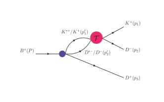
Figure 1: The diagram for process $B^{+}$$\to$$D^{+}D^{-}K^{+}$ with $D^{*-}K^{*+}-{D^{-}}{K^{+}}$ rescattering.

First, we need to deal with the direct vertex $B^{+}$ $\to$ $D^{+}D^{(*)-}K^{(*)+}$, as shown in the blue full circle in Fig. 1. Following Ref. Braaten:2004fk , the amplitude of the three-body decay can be constrained by Lorentz invariance. For direct decay $B^{+}$$\to$$D^{+}D^{-}K^{+}$, the amplitude has the form $A_{B^{+}\to D^{+}D^{-}K^{+}}=c_{1}$, and for direct decay $B^{+}\to D^{+}D^{*-}K^{*+}$, it takes the form $A_{B^{+}\to D^{+}D^{*-}K^{*+}}=c_{2}\epsilon_{D^{*-}}\epsilon_{K^{*+}}$, where $\epsilon_{D^{*-}}$ and $\epsilon_{K^{*+}}$ are the polarization vectors of $D^{*-}$ and $K^{*+}$, respectively. The constants $c_{1}$ and $c_{2}$ represent the coupling constants for the respective channels. The value of $c_{1}$ can be obtained by multiplying the branching fraction of the $B^{+}$$\to$$D^{+}D^{-}K^{+}$ with the decay width of the $B^{+}$ meson. The branching fraction for $B^{+}$$\to$$D^{+}D^{-}K^{+}$ is $\mathcal{B}_{B^{+}\to D^{+}D^{-}K^{+}}=(2.2\pm 0.7)\times 10^{-4}$LHCb:2022dvn . However, the branching fraction for $B^{+}$$\to$$D^{+}D^{-}K^{+}$ is not yet available. Therefore, we use $c_{1}=5.397\times 10^{-5}$, as mentioned in Ref. Ding:2023yuo , and treat $c_{2}$ as a free parameter to estimate the decay process due to the lack of experimental information. The determination of $c_{2}$ will be refined based on the experimental data for the process $B^{+}$ $\to$ $D^{+}D^{(*)-}K^{(*)+}$.

The next step is to construct the potential kernel ${\cal T}$ for the rescattering process, as shown in Fig. 1, to find the pole in the complex energy plane within the qBSE approach and to calculate the invariant mass spectrum. The one-boson exchange model will be adopted, with light mesons $\pi$, $\eta$, $\eta^{\prime}$, $\rho$, and $\omega$ mediating the interaction between $D^{(*)-}$ and $K^{(*)+}$ mesons. For the systems considered in this work, the couplings of exchanged light mesons to charmed mesons and strange mesons are required. Thus, the hidden-gauge Lagrangians with SU(4) symmetry are suitable for constructing the potential, which reads Bando:1984ej ; Bando:1987br ; Nagahiro:2008cv

$$\mathcal{L}_{\mathcal{PP}\mathcal{V}} =-ig~{}\langle V_{\mu}[\mathcal{P},\partial^{\mu}\mathcal{P}]\rangle,$$

$$\mathcal{L}_{\mathcal{VV}\mathcal{P}} =\frac{G^{\prime}}{\sqrt{2}}~{}\epsilon^{\mu\nu\alpha\beta}\langle\partial_{\mu}\mathcal{V}_{\nu}\partial_{\alpha}\mathcal{V}_{\beta}\mathcal{P}\rangle,$$

$$\mathcal{L}_{\mathcal{VV}\mathcal{V}} =ig~{}\langle(\mathcal{V}_{\mu}\partial^{\nu}\mathcal{V}^{\mu}-\partial^{\nu}\mathcal{V}_{\mu}\mathcal{V}^{\mu})\mathcal{V}_{\nu}\rangle,$$ (1)

with $G^{\prime}={3g^{\prime 2}}/{4\pi^{2}f_{\pi}}$, $g^{\prime}=-{G_{\mathcal{V}}m_{\rho}}/{\sqrt{2}{f_{\pi}}^{2}}$, $G_{\mathcal{V}}\simeq 55$ MeV and $f_{\pi}=93$ MeV and the coupling constant $g=M_{\mathcal{V}}/{2f_{\pi}}$, $M_{\mathcal{V}}\simeq 800$ MeV Nagahiro:2008cv . The $\mathcal{P}$ and $\mathcal{V}$ are the pseudoscalar and vector matrices under SU(4) symmetry as

$${{\mathcal{P}}}=\left(\begin{array}[]{cccc}\frac{\sqrt{3}\pi^{0}+\sqrt{2}\eta+\eta^{\prime}}{\sqrt{6}}&\pi^{+}&K^{+}&\bar{D}^{0}\\ \pi^{-}&\frac{-\sqrt{3}\pi^{0}+\sqrt{2}\eta+\eta^{\prime}}{\sqrt{6}}&K^{0}&D^{-}\\ K^{-}&\bar{K}^{0}&\frac{-\eta+\sqrt{2}\eta^{\prime}}{\sqrt{3}}&D_{s}^{-}\\ D^{0}&D^{+}&D_{s}^{+}&\eta_{c}\\ \end{array}\right),\,$$ (2)

and

$${\mathcal{V}}=\left(\begin{array}[]{cccc}\frac{\rho^{0}+\omega}{\sqrt{2}}&\rho^{+}&K^{*+}&\bar{D}^{*0}\\ \rho^{-}&\frac{-\rho^{0}+\omega}{\sqrt{2}}&K^{*0}&{D}^{*-}\\ K^{*-}&\bar{K}^{*0}&\phi&D_{s}^{*-}\\ D^{*0}&D^{*+}&D_{s}^{*+}&J/\psi\\ \end{array}\right)\,.$$ (3)

2.2 Mechanism for $D_{s}^{+}D_{s}^{-}-{D^{+}}{D^{-}}$ rescattering

In this work, we explore the $\chi_{c0}(3930)$ resonance structure in the ${D^{+}}{D^{-}}$ invariant mass spectrum, which can be related to $D_{s}^{+}D_{s}^{-}-{D^{+}}{D^{-}}$ rescattering Ding:2023yuo . The Feynman diagram of such processes is illustrated in Fig. 2. The $B^{+}$ meson decays to $D_{(s)}^{+}D_{(s)}^{-}$ and $K^{+}$ first, and the intermediate $D_{(s)}^{+}D_{(s)}^{-}$ channel will be involved in the rescattering process, subsequently obtaining the final product $D^{+}D^{-}$. The amplitude of direct $B^{+}$$\to$$D_{(s)}^{+}D_{(s)}^{-}K^{+}$, as shown as the blue full circle in Fig. 2, can be written as ${\cal M}_{B^{+}\to D_{(s)}^{+}D_{(s)}^{-}K^{+}}=c_{3}(c_{1})$, where $c_{3}=6.027\times 10^{-5}$ and $c_{1}=5.397\times 10^{-5}$ as mentioned in Ref. Ding:2023yuo and Sec. 2.1.

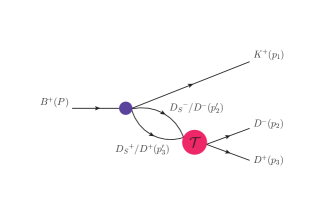
Figure 2: The diagram for process $B^{+}\to D^{+}D^{-}K^{+}$ with $D_{s}^{+}D_{s}^{-}-{D^{+}}{D^{-}}$ rescattering in.

For the S-wave isoscalar $D_{s}^{+}D_{s}^{-}$ and ${D^{+}}{D^{-}}$ states, the wave functions can be constructed as

$$|X_{D\bar{D}}^{0}\rangle =\frac{1}{\sqrt{2}}\left(|D^{+}\bar{D}^{-}\rangle+|D^{0}\bar{D}^{0}\rangle\right),\ |X_{D_{s}\bar{D}_{s}}^{0}\rangle=|D_{s}^{-}D_{s}^{+}\rangle,$$ (4)

The one-boson-exchange model is used to obtain the interaction between the heavy mesons. Contributions from vector mesons ($\mathbb{V}=\rho$ and $\omega$ for ${D^{+}}{D^{-}}-{D^{+}}{D^{-}}$ interaction, $\mathbb{V}=\phi$ for ${D_{s}}^{+}{D_{s}}^{-}-{D_{s}}^{+}{D_{s}}^{-}$ interaction, and $\mathbb{V}=K^{*}$ for ${D^{+}}{D^{-}}-{D_{s}}^{+}{D_{s}}^{-}$ interaction) and scalar meson ($\sigma$) exchange are considered. Different from the $D^{(*)-}K^{(*)+}$ channel, two charmed mesons are involved here. Hence, heavy quark symmetry is more suitable to describe the interaction. The heavy quark effective Lagrangian for heavy mesons interacting with light mesons reads Cheng:1992xi ; Yan:1992gz ; Wise:1992hn ; Burdman:1992gh ; Casalbuoni:1996pg ,

$$\mathcal{L}_{\mathcal{PP}\mathbb{V}} =-\sqrt{2}\beta{}g_{V}\mathcal{P}_{b}\mathcal{P}_{a}^{{\dagger}}v\cdot{\mathbb{V}}_{ba}+\sqrt{2}\beta{}g_{V}\widetilde{\mathcal{P}}^{{\dagger}}_{a}\widetilde{\mathcal{P}}_{b}v\cdot{\mathbb{V}}_{ab},$$

$$\mathcal{L}_{\mathcal{PP}\sigma} =-2g_{s}\mathcal{P}_{b}\mathcal{P}^{{\dagger}}_{b}\sigma-2g_{s}\widetilde{\mathcal{P}}_{b}\widetilde{\mathcal{P}}^{{\dagger}}_{b}\sigma,$$ (5)

where the velocity $v$ should be replaced by $i\overleftrightarrow{\partial}/2\sqrt{m_{i}m_{f}}$ with $m_{i,f}$ being the mass of the initial or final heavy meson. ${\mathcal{P}}^{(*)T}=(D^{(*)0},D^{(*)+},D_{s}^{(*)+})$. The $\mathbb{V}$ denotes the SU(3) vector matrix, whose elements are the first $3\times 3$ elements of the SU(4) vector matrix in Eq. (3). The parameters involved here were determined in the literature as $\beta=0.9$, $g_{s}=0.76$, and $g_{V}=5.9$ Falk:1992cx ; Isola:2003fh ; Liu:2009qhy ; Chen:2019asm .

Besides, contribution from the $J/\psi$ exchange is also considered in the current work since it is found important in the interaction between charmed and anticharmed mesons Ding:2023yuo . The Lagrangians are written with the help of heavy quark effective theory as Casalbuoni:1996pg ; Oh:2000qr ,

$${\cal L}_{D_{(s)}\bar{D}_{(s)}J/\psi} =ig_{D_{(s)}D_{(s)}\psi}\psi\cdot\bar{D}\overleftrightarrow{\partial}D,$$ (6)

where the couplings are related to a single parameter $g_{2}$ as ${g_{D_{(s)}D_{(s)}\psi}}/{m_{D}}=2g_{2}\sqrt{m_{\psi}}$,with $g_{2}={\sqrt{m_{\psi}}}/({2m_{D}f_{\psi}})$ and $f_{\psi}=405$ MeV.

2.3 Potential kernel

With the above Lagrangians, the potential kernel in the one-boson-exchange model can be constructed using the standard Feynman rules, expressed as

$${\cal V}_{P,\sigma}=I_{{i}}\Gamma_{1}\Gamma_{2}P_{{P},\sigma}f_{P,\sigma}^{2}(q^{2}),$$

$${\cal V}_{V}=I_{{i}}\Gamma_{1\mu}\Gamma_{2\nu}P^{\mu\nu}_{V}f_{V}^{2}(q^{2}),$$ (7)

for pseudoscalar ($P$), scalar ($\sigma$), and vector ($V$) exchange, respectively. The $\Gamma_{1}$ and $\Gamma_{2}$ are for the upper and lower vertices of the one-boson-exchange Feynman diagram, respectively. The $I_{i}$ is the flavor factor for certain meson exchange which can be derived using the Lagrangians in Eqs (2.1), (5) and (6) and the matrices in Eqs. (2) and (3) He:2015mja . The explicit values are $I_{\pi}=-3/2$, $I_{\eta}=0$, $I_{\eta^{\prime}}=1/2$, $I_{\rho}=-3/2$ and $I_{\omega}=1/2$ for $D^{*-}K^{*+}$$-$${D^{-}}{K^{+}}$ rescattering, and $I_{\rho}=3/2$, $I_{\omega}=1/2$, $I_{\sigma}=I_{J/\psi}=I_{\phi}=1$ for $D_{s}^{+}D_{s}^{-}-{D^{+}}{D^{-}}$ rescattering, respectively. The propagators are defined as usual as

$$P_{{P,\sigma}}=\frac{i}{q^{2}-m_{{P},{\sigma}}^{2}},\ \ P^{\mu\nu}_{V}=i\frac{-g^{\mu\nu}+q^{\mu}q^{\nu}/m^{2}_{V}}{q^{2}-m_{V}^{2}},$$ (8)

where $q$ is the momentum of exchanged meson and $m_{V,P,\sigma}$ represents the mass of the exchanged meson. We introduce a form factor $f(q^{2})=\Lambda_{e}^{2}/(q^{2}-\Lambda_{e}^{2})$ with a cutoff $\Lambda_{e}$ to compensate for the off-shell effect of the exchanged meson. This form factor type was also adopted in Ref. Gross:2008ps for studying nucleon-nucleon scattering with spectator approximation, similar to the current work. It helps in avoiding overestimation of the contribution of $J/\psi$ exchange in $D_{s}^{+}D_{s}^{-}-{D^{+}}{D^{-}}$ rescattering in the current work.

2.4 Rescattering amplitudes in qBSE approach

The amplitude of the rescattering process will be expressed within the qBSE approach. Note that the diagrams illustrated in Sec.2.1 and Sec.2.2 involve the same initial and final particles but different intermediate particles. Here, we present only the rescattering amplitude of the system mentioned in Sec.2.1, where the final particles $K^{+}$, $D^{-}$, and $D^{+}$ are labeled as particles 1, 2, and 3, respectively. The rescattering amplitude for the system discussed in Sec.2.2 can be obtained analogously.

Based on the potential of the interactions constructed above, the rescattering amplitude can be obtained using the qBSE approach He:2014nya ; He:2015mja ; He:2017lhy ; He:2015yva ; He:2017aps . After the partial-wave decomposition, the qBSE can be reduced to a 1-dimensional equation for scattering amplitude ${{\cal T}}^{J^{P}}$ with a spin-parity $J^{P}$ as He:2015mja ,

$$i{{\cal T}}^{J^{P}}_{\lambda^{\prime}_{1},\lambda^{\prime}_{2},\lambda_{1},\lambda_{2}}({\rm p}^{\prime},{\rm p})$$

$$=i{{\cal V}}^{J^{P}}_{\lambda^{\prime}_{1},\lambda^{\prime}_{2},\lambda_{1},\lambda_{2}}({\rm p}^{\prime},{\rm p})+\frac{1}{2}\sum_{\lambda^{\prime\prime}_{1},\lambda^{\prime\prime}_{2}}\int\frac{{\rm p}^{\prime\prime 2}d{\rm p}^{\prime\prime}}{(2\pi)^{3}}$$

$$\cdot i{{\cal V}}^{J^{P}}_{\lambda^{\prime}_{1},\lambda^{\prime}_{2},\lambda^{\prime\prime}_{1},\lambda^{\prime\prime}_{2}}({\rm p}^{\prime},{\rm p}^{\prime\prime})G_{0}({\rm p}^{\prime\prime})i{{\cal T}}^{J^{P}}_{\lambda^{\prime\prime}_{1},\lambda^{\prime\prime}_{2},\lambda_{1},\lambda_{2}}({\rm p}^{\prime\prime},{\rm p}),\quad\quad$$ (9)

where the indices $\lambda^{\prime}_{1}$, $\lambda^{\prime}_{2}$, $\lambda^{\prime\prime}_{1}$, $\lambda^{\prime\prime}_{2}$, $\lambda_{1}$, $\lambda_{2}$ represent the helicities of the two rescattering constituents for the final, intermediate, and initial particles 1 and 2, respectively. $G_{0}({\bm{p}}^{\prime\prime})$ is a reduced propagator written in the center-of-mass frame, with $P=(M,{\bm{0}})$ as

$$G_{0} =\frac{\delta^{+}(p^{\prime\prime~{}2}_{2}-m_{2}^{2})}{p^{\prime\prime~{}2}_{1}-m_{1}^{2}}$$

$$=\frac{\delta^{+}(p^{\prime\prime 0}_{2}-E_{2}({\bm{p}}^{\prime\prime}))}{2E_{2}({\bm{p}^{\prime\prime}})[(W-E_{2}({\bm{p}}^{\prime\prime}))^{2}-E_{1}^{2}({\bm{p}}^{\prime\prime})]},$$ (10)

where $m_{1,2}$ is the mass of particle 1 or 2. As required by the spectator approximation, the heavier particle (particle 2 here) is put on shell, with a four-momentum of $p^{\prime\prime 0}_{2}$$=$$E_{2}({\rm p}^{\prime\prime})$$=$$\sqrt{m_{2}^{~{}2}+\rm p^{\prime\prime 2}}$. The corresponding four-momentum for the lighter particle (particle 1 here) $p^{\prime\prime 0}_{1}$ is then $W-E_{2}({\rm p}^{\prime\prime})$ with $W$ being the center-of-mass energy of the system. Here and hereafter we define the value of the momentum ${\rm p}=|{\bm{p}}|$. And the momentum of particle 1 ${\bm{p}}^{\prime\prime}_{1}=-{\bm{p}}^{\prime\prime}$ and the momentum of particle 2 ${\bm{p}}^{\prime\prime}_{2}={\bm{p}}^{\prime\prime}$.

The partial wave potential ${\cal V}_{\lambda^{\prime}_{1},\lambda^{\prime}_{2},\lambda_{1},\lambda_{2}}^{J^{P}}$ can be obtained from the potential as

$$i{\cal V}_{\lambda^{\prime}_{1},\lambda^{\prime}_{2},\lambda_{1},\lambda_{2}}^{J^{P}}({\rm p}^{\prime},{\rm p}) =2\pi\int d\cos\theta~{}[d^{J}_{\lambda_{21}\lambda^{\prime}_{21}}(\theta)i{\cal V}_{\lambda^{\prime}_{1}\lambda^{\prime}_{2},\lambda_{1}\lambda_{2}}({\bm{p}}^{\prime},{\bm{p}})$$

$$+\eta d^{J}_{-\lambda_{21}\lambda^{\prime}_{21}}(\theta)i{\cal V}_{\lambda^{\prime}_{1},\lambda^{\prime}_{2},-\lambda_{1},-\lambda_{2}}({\bm{p}}^{\prime},{\bm{p}})],$$ (11)

where $\eta=PP_{1}P_{2}(-1)^{J-J_{1}-J_{2}}$ with $P$ and $J$ being parity and spin for system and constituent 1 or 2. $\lambda_{21}=\lambda_{2}-\lambda_{1}$. The initial and final relative momenta are chosen as ${\bm{p}}^{\prime}=(0,0,{\rm p}^{\prime})$ and ${\bm{p}}=({\rm p}\sin\theta,0,{\rm p}\cos\theta)$. The $d^{J}_{\lambda^{\prime}\lambda}(\theta)$ is the Wigner d-matrix. An exponential regularization is also introduced as a form factor into the reduced propagator as $G_{0}({\rm p}^{\prime\prime})\to G_{0}({\rm p}^{\prime\prime})e^{-2(p^{\prime\prime 2}_{2}-m_{2}^{2})^{2}/\Lambda_{r}^{4}}$ He:2015mja . The cutoff parameter $\Lambda_{r}$ and $\Lambda_{e}$ can be chosen as different values, but have a similar effect on the result. For simplification, we set $\Lambda_{r}=\Lambda_{e}$ in the current work.

The amplitude ${\cal T}$ can be determined by discretizing the momenta ${\rm p}^{\prime}$, ${\rm p}$, and ${\rm p}^{\prime\prime}$ in the integral equation (9) using Gauss quadrature with a weight $w({\rm p}_{i})$. After this discretization, the integral equation can be reformulated as a matrix equation  He:2015mja

$${T}_{ik} ={V}_{ik}+\sum_{j=0}^{N}{V}_{ij}G_{j}{T}_{jk}.$$ (12)

Here, the propagator $G$ is represented as a diagonal matrix:

$$G_{j>0} =\frac{w({\rm p}^{\prime\prime}_{j}){\rm p}^{\prime\prime 2}_{j}}{(2\pi)^{3}}G_{0}({\rm p}^{\prime\prime}_{j}),$$

$$G_{j=0} =-\frac{i{\rm p}^{\prime\prime}_{o}}{32\pi^{2}W}+\sum_{j}\left[\frac{w({\rm p}_{j})}{(2\pi)^{3}}\frac{{\rm p}^{\prime\prime 2}_{o}}{2W{({\rm p}^{\prime\prime 2}_{j}-{\rm p}^{\prime\prime 2}_{o})}}\right],$$ (13)

where the on-shell momentum is given by

$${\rm p}^{\prime\prime}_{o}=\frac{1}{2W}\sqrt{[W^{2}-(m_{1}+m_{2})^{2}][W^{2}-(m_{1}-m_{2})^{2}]}.$$ (14)

To identify the pole of the rescattering amplitude in the energy complex plane, we seek the position where $|1-{V}G|=0$ with $z=E_{R}+i\Gamma/2$ corresponding to the total energy and width.

After incorporating the amplitudes of the direct decay and rescattering processes, the total amplitude of the process $B^{+}$$\to$$D^{+}D^{-}K^{+}$ with $D^{*-}K^{*+}$$-$${D^{-}}{K^{+}}$ rascattering can be expressed in the center-of-mass frame of particles 1 and 2 as follows He:2017lhy ; Ding:2023yuo :

$${\cal M}(p_{1},p_{2},p_{3}) =\sum_{\lambda^{\prime}_{1},\lambda^{\prime}_{2}}\int\frac{d^{4}p^{\prime cm}_{2}}{(2\pi)^{4}}{\cal T}_{\lambda^{\prime}_{1},\lambda^{\prime}_{2}}(p^{cm}_{1},p^{cm}_{2};p^{\prime cm}_{1},p^{\prime cm}_{2})$$

$$\cdot\ G_{0}(p^{\prime cm}_{2}){\cal A}_{\lambda^{\prime}_{1},\lambda^{\prime}_{2}}(p^{\prime cm}_{1},p^{\prime cm}_{2},p_{3}^{cm}).$$ (15)

Here, the helicities of the initial and final particles of the process $B^{+}\to D^{+}D^{-}K^{+}$ have been omitted since they are all zero. The momenta with the superscript $cm$ refer to those in the center-of-mass frame of particles 1 and 2.

To analyze the direct decay amplitude ${\cal A}_{\lambda^{\prime}_{1},\lambda^{\prime}_{2}}$ a partial wave expansion is required, similar to the expansion performed on the rescattering potential kernel ${\cal V}$ conducted in Eq. (11), as shown in Ref. Gross:2008ps ,

$${\cal A}_{\lambda^{\prime}_{1},\lambda^{\prime}_{2}}(p^{\prime cm}_{1},p^{\prime cm}_{2},p_{3}^{cm})=\sum_{J\lambda^{\prime}_{1}\lambda^{\prime}_{2}}N_{J}D^{J*}_{\lambda^{\prime}_{1},\lambda^{\prime}_{2}}(\Omega^{cm}_{2}){\cal A}^{J}_{\lambda^{\prime}_{1},{\lambda}^{{}^{\prime}}_{2}}({\rm p}^{\prime cm}_{2},p_{3}^{cm}),$$ (16)

where $N_{J}$ is a normalization constant with the value of $\sqrt{(2J+1)/4\pi}$, and $\Omega_{2}^{cm}$ is the spherical angle of momentum of particle 2. Hence, the partial-wave amplitude for $J^{P}=0^{+}$ is given by

$${\cal M}^{0^{+}}(p_{1},p_{2},p_{3}) =\frac{1}{2}N_{0}\sum_{\lambda^{\prime}_{1}\lambda^{\prime}_{2}}\int\frac{{\rm p}^{\prime cm2}_{2}d{\rm p}^{\prime cm}_{2}}{(2\pi)^{3}}i{\cal T}^{0^{+}}_{\lambda^{\prime}_{1},\lambda^{\prime}_{2}}({\rm p}^{\prime cm}_{2},{\rm p}^{cm}_{2})$$

$$\ \ \cdot\ \ G_{0}({\rm p}^{\prime cm}_{2}){\cal A}^{0^{+}}_{\lambda^{\prime}_{1},\lambda^{\prime}_{2}}({\rm p}^{\prime cm}_{2},p_{3}^{cm}).$$ (17)

3 The numerical results

In this section, we will calculate the $D^{-}K^{+}$ and $D^{-}D^{+}$ invariant mass spectra and generate the corresponding Dalitz plot using Monte Carlo simulation. Our analysis aims to compare these results with experimental data to investigate the nature of the $X_{0}(2900)$ and $\chi_{c0}(3930)$ states.

3.1 Invariant mass spectrum and Dalitz plot

With the reparation in the previous section, we are able to calculate the decay amplitude of the process $B^{+}$$\to$$D^{+}D^{-}K^{+}$ with rescattering of $D^{*-}K^{*+}$$-$$D^{-}K^{+}$ with $J^{P}=0^{+}$ for the $X_{0}(2900)$ resonance. Similarly, we can obtain the decay amplitude for $D_{s}^{+}D_{s}^{-}-{D}^{+}{D}^{-}$ with $J^{P}=0^{+}$ for $\chi_{c0}(3930)$ resonance using a similar approach.

In the current works, we focus on the roles played by rescatterings and relevant molecular states process $B^{+}\to D^{+}D^{-}K^{+}$. However, it is important to note that if we only consider rescatterings related to the $X_{0}(2900)$ and $\chi_{c0}(3930)$ resonances, the model amplitude may be too simplistic to accurately replicate the invariant mass spectra observed in experiments. To address this, we introduce Breit-Wigner resonances near 2900 MeV with $J=1$, near 3770 MeV with $J=1$, and near 3930 MeV with $J=2$ to account for the $X_{1}(2900)$, $\psi(3770)$ and $\chi_{c2}(3930)$ signals observed by the LHCb Collaboration. The amplitude model can be expressed as,

$$A(J)=a_{J}BW(M_{ab})\times T(\Omega).$$ (18)

Here $a_{J}$ is a free parameter. The relativistic Breit-Wigner function $BW(M_{ab})$ is defined as,

$$BW\left(M_{ab}\right)=\frac{F_{r}F_{D}}{M_{r}^{2}-M_{ab}^{2}-i\Gamma_{ab}M_{r}},$$ (19)

where $F_{r}$ and $F_{D}$ represent the Blatt-Weisskopf damping factors for the $B$ meson and the resonance, respectively. $M_{r}$ is the mass of resonance, $M_{ab}$ is the invariant mass while $ab$ denotes $12$ or $23$ depending on the system we choose, and $\Gamma_{ab}$ is the mass-dependent width, which can be expressed as

$$\Gamma_{ab} =\Gamma_{r}\left(\frac{p_{ab}}{p_{r}}\right)^{2J+1}\left(\frac{M_{r}}{M_{ab}}\right)F_{r}^{2}.$$

$$p_{ab} =\frac{\sqrt{\left(M_{ab}^{2}-m_{a}^{2}-m_{b}^{2}\right)^{2}-4m_{a}^{2}m_{b}^{2}}}{2M_{ab}},$$ (20)

where $\Gamma_{r}$ and $J$ are the width and the spin of the resonance. The quantity $p_{ab}$ is the momentum of either daughter in the $ab$ rest frame, and $p_{r}$ is the value of $p_{ab}$ when $M_{ab}=M_{r}$. The exact expressions of the Blatt-Weisskopf factors Blatt:1952ije are given in Ref. BaBar:2010wqe . The angular term $T(\Omega)$ is also given in Ref. BaBar:2010wqe and depends on the masses of the particles involved in the reaction as well as on the spin of the intermediate resonance.

The parameters associated with the additional $X_{1}(2900)$, $\psi(3770)$ and $\chi_{c2}(3930)$ resonances are predetermined based on the experimental values LHCb:2020bls ; LHCb:2020pxc . The predetermined masses and widths are provided in Table 2. Additionally, the resonances resulting from the rescatterings correspond to poles in the complex energy plane. By adjusting the masses and widths to better match the invariant mass spectra, the values for the masses and widths of $X_{0}(2900)$ and $\chi_{c0}(3930)$ are also determined and included in Table 2. Further discussion on these values will be provided later.

Table 2: Masses and widths for the resonances involved. Predetermined values are cited from Refs. LHCb:2020bls ; LHCb:2020pxc , and the fitted values are determined by fitting the invariant mass spectra.

	Resonance	Mass (MeV)	Width (MeV)
Predetermiend	$X_{1}(2900)$	2904.0	110.0
	$\psi(3770)$	3778.1	0.9
	$\chi_{c2}(3930)$	3926.8	34.2
Fitted	$X_{0}(2900)$	2884.9	62.0
	$\chi_{c0}(3930)$	3923.9	0.1

Besides, a parameterized background contribution is introduced into the $D^{-}K^{+}$ invariant mass distribution from rescattering described in Sec. 3.2, which can be written as

$$\hat{\cal A}^{bk}(M_{12})=e^{d(i\pi)}c(M_{12}-M_{min})^{a}(M_{max}-M_{12})^{b},$$ (21)

where the parameters for the background are chosen as $(a,b,c,d)=(4.0,0.5,5.6,0.5)$ to fit the experimental data.

The total decay width incorporating all these contributions to the amplitude ${\cal M}(p_{1},p_{2},p_{3})$ can be expressed as

$${d\Gamma} =\frac{(2\pi)^{4}}{2M_{B}}|{\cal M}(p_{1},p_{2},p_{3})|^{2}d\Phi_{3},$$ (22)

where $M_{B}$ are the mass of initial $B^{+}$ meson. In this work, the phase space $d\Phi_{3}$ in Eq. (22) is obtained using the GENEV code in FAWL, which employs the Monte Carlo method to generate events of the three-body final state. The phase space is defined as,

$$R_{3}=(2\pi)^{5}d\Phi_{3}=\prod_{i}^{3}\frac{d^{3}p_{i}}{2E_{i}}\delta^{4}\left(\sum_{i}^{n}p_{i}-P\right),$$ (23)

where $p_{i}$ and $E_{i}$ provided by the code represent the momentum and energy of the final particle $i$. By simulating $5\times 10^{5}$ events, the event distribution can be obtained, allowing for the visualization of the Dalitz plot and the invariant mass spectra with respect to $m_{D^{-}K^{+}}$ and $m_{D^{+}D^{-}}$.

It is important to note that an overall scaling factor for the invariant mass spectra cannot be determined due to the absence of information on the total number of $B^{+}$ candidates, which was not provided by the LHCb collaboration. Therefore, it is necessary to scale the theoretical decay distribution to the experimental data to facilitate a comparison between theoretical predictions and experimental results. It is crucial to emphasize that this scaling factor renders only the relative values of the coupling constants $c_{1}$, $c_{2}$ and $c_{3}$ meaningful. Additionally, the cutoff parameter $\Lambda_{e}$ is fine-tuned to best match the experimental data. Given that the interaction mechanisms differ between the $D^{*-}K^{*+}-{D^{-}}{K^{+}}$ rescattering and ${D_{s}}^{+}{D_{s}}^{-}-{D^{+}}{D^{-}}$ rescattering, the cutoff values $\Lambda_{e}$ for two rescatterings are adjusted to 3.3 and 1.8 GeV, respectively, to ensure a good fit to the experimental data.

3.2 $D^{-}K^{+}$ invariant mass spectrum and $X_{0,1}(2900)$

As shown in Fig. 3, the LHCb data suggest an obvious resonance structure around 2900 MeV in the $D^{-}K^{+}$ invariant mass spectrum of the process $B^{+}$$\to$$D^{+}D^{-}K^{+}$. Such a structure is close to the $D^{*}K^{*}$ threshold and was explained as $D^{*-}K^{*+}$ molecular states in the literature. As we can see from the blue dashed curve representing the contribution from $D^{*-}K^{*+}$$-$${D^{-}}{K^{+}}$ rescattering in Fig. 3, an obvious peak is produced near 2885 MeV as expected, which can be related to the $X_{0}(2900)$ resonance. However, a satisfactory fit of the LHCb’s data cannot be obtained if the $X_{1}(2900)$ is not included, as shown by the gray line in Fig. 3, because it seems narrow and located to the left compared to the experimental structure. In the experimental article LHCb:2020pxc , the structure observed near 2900 MeV is suggested to be formed by two states, $X_{0}(2900)$ and $X_{1}(2900)$, with $X_{0}(2900)$ having a smaller mass and width. Thus, we introduce a Breit-Wigner resonance near 2900 MeV with $J=1$ to fit the $X_{1}(2900)$ structure, which can be written as Eq. (18)-(20) with predetermined mass and width listed in Table 2.

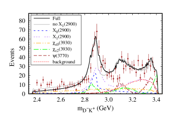
Figure 3: The $D^{-}K^{+}$ invariant mass spectrum for $B^{+}\to D^{+}D^{-}K^{+}$ decay. The black (grey) full curve shows the contribution from the total amplitude (without $X_{1}(2900)$), and the blue, orange, green, brown, purple, and red dashed curves show the contributions from $X_{0}(2900)$, $\chi_{c0}(3930)$, $\chi_{c2}(3930)$, $\psi(3770)$, $X_{1}(2900)$, and background, respectively. The red points with error bars are the data from the LHCb experiment cited from Ref. LHCb:2020pxc .

A good description of the region near 2900 MeV is obtained after including the $X_{1}(2900)$ contribution, together with reflections from the $D^{+}D^{-}$ structures. The peak near 2900 MeV becomes wider and is in better agreement with the experimental result, as shown by the black curve. Thus, our result still supports the assumption of $X_{0}(2900)$ as an S-wave $D^{-}K^{+}$ molecular state, and the $X_{1}(2900)$ state is necessary to describe the structure near 2900MeV as well.

Two bumps can be observed around 3.0 to 3.5 GeV due to the contribution of $\psi(3770)$ and $\chi_{c2}(3930)$ states, which is consistent with the relevant data analysis of the LHCb Collaboration LHCb:2020pxc . No clear peak structure but a background-like signal can be found from the orange dashed curve representing the $\chi_{c0}(3930)$ state, indicating that this state has no significant contribution to the $D^{-}K^{+}$ invariant mass spectrum in our model.

3.3 ${D}^{+}{D}^{-}$ invariant mass spectrum and $\chi_{c0}(3930)$

In the ${D}^{+}{D}^{-}$ invariant mass spectra of the process $B^{+}\to D^{+}D^{-}K^{+}$, two prominent resonance structures are observed around 3770 and 3930 MeV, respectively. In our previous study, we investigated the $D_{s}^{+}D_{s}^{-}$$-$$D^{+}D^{-}$ rescattering within the ${D}^{+}{D}^{-}$ invariant mass spectrum to explore the origins of $X(3960)$ and $\chi_{c0}(3930)$. Our findings indicated that the peak attributed to $\chi_{c0}(3930)$ was too narrow to fully explain the experimental structure around 3930 MeV Ding:2023yuo . Given that this structure is suggested to arise from two states, $\chi_{c0}(3930)$ and $\chi_{c2}(3930)$, it is reasonable to propose that $\chi_{c2}(3930)$ plays a crucial role in forming the resonance near 3930 MeV in the ${D}^{+}{D}^{-}$ invariant mass spectrum. Additionally, a distinct structure around 3770 MeV is identified as $\psi(3770)$ with spin parity $J^{PC}=1^{--}$ in experimental reports. Therefore, in this study, Breit-Wigner resonances with $J=2$ near 3930 MeV and $J=1$ near 3770 MeV are introduced to model the $\chi_{c2}(3930)$ and $\psi(3770)$ structures, respectively. These resonances are parameterized according to Eq. (18)-(20) with predetermined mass and width listed in Table 2.

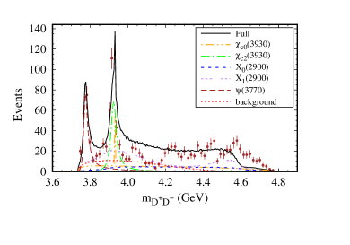
Figure 4: The $D^{+}D^{-}$ invariant mass spectrum for $B^{+}\to D^{+}D^{-}K^{+}$ decay. The black solid curve shows the contribution from the total amplitude, and the orange, green, brown, blue, purple, and red dashed curves show the contributions from $\chi_{c0}(3930)$, $\chi_{c2}(3930)$, $\psi(3770)$, $X_{0}(2900)$, $X_{1}(2900)$, and the background, respectively. The red points with error bars are the data from the LHCb experiment cited from Ref. LHCb:2020pxc .

The $D^{+}D^{-}$ invariant mass spectrum for $B^{+}\to D^{+}D^{-}K^{+}$ via the intermediate states $\chi_{c0}(3930)$, $\chi_{c2}(3930)$, $\psi(3770)$, $X_{0}(2900)$, and $X_{1}(2900)$ can be obtained in Fig. 4. As shown in the orange dashed curve representing the contribution of $\chi_{c0}(3930)$ state in Fig. 4, a significant but extremely narrow peak around 3930 MeV can be observed, which can be associated with the rescattering of $D_{s}^{+}D_{s}^{-}$$-$${D}^{+}{D}^{-}$ channels. After overlapping the Breit-Wigner resonance introduced to fit the $\chi_{c2}(3930)$ structure, the width of the peak around 3930 MeV becomes larger as the black curve shows, and the explicit shape of the experimental structure can be better fitted compared with our previous work. This result favors the assumption of the $\chi_{c0}(3930)$ as an S-wave $D^{+}D^{-}$ molecular state but may play a minor role in forming the structure around 3930 MeV in the $D^{+}D^{-}$ invariant mass spectrum. Meanwhile, one can also find a peak near 3770 MeV, which is due to the Breit-Wigner resonance we introduced to fit the $\psi(3770)$ structure. We do not focus our attention on the structure in the higher energy region because the real mechanism (which is suggested to include the contribution of the $\psi(4040)$, $\psi(4160)$, and $\psi(4415)$ together with reflections from the $D^{-}K^{+}$ structures by LHCb LHCb:2020pxc ) is much more complex than our model. No significant peak structure can be found in the blue dashed curve in Fig. 4, which indicates that $X_{0}(2900)$ has no particular contribution in the $D^{+}D^{-}$ invariant mass spectrum.

3.4 Dalitz Plot

In the above, the invariant mass spectra for the process $B^{+}$$\to$$D^{+}D^{-}K^{+}$ is presented. To provide a more explicit picture for such process, we present the Dalitz plot against the invariant masses $m_{D^{-}K^{+}}$ and $m_{D^{+}D^{-}}$ of the final particles in the molecular state picture in Fig. 5.

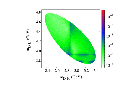
Figure 5: The Dalitz plot for the $B^{+}\to D^{+}D^{-}K^{+}$ process. The color box represents the ratio of the number of events in a bin of 0.005GeV $\times$ 0.005GeV to the total number of events. The results are obtained with $5\times 10^{5}$ simulations.

When comparing our results in Fig. 5 with the LHCb data (Figure 8 in Ref. LHCb:2020pxc ), we observe a striking similarity in the overall pattern. In the Dalitz plot, two prominent horizontal strips appear at $m_{D^{+}D^{-}}$ around 3.77 and 3.93 GeV, indicating contributions from the $\psi(3770)$ and $\chi_{c0,2}(3930)$ resonances, respectively. Additionally, a distinct vertical strip is visible at $m_{D^{-}K^{+}}$ around 2900 GeV, which can be associated with the $X_{0,1}(2900)$ states. The intermittency of these strips, observed in both our results and the experimental data from LHCb, provides additional insights. This pattern suggests that the resonances do not originate solely from scalar states, confirming the necessity of including the $\chi_{c2}(3930)$ and $X_{1}(2900)$ states.

4 Summary

In this work, we studied the $D^{-}K^{+}$ and $D^{+}D^{-}$ invariant mass spectra, as well as the Dalitz plot, for the $B^{+}$$\to$$D^{+}D^{-}K^{+}$ process, focusing on the $D^{*-}K^{*+}$$-$$D^{-}K^{+}$ and $D_{s}^{+}D_{s}^{-}$$-$$D^{+}D^{-}$ rescattering. This analysis assumes that resonances $X_{0}(2900)$ and $\chi_{c0}(3930)$ are $D^{*-}K^{*+}$ and $D_{s}^{+}D_{s}^{-}$ molecular states with spin parity $0^{+}$, respectively. The theoretical results, calculated using the quasipotential Bethe-Salpeter equation approach, are compared with the experimental data from the LHCb Collaboration to understand the nature of $X_{0}(2900)$ and $\chi_{c0}(3930)$.

The $D^{-}K^{+}$ invariant mass spectrum for the decay process $B^{+}\to D^{+}D^{-}K^{+}$ is examined. The $D^{*-}K^{*+}$ interaction produces a significant peak at 2886 MeV with a width of 62 MeV, identified as the $X_{0}(2900)$ contribution suggested by LHCb. However, this peak is slightly sharper than the experimental structure. Since the structure is suggested to be formed by two states, $X_{0}(2900)$ and $X_{1}(2900)$, the latter is introduced as a Breit-Wigner resonance near 2900 MeV with $J=1$ into our model. Including this state widens the structure, bringing the calculation into good agreement with the experimental $D^{-}K^{+}$ invariant mass spectrum. To describe the distribution in the higher energy region, contributions from $\psi(3770)$ and $\chi_{c2}(3930)$ are needed.

The $D^{+}D^{-}$ invariant mass spectrum, which includes contributions from the $\psi(3770)$, $\chi_{c0}(3930)$, and $\chi_{c2}(3930)$ states as suggested by LHCb, was also investigated. The $\chi_{c0}(3930)$, originating from the $D_{s}^{+}D_{s}^{-}$ interaction, exhibits a very narrow peak and plays a smaller role in forming the experimentally observed peak near 3930 MeV compared to the $\chi_{c2}(3930)$, which is introduced as a Breit-Wigner resonance. Additionally, to simulate the $\psi(3770)$ resonance, we introduced a Breit-Wigner resonance located at 3770 MeV with $J$$=$$1$. The event distribution in the $D^{+}D^{-}$ invariant mass spectrum can be described by two sharp peaks corresponding to the $\psi(3770)$ and the overlap of $\chi_{c0}(3930)$ and $\chi_{c2}(3930)$. The distribution at higher energy regions requires contributions from more states, which is not the focus of the current work and therefore not considered.

Additionally, the Dalitz plot in the $m_{D^{-}K^{+}}-m_{D^{+}D^{-}}$ plane for the process $B^{+}\to D^{+}D^{-}K^{+}$ was presented. Obvious intermittent strips are observed at about 2.90 GeV at $m_{D^{-}K^{+}}$ and 3.77 and 3.93 GeV at $m_{D^{+}D^{-}}$ in the Dalitz plot. Our calculations support the molecular interpretations for $X_{0}(2900)$ and $\chi_{c0}(3930)$ states. However, it was found necessary to include both spin-0 and spin-1 states in the $X_{J}(2900)$ region and both spin-0 and spin-2 states in the $\chi_{cJ}(3930)$ region.

References

- (1) R. Aaij et al. [LHCb], “A model-independent study of resonant structure in decays,” Phys. Rev. Lett. 125 (2020), 242001
- (2) R. Aaij et al. [LHCb], “Amplitude analysis of the decay,” Phys. Rev. D 102 (2020), 112003
- (3) R. Aaij et al. [LHCb], “Observation of new charmonium(-like) states in decays,” arXiv:2406.03156 [hep-ex]
- (4) J. R. Zhang, “Open-charm tetraquark candidate: Note on (2900),” Phys. Rev. D 103 (2021) no.5, 054019
- (5) Z. G. Wang, “Analysis of the as the scalar tetraquark state via the QCD sum rules,” Int. J. Mod. Phys. A 35 (2020) no.30, 2050187
- (6) X. G. He, W. Wang and R. Zhu, “Open-charm tetraquark and open-bottom tetraquark ,” Eur. Phys. J. C 80 (2020) no.11, 1026
- (7) G. J. Wang, L. Meng, L. Y. Xiao, M. Oka and S. L. Zhu, “Mass spectrum and strong decays of tetraquark states,” Eur. Phys. J. C 81 (2021) no.2, 188
- (8) X. H. Liu, M. J. Yan, H. W. Ke, G. Li and J. J. Xie, “Triangle singularity as the origin of and observed in ,” Eur. Phys. J. C 80 (2020) no.12, 1178
- (9) T. J. Burns and E. S. Swanson, “Kinematical cusp and resonance interpretations of the ,” Phys. Lett. B 813 (2021), 136057
- (10) R. Molina and E. Oset, “Molecular picture for the as a state and related states,” Phys. Lett. B 811 (2020), 135870 [erratum: Phys. Lett. B 837 (2023), 137645]
- (11) H. X. Chen, W. Chen, R. R. Dong and N. Su, “(2900) and (2900): Hadronic Molecules or Compact Tetraquarks,” Chin. Phys. Lett. 37 (2020) no.10, 101201
- (12) S. S. Agaev, K. Azizi and H. Sundu, “New scalar resonance X 0(2900) as a molecule: mass and width,” J. Phys. G 48 (2021) no.8, 085012
- (13) H. Mutuk, “Monte-Carlo based QCD sum rules analysis of (2900) and (2900),” J. Phys. G 48 (2021) no.5, 055007
- (14) M. Z. Liu, J. J. Xie and L. S. Geng, “ as a molecular state,” Phys. Rev. D 102 (2020) no.9, 091502
- (15) C. J. Xiao, D. Y. Chen, Y. B. Dong and G. W. Meng, “Study of the decays of wave hadronic molecules: The scalar and its spin partners ,” Phys. Rev. D 103 (2021) no.3, 034004
- (16) J. He and D. Y. Chen, “Molecular picture for and ,” Chin. Phys. C 45 (2021) no.6, 063102
- (17) S. Y. Kong, J. T. Zhu, D. Song and J. He, “Heavy-strange meson molecules and possible candidates , , and ,” Phys. Rev. D 104 (2021) no.9, 094012
- (18) R. Aaij et al. [LHCb], “Observation of a Resonant Structure near the Ds+Ds- Threshold in the Decay,” Phys. Rev. Lett. 131 (2023) no.7, 071901
- (19) M. Bayar, A. Feijoo and E. Oset, “X(3960) seen in as the X(3930) state seen in ,” Phys. Rev. D 107 (2023) no.3, 034007
- (20) Y. Chen, H. Chen, C. Meng, H. R. Qi and H. Q. Zheng, “On the nature of X(3960),” Eur. Phys. J. C 83 (2023) no.5, 381
- (21) Z. m. Ding and J. He, “Combined analysis on nature of , , and ,” Eur. Phys. J. C 83 (2023) no.9, 806
- (22) E. Braaten, M. Kusunoki and S. Nussinov, Phys. Rev. Lett. 93 (2004), 162001
- (23) R. Aaij et al. [LHCb], “First observation of the decay,” Phys. Rev. D 108 (2023), 034012
- (24) M. Bando, T. Kugo, S. Uehara, K. Yamawaki and T. Yanagida, “Is rho Meson a Dynamical Gauge Boson of Hidden Local Symmetry?,” Phys. Rev. Lett. 54 (1985), 1215
- (25) M. Bando, T. Kugo and K. Yamawaki, “Nonlinear Realization and Hidden Local Symmetries,” Phys. Rept. 164 (1988), 217-314
- (26) H. Nagahiro, L. Roca, A. Hosaka and E. Oset, “Hidden gauge formalism for the radiative decays of axial-vector mesons,” Phys. Rev. D 79 (2009), 014015
- (27) H. Y. Cheng, C. Y. Cheung, G. L. Lin, Y. C. Lin, T. M. Yan and H. L. Yu, “Chiral Lagrangians for radiative decays of heavy hadrons,” Phys. Rev. D 47 (1993), 1030-1042
- (28) T. M. Yan, H. Y. Cheng, C. Y. Cheung, G. L. Lin, Y. C. Lin and H. L. Yu, “Heavy quark symmetry and chiral dynamics,” Phys. Rev. D 46 (1992), 1148-1164 [erratum: Phys. Rev. D 55 (1997), 5851]
- (29) M. B. Wise, “Chiral perturbation theory for hadrons containing a heavy quark,” Phys. Rev. D 45 (1992) no.7, R2188
- (30) G. Burdman and J. F. Donoghue, “Union of chiral and heavy quark symmetries,” Phys. Lett. B 280 (1992), 287-291
- (31) R. Casalbuoni, A. Deandrea, N. Di Bartolomeo, R. Gatto, F. Feruglio and G. Nardulli, “Phenomenology of heavy meson chiral Lagrangians,” Phys. Rept. 281 (1997), 145-238
- (32) A. F. Falk and M. E. Luke, “Strong decays of excited heavy mesons in chiral perturbation theory,” Phys. Lett. B 292 (1992), 119-127
- (33) C. Isola, M. Ladisa, G. Nardulli and P. Santorelli, “Charming penguins in decays,” Phys. Rev. D 68 (2003), 114001
- (34) X. Liu, Z. G. Luo, Y. R. Liu and S. L. Zhu, “X(3872) and Other Possible Heavy Molecular States,” Eur. Phys. J. C 61 (2009), 411-428
- (35) R. Chen, Z. F. Sun, X. Liu and S. L. Zhu, “Strong LHCb evidence supporting the existence of the hidden-charm molecular pentaquarks,” Phys. Rev. D 100 (2019) no.1, 011502
- (36) Y. s. Oh, T. Song and S. H. Lee, “ absorption by and mesons in meson exchange model with anomalous parity interactions,” Phys. Rev. C 63 (2001), 034901
- (37) J. He, “The as a resonance from the interaction,” Phys. Rev. D 92 (2015) no.3, 034004
- (38) F. Gross and A. Stadler, “Covariant spectator theory of np scattering: Phase shifts obtained from precision fits to data below 350-MeV,” Phys. Rev. C 78 (2008), 014005
- (39) J. He, “Study of the bound states in a Bethe-Salpeter approach,” Phys. Rev. D 90 (2014) no.7, 076008
- (40) J. He and D. Y. Chen, “ as a virtual state from interaction,” Eur. Phys. J. C 78 (2018) no.2, 94
- (41) J. He, “Internal structures of the nucleon resonances and ,” Phys. Rev. C 91 (2015) no.1, 018201
- (42) J. He, “Nucleon resonances and as strange partners of LHCb pentaquarks,” Phys. Rev. D 95 (2017) no.7, 074031
- (43) J. M. Blatt and V. F. Weisskopf, “Theoretical nuclear physics,” Springer, 1952, ISBN 978-0-471-08019-0
- (44) P. del Amo Sanchez et al. [BaBar], “Dalitz plot analysis of ,” Phys. Rev. D 83 (2011), 052001