Constraining $\lambda_{B_{s}}$ by $B_{s}\to\gamma^{*}$ and $B_{s}\to\phi$ form factors

Abstract

We calculate the form factors $F_{V}(q^{2},q^{\prime 2})$ and $F_{TV}(q^{2},q^{\prime 2})$ describing the $B_{s}\to\gamma^{*}$ transition induced by the vector and tensor weak currents in a broad range of values of $q^{2}$ and $q^{\prime 2}$ far below the quark thresholds in both $q^{2}$ and $q^{\prime 2}$ channels. These form factors are calculated via the distribution amplitudes of the $B_{s}$-meson. We then interpolate the obtained results by a formula that contains pole at $q^{\prime 2}=M_{\phi}^{2}$ and extract the residue which gives the $B_{s}\to\phi$ transition form factors $V(q^{2})$ and $T_{1}(q^{2})$. In this way we obtain theoretical predictions for these form factors without invoking quark-hadron duality and QCD sum rules. Furthermore, we calculate the relationship between $V(0)$ and $T_{1}(0)$ and the parameter $\lambda_{B_{s}}(\mu)$, the inverse moment of the $B_{s}$-meson distribution amplitude. Using the available predictions for $V(0)$ and $T_{1}(0)$ coming from approaches not referring to the $B_{s}$-meson distribution amplitudes, we obtain the estimate $\lambda_{B_{s}}(\mu\simeq m_{b})=(0.62\pm 0.10)$ GeV.

1 Introduction

The inverse momentum of the distribution amplitude (2DA) $\phi_{+}$ of $B_{(s)}$-meson, $\lambda_{B_{(s)}}$, is an interesting parameter for the phenomenology of weak $B_{(s)}$ decays as it enters a number of observables related to semileptonic and multileptonic decays of $B_{(s)}$-mesons (see e.g. korchemsky2000 ; braun2017 ; beneke2020 ; bbm2023 ; bbm2024 ; wang2023 ). In spite of its importance, this parameter is presently not known with high accuracy and theoretical predictions for this parameter vary in a rather broad range, namely $\lambda_{B}(1\mbox{ GeV})=0.3\div 0.7$ GeV kou ; braun2004 ; beneke2011 ; wang2016 ; zwicky2021 ; im2022 , whereas the ratio $\lambda_{B_{s}}/\lambda_{B}$ is known with a better accuracy, $\lambda_{B_{s}}/\lambda_{B}=1.19\pm 0.14$ khodjamirian2020 .

In this paper, we discuss a new way of constraining $\lambda_{B_{s}}$.

The first step is the calculation of the form factors $F_{V}(q^{2},q^{\prime 2})$ and $F_{TV}(q^{2},q^{\prime 2})$ mk2003 ; mnk2018 describing the $B_{s}\to\gamma^{*}$ transition (see Fig. 1) in a broad range of values of $q^{2}$ and $q^{\prime 2}$ far below quark thresholds via the 2DAs of the $B_{s}$-meson. For the relevant 2DAs we make use of the local duality (LD) model of braun2017 .

Then, we interpolate these results by an analytic formula which contains a number of poles corresponding to vector meson resonances with quantum numbers appropriate to $q^{2}$ and $q^{\prime 2}$ channels. This formula is based on a dispersion representation for $F_{V,TV}(q^{2},q^{\prime 2})$ in $q^{\prime 2}$ with one subtraction mnp2004 and the spectral density of this representation is saturated by two resonances - the known lowest resonances $\phi$ and an effective vector meson pole with an unknown mass. The numerical parameters in this analytic formula are obtained by fitting the results of our calculations in a broad range of values of $q^{2}$ and $q^{\prime 2}$ far below the quark thresholds in $q^{2}$ and $q^{\prime 2}$ channels. The analytic formula contains a pole at $q^{\prime 2}=M_{\phi}^{2}$; the residue of this pole provides the $B_{s}\to\phi$ form factor $V(q^{2})$ in the case of $F_{V}$ and $T_{1}(q^{2})$ in the case of $F_{TV}$. Noteworthy, our estimate does not employ quark-hadron duality and QCD sum rules and is therefore free of the intrinsic uncertainties of the method of QCD sum rules. Our approach thus provides an interesting complementary method to the widely used method of QCD sum rules.

For comparison, we present in Appendix A the application of the standard QCD sum rule machinery braun1994 in order to calculate $T_{1}(0)$ using the $B_{s}$-meson 2DAs offen2007 . We recall that QCD sum rules calculate the residue from the very same Green function which determines the form factor $F_{TV}(q^{2},q^{\prime 2})$. However, the QCD sum-rule extraction contains auxiliary parameters (Borel parameter and effective threshold $s_{\rm eff}$) which are not fixed by any rigorous criteria, leading to uncertainties that are difficult to control. Still we observe that using some commonly adopted ways of fixing these auxiliary parameters leads to a good agreement between the estimates for $T_{1}(0)$ obtained by a direct calculation of the correlation function and extrapolation to the pole and by a direct evaluation of the residue by a quark-hadron duality Ansatz.

The approach formulated above is based on using the representations for the form factors $F_{V,TV}(q^{2},q^{\prime 2})$ up to leading-order in the strong coupling constant $\alpha_{s}$. Making use of the known radiative corrections for the form factor $F_{V}(q^{2},0)$ beneke2011 , we give arguments that for the form factors $F_{V,TV}(q^{2},q^{\prime 2})$ the radiative corrections evaluated at the scale $\mu=m_{b}$ are at the level of less than 0.5% in the broad range of values of $q^{2}$ and $q^{\prime 2}$ used in our analysis. This property means that the leading-order expression for $F_{V,TV}(q^{2},q^{\prime 2})$ expressed via the 2DAs at the scale $\mu=m_{b}$ should give a good estimate for the physical form factors $F_{V}(q^{2},q^{\prime 2})$ and $F_{TV}(q^{2},q^{\prime 2}|\mu=m_{b})$.

We then obtain the dependence of the $B_{s}\to\phi$ form factors $V(0)$ and $T_{1}(0)$ on $\lambda_{B_{s}}(\mu=m_{b})$. Combining our results with the predictions for $V(0)$ and $T_{1}(0)$ obtained by approaches not referring to 2DAs of the $B_{s}$-meson, we extract

$$\lambda_{B_{s}}(\mu\simeq m_{b})=(0.62\pm 0.10)\mbox{ GeV}.$$ (1.1)

2 The form factors $F_{V,TV}(q^{2},q^{\prime 2})$ and the $B_{s}\to\phi$ form factors $V(q^{2})$ and $T_{1}(q^{2})$

This Section provides details of the analytic calculation of $F_{V,TV}(q^{2},q^{\prime 2})$ and the corresponding numerical results.

2.1 Analytic results for $F_{V,TV}(q^{2},q^{\prime 2})$ at leading order in $\alpha_{s}$

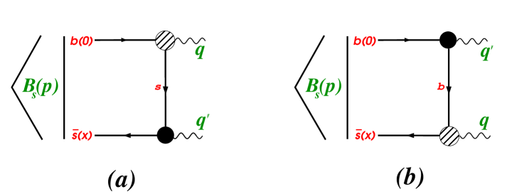
Fig. 1: (a) Diagram corresponding to the form factor $F^{(s)}_{TV}(q^{2},q^{\prime 2})$ containing $\phi$-meson pole in the $q^{\prime 2}$-channel. (b) Diagram corresponding to parametrically suppressed form factor $F^{(b)}_{TV}(q^{2},q^{\prime 2})$. The dashed blob stands for the tensor current $\bar{s}\sigma_{\mu\nu}b$ and the solid blob stands for the electromagnetic current, $j_{\alpha}^{\rm e.m.}=Q_{s}\bar{s}\gamma_{\alpha}s+Q_{b}\bar{b}\gamma_{\alpha}b$.

Let us consider the transition amplitudes involving electromagnetic and weak currents mk2003 ; mnk2018 (Fig. 1):

$$i\int dxe^{iq^{\prime}x}\langle 0|\left\{Tj_{\alpha}^{\rm e.m.}(x),\bar{s}\gamma_{\mu}q^{\nu}b(0)\right\}|\bar{B}_{s}(p)\rangle = ie\,\epsilon_{\mu\alpha qq^{\prime}}\frac{F_{V}(q^{2},q^{\prime 2})}{M_{B_{s}}},$$

$$i\int dxe^{iq^{\prime}x}\langle 0|\left\{Tj_{\alpha}^{\rm e.m.}(x),\bar{s}\sigma_{\mu\nu}q^{\nu}b(0)\right\}|\bar{B}_{s}(p)\rangle = ie\,\epsilon_{\mu\alpha qq^{\prime}}F_{TV}(q^{2},q^{\prime 2}).$$ (2.2)

The form factors $F_{i}(q^{2},q^{\prime 2})$, [$i=V,TV$] in Eq. (2.2) contains two contributions, $F_{i}=F^{(s)}_{i}+F^{(b)}_{i}$ corresponding to the diagrams in Fig. 1. We are interested in $F^{(s)}_{i}$ which contains a pole at $q^{\prime 2}=M^{2}_{\phi}$ and neglect the form factor $F^{(b)}_{i}$ parametrically suppressed by $1/m_{b}$ compared to $F^{(s)}_{i}$. So, hereafter $F_{i}$ denotes $F^{(s)}_{i}$.

The form factors $F_{i}$ may be calculated via the $B$-meson 2DAs using HQET formula (see e.g. offen2007 )

$$\langle 0|\bar{s}(x)\Gamma b(0)|\bar{B}_{s}(p)\rangle=-\frac{if_{B_{s}}M_{B_{s}}}{4}\int d\xi e^{-i\xi px}\,{\rm Tr}\bigg{\{}\gamma_{5}\Gamma(1+\not{v})\bigg{[}\phi_{+}(\xi)-\frac{\phi_{+}(\xi)-\phi_{-}(\xi)}{2vx}\not{x}\bigg{]}\bigg{\}},\quad p_{\mu}=M_{B_{s}}v_{\mu}.$$ (2.3)

Omitting all contributions at order $O(m_{s}/M_{B_{s}})$ in the numerator, one gets

$$F_{V}(q^{2},q^{\prime 2}) = -Q_{s}f_{B_{s}}M_{B_{s}}\int d\xi\bigg{[}\frac{\phi_{+}(\xi)}{m_{s}^{2}+\xi(1-\xi)M_{B_{s}}^{2}-q^{2}\xi-q^{\prime 2}(1-\xi)}+\frac{2m_{s}M_{B_{s}}\bar{\Phi}(\xi)}{(m_{s}^{2}+\xi(1-\xi)M_{B_{s}}^{2}-q^{2}\xi-q^{\prime 2}(1-\xi))^{2}}\bigg{]},$$

$$F_{TV}(q^{2},q^{\prime 2}) = -Q_{s}f_{B_{s}}M_{B_{s}}\int d\xi\frac{\phi_{+}(\xi)(1-\xi)+\bar{\Phi}(\xi)}{m_{s}^{2}+\xi(1-\xi)M_{B_{s}}^{2}-q^{2}\xi-q^{\prime 2}(1-\xi)}$$ (2.4)

with

$$\bar{\Phi}(\xi)=\int\limits_{0}^{\xi}d\xi^{\prime}\big{[}\phi_{+}(\xi^{\prime})-\phi_{-}(\xi^{\prime})\big{]}.$$ (2.5)

The kinematical singularity at $vx\to 0$ in Eq. (2.3) cannot be a singularity of the physical amplitude, so that the primitive $\bar{\Phi}(\xi)$ should vanishe at the boundaries of the 2DA support region. Then the integration by parts in $\xi$, necessary to handle the $1/vx$ term, does not contain any nonzero surface term.

For the 2DAs we use a set referred to as Model IIB in braun2017 (our $\xi$ and $\omega_{0}$ are dimensionless):

$$\phi_{+}(\xi) = \frac{5}{8\omega_{0}^{5}}\xi(2\omega_{0}-\xi)^{3}\theta(2\omega_{0}-\xi),$$ (2.6)

$$\phi_{-}(\xi) = \frac{5}{192\omega_{0}^{5}}(2\omega_{0}-\xi)^{2}\bigg{[}6(2\omega_{0}-\xi)^{2}-\frac{7(\lambda_{E}^{2}-\lambda_{H}^{2})}{M_{B_{s}}^{2}\omega_{0}^{2}}(15\xi^{2}-20\omega_{0}\xi+4\omega_{0}^{2})\bigg{]}\theta(2\omega_{0}-\xi),$$ (2.7)

where

$$\omega_{0}=\frac{5}{2}\frac{\lambda_{B_{s}}}{M_{B_{s}}}.$$ (2.8)

For numerical estimates we use $M_{B_{s}}$=5.367 GeV and $f_{B_{s}}$=0.230 GeV. The parameters $\lambda^{2}_{E,H}\simeq(0.1-0.2)$ GeV² are related to certain matrix elements of antiquark-quark-gluon operators braun2017 . The contribution of the term proportional to $(\lambda_{E}^{2}-\lambda_{H}^{2})$ in Eq. (2.7) for the form factors $F_{V,TV}$ turns out to be numerically negligible and may be safely omitted. For a detailed analysis of the analytic properties of the form factor (2.4) for the case of the polynomial 2DAs we refer to ims2020 .

2.2 Numerical results for $F_{V}(q^{2},q^{\prime 2})$ and $F_{TV}(q^{2},q^{\prime 2})$

We now obtain the form factors $F_{i}(q^{2},q^{\prime 2})$, [$i=V,TV$] in a broad range of values of $q^{2}$ and $q^{\prime 2}$ by the following procedure:

(i) $F_{i}(q^{2},q^{\prime 2})$ is calculated using Eq. (2.4) with 2DAs $\phi_{\pm}$ given in Eqs. (2.6) and (2.7) for $\lambda_{B_{s}}=0.6$ GeV.

(ii) We interpolate the numerical results in the range $0<q^{2}({\rm GeV^{2}})<6$ and $-10<q^{\prime 2}({\rm GeV^{2}})<-0.6$ (i.e., far below the quark thresholds located at $q^{2}=(m_{b}+m_{s})^{2}$ and $q^{\prime 2}=4m_{s}^{2}$) using a simple analytic fit formula

$$F(y_{1},y_{2}) = f_{0}\left(1+a_{0}\frac{y_{1}}{1-y_{1}}\right)+R_{\phi}F_{0}\left(1+a_{1}\frac{y_{1}}{1-y_{1}}\right)\frac{y_{2}}{1-y_{2}}+R_{\phi}F_{1}\left(1+a_{2}\frac{y_{1}}{1-y_{1}}\right)\frac{y_{2}}{1-y_{2}/r^{2}},$$ (2.9)

$$y_{1}\equiv q^{2}/M_{B^{*}_{s}}^{2},\;y_{2}\equiv q^{\prime 2}/M^{2}_{\phi},$$

where $R_{\phi}=-\frac{2f^{\rm e.m.}_{\phi}}{M_{\phi}},f^{\rm e.m.}_{\phi}=Q_{s}f_{\phi},Q_{s}=-1/3,f_{\phi}=0.224\mbox{ GeV},M_{\phi}=1.020\mbox{ GeV},M_{B_{s}^{*}}=5.415\mbox{ GeV}$. The analytic formula (2.9) reflects the correct location of the lowest physical poles at $q^{2}=M_{B^{*}_{s}}^{2}$ and $q^{\prime 2}=M^{2}_{\phi}$.

The $B_{s}\to\phi$ transition form factors at $q^{2}=0$ are related to the residues in the pole at $q^{\prime 2}=M_{\phi}^{2}$ such that $V(0)=\frac{M_{B_{s}}+M_{\phi}}{M_{B_{s}}}F_{0,V}$ and $T_{1}(0)=F_{0,TV}$.

The formula (2.9) is suggested by the following theoretical considerations:

$\bullet$ We consider a dispersion representation in $q^{\prime 2}$ with one subtraction and saturate its spectral density by the sum of two poles, a physical pole at $q^{\prime 2}=M_{\phi}^{2}$ and an effective heavier pole at $q^{\prime 2}=M_{\phi}^{2}/c$, $c<1$.

$\bullet$ The coefficients in this $q^{\prime 2}$-dispersion representation are functions of $q^{2}$. For each of these functions we again write down a spectral representation in $q^{2}$ with one subtraction and saturate the spectral density by a lowest vector meson $B_{s}^{*}$. One may include also the effective heavier vector pole in the $q^{2}$-channel, but this makes no difference as already the $B_{s}^{*}$ lies far above the $q^{2}$-region of our interest.

Table 1 gives the fit parameters obtained by this interpolation procedure.

Table 1: Parameters of the fit formula Eq. (2.9) obtained by the interpolation of our numerical results for $F_{V,TV}$ calculated for $\lambda_{B_{s}}=0.6$ GeV. The corresponding $B_{s}\to\phi$ form factors are $V(0)=0.35$ and $T_{1}(0)=0.33$.

	$f_{0}$	$a_{0}$	$F_{0}$	$a_{1}$	$F_{1}$	$a_{2}$	$r$
$F_{V}$	0.13	$1.36$	$0.29$	$4.57$	$0.126$	$-0.25$	$2.17$
$F_{TV}$	0.11	$1.23$	$0.33$	$2.62$	$0.085$	$0.26$	$2.20$

The fit formula (2.9) interpolates the results of calculating $F_{V,TV}(q^{2},q^{\prime 2})$ with an accuracy better than 1% in the full adopted range of values of $q^{2}$ and $q^{\prime 2}$. Fig. 2 illustrates the quality of reproducing the calculation results by the fit formula.

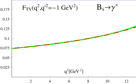
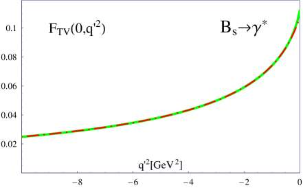
(a)	(b)

Fig. 2: Solid (green) line is the results of direct calculations of the form factor $F_{TV}(q^{2},q^{\prime 2})$ for $\lambda_{B_{s}}=0.6$ GeV. Dashed (red) line is the results of the double fit to $F_{TV}(q^{2},q^{\prime 2})$ in the range $-10<q^{\prime 2}({\rm GeV}^{2})<-0.6$ and $0<q^{2}({\rm GeV}^{2})<6$.

One can reach a much better accuracy (at a per mille level) if one proceeds in a bit different way: namely, performs a fit to the calculated $F_{TV}(q^{2},q^{\prime 2})$ in the single variable $q^{\prime 2}$ in the range $-10<q^{\prime 2}\;({\rm GeV}^{2})<-0.6$ for any fixed value of $q^{2}$ far below the quark threshold located at $(m_{b}+m_{s})^{2}$. We follow this route when calculating the dependence of $T_{1}(0)$ and $V(0)$ on $\lambda_{B_{s}}$ (see below).

As suggested by Eq. (2.9), in the region $0<q^{2}({\rm GeV}^{2})<6$ the results of our calculation may be well approximated by a simple monopole formula $F(q^{2})=F_{0}\left(1+a_{1}y_{1}/(1-y_{1})\right)$ with $y_{1}=q^{2}/M^{2}_{B_{s}^{*}}$.

2.3 Radiative corrections and constraints on $\lambda_{B_{s}}(\mu)$

It is time to recall that the analysis of the previous Section does not include the radiative corrections, whereas for the form factors of the tensor current, $F_{TV}(q^{2},q^{\prime 2})$ and $T_{1}(q^{2})$ which depend on the scale $\mu$, the radiative corrections are crucial for controlling this scale-dependence. Also for the form factors $F_{V}(q^{2},q^{\prime 2})$ and $V(q^{2})$, the radiative corrections may change the dependence of these form factors on $\lambda_{B_{s}}(\mu)$.

Two remarks are in order.

$\bullet$ The radiative corrections are known for the case $F_{V}(q^{2},q^{\prime 2}=0)$ as the function of $E_{\gamma}=(M_{B_{s}}^{2}-q^{2})/(2M_{B_{s}})$, see beneke2011 and Appendix B. The corresponding factor $R(E_{\gamma},\mu)$ is shown in Fig. 3 for $\mu=m_{b}$.

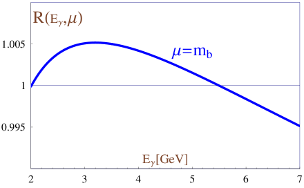
Fig. 3: The factor $R(E_{\gamma},\mu=m_{b})$ describing radiative corrections to the form factor $F_{V}(E_{\gamma})$.

As seen from this plot, the correction evaluated at $\mu=m_{b}$ is negligible in the range $2<E_{\gamma}({\rm GeV}^{2}<7$. Recall, however, that we have a different situation: namely, $q^{2}\neq 0$ and $q^{\prime 2}<0$. We now give arguments that the results for $F_{V}(q^{2},q^{\prime 2}=0)$ may be used to estimate the radiative corrections for $F_{V}(q^{2},q^{\prime 2})$ at $q^{\prime 2}<0$.

Let us introduce the “equivalent” energy $\bar{E}_{\gamma}(q^{2},q^{\prime 2})$ by the following expression:

$$m_{s}^{2}+M_{B_{s}}^{2}\bar{\xi}(1-\bar{\xi})-q^{2}\bar{\xi}-q^{\prime 2}(1-\bar{\xi})\equiv 2M_{B_{s}}\bar{\xi}\bar{E}_{\gamma}(q^{2},q^{\prime 2}),$$ (2.10)

such that the denominator in Eq. (2.1) at $\xi=\bar{\xi}$ gives $2M_{B_{s}}\bar{E}_{\gamma}\bar{\xi}$. Obviously, $\bar{E}_{\gamma}\to E_{\gamma}$ for $m_{s}\to 0$, $q^{\prime 2}\to 0$, and $\bar{\xi}\to 0$.

The behaviour of the form factor and of the radiative corrections are related to the behaviour of the denominator of Eq. (2.1). So, we expect that the radiative correction in $F_{V}(q^{2},q^{\prime 2})$ may be estimated using the function $R(\bar{E}_{\gamma},\mu)$ evaluated for $\bar{\xi}$, the value at which $\phi_{+}(\xi)$ reaches its maximum. For the 2DAs considered here one obtains $\bar{\xi}\simeq 0.2$, and it is easy to check that for the range used in our analysis, namely $-10<q^{\prime 2}({\rm GeV}^{2})<0$ and $0<q^{2}({\rm GeV}^{2})<6$, $\bar{E}_{\gamma}$ varies in the range $2<\bar{E}_{\gamma}({\rm GeV}^{2})<7$. Thus, for the analysis of the previous Section, the radiative corrections in the form factor $F_{V}$ are at the level of less than 1% and may be neglected, if one expresses the leading-order contribution to the form factor $F_{V}(q^{2},q^{\prime 2})$, Eq. (2.1), via $\lambda_{B_{s}}(\mu=m_{b})$.

$\bullet$ The radiative corrections for the form factor $F_{TV}(q^{2},q^{\prime 2})$ have not yet been calculated for any values of $q^{2}$ and $q^{\prime 2}$. Again, since the behaviours of the form factors and of the radiative correction are determined by the same denominator appearing in the analytic formulas for $F_{TV}(q^{2},q^{\prime 2})$ and $F_{V}(q^{2},q^{\prime 2})$, we conjecture that the radiative corrections at $\mu=m_{b}$ in the considered range of values of $q^{2}$ and $q^{\prime 2}$ may be neglected too.

Moreover, the form factors of the tensor current depend on the scale, in particular, one has $F_{TV}(0,0|\mu)$ and $T_{1}(0|\mu)$. Our arguments for a negligible size of the radiative corrections at $\mu=m_{b}$ imply that the analysis of the previous Section yields $F_{TV}(0,0|\mu=m_{b})$ and $T_{1}(0|\mu=m_{b})$ as soon as the leading-order contributions in $\alpha_{s}$, Eq. (2.1), are expressed via $\lambda_{B_{s}}(\mu=m_{b})$.

We would like to emphasize that for our extraction of $\lambda_{B_{S}}(\mu)$ it is not crucial that the radiative corrections vanish precisely at $\mu=m_{b}$; it is only important that these corrections vanish at $\mu\sim m_{b}$. We shall see later (Fig. 5) that the dependence of $\lambda_{B_{S}}(\mu)$ in the region $\mu\sim m_{b}$ is relatively flat and, therefore, the impact of the precise value of the scale at which the radiative corrections vanish, has only a moderate impact on, e.g., the extracted value of $\lambda_{B_{s}}(\mu=m_{b})$.

Fig. 4 presents the results based on Eqs. (2.1) showing strong correlations between the value of $\lambda_{B_{s}}\equiv\lambda_{B_{s}}(m_{b})$ and the form factor values $F_{V}(0,0)$, $V(0)$, $F_{TV}(0,0|\mu=m_{b})$ and $T_{1}(0|\mu=m_{b})$.

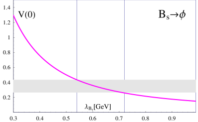
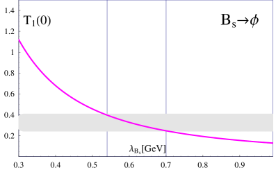
(a)	(b)
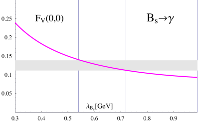
(c)	(d)

Fig. 4: (a) Form factor $V(0)$ calculated via the leading order diagram of Fig. 1 (a) vs $\lambda_{B_{s}}=\lambda_{B_{s}}(m_{b})$. The band covers the results for $V(0)$ in Table 2. (b) Form factor $T_{1}(0)$ at the scale $\mu=m_{b}$ calculated via the leading order diagram of Fig. 1 (a) vs $\lambda_{B_{s}}=\lambda_{B_{s}}(m_{b})$. The band covers the results for $T_{1}(0)$ in Table 2. (c) Form factor $F_{V}(0,0)$ vs $\lambda_{B_{s}}$. The band of values of $F_{V}(0,0)$ corresponds to the allowed band of $\lambda_{B_{s}}(m_{b})$ from Plot. (a) (d) Form factor $F_{TV}(0,0)$ at the scale $\mu=m_{b}$ vs $\lambda_{B_{s}}$. The band of values of $F_{TV}(0,0)$ corresponds to the allowed band of $\lambda_{B_{s}}(m_{b})$ from Plot. (b).

In order to disentangle the appropriate value of $\lambda_{B_{S}}(m_{b})$ we use the existing estimates of the $B_{s}\to\phi$ form factors $V(0)$ and $T_{1}(0|m_{b})$, obtained using approaches not directly referring to the 2DAs of $B_{s}$-meson.

Table 2: Theoretical results for the $B_{s}\to\phi$ form factors $V(0)$ and $T_{1}(0|\mu=m_{b})$ and the corresponding $\lambda_{B_{s}}(m_{b})$ obtained from Fig. 4.

	ms2000	ballbraun1998	ballzwicky2005	lattice2014	ivanov2016
$V(0)$	$0.44\pm 0.05$	$0.43\pm 0.06$	$0.433\pm 0.035$	$0.24\pm 0.07$	$0.31\pm 0.03$
$\lambda_{B_{s}}(\mu=m_{b})[{\rm GeV}]$	0.54	0.55	0.55	0.72	0.65
$T_{1}(0|\,\mu=m_{b})$	$0.38\pm 0.04$	$0.35\pm 0.05$	$0.349\pm 0.033$	$0.31\pm 0.02$	$0.27\pm 0.03$
$\lambda_{B_{s}}(\mu=m_{b})[{\rm GeV}]$	0.54	0.58	0.58	0.62	0.7

Table 2 shows a selection of such results obtained from quark models ms2000 ; ivanov2016 , light-cone QCD sum rules based on the $\phi$-meson DAs ballbraun1998 ; ballzwicky2005 , and lattice QCD lattice2014 .

Conservatively, the existing results provide the allowed range

$$V(0)=0.34\pm 0.10,\qquad T_{1}(0|\mu=m_{b})=0.32\pm 0.06.$$ (2.11)

Fig. 4(a) then yields the corresponding allowed range $\lambda_{B_{S}}(m_{b})=(0.62\pm 0.10)$ GeV and from Fig. 4(b) one obtains the estimate for the $B_{s}\to\gamma$ form factors $F^{(s)}_{V}(0,0)=0.13\pm 0.01$ and $F^{(s)}_{TV}(0,0|m_{b})=0.105\pm 0.015$. These values are in agreement with the estimate obtained in mnk2018 , $F^{(s)}_{V}(0,0)=0.1$ and $F^{(s)}_{TV}(0,0|m_{b})=0.11$, and consistent also with the recent lattice QCD calculations of lattice2024 .

Making use of the results for $R(q^{2}=0,\mu)$ from Appendix A (Fig. 5(a)) and the property that $R(q^{2}=0,\mu)/\lambda_{B_{s}}(\mu)$ is scale-independent, we obtain the $\mu$-dependence of $\lambda_{B_{s}}(\mu)$ shown in Fig. 5. Evolving the allowed range of $\lambda_{B_{s}}(\mu)$ from $\mu=m_{b}$ to $\mu\simeq 1$ GeV, we obtain the estimate

$$\lambda_{B_{s}}(1\mbox{ GeV})=0.49\pm 0.07\mbox{ GeV}.$$ (2.12)

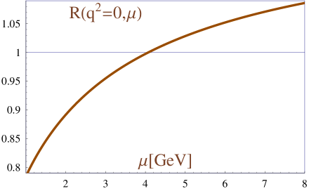
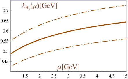
(a)	(b)

Fig. 5: (a) The dependence of the factor $R(0,\mu)$ on $\mu$. (b) The dependence of $\lambda_{B_{s}}(\mu)$ on $\mu$. Solid line describes the evolution of the central value of the allowed interval of $\lambda_{B_{s}}(m_{b})$ whereas the dash-dotted lines correspond to the lower and the upper boundaries of the allowed interval of $\lambda_{B_{s}}(m_{b})$.

3 Discussion and conclusions

A. We have formulated an efficient algorithm of obtaining the form factors $F_{V,TV}(q^{2},q^{\prime 2})$ in a broad range of momentum transfers including the region of meson resonances where the form factors cannot be calculated using finite-order QCD diagrams. Our algorithm is based on the following steps:

i. We calculate the form factors $F_{V,TV}(q^{2},q^{\prime 2})$ at the lowest order in $\alpha_{s}$ via the 2DAs of the $B_{s}$ meson in a broad range of $q^{2}$ and $q^{\prime 2}$ far below quark thresholds where the calculation based on finite order Feynman diagrams may be trusted. In this way we obtain, in particular, the dependence of $F_{V,TV}(q^{2},q^{\prime 2})$ on the parameter $\lambda_{B_{s}}$ making use of the lowest order in $\alpha_{s}$.

ii. We interpolate the obtained results by an analytic formula based on dispersion representation for $F_{V,TV}(q^{2},q^{\prime 2})$ in $q^{\prime 2}$ with one subtraction. The considered analytic formula takes into account the presence of the $\phi$-meson pole in the physical form factor and takes into account contribution of the excited hadron states via an effective pole whose mass and coupling are fitting parameters.

iii. We obtain predictions for the form factors $F_{V}(q^{2},q^{\prime 2})$ and $F_{TV}(q^{2},q^{\prime 2})$ in the physical region by using the fitting formula in a broad range of momentum transfers including the resonance region.

B. We applied this algorithm and obtained the $B_{s}\to\phi$ form factors $V(q^{2})$ ($T_{1}(q^{2})$) as a residue of $F_{V}(q^{2},q^{\prime 2})$ ($F_{TV}(q^{2},q^{\prime 2})$) of the pole located at $q^{\prime 2}=M_{\phi}^{2}$ without using QCD sum rules. In this way we avoid the systematic uncertainties related to the method of QCD sum rules which are not possible to control in a rigorous way lms2007a ; lms2007b ; lms2009a ; lms2009b ; m2009 .

C. Our analysis is based on the correlation function calculated at leading order in $\alpha_{s}$. Making use of the fact that the radiative corrections for the form factor $F_{V}(q^{2},q^{\prime 2}=0)$ evaluated at the scale $\mu=m_{b}$ turn out to be small in a broad range of photon energies $E_{\gamma}$, we have given arguments that the same property is valid for the form factors $F_{V}(q^{2},q^{\prime 2})$ in a broad range of values of $q^{2}$ and $q^{\prime 2}$ far below the quark thresholds, where our fitting procedure is carried out. In the case of the form factor $F_{TV}(q^{2},q^{\prime 2})$ the radiative corrections are not known at all, but also in this case we may conjecture that the same property is valid.

We emphasize that it is not necessary that the radiative corrections vanish precisely at the scale $\mu=m_{b}$; it is sufficient that they vanish at some scale not far from $m_{b}$. Then, the obtained estimate for $\lambda_{B_{s}}(\mu=m_{b})$ would change only marginally as the dependence of $\lambda_{B_{s}}(\mu)$ in the region $\mu\sim m_{b}$ is relatively flat. But, obviously, for putting our analysis on a solid theoretical basis, a direct evaluation of the radiative corrections for the form factors of the tensor currents would be crucial.

Given the property that the radiative corrections are small at $\mu=m_{b}$, our leading-order expressions for the form factors evaluated via the 2DAs at the scale $\mu=m_{b}$, containing $\lambda_{B_{s}}(m_{b})$, should provide a good approximation for the form factors $F_{V}(q^{2},q^{\prime 2})$ and $V(q^{2})$ as well as for $F_{TV}(q^{2},q^{\prime 2}|\mu=m_{b})$ and $T_{1}(q^{2}|\mu=m_{b})$.

Then, having at hand the dependence of $T_{1}(0)$ and $V(0)$ on $\lambda_{B_{s}}(m_{b})$ and making use of the theoretical results for $B_{s}\to\phi$ form factors $V(0)$ and $T_{1}(0|\mu=m_{b})$, obtained by approaches which do not use the 2DAs of $B_{s}$-meson, we extract the following allowed range s

$$\lambda_{B_{s}}(\mu\simeq m_{b})=0.62\pm 0.10\mbox{ GeV}~{},~{}$$ (3.13)

$$\lambda_{B_{s}}(1\mbox{ GeV})=0.49\pm 0.07\mbox{ GeV}.$$ (3.14)

The latter result agrees nicely with thea recent estimate $\lambda_{B_{s}}(1\mbox{ GeV})=0.48\pm 0.09$ GeV obtained using QCD sum rules in lambdabs2024 .

Closing this paper, we believe that the proposed method for extracting the meson-to-meson transition form factor as a residue of a dominant pole, like $T_{1}(q^{2})$ in the form factor $F_{TV}(q^{2},q^{\prime 2})$, may be promising for calculating other meson transition form factors and may be used as a complementary method to QCD sum rules.

Appendix A Form factor $T_{1}(q^{2})$ for $B_{s}\to\phi$ from QCD sum rule

Here we would like to recall briefly a sum-rule calculation of the form factor $T_{1}(q^{2})$. The starting point is the same correlation function (2.2) and the form factor $F_{TV}(q^{2},q^{\prime 2})$. Eq. (2.4) based on the calculation of QCD diagrams, may be identically rewritten in the form of a dispersion representation in $q^{\prime 2}$:

$$F_{TV}(q^{2},q^{\prime 2})=\int\limits_{0}^{2\omega_{0}}d\xi\frac{\phi_{B_{s}}(\xi)}{1-\xi}\int ds^{\prime}\frac{1}{s^{\prime}-q^{\prime 2}}\delta\left(s^{\prime}-\frac{m_{s}^{2}+\xi(1-\xi)M_{B_{s}}^{2}-q^{2}\xi}{1-\xi}\right),$$ (A.15)

where we introduce a short-hand notation

$$\phi_{B_{s}}(\xi)\equiv-Q_{s}M_{B_{s}}f_{B_{s}}\left[\phi_{+}(\xi)(1-\xi)+\bar{\Phi}(\xi)\right].$$ (A.16)

We can now make a subtraction in this spectral representation and write:

$$F_{TV}(q^{2},q^{\prime 2})=F_{TV}(q^{2},0)+q^{\prime 2}\int\limits_{0}^{2\omega_{0}}d\xi\frac{\phi_{B_{s}}(\xi)}{1-\xi}\int ds^{\prime}\frac{1}{s^{\prime}(s^{\prime}-q^{\prime 2})}\delta\left(s^{\prime}-\frac{m_{s}^{2}+\xi(1-\xi)M_{B_{s}}^{2}-q^{2}\xi}{1-\xi}\right).$$ (A.17)

Obviously, the representation (A.15) may not be used in the region of $q^{\prime 2}$ close to the quark threshold at $4m_{s}^{2}$. On the other hand, from the general property of the correlation function, $F_{TV}(q^{2},q^{\prime 2})$ contains a pole at $q^{\prime 2}=M_{\phi}^{2}$.

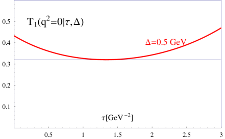
Fig. 6: The dual form factor $T_{1}(0|\tau,\Delta)$, a QCD sum rule estimate for $T_{1}(0)$; $\Delta=0.5$ GeV.

We can now equate to each other two different representations for $F_{TV}(q^{2},q^{\prime 2})$ – the phenomenological side of a QCD sum rule (in the language of hadron states) and the theoretical side (based on QCD diagrams):

$$F_{TV}(q^{2},q^{\prime 2}) = R_{\phi}T_{1}(q^{2})\frac{1}{M_{\phi}^{2}-q^{\prime 2}}+\ldots$$ (A.18)

$$= F_{TV}(q^{2},0)+q^{\prime 2}\int\limits_{0}^{1}d\xi\frac{\phi_{B_{s}}(\xi)}{1-\xi}\int ds^{\prime}\frac{1}{s^{\prime}(s^{\prime}-q^{\prime 2})}\delta\left(s^{\prime}-\frac{m_{s}^{2}+\xi(1-\xi)M_{B_{s}}^{2}-q^{2}\xi}{1-\xi}\right),$$

where $\dots$ denote the contribution of hadron continuum and the excited resonances. To isolate the pole at $q^{\prime 2}=M_{\phi}^{2}$ we perform two standard steps adopted in QCD sum rules:

• Introduce the effective threshold $s_{\rm eff}$ and apply the duality cut $s^{\prime}<s_{\rm eff}$. We shall make use of the standard hypothesis (“Braun prescription”) based on the properties of hadron spectrum:

  $$s_{\rm eff}=(M_{\phi}+\Delta)^{2},\quad\Delta\simeq 500\;{\rm MeV}.$$ (A.19)

• Perform Borel transform $q^{\prime 2}\to\tau$ $(\equiv 1/M_{\rm Borel}^{2})$:

  $$1/(s^{\prime}-q^{\prime 2})\to\exp(-s^{\prime}\tau),\quad 1/(M_{\phi}^{2}-q^{\prime 2})\to\exp(-M_{\phi}^{2}\tau).$$ (A.20)

  This Borel transform suppresses the contributions of higher-mass resonances on the phenomenological side of the QCD sum rule for $F_{TV}(q^{2},q^{\prime 2})$ and kills all polynomial terms in $q^{\prime 2}$ on the OPE side of the QCD sum rule, including possible subtraction terms.

Using the $\delta$-function to take the $s^{\prime}-$integral, we obtain the dual form factor $T_{1}(q^{2}|\tau,\Delta)$ from which one should obtain a sum-rule estimate for the physical form factor $T_{1}(0)$:

$$T_{1}(q^{2}|\tau,\Delta)=\frac{1}{R_{\phi}}\int\limits_{0}d\xi\frac{\phi_{B_{s}}(\xi)}{1-\xi}\exp\left[\tau\left(M_{\phi}^{2}-\frac{m_{s}^{2}+\xi(1-\xi)M_{B_{s}}^{2}-q^{2}\xi}{1-\xi}\right)\right]\theta\left(\frac{m_{s}^{2}+\xi(1-\xi)M_{B_{s}}^{2}-q^{2}\xi}{1-\xi}\leq s_{\rm eff}\right).$$ (A.21)

Note that the actual upper limit of the $\xi$-integration in Eq. (A.21) is determined by the $\theta$-function (and not by the parameter $2\omega_{0}$ expected to be of the order of $\sim 0.5$) leaving the $\xi$-integration region in the dual form factor closer to zero, i.e. $\xi\leq s_{\rm eff}/M_{B_{s}}^{2}\sim 0.1$.

The dual form factor contains two auxiliary parameters, the effective threshold $\Delta$ and the Borel parameter $\tau$. We shall not try to play the game with stability windows but just fix $\Delta$ as mentioned above and take the minimal value in the Borel window as the SR estimate for the form factor $T_{1}(0)$. This gives $T_{1}(0)\simeq 0.32$ (see Fig. 6).

Appendix B Radiative corrections to the form factor $F_{V}$

The radiative corrections for the tensor current form factors $F_{TV,TA}$ are not known. We therefore refer to the known radiative corrections for the form factors $F_{A,V}$ beneke2011 . The necessary formulas from beneke2011 are reproduced here for the convenience of the reader.

To the leading order in $1/m_{b}$, the form factors $F_{A,V}$ have the following behaviour:

$$F_{A,V}(E_{\gamma}) = \frac{Q_{u}M_{B_{s}}f_{B_{s}}}{2E_{\gamma}\lambda_{B_{s}}(\mu)}\,R(E_{\gamma},\mu)+\dots$$ (B.22)

The factor $R(E_{\gamma},\mu)$ describing the radiative corrections can be written as a product of several factors,

$$R(E_{\gamma},\mu)=C(E_{\gamma},\mu_{h1})K^{-1}(\mu_{h2})\times U(E_{\gamma},\mu_{h1},\mu_{h2},\mu)\times J(E_{\gamma},\mu),$$ (B.23)

which come from the different scales contributing to the process, namely:

$\bullet$ the factor relating the decay constant of the $B$-meson in QCD and HQET

$$K(\mu)=1+\frac{\alpha_{s}C_{F}}{4\pi}\left(\frac{3}{2}\ln\frac{m_{b}^{2}}{\mu^{2}}-2\right).$$ (B.24)

$\bullet$ the factor related to the matching between the weak currents in QCD and SCET

$$C(E_{\gamma},\mu)=1+\frac{\alpha_{s}C_{F}}{4\pi}\left(-2\ln^{2}\frac{2E_{\gamma}}{\mu}+5\ln\frac{2E_{\gamma}}{\mu}-\frac{3-2x}{1-x}\ln x-2{\rm Li}_{2}(1-x)-6-\frac{\pi^{2}}{12}\right),\quad x=2E_{\gamma}/m_{b}.$$ (B.25)

$\bullet$ the hard-collinear radiative correction

$$J(E_{\gamma},\mu)=1+\frac{\alpha_{s}C_{F}}{4\pi}\left(\ln^{2}\frac{2E_{\gamma}\mu_{0}}{\mu^{2}}-2\sigma_{1}(\mu,\mu_{0})\ln\frac{2E_{\gamma}\mu_{0}}{\mu^{2}}-1-\frac{\pi^{2}}{6}+\sigma_{2}(\mu,\mu_{0})\right)$$ (B.26)

with the inverse-logarithmic moments defined as

$$\frac{1}{\lambda_{B_{s}}(\mu)}=\int_{0}^{\infty}\frac{d\omega}{\omega}\,\phi_{+}(\omega,\mu),\qquad\sigma_{n}(\mu,\mu_{0})=\lambda_{B_{s}}(\mu)\int_{0}^{\infty}\frac{d\omega}{\omega}\,\ln^{n}\frac{\mu_{0}}{\omega}\,\phi_{+}(\omega,\mu)$$ (B.27)

where $\mu_{0}=1\mbox{ GeV}$ is a fixed reference scale which is part of the definition of the inverse-logarithmic moments adopted in beneke2011 . Parameter $\omega$ in (B.26) is related to dimensionless parameter $\xi$ in (2.6) as $\omega=M_{B_{s}}\xi$.

In beneke2011 the authors notice the absence of a common scale $\mu$ that avoids parametrically large logarithms of order $\ln m_{b}/\mu_{0}$ in (B.24), (B.25) and (B.26) and introduce the evolution factor $U(E_{\gamma},\mu_{h1},\mu_{h2},\mu)$ into (B.23). Its explicit expression is given in the Appendix of beneke2011 .

Our observation based on the above formulas and on the explicit form of the 2DAs is however a bit different from the conclusion of beneke2011 . Indeed, for the 2DA of the LD model (2.6), the dependence of $J(E_{\gamma},\mu)$ in (B.26) on $\mu_{0}$ drops out. We have checked that this property holds as well also for a different 2DA model referred to as Model IIA in braun2017 . Thus, we expect that, at least at order ${\cal{O}}(\alpha_{s})$, the factor $J(E_{\gamma},\mu)$ of $\mu_{0}$ is independent of $\mu_{0}$.

Because of this property, one can set $\mu_{0}$ equal to the hard scale $\mu$ thus avoiding large logs in all three factors (B.24), (B.25) and (B.26). In this case, the expressions (2.13) and (2.14) from beneke2011 and the expressions (42) and (43) from braun2004 (correspond to setting $\mu_{0}\to\mu$) lead to the same results. If so, one can choose the common hard scale in all factors (B.24), (B.25) and (B.26), and the evolution factor $U(E_{\gamma},\mu_{h1},\mu_{h2},\mu)$ reduces to unity.

Moreover, at the scale $\mu=m_{b}$, the factor $R(E_{\gamma},\mu=m_{b})$ is very close to unity in a broad range of values of $q^{2}$. Therefore, for $\mu=m_{b}$ the radiative corrections may be neglected and the leading-order analysis is expected to provide reliable results.

References

- (1) G. P. Korchemsky, D. Pirjol, and T.-M. Yan, Radiative leptonic decays of B mesons in QCD, Phys. Rev. D61, 114510 (2000).
- (2) V. Braun, Y. Ji, and A. Manashov, Higher-twist B-meson Distribution Amplitudes in HQET”, JHEP 05, 022 (2017).
- (3) M. Beneke, C. Bobeth and Y.-M. Wang, decay with an energetic photon, JHEP 12, 148 (2020).
- (4) I. Belov, A. Berezhnoy, and D. Melikhov, Charming-loop contributions in decays, Phys. Rev. D108, 094007 (2023).
- (5) I. Belov, A. Berezhnoy, and D. Melikhov, Nonfactorizable charming-loop contribution to FCNC decay, Phys. Rev. D109, 114012 (2024).
- (6) Y.-K. Huang, Y. Ji, Y.-L. Shen, C. Wang, Y.-M. Wang, X.-C. Zhao, Renormalization-Group Evolution for the Bottom-Meson Soft Function, e-Print: 2312.15439 [hep-ph].
- (7) P. Ball and E. Kou, transitions from QCD sum rules on the light cone, JHEP 0304, 029 (2003).
- (8) V. M. Braun, D. Yu. Ivanov, and G. P. Korchemsky. The B meson distribution amplitude in QCD, Phys. Rev. D69 034014 (2004).
- (9) M. Beneke and J. Rohrwild, B meson distribution amplitude from , Eur. Phys. J. C71, 1818 (2011).
- (10) Y. M. Wang, Factorization and dispersion relations for radiative leptonic decay, JHEP 09, 159 (2016).
- (11) T. Janowski, B. Pullin, and R. Zwicky, Charged and neutral form factors from light cone sum rules at NLO, JHEP 12, 008 (2021).
- (12) M. A. Ivanov and D. Melikhov, Theoretical analysis of the leptonic decay , Phys. Rev. D105, 014028 (2022); Phys. Rev. D106, 119901(E) (2022).
- (13) A. Khodjamirian, R. Mandal, and T. Mannel, Inverse moment of the -meson distribution amplitude from QCD sum rule, JHEP 10, 043 (2020).
- (14) F. Kruger and D. Melikhov, Gauge invariance and form-factors for the decay , Phys. Rev. D67, 034002 (2003).
- (15) A. Kozachuk, D. Melikhov, and N. Nikitin, Rare FCNC radiative leptonic decays in the Standard Model, Phys. Rev. D97, 053007 (2018).
- (16) D. Melikhov, O. Nachtmann, V. Nikonov, and T. Paulus, Masses and couplings of vector mesons from the pion electromagnetic, weak, and transition form-factors, Eur. Phys. J. C34, 345 (2004).
- (17) V. M. Braun and I. Halperin, Soft contribution to the pion form-factor from light cone QCD sum rules, Phys. Lett. B328, 457 (1994).
- (18) A. Khodjamirian, T. Mannel, and N. Offen, Form-factors from light-cone sum rules with B-meson distribution amplitudes, Phys. Rev. D75, 054013 (2007).
- (19) M. Ivanov, D. Melikhov, and S. Simula, Form factors for decays into two currents in QCD, Phys. Rev. D101, 094022 (2020).
- (20) D. Melikhov and B. Stech, Weak form-factors for heavy meson decays: an update, Phys. Rev. D62, 014006 (2000).
- (21) P. Ball and V. M. Braun, Exclusive semileptonic and rare B meson decays in QCD, Phys. Rev. D58, 094016 (1998).
- (22) P. Ball and R. Zwicky, decay form factors from light-cone sum rules reexamined, Phys. Rev. D71, 014029 (2005).
- (23) R. Horgan, Z. Liu, S. Meinel, and M. Wingate, Lattice QCD calculation of form factors describing the rare decays and , Phys. Rev. D89, 094501 (2014).
- (24) S. Dubnička, A. Z. Dubničková, A. Issadykov, M. A. Ivanov, A. Liptaj and S. K. Sakhiyev, Decay in covariant quark model, Phys. Rev. D93, 094022 (2016).
- (25) R. Frezzotti, G. Gagliardi, V. Lubicz, G. Martinelli, C. T. Sachrajda et al, The decay rate at large from lattice QCD, e-Print: 2402.03262 [hep-lat]
- (26) W. Lucha, D. Melikhov, and S.Simula, Systematic uncertainties of hadron parameters obtained with QCD sum rules, Phys. Rev. D76, 036002 (2007).
- (27) W. Lucha, D. Melikhov, and S. Simula, Can one control systematic errors of QCD sum rule predictions for bound states?, Phys. Lett. B657, 148 (2007).
- (28) W. Lucha, D. Melikhov, H. Sazdjian, and S. Simula, Effective continuum threshold for vacuum-to-bound-state correlators, Phys. Rev. D80, 114028 (2009).
- (29) W. Lucha, D. Melikhov, and S. Simula Accuracy of bound-state form factors extracted from dispersive sum rules, Phys. Lett. B671, 445 (2009).
- (30) D. Melikhov, Hadron form factors from sum rules for vacuum-to-hadron correlators, Phys. Lett. B671, 450 (2009).
- (31) R. Mandal, P. S Patil, and I. Ray, Probing the inverse moment of -meson distribution amplitude via form factors, arXiv:2402.16737.