Anisotropic cosmology in Bumblebee gravity theory
Abstract
The Bumblebee vector model of spontaneous Lorentz symmetry breaking (LSB) in Bianchi type I (BI) Universe to observe its effect on cosmological evolution is an interesting aspect of study in anisotropic cosmology. In this study, we have considered a Bumblebee field under vacuum expectation value condition (VEV) with BI metric and studied the cosmological parameters along with observational data. Further, we have studied the effect of anisotropy and the Bumblebee field in cosmic evolution. We have also studied the effect of both anisotropy and Bumblebee field while considering the Universe as a dynamical system. We have found that there are some prominent roles of both anisotropy and the Bumblebee field in cosmic evolutions. We have also observed an elongated matter-dominated phase as compared to standard cosmology. Moreover, while studying the dynamical system analysis, we have also observed the shift of critical points from standard CDM results showing the anisotropy and the Bumblebee field effect.
I Introduction
Standard cosmology, also known as CDM cosmology mainly relies on the two cosmological principles, viz., the isotropy and the homogeneity of the Universe on a large scale. Along with the Friedmann-Lemaître-Robertson-Walker (FLRW) metric supported by an energy-momentum tensor of conventional perfect fluid form, this theory provides answers to many questions regarding the understanding of the Universe [1]. However, the observed accelerated expansion of the Universe [2, 3, 4] along with the absence of observational evidence on the dark matter (DM) [5] and dark energy (DE) [6] etc. have motivated researchers to search for alternate theories or modifications in general relativity (GR) through expanding the conventional formalism [7]. In this context, a gravitational model known as the Bumblebee gravity model was proposed [8]. This model is beyond the ambit of GR, which relaxes the cosmological principles. In this theory, a vector field known as the Bumblebee field has been introduced and as a result, it modifies the Einstein field equations of GR.
The Bumblebee model was first introduced in 1989 by Kostelecky and Samuel [8]. This is a simple yet reliable standard model extension (SME) that basically works in the principle of Lorentz symmetry breaking (LSB) [8, 9] through using a vector field. The model introduces this field and the potential in the conventional Einstein-Hilbert (EH) action which results in the modification of the general Einstein field equations and it helps to understand the various cosmological aspects without considering the exotic matter and energy contents like DM and DE in the Universe [7, 10]. However, several other SMEs are also available, in which the EH action was modified through the inclusion of some nontrivial curvature terms [11, 12], suitable scalar terms [13], vector fields [14, 15, 16] and so on. The impact of SMEs in the research of the gravitational sector can be found in the Refs. [17, 18, 20, 21, 19, 22, 23].
Although, as mentioned already, the isotropic and homogeneous cosmology successfully explains most of its aspects with the help of the standard CDM model which includes the Hubble tension [24, 25], the tension [24], the coincidence problem [26] etc., several dependable observational data sources, including WMAP [27, 28, 29], SDSS (BAO) [30, 31, 32], and Planck [33, 24] have shown some deviations from the principles of standard cosmology. These suggest that the Universe may have some anisotropies. Additionally, some studies have pointed to a large-scale planar symmetric geometry of the Universe, and for such a geometry the eccentricity of the order can match the quadrupole amplitude to the observational evidence without changing the higher-order multipole of the temperature anisotropy in the CMB angular power spectrum [34]. Again, the existence of asymmetry axes in the vast scale geometry of the Universe is also evident from the polarization analysis of electromagnetic radiation which is traveling across great cosmological distances [35]. Thus, the isotropy and homogeneity assumptions are not sufficient to explain all the cosmological phenomena completely. To explain these anisotropies, we require a metric with a homogeneous background that possesses the anisotropic character. Such a class of metrics had already been provided by Luigi Bianchi and out of his eleven types of metrics, Bianchi type I (BI) is the simplest yet suitable to explain the anisotropy of the Universe [36]. Researchers have already used this metric along with its special case like the locally rotationally symmetric BI (LRS-BI) metric to explain different aspects of anisotropic cosmology in both GR and other modified theories and some of them are found in the Refs. [37, 38, 39, 40, 41, 42, 43, 44, 45, 36, 46, 47, 48].
The SME theory of the Bumblebee vector field has been extensively studied by researchers in the black hole physics [22, 23, 49, 50, 51]. However, there are very limited studies that have been carried out on cosmological scenarios. Cosmological implications of Bumblebee theory on isotropic cosmology can be found in the Refs. [7, 14]. In anisotropic cosmology too the study of Bumblebee gravity is in the very preliminary stage. In Ref. [52], the Bumblebee field is considered as a source of cosmological anisotropies. Another work of Bumblebee gravity on the Kesner metric has been found in Ref. [53]. However, constraining the model parameters with the help of various observational data and extensive studies of cosmological parameters in Bumblebee gravity with Bianchi type I metric is an interesting topic of study to understand the Universe as well as the role of anisotropy and Bumblebee field in cosmic expansion and evolution.
In this work, we have considered the BI metric along with the Bumblebee vector model to explain the anisotropic characteristics of the Universe by studying the cosmological parameters. Here we have used available observational data like Hubble data, Pantheon data, BAO data, etc. to understand the situation in a more realistic and physical way. Further, we have covered the study of the effect of anisotropy and Bumblebee field on cosmic evolution through the study of the evolution of the density parameters against cosmological redshift. Finally, we have also studied the dynamical system analysis for the considered case to understand the property of the critical points and sequences of the evolution of the various phases of the Universe. In all our analyses, we have compared our results with standard CDM results to understand the effect of anisotropy and Bumblebee field in cosmic expansion.
The current article is organized as follows. Starting from this introduction part in Section I, we have discussed the general form of field equations in the Bumblebee field in Section II. In Section III, we have developed the field equations and continuity equation for the Bianchi type I metric with the consideration of the time-dependent Bumblebee field. In Section IV, we have further simplified the situation by considering the vacuum expectation value (VEV) condition and derived the field equations and cosmological parameters. In Section V, we have constrained the model parameters by using the techniques of Bayesian inference by using various observational data compilations and compared our model results with standard cosmology by using the constrained values of the parameters. In Section VI, we have studied the effect of anisotropy and Bumblebee field on cosmological evolutions. In Section VII we have made the dynamical system analysis for both standard CDM and anisotropic Bumblebee model. Finally, the article has been summarised with conclusions in Section VIII.
II The Bumblebee gravity and field equations
The Bumblebee vector field model and its associated gravity theory are based on the principle of spontaneous Lorentz symmetry breaking (LSB) within the gravitational context. These models contain a potential term that, for the field configurations, results in nontrivial VEVs. This can have an impact on other fields’ dynamics that are coupled to the Bumblebee field, while also maintaining geometric structures and conservation laws that are compatible with the standard pseudo-Riemannian manifold used in GR [16, 17]. The simplest model with a single Bumblebee vector field coupled to gravity in a non torsional spacetime can be described by the action [7, 52],
| (1) |
where , is the coupling constant with the dimension of accounting for the interaction between the Bumblebee field and Ricci tensor of spacetime, is the Bumblebee vector field, is the field strength tensor, and is the matter Lagrangian density. Further, is the expectation value for the contracted Bumblebee vector field and is a field potential satisfying the condition: . The field equations obtained through varying the action (1) with respect to the metric can be written as
| (2) |
Here, is the Einstein tensor and is the energy momentum tensor. Further, varying the action (1) concerning the Bumblebee field gives the equation of motion of the field as [7, 52]
| (3) |
If the left-hand side of the equation (3) vanishes, then the relation becomes a simple algebraic relation between the Bumblebee potential and the geometry of spacetime. In our work, we have considered the Bianchi type I metric and a Bumblebee field to solve the equation (II). Here, we have considered the VEV of the field and hence it holds the condition: .
III Bianchi Cosmology in Bumblebee gravity
We have considered the Bianchi type I metric in our study which has the form:
| (4) |
where are the directional scale factors along directions respectively. Thus, BI metric provides three directional Hubble parameters: and along three axial directions. Accordingly, the average expansion scale factor for the metric is and the average Hubble parameter can be written as
| (5) |
In our work, we have considered the Bumblebee field, which has only one surviving component, the temporal component [7], i.e.
| (6) |
and it holds the condition, . Thus, under this condition equation (3) can be simplified as
| (7) |
Now, for the stress-energy tensor , the temporal component of the field equation (II) can be written as
| (8) |
And, the spatial components of the filed equations are obtained as follows:
| (9) |
| (10) |
| (11) |
Further, by adding all the spatial components of the field equations, one can write,
| (12) |
These equations are used later for deriving various cosmological parameters. Moreover, using the condition , we get the continuity relation as
| (13) |
IV Field Equations Under Vacuum Expectation Value (VEV) Condition
At VEV, the Bumblebee field equation holds the condition and also it can be assumed that the bumblebee field is constant for a time-like vector and gives the relation [53]. Thus, at VEV, while considering the average Hubble parameter expression (5), the field equations (8) and (III) can be written as
| (14) | ||||
| (15) |
Here, is the Lorentz violation parameter and
| (16) |
is the shear scalar associated with the anisotropic spacetime. Using equations (14) and (15) we can obtain the effective equation of state and it takes the form:
| (17) |
In terms of , the deceleration parameter can be written as
| (18) |
The continuity relation (III) under the VEV condition takes the form:
| (19) |
Now, taking the condition [46, 47] in which the is the expansion scalar, we can write, and , where and are two proportionality constants. These lead to the average Hubble parameter to have a simplified form in terms of the x-directional parameter as
| (20) |
and also lead to the shear scalar in form as
| (21) |
where and . In view of this form of , equation (IV) takes the form:
| (22) |
where . With the consideration of along with equations (14) and (15), the above equation can further be rewritten as
| (23) |
This equation of continuity can be solved for the density as
| (24) |
where
| (25) |
Furthermore, from the equation (14) we can write the Hubble parameter as
| (26) |
Again, taking the relation in which is the cosmological redshift, we can rewrite the Hubble parameter in the form:
| (27) |
where
| (28) |
with
| (29) |
| (30) |
| (31) |
Utilizing the expression of , i.e. , the distance modulus can be obtained from the following formula:
| (32) |
where is the luminosity distance and it has the mathematical form:
| (33) |
Also, the equation (17) for the effective equation of state can be rewritten as
| (34) |
With all these derivations, we are ready for the graphical visualization of all the cosmological parameters that have been expressed in equations (18), (27), (32) and (34). However, before doing that, we need to constrain different model parameters, like , etc. to obtain results consistent with the current observations which we have done in the next section.
V Parameters estimations and constraining
For estimating and constraining the parameters, we have used the Bayesian inference technique which is based on Bayes’ theorem. The theorem states that the posterior distribution of the parameter for the model with cosmological data can be obtained as
| (35) |
Here, , and are the likelihood, the prior probability of the model parameters and the Bayesian evidence respectively. The Bayesian evidence can be obtained as
| (36) |
in which the likelihood can be considered as a multivariate Gaussian likelihood function and it takes the form [45]:
| (37) |
where is the Chi-squared function of the dataset . For a uniform prior distribution of the model parameters, we can simply be considered the posterior distribution as
| (38) |
We have used this technique to estimate various model and cosmological parameters with the help of various observational data sets in our current work.
V.1 Data and their respective likelihoods
Here we will use observational data of Hubble parameter, BAO, CMB, and Pantheon supernovae type Ia from various sources to carry forward our analysis.
V.1.1 Hubble parameter
We have considered observational data from different literatures and tabulated them in Table 1. The chi-square function value for the mentioned dataset of denoted by can be calculated as
| (39) |
where is the standard deviation of the nth observational data and is the theoretical value of obtained from the considered cosmological model at .
| Reference | Reference | ||||
|---|---|---|---|---|---|
| 0.0708 | 69.0 19.68 | [54] | 0.48 | 97.0 62.0 | [64] |
| 0.09 | 69.0 12.0 | [55] | 0.51 | 90.8 1.9 | [61] |
| 0.12 | 68.6 26.2 | [54] | 0.52 | 94.35 2.64 | [59] |
| 0.17 | 83.0 8.0 | [55] | 0.56 | 93.34 2.3 | [59] |
| 0.179 | 75.0 4.0 | [56] | 0.57 | 92.4 4.5 | [65] |
| 0.199 | 75.0 5.0 | [56] | 0.57 | 87.6 7.8 | [66] |
| 0.20 | 72.9 29.6 | [54] | 0.59 | 98.48 3.18 | [59] |
| 0.24 | 79.69 2.65 | [57] | 0.593 | 104.0 13.0 | [56] |
| 0.27 | 77.0 14.0 | [55] | 0.60 | 87.9 6.1 | [63] |
| 0.28 | 88.8 36.6 | [54] | 0.61 | 97.8 2.1 | [61] |
| 0.30 | 81.7 6.22 | [58] | 0.64 | 98.82 2.98 | [59] |
| 0.31 | 78.18 4.74 | [59] | 0.6797 | 92.0 8.0 | [56] |
| 0.34 | 83.8 3.66 | [57] | 0.73 | 97.3 7.0 | [64] |
| 0.35 | 82.7 9.1 | [60] | 0.781 | 105.0 12.0 | [56] |
| 0.352 | 83.0 14.0 | [56] | 0.8754 | 125.0 17.0 | [56] |
| 0.36 | 79.94 3.38 | [59] | 0.88 | 90.0 40.0 | [64] |
| 0.38 | 81.9 1.9 | [61] | 0.90 | 117.0 23.0 | [55] |
| 0.3802 | 83.0 13.5 | [62] | 1.037 | 154.0 20.0 | [56] |
| 0.40 | 82.04 2.03 | [59] | 1.30 | 168.0 17.0 | [55] |
| 0.40 | 95.0 17.0 | [55] | 1.363 | 160.0 33.6 | [67] |
| 0.4004 | 77.0 10.2 | [62] | 1.43 | 177.0 18.0 | [55] |
| 0.4247 | 87.1 11.2 | [62] | 1.53 | 140.0 14.0 | [55] |
| 0.43 | 86.45 3.68 | [57] | 1.75 | 202.0 40.0 | [55] |
| 0.44 | 82.6 7.8 | [63] | 1.965 | 186.5 50.4 | [67] |
| 0.44 | 84.81 1.83 | [59] | 2.30 | 224 8.6 | [68] |
| 0.4497 | 92.8 12.9 | [62] | 2.33 | 224 8 | [69] |
| 0.47 | 89.0 50.0 | [64] | 2.34 | 223.0 7.0 | [70] |
| 0.4783 | 80.9 9.0 | [62] | 2.36 | 227.0 8.0 | [71] |
| 0.48 | 87.79 2.03 | [59] |
V.1.2 BAO measurements
Baryon acoustic oscillation (BAO) helps to understand the angular diameter distance between two points in the Universe in terms of redshift () and is also useful in studying the evolution of . Usually, the BAO measurements provide the dimensionless ratio of the comoving size of the sound horizon at the drag redshift [33] to the volume-averaged distance . Thus,
| (40) |
where and are expreesed respectively as
| (41) |
| (42) |
The term appears in equation (41) is the sound velocity in the baryon-photon fluid. Here, with [72], in which and [73, 45]. Moreover, in equation (42) is the angular diameter distance which can be expressed as
| (43) |
and is the speed of light. In our work, we have tabulated BAO data in Table 2 from various works in the literature and computed the total chi-square value () for them.
The chi-square function value of first five data set of Table 2 can be calculated by using the expression,
| (44) |
in which is the theoritical value of for the considered cosmological model. For the remaining three dataset of the WiggleZ survey in Table 2, the chi-square value can be obtained by using the method of covariant metrix. Here the inverse covariant matrix of the considered dataset can be written as [45]
| Survey | Reference | |||
|---|---|---|---|---|
| 6dFGS | 0.106 | 0.3360 | 0.0150 | [74] |
| MGS | 0.15 | 0.2239 | 0.0084 | [75] |
| BOSS LOWZ | 0.32 | 0.1181 | 0.0024 | [76] |
| SDSS(R) | 0.35 | 0.1126 | 0.0022 | [77] |
| BOSS CMASS | 0.57 | 0.0726 | 0.0007 | [76] |
| WiggleZ | 0.44 | 0.073 | 0.0012 | [63] |
| WiggleZ | 0.6 | 0.0726 | 0.0004 | [63] |
| WiggleZ | 0.73 | 0.0592 | 0.0004 | [63] |
| (45) |
From this inverse covariant matrix the chi-square value for the considered three WiggleZ survey dataset can be obtained as
| (46) |
in which the matrix can be written as
| (47) |
Thus, the total chi-squar value can be obtained as
| (48) |
V.1.3 CMB data
The CMB data include the angular scale of the sound horizon at the last scattering surface which is denoted by and can be defined as
| (49) |
where is the comoving distance to the last scattering surface and it can be measured as
| (50) |
and is the size of the comoving sound horizon at the redshift of the last scattering (). The observed value with uncertainty as per Ref. [33]. The chi-square value here can be evaluated as
| (51) |
Here, the is the theoretical value of for the considered cosmological model.
V.1.4 Pantheon plus supernovae type Ia data
The Pantheon data sample comprised 1048 observational data spanning over the range between taken from five subsamples, which include PS1, SDSS, SNLS, low- and HST [78]. The Pantheon plus sample is the successor of the Pantheon sample and contains 1701 observational data from 18 different sources [79]. This pantheon plus data compilation contains mainly the observed peak magnitude and also the distance modulus for different Type Ia supernovae (SN Ia).
Theoretically, the distance modulus can be calculated as
| (52) |
in which is the heliocentric redshift, is the redshift of the CMB rest frame and is the luminosity distance. The theoretical luminosity distance can be calculated by using equation (33).
The chi-square value for the Pantheon plus dataset denoted by can be obtained by using the equation as follows:
| (53) |
where is the total covariance matrix of and the matrix is obtained by the relation with
| (54) |
Here,
| (55) |
and is the nuisance parameter whose value for the Pantheon dataset is [80]. Further, the total covariance metrix consists of systematic covariance metrix and the diagonal covariance matrix of the statistical uncertainty [81, 45].
V.2 Constraining the cosmological parmaeters
In order to obtain observational constraints on the anisotropic cosmological model in Bumblebee gravity theory, we have considered a multivariate joint Gaussian likelihood of the form [45]:
| (56) |
in which,
| (57) |
In this work, we have considered uniform prior distribution for all cosmological parameters and model parameters. The prior range of various parameters has been considered as follows: , , , , , , , , and . Here the likelihoods are considered within the mentioned ranges such that results should be consistent with standard Planck data release 2018. However, the parameter is associated with the anisotropic characteristics of the Universe hence its current value is considered too small. Further, the Lorentz violation parameter is in general considered to be in the order of [82], however, to observe its effect on the cosmological parameters like the Hubble parameter and Distance modulus we have taken its range as to . The idea of taking higher values of Lorentz violation parameter in the Bumblebee theory of gravity for studying other physical systems like blackholes can be found in Refs. [22, 23]. This actually helps to study the physical system to understand the effect of Lorentz symmetry breaking on it.
| Model | Parameters | ||||
|---|---|---|---|---|---|
| AB∗ | |||||
| CDM | |||||
∗Anisotropic Bumblebee
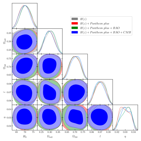
With these considerations, we have plotted one-dimensional and two-dimensional marginalized confidence regions ( and confidence levels) for anisotropic Bumblebee model parameters , , , and for (DS-A), (DS-B), (DS-C) and (DS-D) datasets as shown in Fig. 1.
Table 3 shows the constraints ( and confidence level) on the anisotropic Bumblebee model parameters along with the CDM model parameters from the different available datasets. From Table 3 and Fig. 1, we found that the tightest constraint can be obtained from the DS-D dataset, i.e. joint dataset of on all the cosmological parameters for both the anisotropic Bumblebee model and the CDM model.
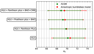
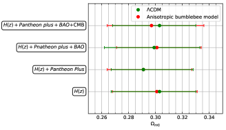
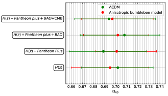
With the use of Table 3, we have tried to compare the , , and parameters for both the models for different dataset combinations within confidence intervals as shown in Fig. 2. The shift of the parameters’ values from the standard CDM model due to anisotropic background and bumblebee field for different combinations of dataset are clearly observed in the plots of these figures. The largest deviations of the cosmological parameters’ from DS-A, DS-B, DS-C and DS-D dataset are compiled in Table 4 for both the standard CDM model and the anisotropic Bumblebee model. From this Table, we can conclude that the deviations are higher in the CDM model in comparison to the anisotropic Bumblebee model.
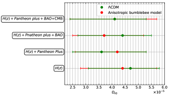
| Model | ||||
|---|---|---|---|---|
| Anisotropic bumblebee | 1.125 | 0.010 | 0.007 | 0.000007 |
| CDM | 1.341 | 0.012 | 0.008 | 0.000011 |
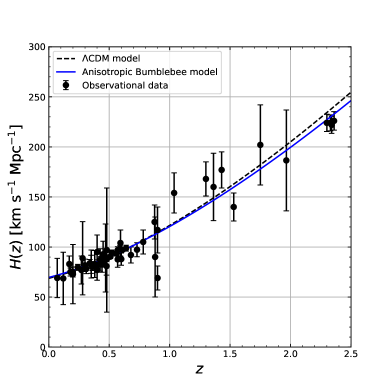
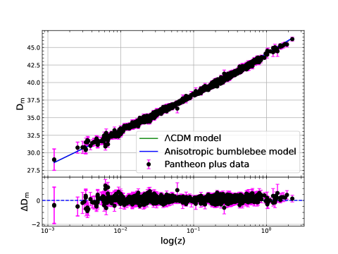
Moreover, we have tried to compare the Hubble parameter versus cosmological redshift variations for both models with the parameters constrained for the DS-D dataset ( dataset) found from the Table 3 as shown in Fig. 3. The plot shows that for the estimated values of cosmological parameters, the Hubble parameter is consistent with the observational data. However, the anisotropic Bumblebee model shows deviations from the standard CDM plot with the increase of cosmological redshift . Thus, from this figure, we have found that the expansion rate of the early Universe for the anisotropic Bumblebee model is slower in comparison to that for the standard CDM model. Similarly, we have plotted the distance modulus () against cosmological redshift in Fig. 4 for the both CDM and anisotropic Bumblebee model along with the distance modulus residue relative to anisotropic Bumblebee model in the logarithmic scale for the constrained set of model parameters as mentioned in the vs plot. The plot shows that like CDM results, the distance modulus for the anisotropic Bumblebee model is consistent with the observational Pantheon plus data obtained from different Type Ia supernovae (SN Ia) for the constrained set of model parameters listed in Table 3. Furthermore, the plot of distance modulus residue also shows that the model is consistent with observational data.
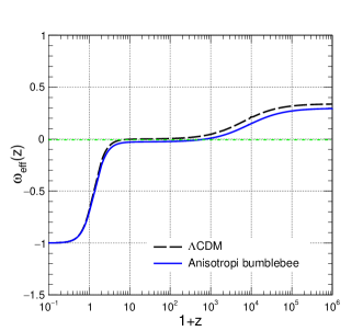

We have plotted the effective equation of state from equation (17) against cosmological redshift for the constrained set of parameters mentioned in Table 3 for both CDM and anisotropic Bumblebee model in the left panel of Fig. 5. The plot shows deviations of the anisotropic Bumblebee model results from the standard CDM results for higher values of , indicating the role of anisotropy and bumblebee field effect in the early stages of the Universe. Apart from the vs plot, we have also plotted the deceleration parameter using equation (18) against the cosmological redshift in the right plot of Fig. 5 for both anisotropic Bumblebee and standard CDM models. In this case also, the anisotropic Bumblebee model results show deviations from the standard CDM results for the higher value of , again indicating the role of anisotropy and the effect of Bumblebee field in the early Universe. However, both plots show that anisotropic Bumblebee cosmology is consistent with the standard cosmology for , i.e. in the present time.
VI Effect of Anisotropy and Bumblebee field on cosmological evolution
In this section, we want to investigate how cosmological evolution can be affected by a considering Bumblebee field in the presence of anisotropy and compare it with the standard CDM results. To this end, we have plotted the density parameters of matter (), radiation () and dark energy () variation with the cosmological redshift for both CDM and anisotropic Bumblebee models indicating the specific features in the plots as shown in Fig. 6.
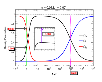
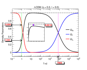
From Fig. 6, we have found that due to the presence of anisotropy and Bumblebee field, the value of for the transition from radiation-dominated to matter-dominated phase in the Universe has been shifted from of standard CDM model to anisotropic Bumblebee model. Thus the anisotropic Bumblebee model suggests an elongated matter-dominated phase. Again, there is a clear sign of an anisotropic effect in terms of obtaining the maximum value of density parameters in the anisotropic Bumblebee model, as its value is much lower than the standard CDM model. In our analysis, we have found that the difference of maximum value from unity for in CDM model is , while in the case of anisotropic bumblebee model, the difference is . Thus, it indicates that there are some effects of anisotropy and bumblebee field on the evolution of the matter-dominated as well as other phases in the Universe. Thus, we can simply say that there are some roles of anisotropy and Bumblebee fields in cosmic evolution.
VII Dynamical system analysis of anisotropic Bumblebee model
In this section, for a dynamical system analysis of anisotropic Bumblebee model we have considered the density parameters , and as dynamical variables and then we have rewritten the equations (14) and (15) as
| (58) | |||
| (59) |
Further, we have renamed the parameter and and derived the derivative for each of them with respect to as
| (60) | ||||
| (61) |
Moreover, the effective equation of state and the deceleration parameter can further be written as
| (62) | ||||
| (63) |
We have compared the critical point analysis for the considered Bumblebee model with the standard CDM results in Table 5.
| Model | Fixed point | Eigenvalues | Remarks | |||||
|---|---|---|---|---|---|---|---|---|
| Anisotropic | (1.058, 4.213) | 0.403 | 1.105 | Unstable point | ||||
| Bumblebee | 0.032 | 0.07 | (-1.058, 3.155) | 0.052 | 0.578 | Saddle point | ||
| (-4.213, -3.154) | -1.0 | -1.0 | Stable point | |||||
| (1, 4) | 0.333 | 1.0 | Unstable point | |||||
| CDM | 0.0 | 0.0 | (-1, 3) | 0.0 | 0.5 | Saddle point | ||
| (-4, -3) | -1.0 | -1.0 | Stable point |

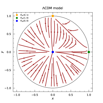
The phase space portrait for the anisotropic Bumblebee model also shows the heteroclinically connected radiation, matter, and dark energy phases as predicted by the standard CDM model (see Fig. 7). However, in contrast to the standard CDM model, the anisotropic Bumblebee model shows that the phases have some anisotropic and Bumblebee field contributions as the critical point solutions and contains no exact unity value. Thus, from this analysis, we can say that both anisotropy and Bumblebee may have some contributions to cosmic evolution.
VIII Conclusions
In this work, we have considered Bumblebee vector model in Bianchi type I Universe and trying to understand its effect on the cosmological parameters and cosmological evolutions of the Universe. Further, we have considered the Universe as a dynamical system and drawn the phase portrait to understand the sequence of different phases of the Universe.
We have started our work by deriving the general form of field equations for the considered model and metric as mentioned above and also obtained the continuity equations in Section IV. In the next section, we have considered the vacuum expectation value (VEV) condition in the field equations of Section III and also obtained the continuity equations for the considered condition. With the help of the field equations, we have further obtained the cosmological parameters like the Hubble parameter (), luminosity distance (), distance modulus (), etc., and carry forward to study these parameters in our next sections.
In Section V, we have constrained our various model parameters that have appeared in the cosmological parameters by using the technique of Bayesian inference. Here, we have used various data compilations for Hubble parameter , Supernovae Type Ia data (Sn Ia), Bao, CMB data, etc. to estimate various model parameters and cosmological parameters which are compiled in Table 3. This table also includes estimated values of cosmological parameters of CDM model. With these sets of parameters, we have compared the values of , , and for both the models within the confidence interval. Moreover, we have plotted the Hubble parameter, and distance modulus along with distance modulus residue with cosmological redshift for the constrained values of model parameters as mentioned above along with the CDM results, and found that the anisotropic Bumblebee model shows good agreement with standard cosmology and consistent with observational data. However, the Hubble parameter shows deviations from the standard CDM results as the value increases. Furthermore, the effective equation of state and deceleration parameters are also plotted against cosmological redshift . Both the plots show good agreement with standard cosmology in the current scenario while, for higher , the anisotropic Bumblebee model shows deviations from the standard results, hence indicating the effect of anisotropy and Bumblebee field in the early Universe.
In Section VI, we have studied the effect of anisotropy and bumblebee field in various density parameters’ evolution. Here, we have compared our results with the standard CDM model and find that there is a shift of the transition point from the radiation-dominated to the matter-dominated phase of the Universe. In our study, we have found that the value of cosmological redshift for the transition from radiation to matter phase is around for CDM model while for the anisotropic bumblebee model, this value shifted to around . Further, we have noticed that the density parameter value never reached unity, hence no pure matter or radiation era, but a mixed state of matter, radiation, and dark energy era. Thus, it is better to say matter-dominated or radiation-dominated state rather than the pure state. Also, we have found that the maximum value of these density parameters is quite lower than standard CDM results. Thus there must be some role of anisotropy and bumblebee field in the cosmic evolution of the Universe.
In Section VII, we have considered the Universe as a dynamical system and hence considered its density parameters as dynamical variables. Subsequently, we studied its stability point analysis for both CDM and anisotropic Bumblebee models. From this anaysis, we have found that the anisotropic Bumblebee model also shows that there are heteroclinically connected radiation-dominated, matter-dominated, and dark energy-dominated phases of the Universe as suggested by standard cosmology, however, there is a shift of critical points from the unity value in anisotropic bumblebee model, which also confirmed the role of anisotropy and Bumblebee field on cosmic evolution as mentioned in Section VI.
Finally, in conclusion, we have observed that with the consideration of anisotropy and the Bumblebee field, the evolution of the Universe i.e. the evolution of the various phases of the Universe is somehow affected and hence may provide an interesting scenario of cosmic expansion. More observational data on the early Universe may help us to understand this scenario more clearly in the near future.
ACKNOWLEDGEMENT
UDG is thankful to the Inter-University Centre for Astronomy and Astrophysics (IUCAA), Pune, India for the Visiting Associateship of the institute.
References
- [1] P. J. E. Peebles, Principles of Physical Cosmology (Princeton University Press)(1994).
- [2] A. G. Riess et al, Observational Evidence from Supernovae for an Accelerating Universe and a Cosmological Constant, Astron. J. 116, 1009 (1998).
- [3] S. Perlmutter et al.,Measurements of and from 42 High-Redshift Supernovae, Asto. Phys. J 517, 565 (1999).
- [4] C. Ma and T.-J. Zhang, Power of observational Hubble parameter data: A figure of merit exploration, Astro. Phys. J. 730 74 (2011)
- [5] V.Trimble, Existence and nature of dark matter in the Universe, Annu. Rev. Astron. Astrophys. 25, 425 (1987).
- [6] J. A. Frieman, M. S. Turner and D. Huterer, Dark Energy and the Accelerating Universe, Annu. Rev. Astron. Astrophys. 46, 385 (2008).
- [7] D. Capelo, J. Pármos, Cosmological implications of bumblebee vector model, Phys. rev. D.91, 104007 (2015).
- [8] V. A. Kostelecky and S. Samuel, Gravitational phenomenology in higher-dimensional theories and strings, Phys. Rev. D 40, 1886 (1989).
- [9] V. A. Kostelecky and S. Samuel, Spontaneous breaking of Lorentz symmetry in string theory, Phys. Rev. D 39, 683 (1989).
- [10] O. Bertolami and J. Páramos, Vacuum solutions of a gravity model with vector-induced spontaneous Lorentz symmetry breaking, Phys. Rev. D 72, 044001 (2005).
- [11] A. De. Felice and S. Tsujikawa, A Cyclic Cosmological Model Based on the Modified Theory of Gravity, Living. rev. Relativity 13, 3 (2010).
- [12] O. Bertolami and J. Páramos, Minimal extension of General Relativity: alternative gravity model with non-minimal coupling between matter and curvature, Int. J. Geom. Methods Mod. Phys. 11, 1460003 (2014).
- [13] I. Zlatev, L. M. Wang and P. J. Steinhardt, Quintessence, cosmic coincidence, and the cosmological constant, Phys. Rev. Lett. 82, 896 (1999).
- [14] A. Tartagila and N. Radicella, Vector field theories in cosmology, Phys. Rev. D. 76, 083501 (2007).
- [15] C. Armendariz-Picon and A. Diez-Tejedor, Aether Unleashed, J. Cosmol. Astropart. Phys. 12, 018 (2019).
- [16] V. A. Kostelecky, Gravity, Lorentz violation, and the standard model, Phys. Rev. D. 69, 105009 (2004).
- [17] R. Bluhm and V. A. Kostelecky, Spontaneous Lorentz violation, Nambu-Goldstone modes, and gravity, Phys. Rev. D. 71, 065008 (2005).
- [18] R. Bluhm, S. H. Fung and V. A. Kostelecky, Spontaneous Lorentz and diffeomorphism violation, massive modes, and gravity, Phys. Rev. D 77, 065020 (2008).
- [19] B. Altschul and V. Kostelecky, Spontaneous Lorentz violation and nonpolynomial interactions, Phys. Lett. B. 628, 106 (2005).
- [20] V. A. Kostelecky and R. Potting, Gravity from spontaneous Lorentz violation,Phys. Rev. D. 79, 065018 (2009).
- [21] V. A. Kostelecky and R. Potting, Gravity from local Lorentz violation, Gen. Relativ. Garvit. 37, 1675 (2005).
- [22] D. J. Gogoi and U. D. Goswami, Quasinormal modes and Hawking radiation sparsity of GUP corrected black holes in bumblebee gravity with topological defects, J. Cosmol. Astropart. Phys. 06, 029 (2022).
- [23] R. Karmakar and U. D. Goswami, Thermodynamics and shadows of GUP-corrected black holes with topological defects in Bumblebee gravity, Phys. Dark. Univ. 41, 101249 (2023).
- [24] N. Aghanim et al., Planck 2018 results. VI. Cosmological parameters, Astron. & Astrophys. 641, A6 (2020).
- [25] A. Chudaykin, D. Gorbunov and N. Nedelko, Exploring an early dark energy solution to the Hubble tension with Planck and SPTPol data, Phys.Rev. D. 103, 043529 (2021).
- [26] H. E. S. Velten, R. F. vom Marttens and W. Zimdahl, Aspects of the cosmological ”coincidence problem”, Eur. Phys. J. C. 74, 3160 (2014).
- [27] G. Hinshaw et al., First-Year Wilkinson Microwave Anisotropy Probe (WMAP) Observations: The Angular Power Spectrum, Astrophys. J. Suppl. 148, 135 (2003).
- [28] G. Hinshaw et al., Three-Year Wilkinson Microwave Anisotropy Probe (WMAP) Observations: Temperature Analysis, Astrophys. J. Suppl. 170, 288 (2007).
- [29] G. Hinshaw et al., Five-Year Wilkinson Microwave Anisotropy Probe Observations: Data Processing, Sky Maps, and Basic Results, Astrophys. J. Suppl. 180, 225 (2009).
- [30] D. J. Eisenstein et. al., Detection of the Baryon Acoustic Peak in the Large-Scale Correlation Function of SDSS Luminous Red Galaxies, Astrophys. J. 633, 560 (2005).
- [31] B. A. Bessett & R. Hlozek, Baryon Acoustic Oscillations, [arXiv:0910.5224] (2009).
- [32] R. B. Tully, C. Howlett and D. Pomarède., Ho’oleilana: An Individual Baryon Acoustic Oscillation?, Astrophys. J. 954, 169 (2023).
- [33] P. A. R. Ade et al., Planck 2015 results XIII. Cosmological parameters, Astron. Astrophys. 594, A13 (2016).
- [34] L. Campanelli, P. Cea, L. Tedesco, Ellipsoidal Universe Can Solve the Cosmic Microwave Background Quadrupole Problem, Phys. Rev. Lett. 97, 131302 (2006).
- [35] Ö. Akarsu, C. B. Kılıç, Bianchi Type-III Models with Anisotropic Dark Energy,Gen. Rel. Grav 42, 109 (2010).
- [36] P. Sarmah, U. D. Goswami, Bianchi Type I model of the universe with customized scale factor, Mod. Phys. Lett. A 37, 21 (2022).
- [37] P.Cea, The Ellipsoidal Universe and the Hubble tension, [arXiv:2201.04548].
- [38] L. Perivolaropoulos, Large Scale Cosmological Anomalies and Inhomogeneous Dark Energy, Galaxies 2(1), 22-61 (2014).
- [39] A. Berera, R.V. Buniy, and T.W. Kephart, The eccentric universe, J. Cosmol. Astropart. Phys. 10, (2004) 016.
- [40] L. Campanelli, P. Cea, L. Tedesco, Ellipsoidal Universe Can Solve the Cosmic Microwave Background Quadrupole Problem, Phys. Rev. Lett. 97, 131302 (2006).
- [41] L. Campanelli, P. Cea, L. Tedesco, Cosmic microwave background quadrupole and ellipsoidal universe, Phys. Rev. D 76, 063007 (2007).
- [42] B. C. Paul and D. Paul, Anisotropic Bianchi-I universe with phantom field and cosmological constant,Pramana J. Phys. 71, 6 (2008).
- [43] J. D. Barrow, Cosmological limits on slightly skew stresses ,Phys Rev. D. 55, 7451 (1997).
- [44] H. Hossienkhani, H. Yousefi and N. Azimi, Anisotropic behavior of dark energy models in fractal cosmology,Int. J. Geom. Methods Mod. Phys. 15 1850200 (2018).
- [45] Ö. Akarsu, S. Kumar, S. Sharma, and L. Tedesco, Constraints on a Bianchi type I spacetime extension of the standard CDM model, Phys. Rev. D 100, 023532 (2019).
- [46] P. Sarmah, A. De and U. D. Goswami, Anisotropic LRS-BI Universe with gravity theory, Phys. Dark. Univ. 40, 101209 (2023).
- [47] P. Sarmah, U. D. Goswami, Dynamical system analysis of LRS-BI Universe with gravity theory, Phys. Dark. Univ. 46, 101556 (2024).
- [48] F. Esposito et al.,Reconstructing isotropic and anisotropic cosmologies, Phys. Rev. D 105, 084061 (2022).
- [49] Z. F. Mai et al., Extended thermodynamics of the bumblebee black holes, Phys. Rev. D. 108, 024004 (2023).
- [50] J. Gu et al., Probing bumblebee gravity with black hole X-ray data, Eur. Phys. J. C, 82, 708 (2022).
- [51] Í. Sakalli, and E. Yörük, Modified Hawking radiation of Schwarzschild-like black hole in bumblebee gravity model, Phys. Scr., 98, 125307 (2023).
- [52] R. V. Maluf and J. C. S. Neves, Bumblebee field as a source of cosmological anisotropies, J. Cosmol. Astropart. Phys.10, 038,(2021).
- [53] J. C. S. Neves, Kasner cosmology in bumblebee gravity, Annal. Phys. 454, 169338 (2023).
- [54] C. Zhang et al., Four New Observational Data From Luminous Red Galaxies of Sloan Digital Sky Survey Data Release Seven, Res. Astron. Astrophys 14, 1221 (2014).
- [55] J. Simon et al., Constraints on the redshift dependence of the dark energy potential, Phys. Rev. D 71, 123001 (2005).
- [56] M. Moresco et al., Improved constraints on the expansion rate of the Universe up to from the spectroscopic evolution of cosmic chronometers, JCAP 08, 006 (2012).
- [57] E. Gaztan̄aga et al., Clustering of luminous red galaxies-IV. Baryon acoustic peak in the line-of-sight direction and a direct measurement of ,MNRAS 399, 1663 (2009).
- [58] A. Oka et al., Simultaneous constraints on the growth of structure and cosmic expansion from the multipole power spectra of the SDSS DR7 LRG sample, Mon. Not. Roy. Astron. Soc. 439, 2515 (2014).
- [59] Y. Wang et al.,The clustering of galaxies in the completed SDSS-III Baryon Oscillation Spectroscopic Survey: tomographic BAO analysis of DR12 combined sample in configuration space, Mon. Not. Roy. Astron. Soc. 469, 3762 (2017).
- [60] X. Xu et al., Measuring and at from the SDSS DR7 LRGs using baryon acoustic oscillation, Mon. Not. Roy. Astron. Soc. 431, 2834 (2013).
- [61] S. Alam et al., The clustering of galaxies in the completed SDSS-III Baryon Oscillation Spectroscopic Survey: cosmological analysis of the DR12 galaxy sample, Mon. Not. Roy. Astron. Soc. 470, 2617 (2017).
- [62] M. Moresco et al., A measurement of the Hubble parameter at : direct evidence of the epoch of cosmic re-acceleration, JCAP 05, 014 (2016).
- [63] C. Blake et al., The WiggleZ dark energy survey: Joint measurements of the expansion and growth history at , Mon. Not. Roy. Astron. Soc. 425, 405 (2012).
- [64] A. L. Ratsimbazafy et al., Age-dating luminous red galaxies observed with the Southern African Large Telescope,Mo. Not. Roy. Astron. Soc. 467, 3239 (2017).
- [65] L. Samushia et al., The clustering of galaxies in the SDSS-III DR9 Baryon Oscillation Spectroscopic Survey: testing deviations from and general relativity using anisotropic clustering of galaxies, Mon. Not. Roy. Astron. Soc. 429, 1514 (2013).
- [66] C. H. Chuang et al., The clustering of galaxies in the SDSS-III Baryon Oscillation Spectroscopic Survey: single-probe measurements and the strong power of on constraining dark energy ,Mon. Not. Roy. Astron. Soc. 433, 3559 (2013).
- [67] M. Moresco, Raising the bar: new constraints on the Hubble parameter with cosmic chronometers at , Mon. Not. Roy. Astron. Soc. 450, L16 (2015).
- [68] N. G. Busca et al., Baryon acoustic oscillations in the forest of BOSS quasars, Astron. Astrophys. 552, A96 (2013).
- [69] J. E. Bautista et al., Measurement of baryon acoustic oscillation correlations at with SDSS DR12 - Forests, Astron. Astrophys. 603, A12 (2017).
- [70] T. Delubac et al., Baryon acoustic oscillations in the forest of BOSS DR11 quasars,Astron. Astrophys. 574, A59 (2015).
- [71] A. F. Ribera et al., Quasar-Lyman forest cross-correlation from BOSS DR11: Baryon Acoustic Oscillations, J. Cosmol. Astropart. Phys. 05, 027 (2014).
- [72] J. R. Cooke et al., The primordial deuterium abundance of the most metalpoor damped Ly system, Astrophys. J., 496, 605 (1998).
- [73] S. Dodelson, Modern Cosmology (Academic Press, New York) (2003).
- [74] F. Beutler et al., The 6dF galaxy survey: Baryon acoustic oscillation and the local Hubble constant, Mon. Not. R. Astron. Soc. 416, 3017 (2011).
- [75] A. J. Ross et al, The clustering of the SDSS DR7 main Galaxy sample- I. A 4 percent distance measure at z = 0.15, Mon. Not. R. Astron. Soc. 449, 835 (2015).
- [76] N. Padmanabhan et al., A 2 distance to z = 0.35 by reconstructing baryon acoustic oscillations I. Methods and application to the Solan digital sky survey, Mon. Not. R. Astron. Soc. 427, 2132 (2012).
- [77] L. Anderson et al., The clustering of galaxies in the SDSS-III Baryon oscillation spectroscopic survey: Baryon acoustic oscillations in the data release 10 and 11 Galaxy samples, Mon. Not. R. Astron. Soc. 441, 24 (2014).
- [78] M. Betoule et. al, Improved cosmological constraints from a joint analysis of the SDSS-II and SNLS supernova samples, Astron. Astrophys. 568, A22 (2014).
- [79] D. Scolnic et al., The Pantheon Analysis: The Full Data Set and Light-curve Release, Astropys. J., 938, 113 (2022).
- [80] D. Zhao, Y. Zhou, and Z. Chang, Anisotropy of the Universe via the Pantheon supernovae sample revisited, 486, 5679 (2019).
- [81] D. Scolnic et al., The complete light-curve sample of spectroscopically confirmed SNe Ia from Pan-STARRS1 and cosmological constraints from the combined Pantheon sample, Astrophys. J. 859, 101 (2018).
- [82] J. Páramos and G. Guiomar, Astrophyisical Constraints on the Bumblebee model, Phys. Rev. D 90, 082002 (2014).