SUPPLEMENTAL MATERIAL
Measuring dynamical phase transitions in time series

Abstract

There is a growing interest in methods for detecting and interpreting changes in experimental time evolution data. Based on measured time series, the quantitative characterization of dynamical phase transitions at bifurcation points of the underlying chaotic systems is a notoriously difficult task. Building on prior theoretical studies that focus on the discontinuities at $q=1$ in the order-$q$ Rényi-entropy of the trajectory space, we measure the derivative of the spectrum. We derive within the general context of Markov processes a computationally efficient closed-form expression for this measure. We investigate its properties through well-known dynamical systems exploring its scope and limitations. The proposed mathematical instrument can serve as a predictor of dynamical phase transitions in time series.

.1 Entropies

Here we summarize the entropy-related definitions from the main paper. The order-$q$ Rényi entropy for a discrete distribution $\bm{p}=(p_{1},p_{2},\dots,p_{N})$ is defined as

$$H_{q}(\bm{p})=\frac{1}{1-q}\ln\sum_{i=1}^{N}p_{i}^{q}\,,$$ (1)

where $H_{q}\geq H_{q^{\prime}}$ whenever $q^{\prime}>q$ . The Shannon entropy of the same distribution can be obtained in the $q=1$ limit, as the mean

$$H_{1}(\bm{p})=-\langle\ln\bm{p}\rangle_{\bm{p}}=-\sum_{i=1}^{N}p_{i}\ln p_{i}\,.$$ (2)

The same limit of the derivative of the Rényi-entropy, with respect to $q$, gives the variance

$$H_{1}^{\prime}(\bm{p})=-\frac{1}{2}\Delta^{2}_{\bm{p}}\ln(\bm{p})=-\frac{1}{2}\left(\langle\ln^{2}\bm{p}\rangle_{\bm{p}}-\langle\ln\bm{p}\rangle^{2}_{\bm{p}}\right)\,.$$ (3)

For a dynamical system with coarse-grained natural distribution ${\bm{\rho}}^{*}$ on the attractor we denote with

$$C_{1}=H_{1}({\bm{\rho}}^{*})\,,\qquad C_{2}=-2H^{\prime}_{1}({\bm{\rho}}^{*})\,.$$ (4)

The dynamical Rényi-entropy is defined as the time-normalized entropy of the trajectory probabilities ${\mathbfcal{P}}$:

$$K_{q}({\mathbfcal{P}})=\lim_{t\rightarrow\infty}\frac{1}{t}H_{q}({\mathbfcal{P}}(t))\,.$$ (5)

The $q=1$ value is of special interest, and it is called the Kolmogorov-Sinai entropy or metric entropy [1]:

$$S=K_{1}({\mathbfcal{P}})\,,\qquad\Lambda=-{2}K_{1}^{\prime}({\mathbfcal{P}})\,.$$ (6)

.2 Markov chain formalism

Left and right eigenvectors, ${\bm{\rho}}_{\nu}^{\top}$ and $\mathbf{v}_{\nu}$, respectively, of the stochastic matrix $\mathbf{W}=(w_{ij})$, with $i,j=1,\dots,N$, are defined as:

$$\mathbf{W}^{\top}{\bm{\rho}}_{\nu}=\alpha_{\nu}\cdot{\bm{\rho}}_{\nu}\,,\qquad\qquad\mathbf{W}\mathbf{v}_{\nu}=\alpha_{\nu}\cdot\mathbf{v}_{\nu}\,,$$ (7)

with $\alpha_{\nu}$ eigenvalues, where $\alpha_{1}=1$, and ${\bm{\rho}}_{1}$ is the stationary distribution of the corresponding Markov chain, for which the normalization is given by ${\bm{\rho}}_{1}^{\top}\mathbf{v}_{1}=1$ with $\mathbf{v}_{1}=(1,1,\dots,1)$. Note that as symbols with zero probability play no role in this representation, the stationary distribution of the Markov chain ${\bm{\rho}}_{1}$, for states of order $m=1$, provides an approximation of the natural distribution on the attractor ${\bm{\rho}}^{*}$ when omitting cells with zero probability, ${\bm{\rho}}_{1}={\bm{\rho}}^{*}$.

A useful identity concerning the powers of the transition matrix is

$$\left(\mathbf{W}-\alpha_{\nu}\mathbf{v}_{\nu}{\bm{\rho}}_{\nu}^{\top}\right)^{k}=\mathbf{W}^{k}-\alpha_{\nu}^{k}\mathbf{v}_{\nu}{\bm{\rho}}_{\nu}^{\top}\,,\qquad\quad k\geq 1\,.$$ (8)

In the following we denote ${\bm{\rho}}={\bm{\rho}}_{1}$ and $\mathbf{1}=\mathbf{v}_{1}$ for simplicity.

.3 Rényi entropy spectrum

The full spectrum of the truncated Rényi-entropies can be given as

$$\tilde{K}_{q}=\frac{1}{1-q}\lim_{k\rightarrow\infty}\frac{1}{k}\ln\left(\sum_{i,j}\rho_{i}^{q}(\mathbf{W}_{q}^{k})_{ij}1_{j}\right)=$$

$$\frac{1}{1-q}\lim_{n\rightarrow\infty}\ln\left(\frac{\sum_{i,j}\rho_{i}^{q}(\mathbf{W}_{q}^{k+1})_{ij}1_{j}}{\sum_{i,j}\rho_{i}^{q}(\mathbf{W}_{q}^{k})_{ij}1_{j}}\right)=$$

$$\frac{\ln\alpha_{\text{max}}(q)}{1-q}\,,$$ (9)

where $\alpha_{\text{max}}(q)$ is the largest eigenvalue of the $(\mathbf{W}_{q})_{ij}=w_{ij}^{q}$ matrix (element-wise $q$ power). According to the Perron-Frobenius theorem for irreducible non-negative matrices the spectral radius $\alpha_{\text{max}}$ is a positive real number.

For random systems (without memory), viz. for $w_{ij}=1_{i}\rho_{j}$, where $1_{i}$ denotes the $i$-th component of a vector of all-ones, the above expression reduces to the Rényi entropy of the stationary distribution,

$$\tilde{K}_{q}=\frac{1}{1-q}\ln\sum_{i=1}^{N}\rho_{i}^{q}=H_{q}({\bm{\rho}})\,.$$ (10)

Hence, for memory-less dynamics and first-order states, the truncated estimation of the entropy rate, $S$, and diffusion coefficient, $\Lambda$, from Eq. (6) turn into the bit-number statistics, $C_{1}$ and $C_{2}$, from Eq. (4).

.4 Path length statistics and entropies

Using the notations ${\mathbfcal{P}}(t)\equiv\rho_{s_{1}}{\mathbfcal{P}}(\mathbfcal{X}(t)|s_{1})$ for the set of probabilities of all trajectories of $t$ steps, and $\mathbfcal{L}(t)\equiv-\ln{\mathbfcal{P}}(\mathbfcal{X}(t)|s_{1})$ for the length of trajectories with given initial state, Eqs. (1) and (5) can be combined into

$${K}_{1}({\mathbfcal{P}}) =-\lim_{t\rightarrow\infty}\frac{1}{t}\langle\ln{\mathbfcal{P}}(t)\rangle_{\mathbfcal{P}}=$$

$$=-\lim_{t\rightarrow\infty}\frac{1}{t}\left({\langle\ln{\bm{\rho}}\rangle_{{\bm{\rho}}}}-\langle\mathbfcal{L}(t)\rangle_{\mathbfcal{P}}\right)=$$

$$=\lim_{t\rightarrow\infty}\frac{1}{t}\langle\mathbfcal{L}(t)\rangle_{\mathbfcal{P}}\,,$$ (11)

where averaging is done over all states $s_{i}$, realizations of trajectories $\mathcal{X}(t)$ of length $t$ and initial states $s_{1}$, respectively.

Similarly, Eqs. (3) and (5) yield

$${K}_{1}^{\prime}({\mathbfcal{P}})=-\lim_{t\rightarrow\infty}\frac{1}{2t}\Delta_{\mathbfcal{P}}^{2}\ln({\mathbfcal{P}}(t))\,.$$ (12)

Since generally $\Delta^{2}(x+y)=\Delta^{2}x+\Delta^{2}y+2\text{Cov}(x,y)$ for random variables $x$ and $y$, and the covariance between $\rho_{i}$ and $\mathcal{P}(\mathcal{X}(t)|s_{1})$ goes to zero as the number of steps, $t$, goes to infinity, $\mathrm{Cov}(\rho_{i},\mathcal{P}(\mathcal{X}(t)|s_{1}))\rightarrow 0$, we get

$${K}_{1}^{\prime}({\mathbfcal{P}}) =-\lim_{t\rightarrow\infty}\frac{1}{2t}\left(\Delta_{\bm{\rho}}^{2}\ln{\bm{\rho}}+\Delta_{\mathbfcal{P}}^{2}\mathbfcal{L}(t)\right)=$$

$$=-\lim_{t\rightarrow\infty}\frac{1}{2t}\Delta_{\mathbfcal{P}}^{2}\mathbfcal{L}(t)\,.$$ (13)

.5 Interpretation of the KS entropy

The entropy rate determines the mean of the normal distribution, see Eq. (11), and can be interpreted as the amount of uncertainty removed by evolving the Markov chain with one step:

$$S=\sum_{i}^{N}\rho_{i}S_{i}\,,\qquad S_{i}=-\sum_{j}^{N}w_{ij}\ln w_{ij}\,,$$ (14)

averaged over all state entropies $S_{i}$. The KS entropy can be decomposed into the difference between the transition’s entropy and the entropy of the stationary distribution of states:

$$S=S_{\mathrm{tr}}-C_{1}$$ (15)

where

$$S_{\mathrm{tr}}=-\sum_{i,j}^{N}\rho_{i}w_{ij}\ln\left(\rho_{i}w_{ij}\right)\,,\quad C_{1}=-\sum_{i}^{N}\rho_{i}\ln\rho_{i}$$ (16)

are respectively the transition entropy and state entropy, compare Eq. (4). Note that using transition probabilities and $q=1$ we get a proper extensive (in time) statistical physics. The mean bit number $C_{1}$ has, however, no straightforward interpretation as an extensive quantity.

.6 Lyapunov measure as ensemble averages

In order to compute the Lyapunov measure $\Lambda$, first we need to estimate the auto-covariances,

$$\mathrm{Cov}(l_{1},l_{1+\tau})=\langle l_{1}l_{1+\tau}\rangle-\langle l_{1}\rangle\langle l_{1+\tau}\rangle\,,$$ (17)

for all possible time-lags $\tau$, where $l_{1}$ is the edge length in the first step. Due to the stationarity of the process, considering an ensemble of random walkers with initial distribution ${\bm{\rho}}$, the ensemble-averaged step length is constant along the $\tau=1,\dots,t$ steps of the random walks, $\langle l\rangle=\langle l_{\tau}\rangle$, and it can be expressed as:

$$\langle l\rangle=-\sum_{i=1}^{N}\rho_{i}\sum_{j=1}^{N}w_{ij}\ln w_{ij}={\bm{\rho}}^{\top}\mathbf{L}_{1}\mathbf{1}\,,$$ (18)

where $(\mathbf{L}_{1})_{ij}=-w_{ij}\ln w_{ij}$ is the probability-weighted edge-length matrix. Note also that for $t\gg 1$ the ensemble-averaged edge lengths during the random walks do not depend on the starting positions of the walks.

Now, considering time-lags $\tau\in\{1,2,\dots\}$ we calculate the $\tau$-th order covariance of step-lengths $l$,

$$\langle l_{1}l_{{1+\tau}}\rangle=$$

$$= \sum\limits_{s_{1}=1}^{N}\rho_{s_{1}}\sum\limits_{s_{2}=1}^{N}w_{s_{1}s_{2}}(-\ln w_{s_{1}s_{2}})\sum\limits_{s_{3}=1}^{N}w_{s_{2}s_{3}}\dots$$

$$...\sum\limits_{s_{\tau+1}=1}^{N}w_{s_{\tau}s_{\tau+1}}(-\ln w_{s_{\tau}s_{\tau+1}})=$$

$$={\bm{\rho}}^{\top}\mathbf{L}_{1}\mathbf{W}^{\tau-1}\mathbf{L}_{1}\mathbf{1}\,.$$

Using identity (8) with $\alpha_{1}=1$, for the infinite sum of covariances we need to calculate

$$\mathbf{B}=\sum_{\tau=1}^{\infty}(\mathbf{W}^{\tau-1}-\mathbf{W}^{\infty})=\sum_{k=0}^{\infty}(\mathbf{W}^{k}-\mathbf{1}{\bm{\rho}}^{\top})=$$

$$=(\mathbf{I}-\mathbf{1}{\bm{\rho}}^{\top})+\sum_{k=1}^{\infty}(\mathbf{W}-\mathbf{1}{\bm{\rho}}^{\top})^{k}\,,$$

where $\mathbf{W}^{\infty}\equiv\lim_{k\rightarrow\infty}\mathbf{W}^{k}$. Denoting with $\mathbf{A}=\mathbf{W}-\mathbf{1}{\bm{\rho}}^{\top}$ and knowing that $\mathbf{W}^{\infty}=\mathbf{1}{\bm{\rho}}^{\top}$ the sum

$$\lim_{k\rightarrow\infty}\sum_{i=1}^{k}\mathbf{A}^{i}=\lim_{k\rightarrow\infty}\mathbf{A}(\mathbf{I}-\mathbf{A})^{-1}(\mathbf{I}-\mathbf{A}^{k+1})=\mathbf{A}(\mathbf{I}-\mathbf{A})^{-1}\,,$$ (19)

since from Eq. (8) $\lim_{k\rightarrow\infty}\mathbf{A}^{k}=\mathbf{0}$.

Finally, we have

$$\mathbf{B}=(\mathbf{I}-\mathbf{1}{\bm{\rho}}^{\top})+(\mathbf{W}-\mathbf{1}{\bm{\rho}}^{\top})(\mathbf{I}-\mathbf{W}+\mathbf{1}{\bm{\rho}}^{\top})^{-1}\,,$$ (20)

and hence the infinite sum of auto-covariances from Eq. (17) is given by

$$\sum_{\tau=1}^{\infty}\mathrm{Cov}(l_{1},l_{1+\tau}) =\sum_{\tau=1}^{\infty}{\bm{\rho}}^{\top}\mathbf{L}_{1}\,(\mathbf{W}^{\tau-1}-\mathbf{W}^{\infty})\mathbf{L}_{1}\,\mathbf{1}=$$

$$={\bm{\rho}}^{\top}\,\mathbf{L}_{1}\,\mathbf{B}\,\mathbf{L}_{1}\,\mathbf{1}\,.$$ (21)

Bringing everything together, the variance of individual edge lengths is

$$\sigma_{l}^{2}=\langle l^{2}\rangle-\langle l\rangle^{2}\ ={\bm{\rho}}^{\top}\mathbf{L}_{2}\,\mathbf{1}-({\bm{\rho}}^{\top}\mathbf{L}_{1}\,\mathbf{1})^{2}\,,$$ (22)

where $(\mathbf{L}_{2})_{ij}=w_{ij}\ln^{2}w_{ij}$, the entropy rate can be expressed by using Eq. (18) as

$$S={\bm{\rho}}^{\top}\mathbf{L}_{1}\mathbf{1}\,,$$ (23)

while the Lyapunov measure is given by the

$$\Lambda={\bm{\rho}}^{\top}\mathbf{L}_{2}\,\mathbf{1}-({\bm{\rho}}^{\top}\mathbf{L}_{1}\,\mathbf{1})^{2}+2{\bm{\rho}}^{\top}\mathbf{L}_{1}\,\mathbf{B}\,\mathbf{L}_{1}\,\mathbf{1}$$ (24)

closed-form expression, where ${\bm{\rho}}^{\top}$ and $\mathbf{1}=(1,1,\dots,1)$ are the left and right eigenvectors of the stochastic transition matrix $\mathbf{W}$ with eigenvalue $\alpha_{1}=1$, and

$$\mathbf{B}\equiv(\mathbf{I}-\mathbf{W}+\mathbf{1}{\bm{\rho}}^{\top})^{-1}-\mathbf{1}{\bm{\rho}}^{\top}\,.$$ (25)

For systems defined by a random transition matrix $\mathbf{W}$ with uniformly distributed elements, the Lyapunov-measure $\Lambda$ approaches 1/4 as the number of states goes to infinity [2].

.7 Numerical results for prototypical examples

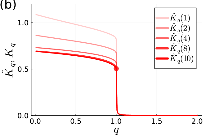
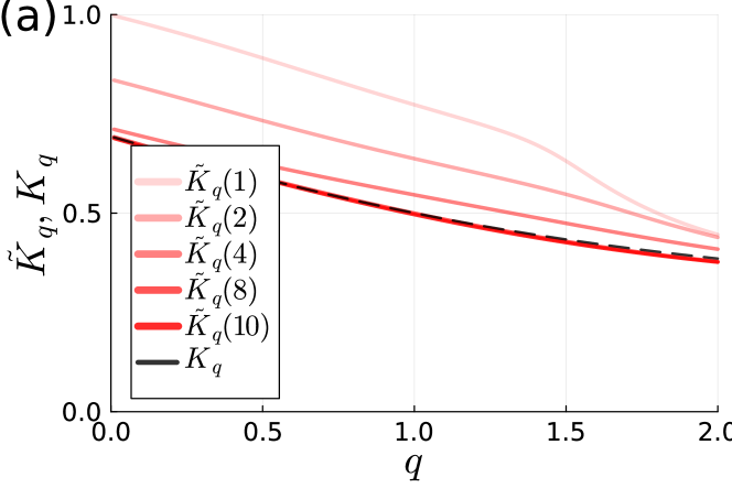
Figure 1: Spectrum of the truncated Rényi entropy $\tilde{K}_{q}(m)$ of two different maps computed by using Eq. (9) and states of order $m$ for trajectories of $10^{8}$ steps on the attractor, after discarding the first $10^{6}$ steps. (a) The asymmetric tent map defined by Eq. (26) with parameter $r=0.8$ using uniform partitioning to $n=2^{5}$ cells. The corresponding analytical entropy values, $K_{q}$, of Eq. (27) are shown by the dashed line. (b) The critical map from Eq. (28) with parameter $r=2$ using uniform partitioning to $n=2^{10}$ cells. The red marker denotes the $\tilde{K}_{1}(10)\approx K_{1}=0.5$ value [3]. For (a) and (b), the [0,1] interval has been partitioned into the given number of cells $n$.

In addition to the examples in the main paper we consider the asymmetric tent map [4]:

$$x_{\tau+1}=\begin{cases}\dfrac{x_{\tau}}{r}\ ,&\quad\text{for }0\leq x<r\,,\\ \\ \dfrac{1-x_{\tau}}{1-r}\ ,&\quad\text{for }r\leq x\leq 1\,,\end{cases}$$ (26)

where $r\in(0,1)$ and for which the $[0,r)$ and $[r,1)$ cells are generating and Markov partitions at the same time [4]. For this system, the analytical expression for the Rényi entropy is [4]:

$$K_{q}=\ln(r^{q}+(1-r)^{q})/(1-q)\ .$$ (27)

Estimating the transition probability matrix $\mathbf{W}$ from a sufficiently long trajectory of the system from Eq. (26) and using the Markov partitions from above, the entropies from Eqs. (27) and (9) coincide, $\tilde{K}_{q}=K_{q}$ (not shown here). For a partitioning composed of e.g. $n=2^{5}$ equally-sized cells combined with higher-order states, the truncated entropy in Eq. (9) together with order $m=10$ provides a reasonably good estimate of the exact Rényi entropy spectrum given by Eq. (27), as shown in panel (a) of Fig. 1.

Another example is the family of critical systems [3]:

$$x_{\tau+1}=1-\left|x_{\tau}^{r}-(1-x_{\tau})^{r}\right|^{1/r}\,,$$ (28)

exhibiting intermittent dynamics. These systems present a dynamical phase transition at $q=1$ [3]. Constructing the Markov chain representation of the dynamics using $n=2^{10}$ equal-sized bins, and higher-order states with $m=10$, the Rényi entropy spectrum is computed using Eq. (9) and shown in Fig. 1(a). Though the absolute value of the truncated entropy $\tilde{K}_{q}$ depends on the resolution $n$ and the order $m$, the qualitative nature of the phase transition is unaffected (see Fig. 1(b)). The exact value of the KS/metric entropy $S=0.5$ [3] is approximated well already for $m=10$ by $\tilde{K}_{1}$.

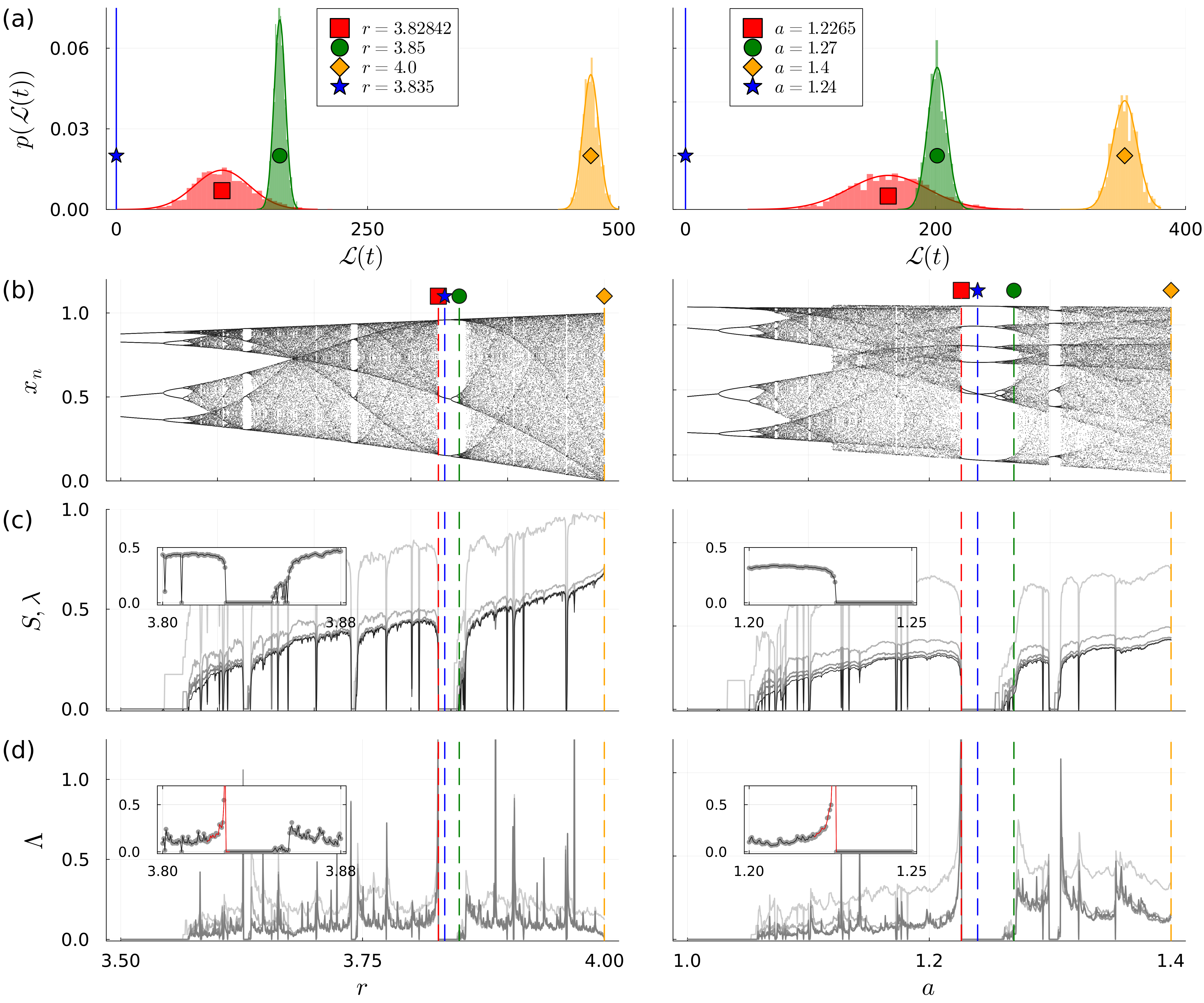
Figure 2: Matching the classical picture of the logistic map (left column) and the Henon map (right column) to its Markov-chain-based model. The first $10^{6}$ time steps preceding the $10^{8}$ total number of steps were discarded in order to eliminate the transients. For the logistic map, the [0,1] interval is partitioned into $n=2^{5}$ equally sized cells and iterated for 1000 different values of the control parameter $r$ covering the [3.5, 4] range. Similarly, for the Henon map the phase plane $[-2,2]\times[-2,2]$ is partitioned into a $n=2^{5}\times 2^{5}$ grid and iterated for 1000 different values of the control parameter $a$ covering the [1.0, 1.4] range. The parameter values $r$ and $a$ used as examples in panels (a) and (b) of Fig. 1 of the main paper, respectively, are indicated by the corresponding markers and the vertical dashed lines. (a) Demonstration of the effect of the central-limit theorem for Markov chains on the total path lengths, $\mathcal{L}(t)$, in the limit $t\rightarrow\infty$. Histograms are obtained from 10³ random walk simulations of length $t=500$ on the corresponding $m=1$ (first-order) state-transition networks (STN). Continuous lines represent the normal distributions with mean $\langle\mathcal{L}(t)\rangle=S(m=1)\cdot t$ and variance $\Delta^{2}\mathcal{L}(t)=\Lambda(m=1)\cdot t$, where the KS entropy $S$ and Lyapunov measure $\Lambda$ are computed based on Eqs. (23) and (24). (b) The bifurcation (orbit) diagrams of the two systems. (c) The KS entropy, $S(m)$, and (d) the Lyapunov measure, $\Lambda(m)$. Lines in increasingly darker shades of gray correspond to Markov chains using states of order $m=1,2,4,12$, respectively. In panel (c) the largest Lyapunov exponent, $\lambda$, is also shown by the thin black line for comparison. Note that $S(12)\approx\lambda$ for $\lambda>0$. The analytical results (gray lines) given in Eq. (24) are compared to the statistics of 1000 simulated random walks of 500 steps (gray circular markers) on the corresponding STNs in the insets for order $m=12$ with the divergent $\Lambda$ values preceding the bifurcations marked by the red curves.

Fig. 2 provides further details on the logistic and Henon maps compared to Fig. 1 in the main paper. Panel (a) demonstrates numerically the effect of central-limit theorem for Markov chains on the total path lengths, $\mathcal{L}(t)$, in the limit of $t\rightarrow\infty$.

.8 Numerical estimation of $S$ and $\Lambda$

The computational complexity of evaluating $S$ in Eq. (23) and the first two terms of $\Lambda$ in Eq. (24) are of $\mathcal{O}(N^{2})$ where $N$ is the number of symbols. The third term contains a matrix inverse but in conjunction with the inner product allowing for the application of a linear solver instead of inversion. More precisely we are looking for the vector

$$\mathbf{z}=(\mathbf{I}-\mathbf{W}+\mathbf{1}{\bm{\rho}}^{\top})^{-1}\mathbf{L}_{1}\mathbf{1}\;.$$

Since the number of symbols increases exponentially with the order of the representation the computational cost of the inverse calculation becomes prohibitive for high orders. However, in this case, $\mathbf{W}$ becomes a sparse matrix facilitating the use of high-efficiency iterative solvers. The solution in $\mathbf{z}$ is obtained as the fix-point of the iteration

$$\mathbf{z}^{\prime}=\mathbf{W}\mathbf{z}-\mathbf{1}\langle z\rangle+\mathbf{L}_{1}\mathbf{1}\;.$$

where $\langle z\rangle\equiv{\bm{\rho}}^{\top}\mathbf{z}$. Using a random vector as an initial value of $\mathbf{z}$ the iteration is convergent for all systems studied here.

.9 CODE AVAILABILITY

The full code base has been released on Github, see Ref. [5]. The basic functionalities as computing the symbolic representation, the transition matrix, and the corresponding measures are implemented in our Julia package, StateTransitionNetworks.jl. Main results included in this work can be repeated from scratch with the codes in the ’stn_paper’ directory (see the attached README file).