Correcting the Mythos of KL-Regularization:
Direct Alignment without Overoptimization via $\chi^{2}$-Preference Optimization

Abstract

Language model alignment methods, such as reinforcement learning from human feedback (RLHF), have led to impressive advances in language model capabilities, but existing techniques are limited by a widely observed phenomenon known as overoptimization, where the quality of the language model plateaus or degrades over the course of the alignment process. Overoptimization is often attributed to overfitting to an inaccurate reward model, and while it can be mitigated through online data collection, this is infeasible in many settings. This raises a fundamental question: Do existing offline alignment algorithms make the most of the data they have, or can their sample-efficiency be improved further?

We address this question with a new algorithm for offline alignment, $\chi^{2}$-Preference Optimization ($\chi$PO).

$\chi$PO is a one-line change to Direct Preference Optimization (DPO; Rafailov et al. (2023)), which only involves modifying the logarithmic link function in the DPO objective. Despite this minimal change, $\chi$PO implicitly implements the principle of pessimism in the face of uncertainty via regularization with the $\chi^{2}$-divergence—which quantifies uncertainty more effectively than KL-regularization—and provably alleviates overoptimization, achieving sample-complexity guarantees based on single-policy concentrability—the gold standard in offline reinforcement learning. $\chi$PO’s simplicity and strong guarantees make it the first practical and general-purpose offline alignment algorithm that is provably robust to overoptimization.

1 Introduction

Large language models (LLMs) trained on unsupervised text data exhibit impressive and surprising capabilities (Brown et al., 2020; Ouyang et al., 2022; Touvron et al., 2023; OpenAI, 2023; Google, 2023), but can be difficult to control without further guidance. Reinforcement learning from human feedback (RLHF) and other alignment methods have emerged as a central tool to align these models to human values and elicit desired behavior (Christiano et al., 2017; Bai et al., 2022; Ouyang et al., 2022; Rafailov et al., 2023). This is achieved by treating the language model as a policy, and using techniques from reinforcement learning to optimize for desirable outcomes under a (explicit or implicit) reward model learned from a dataset of human-labeled responses.

Alignment methods like RLHF have led to significant advances in language model capabilities, particularly in chat domains, but existing techniques are limited by a widely observed phenomenon known as reward overoptimization or reward hacking (Michaud et al., 2020; Tien et al., 2022; Gao et al., 2023; Rafailov et al., 2024a). Since the reward model used implicitly or explicitly by these methods is an imperfect proxy for human preferences, the true quality of the language model can degrade as training proceeds, even as performance under the reward model continues to improve. Intuitively, this occurs because the language model may drift away from the manifold covered by the human-labeled data used to train the reward model and end up in a region where the reward model is inaccurate.

Overoptimization is distinct from the classical concept of overfitting because it is a causal or counterfactual phenomenon: When the human-labeled dataset does not cover all possible alternatives, the decision maker—in this case, a language model policy—cannot directly evaluate the effect of their actions. This perspective is supported by the fact that overoptimization can be mitigated by online alignment techniques (Guo et al., 2024; Gao et al., 2024; Dong et al., 2024), which exploit interactive access to human or AI feedback to iteratively improve the reward model; unfortunately, gathering such feedback is costly and impractical in many settings. This raises natural questions regarding the role of overoptimization in offline alignment:

• Is overoptimization in offline alignment an information-theoretic phenomenon? This would mean that there is simply not enough information in the human-labeled (offline) preference dataset due to partial coverage, and no algorithmic intervention (e.g., early stopping), no matter how clever, can avoid the overoptimization issue.

• Alternatively, is overoptimization an algorithmic phenomenon? This would mean that existing algorithms are not making the most of the data they have (e.g., due to optimizing the wrong objective and converging toward suboptimal solutions) and would suggest that their sample-efficiency can be improved, perhaps by taking more aggressive measures to avoid overfitting to the reward model.

Parallel developments in the theory of offline reinforcement learning suggest that the answer may be the latter. Indeed, this literature has addressed the challenge of overoptimization—typically referred to as distribution shift—through the principle of pessimism in the face of uncertainty. The principle of pessimism asserts that given an offline dataset with partial coverage, a decision maker should choose their response according to the most pessimistic view of the world supported by the data. Pessimism encourages the model to avoid overfitting to the offline dataset and is supported by a rich theory, showing that it offers provable robustness to overoptimization in stylized settings (Liu et al., 2020; Jin et al., 2021; Rashidinejad et al., 2021).

Perhaps the greatest barrier to implementing pessimism for language models is to efficiently quantify uncertainty in the learned reward model and distill this understanding into an actionable form. This is particularly challenging due to the combinatorial nature of the space of responses. A natural approach that forms the basis of most existing offline alignment methods (Christiano et al., 2017; Bai et al., 2022; Ouyang et al., 2022; Rafailov et al., 2023) is to use KL-regularization to encourage the learned policy to stay close to a reference policy (typically obtained through supervised fine-tuning and used to collect the offline data), but this form of regularization is insufficient to induce pessimism (Gao et al., 2023), and is provably suboptimal in theory (Zhu et al., 2023; Song et al., 2024, see also Section A.1). On the other hand, offline reinforcement learning theory offers abstract pessimistic algorithms that are suitable—at least statistically—for large models (Xie et al., 2021; Uehara and Sun, 2021; Zhan et al., 2022; Chen and Jiang, 2022), but cannot be implemented directly without losing fidelity to the theory or making unrealistic modeling assumptions (Zhu et al., 2023; Zhan et al., 2023b; Li et al., 2023; Xiong et al., 2023; Liu et al., 2024; Cen et al., 2024; Fisch et al., 2024; Ji et al., 2024). Notably, we show (Section A.1) that the so-called “DPO+SFT” approach developed by Liu et al. (2024); Cen et al. (2024); Fisch et al. (2024) requires a certain unrealistic convexity property and is provably suboptimal in its absence. Can we develop practical offline alignment methods with provable robustness to overoptimization by exploiting the unique structure of the language modeling problem?

1.1 Contributions

We introduce a new algorithm for offline alignment, $\chi^{2}$-Preference Optimization ($\chi$PO). $\chi$PO is simple and straightforward to implement, requiring only a single-line change to Direct Preference Optimization (Rafailov et al. (2023)), yet it is provably robust to overoptimization. Algorithmically, $\chi$PO only differs from DPO in that we replace the usual logarithmic link function in the DPO objective with a new link function that implicitly implements pessimism via regularization with the $\chi^{2}$-divergence—a divergence that (i) plays a fundamental role in statistics due to its ability to quantify uncertainty (Tsybakov, 2008); and (ii) penalizes off-manifold behavior more effectively than KL-regularization. Statistically, we formalize robustness to overoptimization via a sample complexity guarantee based on single-policy concentrability—the gold standard in offline reinforcement learning—which we establish under minimal statistical and function approximation assumptions. This result implies that, in contrast to most prior work, $\chi$PO enjoys meaningful guarantees even when the reference policy has poor coverage. Summarizing:

$\chi$PO is the first practical, general-purpose algorithm for offline alignment
with provable robustness to overoptimization.

The result above concerns the classical language model alignment formulation, which assumes the Bradley-Terry preference model (Christiano et al., 2017; Bai et al., 2022; Ouyang et al., 2022; Rafailov et al., 2023). Turning our attention to general preference models (Munos et al., 2023; Swamy et al., 2024; Rosset et al., 2024) where the goal is to find an approximate Nash equilibrium, we show that achieving guarantees based on single-policy concentrability is impossible. Nonetheless, we show that an iterative variant of $\chi$PO based on self-play achieves a sample complexity guarantee that scales with a new local coverage condition —a condition that is stronger than single policy concentrability, but much weaker than global concentrability and the notion of unilateral concentrability introduced by Cui and Du (2022). This result provides additional evidence for the value of regularization with $\chi^{2}$-divergence for obtaining sharp sample complexity guarantees in language model alignment.

Technical highlights

Our analysis of $\chi$PO leverages several new techniques. First, RLHF with $\chi^{2}$-regularization is sufficient to achieve guarantees based on single-policy concentrability (Section 3.1 and Appendix C). Next, we show that a variant of the DPO reparameterization trick that combines $\chi^{2}$-regularization with KL-regularization (“mixed” $\chi^{2}$-regularization) can be used to reformulate our objective into a purely policy-based objective, in spite of the fact that $\chi^{2}$-regularization fails to satisfy certain regularity conditions found in prior work (Wang et al., 2023a). Finally, and perhaps most importantly, we use a novel analysis to show that pessimism is preserved after reparameterization.

Compared to prior approaches to pessimism in offline RL (Xie et al., 2021; Uehara and Sun, 2021; Zhan et al., 2022; Chen and Jiang, 2022), $\chi^{2}$-regularization strikes a useful balance between generality and tractability. We expect our techniques—particularly the use of mixed $\chi^{2}$-regularization—to find broader use.

1.2 Paper Organization

Section 2 provides background on offline alignment and the suboptimality of existing algorithms. Section 3 presents our main algorithm, $\chi$PO, and accompanying theoretical guarantees. Section 4 then presents detailed intuition into how $\chi$PO modulates the bias-overoptimization tradeoff and implements pessimism, and Section 5 sketches the proof for its main statistical guarantee.

Section 6 contains results for general preference models, including an impossibility result for obtaining guarantees under single-policy concentrability in this setting. We conclude with discussion in Section 7. Proofs and additional results are deferred to the appendix, with highlights including (i) detailed discussion on suboptimality of existing pessimistic approaches (Appendix A), and (ii) additional algorithms and guarantees based on the $\chi^{2}$-regularization framework (Appendix C).

Notation

For an integer $n\in\mathbb{N}$, we let $[n]$ denote the set $\{1,\dots,n\}$. For a set $\mathcal{X}$, we let $\Delta(\mathcal{X})$ denote the set of all probability distributions over $\mathcal{X}$. We adopt standard big-oh notation, and write $f=\widetilde{O}(g)$ to denote that $f=O(g\cdot{}\max\left\{1,\mathrm{polylog}(g)\right\})$ and $a\lesssim{}b$ as shorthand for $a=O(b)$.

2 Background

In this section, we provide necessary background. We formally introduce the problem of language model alignment from human feedback (offline alignment), review standard algorithms (PPO and DPO), and highlight that in general, these algorithms suffer from provably suboptimal sample complexity arising from overoptimization, necessitating algorithmic interventions.

2.1 Alignment from Human Feedback

Following prior work (e.g., Rafailov et al. (2023); Ye et al. (2024)), we adopt a contextual bandit formulation of the alignment problem. We formalize the language model as a policy $\pi:\mathcal{X}\to\Delta(\mathcal{A})$ which maps a context (prompt) $x\in\mathcal{A}$ to an action (response) $a\in\mathcal{A}$ via $a\sim{}\pi(\cdot\mid{}x)$, and let $\rho\in\Delta(\mathcal{X})$ denote the distribution over contexts/prompts.

Offline alignment

In the offline alignment problem (Christiano et al., 2017; Bai et al., 2022; Ouyang et al., 2022), we assume access to a dataset $\mathcal{D}_{\mathsf{pref}}=\left\{(x,a_{+},a_{-})\right\}$ of prompts and labeled response pairs generated from a reference policy (language model) $\pi_{\mathsf{ref}}$; the reference policy is typically obtained through supervised fine tuning. Here, $a_{+}$ is a positive action/response and $a_{-}$ is a negative action/response. Given the context/prompt $x\sim\rho$, the pair $(a_{+},a_{-})$ is generated by sampling a pair $(a,b)$ as $a\sim{}\pi_{\mathsf{ref}}(\cdot\mid{}x)$ and $b\sim{}\pi_{\mathsf{ref}}(\cdot\mid{}x)$, and then ordering them as $(a_{+},a_{-})$ based on a binary preference $y\sim{}\mathbb{P}(a\succ{}b\mid{}b)$. We assume that preferences follow the Bradley-Terry model (Bradley and Terry, 1952), in which

$$\mathbb{P}(a\succ{}b\mid{}x)=\frac{\exp\left(r^{\star}(x,a)\right)}{\exp\left(r^{\star}(x,a)\right)+\exp\left(r^{\star}(x,b)\right)},$$ (1)

for an unknown reward function $r^{\star}:\mathcal{X}\times\mathcal{A}\to\left[0,R_{\mathsf{max}}\right]$ for some $R_{\mathsf{max}}\geq 1$. Based on the preference dataset $\mathcal{D}_{\mathsf{pref}}$, we aim to learn a policy $\widehat{\pi}$ that has high reward in the sense that

$$\max_{\pi}J(\pi)-J(\widehat{\pi})\leq\varepsilon,$$

for a small $\varepsilon>0$, where $J(\pi)\vcentcolon={}\operatorname{\mathbb{E}}_{x\sim\rho,a\sim\pi(\cdot\mid{}x)}\left[r^{\star}(x,a)\right]$. Going forward, we abbreviate $\operatorname{\mathbb{E}}_{\pi}\left[\cdot\right]\vcentcolon={}\operatorname{\mathbb{E}}_{x\sim\rho,a\sim\pi(\cdot\mid{}x)}[\cdot]$. Without loss of generality, we assume that $\rho(x)>0$ for all $x$ and $\pi_{\mathsf{ref}}(a\mid x)>0$ for all $x,a$.

Offline RLHF with KL-regularization

Classical algorithms for offline alignment (Christiano et al., 2017; Ouyang et al., 2022) are based on reinforcement learning with a KL-regularized reward objective, defined for a regularization parameter $\beta>0$, via

$$J^{\mathsf{KL}}_{\beta}(\pi)\coloneqq ~{}J(\pi)-\beta\cdot{}D_{\mathsf{KL}}\left(\pi\,\|\,\pi_{\mathsf{ref}}\right)={\mathbb{E}}_{\pi}\left[r^{\star}(x,a)-\beta\log\frac{\pi(a\mid{}x)}{\pi_{\mathsf{ref}}(a\mid{}x)}\right],$$ (2)

where we adopt the shorthand $D_{\mathsf{KL}}\left(\pi\,\|\,\pi^{\prime}\right)=\operatorname{\mathbb{E}}_{x\sim\rho}\left[D_{\mathsf{KL}}\left(\pi(\cdot\mid{}x)\,\|\,\pi^{\prime}(\cdot\mid{}x)\right)\right]$. These methods first estimate a reward function $\widehat{r}$ from $\mathcal{D}_{\mathsf{pref}}$ using maximum likelihood under the Bradley-Terry model, i.e.

$${\widehat{r}}=\mathop{\mathrm{argmax}}_{r\in\mathcal{R}}\sum_{(x,a_{+},a_{-})\in\mathcal{D}_{\mathsf{pref}}}\log\sigma\left(r(a_{+}\mid{}x)-r(a_{-}\mid{}x)\right),$$ (3)

where $\sigma(x)\vcentcolon={}\frac{\exp(x)}{1+\exp(x)}$ is the sigmoid function and $\mathcal{R}$ is a class of reward functions, which is typically parameterized by a neural network. Then, they apply standard policy optimization methods like PPO to optimize the following estimated version of the KL-regularized objective:

$$\widehat{\pi}=\mathop{\mathrm{argmax}}_{\pi\in\Pi}{\mathbb{E}}_{\pi}\left[{\widehat{r}}(x,a)-\beta\log\frac{\pi(a\mid x)}{\pi_{\mathsf{ref}}(a\mid x)}\right].$$

The regularization term in Eq. 2 is intended to encourage $\widehat{\pi}$ to stay close to $\pi_{\mathsf{ref}}$, with the hope of preventing the policy from overfitting to the potentially inaccurate reward model ${\widehat{r}}$.

Direct preference optimization (DPO)

$\chi$PO is based on an alternative offline alignment approach, Direct Preference Optimization (DPO; Rafailov et al. (2023)). DPO uses the closed-form solution of the optimal KL-regularized policy under the objective Eq. 2—which can be viewed as implicitly modeling rewards—to define a single policy optimization objective that removes the need for direct reward function estimation. Given a user specified policy class $\Pi$, DPO solves

$$\widehat{\pi}_{\textsf{DPO}}=\mathop{\mathrm{argmax}}_{\pi\in\Pi}\sum_{(x,a_{+},a_{-})\in\mathcal{D}_{\mathsf{pref}}}\log\left[\sigma\left(\beta\log\frac{\pi(a_{+}\mid{}x)}{\pi_{\mathsf{ref}}(a_{+}\mid x)}-\beta\log\frac{\pi(a_{-}\mid x)}{\pi_{\mathsf{ref}}(a_{-}\mid x)}\right)\right],$$ (4)

with the convention that the value of the objective is $-\infty$ if $\pi$ does not satisfy $\pi\ll{}\pi_{\mathsf{ref}}$.

2.2 Overoptimization and Insufficiency of KL-Regularization

Empirically, both classical RLHF and direct alignment methods like DPO have been observed to suffer from overoptimization (Gao et al., 2023; Guo et al., 2024; Rafailov et al., 2024a; Song et al., 2024), wherein model quality degrades during the optimization process as the learned policy drifts away from $\pi_{\mathsf{ref}}$. This can be mitigated by online alignment techniques (Gao et al., 2024; Guo et al., 2024; Dong et al., 2024; Xie et al., 2024), which collect labeled preference data on-policy during training, but there are many settings where this is impractical or infeasible. As we will see, the overoptimization phenomena in offline alignment methods is an issue of sample-inefficiency, which can be understood through the lens of coverage coefficients developed in the theory of offline reinforcement learning (Liu et al., 2020; Jin et al., 2021; Rashidinejad et al., 2021).

Coverage coefficients

In the theory of offline reinforcement learning, the sample efficiency of offline algorithms is typically quantified through coverage coefficients (or, concentrability coefficients), which measure the quality of the data collected by the policy $\pi_{\mathsf{ref}}$ (Farahmand et al., 2010; Xie and Jiang, 2020; Zanette et al., 2021). Define the $L_{\infty}$-concentrability coefficient for a policy $\pi$ via

$$\mathcal{C}_{\infty}^{\pi}\vcentcolon={}\sup_{(x,a)\in\mathcal{X}\times\mathcal{A}}\left\{\frac{\pi(a\mid{}x)}{\pi_{\mathsf{ref}}(a\mid{}x)}\right\}.$$

For general offline RL, algorithms based on the principle of pessimism can achieve sample complexity guarantees that scale with the single policy concentrability coefficient $\mathcal{C}_{\infty}^{\pi^{\star}}$ for the optimal policy $\pi^{\star}$ (or more generally, any comparator policy), while non-pessimistic algorithms typically achieve guarantees based on the less favorable all-policy concentrability coefficient $\max_{\pi\in\Pi}\mathcal{C}_{\infty}^{\pi}$ (Liu et al., 2020; Jin et al., 2021; Rashidinejad et al., 2021). Sample complexity guarantees scaling with single-policy concentrability reflect robustness to overoptimization, as they ensure that the algorithm has non-trivial sample complexity even if the data collection policy $\pi_{\mathsf{ref}}$ has poor coverage. In particular, the algorithm’s performance is never much worse than that of $\pi_{\mathsf{ref}}$ itself. On the other hand, an algorithm with performance depending on all-policy concentrability is susceptible to the overoptimization phenomena and can perform poorly when $\pi_{\mathsf{ref}}$ has poor coverage.

Pessimism in offline alignment

For the stylized special case of alignment with linearly parameterized policies where $\pi_{\theta}(a\mid{}x)\propto{}\exp(\left\langle\phi(x,a),\theta\right\rangle)$ for a known feature embedding $\phi(x,a)\in\mathbb{R}^{d}$, Zhu et al. (2023) (see also Zhu et al. (2024); Song et al. (2024)) present analogous findings, highlighting that PPO and DPO are suboptimal with respect to dependence on the concentrability coefficient. They show that there exists an algorithm (based on pessimism) which for all policies $\pi^{\star}$ simultaneously achieves

$$J(\pi^{\star})-J(\widehat{\pi})\lesssim{}\sqrt{\frac{\mathrm{poly}(\mathcal{C}_{\infty}^{\pi^{\star}},d)}{n}},$$

Meanwhile, PPO and DPO must suffer sample complexity scaling with $\max_{\pi}\mathcal{C}_{\infty}^{\pi}$.

While the results above are encouraging, they are restricted to linearly parameterized policies, and cannot be directly applied to large language models. Most existing theoretical algorithms for offline alignment are similar in nature, and either place restrictive assumptions on the policy class $\Pi$ (Zhu et al., 2023; Zhan et al., 2023b; Li et al., 2023; Xiong et al., 2023) or are not practical to implement in a way that is faithful to theory (Ye et al., 2024; Ji et al., 2024).

Most relevant to our work, a series of recent papers (Liu et al., 2024; Cen et al., 2024; Fisch et al., 2024) propose implementing pessimism for general policy classes $\Pi$ by solving the so-called “DPO+SFT” objective

$$\mathop{\mathrm{argmax}}_{\pi\in\Pi}\left\{\alpha\cdot\operatorname{\mathbb{E}}_{\pi_{\mathsf{ref}}}\left[\beta\log\pi(a\mid{}x)\right]+\frac{1}{n}\sum_{(x,a_{+},a_{-})\in\mathcal{D}_{\mathsf{pref}}}\log\left[\sigma\left(\beta\log\frac{\pi(a_{+}\mid x)}{\pi_{\mathsf{ref}}(a_{+}\mid x)}-\beta\log\frac{\pi(a_{-}\mid x)}{\pi_{\mathsf{ref}}(a_{-}\mid x)}\right)\right]\right\},$$ (5)

which augments the DPO objective (the second term) with an additional supervised fine-tuning-like (SFT) loss (the first term). While this objective is simple to apply to general policy classes, the existing single-policy concentrability guarantees for this method assume that $\Pi$ satisfies restrictive convexity conditions which do not hold in practice for large language models. Perhaps surprisingly, we show (Section A.1) that without convexity, the objective in Eq. 5 fails to achieve a single-policy concentrability guarantee. In other words, DPO+SFT is insufficient to mitigate overoptimization.

3 $\boldsymbol{\chi^{2}}$-Preference Optimization

This section presents our main algorithm, $\chi$PO. We begin by introducing $\chi^{2}$-regularization as a general framework for mitigating overoptimization in offline alignment (Section 3.1), then derive the $\chi$PO algorithm (Section 3.2) and finally present our main theoretical guarantee (Section 3.3).

3.1 Framework: $\boldsymbol{\chi^{2}}$-Regularized Reward Optimization

The central algorithm design principle for our work is to (implicitly or explicitly) optimize a variant of the classical RLHF objective (Eq. 2) that replaces KL-regularization with regularization via $\chi^{2}$-divergence, defined for a pair of probability measures $\mathbb{P}$ and $\mathbb{Q}$ with $\mathbb{P}\ll\mathbb{Q}$ via

$$D_{\chi^{2}}\left(\mathbb{P}\;\|\;{}\mathbb{Q}\right)\vcentcolon={}\frac{1}{2}\int\left(\frac{\mathrm{d}\mathbb{P}}{\mathrm{d}\mathbb{Q}}-1\right)^{2}\mathrm{d}\mathbb{Q}.$$

$\chi^{2}$-divergence is a more aggressive form of regularization than KL-divergence; we have $D_{\mathsf{KL}}\left(\mathbb{P}\,\|\,\mathbb{Q}\right)\leq{}2D_{\chi^{2}}\left(\mathbb{P}\;\|\;{}\mathbb{Q}\right)$, but the converse is not true in general. We consider the following $\chi^{2}$-regularized RL objective:

$$J_{\beta}^{\chi}(\pi)\vcentcolon={}\operatorname{\mathbb{E}}_{\pi}\left[r^{\star}(x,a)\right]-\beta\cdot D_{\chi^{2}}\left(\pi\;\|\;{}\pi_{\mathsf{ref}}\right).$$ (6)

Moving to a form of regularization that penalizes deviations from $\pi_{\mathsf{ref}}$ more forcefully than KL-regularization is a natural approach to mitigating overoptimization, but an immediate concern is that this may lead to overly conservative algorithms. As we will show, however, $\chi^{2}$-divergence is better suited to the geometry of offline alignment, as it has the unique property (not shared by KL-divergence) that its value quantifies the extent to which the accuracy of a reward model ${\widehat{r}}$ trained under $\pi_{\mathsf{ref}}$ will transfer to a downstream policy $\pi$ of interest (Lemma E.3). This implies that the $\chi^{2}$-regularized RL objective in Eq. 6 meaningfully implements a form of pessimism in the face of uncertainty, and by tuning the regularization parameter $\beta>0$, we can keep the learned policy $\widehat{\pi}$ close to $\pi_{\mathsf{ref}}$ in the “right” (uncertainty-aware) way and fully utilize the offline dataset $\mathcal{D}_{\mathsf{pref}}$. As such, we view optimizing $\chi^{2}$-regularized rewards, i.e., $\mathop{\mathrm{argmax}}_{\pi\in\Pi}J_{\beta}^{\chi}(\pi)$ as a general principle to guide algorithm design for offline alignment (as well as offline RL more broadly), which we expect to find broader use.

We now turn our attention to the matter of how to optimize this objective. One natural approach, in the vein of classical RLHF algorithms (Christiano et al., 2017; Ouyang et al., 2022), is to estimate a reward model ${\widehat{r}}$ using maximum likelihood (Eq. 3), and then use PPO or other policy optimization methods to solve

$$\widehat{\pi}=\mathop{\mathrm{argmax}}_{\pi\in\Pi}{\mathbb{E}}_{\pi}\left[{\widehat{r}}(x,a)\right]-\beta\cdot D_{\chi^{2}}\left(\pi\;\|\;{}\pi_{\mathsf{ref}}\right)=\mathop{\mathrm{argmax}}_{\pi\in\Pi}{\mathbb{E}}_{\pi}\left[{\widehat{r}}(x,a)-\beta\frac{\pi(a\mid{}x)}{\pi_{\mathsf{ref}}(a\mid{}x)}\right].$$ (7)

While this indeed leads to meaningful statistical guarantees (cf. Appendix C), we adopt a simpler and more direct approach inspired by DPO, which removes the need for a separate reward estimation step.

3.2 The $\boldsymbol{\chi}$PO Algorithm

Algorithm 1 $\chi^{2}$-Preference Optimization ($\chi$PO)

1:input: Reference policy $\pi_{\mathsf{ref}}$, preference dataset $\mathcal{D}_{\mathsf{pref}}$, $\chi^{2}$-regularization coefficient $\beta>0$. 2:Define $\displaystyle\phi(z)\vcentcolon={}z+\log{}z.$ (8) 3:Optimize $\chi^{2}$-regularized preference optimization objective: $\displaystyle\widehat{\pi}\leftarrow\mathop{\mathrm{argmax}}_{\pi\in\Pi}\sum_{(x,a_{+},a_{-})\in\mathcal{D}_{\mathsf{pref}}}\log\left[\sigma\left(\mathsf{clip}_{2R_{\mathsf{max}}}\left[\beta\phi\left(\frac{\pi(a_{+}\mid x)}{\pi_{\mathsf{ref}}(a_{+}\mid x)}\right)-\beta\phi\left(\frac{\pi(a_{-}\mid x)}{\pi_{\mathsf{ref}}(a_{-}\mid x)}\right)\right]\right)\right].$ (9) 4:return: $\widehat{\pi}$.

Our main algorithm, $\chi$PO, is described in Algorithm 1. Given a preference dataset $\mathcal{D}_{\mathsf{pref}}$ and user-specified policy class $\Pi$, the algorithm learns a policy $\widehat{\pi}$ by solving the DPO-like optimization objective Eq. 9, which replaces the usual $\log\frac{\pi(a\mid{}x)}{\pi_{\mathsf{ref}}(a\mid{}x)}$ terms in the original DPO objective (Eq. 4) with a new link function given by

$$\phi{}\left(\frac{\pi(a\mid{}x)}{\pi_{\mathsf{ref}}(a\mid{}x)}\right)=\frac{\pi(a\mid{}x)}{\pi_{\mathsf{ref}}(a\mid{}x)}+\log\left(\frac{\pi(a\mid{}x)}{\pi_{\mathsf{ref}}(a\mid{}x)}\right).$$

A secondary modification is that we handle potentially unbounded density ratios by clipping to the interval $\left[-2R_{\mathsf{max}},+2R_{\mathsf{max}}\right]$ via the operator $\mathsf{clip}_{R}(z)=\max\left\{\min\left\{R,z\right\},-R\right\}$. In what follows, we will show that this simple and practical modification to DPO—that is, incorporating an additional density ratio term outside the logarithm—implicitly implements pessimism via $\chi^{2}$-regularization.

Algorithm derivation

Recall that DPO is derived (Rafailov et al., 2023) by observing that the optimal KL-regularized policy $\pi^{\star}_{\beta;\mathsf{KL}}\vcentcolon=\mathop{\mathrm{argmax}}_{\pi}\left\{\operatorname{\mathbb{E}}_{\pi}\left[r^{\star}(x,a)\right]-\beta D_{\mathsf{KL}}\left(\pi\,\|\,\pi_{\mathsf{ref}}\right)\right\}$ satisfies the following identity for all $x\in\mathcal{X}$ and $a\in\mathcal{A}$.

$$r^{\star}(x,a)=\beta\log\frac{\pi^{\star}_{\beta;\mathsf{KL}}(a\mid{}x)}{\pi_{\mathsf{ref}}(a\mid{}x)}+Z_{\beta,r^{\star};\mathsf{KL}}(x),$$

where $Z_{\beta,r^{\star};\mathsf{KL}}(x)$ is a normalization constant that depends on $x$ but not $a$. This facilitates reparameterizing the reward model in the maximum likelihood estimation objective (Eq. 3) in terms of a learned policy, yielding the DPO objective in Eq. 4.

To apply a similar reparameterization trick for $\chi^{2}$-divergence, a natural starting point is an observation from Wang et al. (2023a), who show that an analogous characterization for the optimal regularized policy holds for a general class of $f$-divergences. For a convex function $f:\mathbb{R}_{+}\to\mathbb{R}$, define the induced $f$-divergence by

$$D_{f}\left(\mathbb{P}\,\|\,\mathbb{Q}\right)=\int{}f\left(\frac{\mathrm{d}\mathbb{P}}{\mathrm{d}\mathbb{Q}}\right)\mathrm{d}\mathbb{Q}=\operatorname{\mathbb{E}}_{\mathbb{Q}}\left[f\left(\frac{\mathrm{d}\mathbb{P}}{\mathrm{d}\mathbb{Q}}\right)\right].$$

Wang et al. (2023a) show that for any differentiable $f$ that satisfies the technical condition $0\notin\mathrm{dom}(f^{\prime})$, the optimal $f$-regularized policy $\pi^{\star}_{\beta;f}=\mathop{\mathrm{argmax}}_{\pi}\left\{\operatorname{\mathbb{E}}_{\pi}\left[r^{\star}(x,a)\right]-\beta D_{f}\left(\pi\,\|\,\pi_{\mathsf{ref}}\right)\right\}$ satisfies

$$r^{\star}(x,a)=\beta{}f^{\prime}\left(\frac{\pi^{\star}_{\beta;f}(a\mid{}x)}{\pi_{\mathsf{ref}}(a\mid{}x)}\right)+Z_{\beta,r^{\star};f}(x)$$ (10)

for a normalization constant $Z_{\beta,r^{\star};f}(x)$, allowing for a similar reparameterization. Informally, the condition $0\notin\mathrm{dom}(f^{\prime})$ means that $D_{f}\left(\cdot\,\|\,\pi_{\mathsf{ref}}\right)$ acts as a barrier for the positive orthant, automatically forcing $\pi^{\star}_{\beta;f}$ to place positive probability mass on any action $a$ for which $\pi_{\mathsf{ref}}(a\mid{}x)>0$.

The $\chi^{2}$-divergence is an $f$-divergence corresponding to $f(z)=\frac{1}{2}(z-1)^{2}$, but unfortunately does not satisfy the condition $0\notin\mathrm{dom}(f^{\prime})$, making Eq. 10 inapplicable. Indeed, the optimal $\chi^{2}$-regularized policy can clip action probabilities to zero in a non-smooth fashion even when $\pi_{\mathsf{ref}}(a\mid{}x)>0$, which means that the identity Eq. 10 does not apply. To address this issue, we augment $\chi^{2}$-regularization by considering the mixed $\chi^{2}$-divergence given by $f_{\chi_{\textsf{mix}}}(z)\vcentcolon={}\frac{1}{2}(z-1)^{2}+z\log{}z$, which has

$$D_{f_{\chi_{\textsf{mix}}}}\left(\mathbb{P}\,\|\,\mathbb{Q}\right)=D_{\chi^{2}}\left(\mathbb{P}\;\|\;{}\mathbb{Q}\right)+D_{\mathsf{KL}}\left(\mathbb{P}\,\|\,\mathbb{Q}\right).$$

In other words, we use both $\chi^{2}$-regularization and KL-regularization; $\chi^{2}$-regularization enforces pessimism, while KL-regularization enforces the barrier property and facilitates reparameterization. Indeed, the link function $\phi$ (Eq. 8) used in $\chi$PO has $\phi(z)\vcentcolon={}f_{\chi_{\textsf{mix}}}^{\prime}(z)=z+\log{}z$, which satisfies $0\notin{}\mathrm{dom}(f_{\chi_{\textsf{mix}}}^{\prime})$, so Eq. 10 yields the reparameterization $r^{\star}(x,a)=\beta\phi\left(\frac{\pi^{\star}_{\beta;f_{\chi_{\textsf{mix}}}}(a\mid{}x)}{\pi_{\mathsf{ref}}(a\mid{}x)}\right)+Z_{\beta,r^{\star};f_{\chi_{\textsf{mix}}}}(x)$. Substituting this identity into the maximum likelihood estimation objective (Eq. 3) yields the $\chi$PO algorithm.

Going forward, we define $J_{\beta,r}^{\chi_{\textsf{mix}}}(\pi)=\operatorname{\mathbb{E}}_{\pi}\left[r(x,a)\right]-\beta\cdot D_{\chi^{2}}\left(\pi\;\|\;{}\pi_{\mathsf{ref}}\right)-\beta\cdot D_{\mathsf{KL}}\left(\pi\,\|\,\pi_{\mathsf{ref}}\right)$ for a reward function $r$. We use the shorthand $\pi^{\star}_{{\scriptscriptstyle\beta}}=\mathop{\mathrm{argmax}}_{\pi}J_{\beta,r^{\star}}^{\chi_{\textsf{mix}}}(\pi)$ as the optimal policy under mixed $\chi^{2}$-regularization, and abbreviate $Z_{\beta,r}(x)\vcentcolon={}Z_{\beta,r;f_{\chi_{\textsf{mix}}}}(x)$, so that

$$r^{\star}(x,a)=\beta\phi\left(\frac{\pi^{\star}_{{\scriptscriptstyle\beta}}(a\mid{}x)}{\pi_{\mathsf{ref}}(a\mid{}x)}\right)+Z_{\beta,r^{\star}}(x).$$ (11)

3.3 Theoretical Guarantees

To state our main sample complexity guarantee for $\chi$PO, we begin by making standard statistical assumptions. Let the regularization parameter $\beta>0$ in $\chi$PO be fixed. We first make a realizability assumption, which states that the policy class $\Pi$ used in $\chi$PO is sufficiently expressive to represent the optimal policy under mixed $\chi^{2}$-regularization (Eq. 11); recall that in the context of language modeling, $\Pi$ represents a class of language models with fixed architecture and varying weights.

Assumption 3.1 (Policy realizability).

The policy class $\Pi$ satisfies $\pi^{\star}_{{\scriptscriptstyle\beta}}\in\Pi$, where $\pi^{\star}_{{\scriptscriptstyle\beta}}$ is the optimal policy under mixed $\chi^{2}$-regularization (Eq. 11).

Policy realizability is a standard assumption for sample-efficient reinforcement learning (Agarwal et al., 2019; Lattimore and Szepesvári, 2020; Foster and Rakhlin, 2023), and is equivalent to reward model realizability in our setting via reparameterization.

Our second assumption asserts that the “implicit” reward models induced by the policy class $\Pi$ in $\chi$PO have bounded range.

Assumption 3.2 (Bounded implicit rewards).

For a parameter $V_{\mathsf{max}}\geq{}R_{\mathsf{max}}$, it holds that for all $\pi\in\Pi$, $x\in\mathcal{X}$, and $a,b\in\mathcal{A}$,

$$\left\lvert\beta\phi\left(\frac{\pi(a\mid{}x)}{\pi_{\mathsf{ref}}(a\mid{}x)}\right)-\beta\phi\left(\frac{\pi(b\mid{}x)}{\pi_{\mathsf{ref}}(b\mid{}x)}\right)\right\rvert\leq V_{\mathsf{max}}.$$

Assumption 3.2 generalizes analogous assumptions made in the analysis of DPO-like algorithms in prior work (Rosset et al., 2024; Xie et al., 2024), and our guarantees scale polynomially with this parameter; see Section 4.4 for a detailed comparison. We emphasize that in practice, $V_{\mathsf{max}}$ can be measured and directly controlled (e.g., via clipping).

Example 3.1 (Policy classes induced by reward models).

A natural setting in which both Assumption 3.1 and Assumption 3.2 hold is when the policy class $\Pi$ is induced by a class of bounded reward function $\mathcal{R}\subset(\mathcal{X}\times\mathcal{A}\to[0,R_{\mathsf{max}}])$ through the mixed-$\chi^{2}$ parameterization, for $\beta>0$:

$$\Pi_{\mathcal{R},\beta}\vcentcolon={}\left\{\pi(a\mid{}x)=\pi_{\mathsf{ref}}(a\mid{}x)\cdot\phi^{-1}(\beta^{-1}(r(x,a)-Z_{\beta,r}(x)))\mid{}r\in\mathcal{R}\right\}.$$ (12)

Here, Assumption 3.1 holds whenever $r^{\star}\in\mathcal{R}$, and Assumption 3.2 is satisfied with $V_{\mathsf{max}}\leq{}2R_{\mathsf{max}}$.

Finally, to quantify the coverage of the offline preference dataset $\mathcal{D}_{\mathsf{pref}}$ generated by $\pi_{\mathsf{ref}}$, we make use of $L_{1}$-concentrability (Farahmand et al., 2010; Xie and Jiang, 2020; Zanette et al., 2021), a sharper notion of coverage than the $L_{\infty}$-concentrability coefficient discussed in the prequel.

Definition 3.1 ($L_{1}$-Concentrability).

The single-policy $L_{1}$-concentrability coefficient for a policy $\pi$ is given by

$$\mathcal{C}^{\pi}\vcentcolon={}\operatorname{\mathbb{E}}_{\pi}\left[\frac{\pi(a\mid x)}{\pi_{\mathsf{ref}}(a\mid x)}\right].$$

For a given policy $\pi$, $\mathcal{C}^{\pi}$ measures the extent to which $\pi$ is covered by $\pi_{\mathsf{ref}}$. Note that $L_{1}$-concentrability is equivalent to $\chi^{2}$-divergence up to constant shift ($\mathcal{C}^{\pi}=1+2D_{\chi^{2}}\left(\pi\;\|\;{}\pi_{\mathsf{ref}}\right)$), and that in general, we can have $\mathcal{C}^{\pi}\ll\mathcal{C}_{\infty}^{\pi}$.

The following is our main sample complexity guarantee for $\chi$PO.

Theorem 3.1 (Sample complexity bound for $\chi$PO).

Suppose Assumptions 3.1 and 3.2 hold for some $\beta>0$. With probability at least $1-\delta$, $\chi$PO (Algorithm 1) produces a policy $\widehat{\pi}$ such that for all policies $\pi^{\star}$ simultaneously, we have

$$J(\pi^{\star})-J(\widehat{\pi})\lesssim V_{\mathsf{max}}e^{2R_{\mathsf{max}}}\cdot\sqrt{\frac{\mathcal{C}^{\pi^{\star}}\log(|\Pi|/\delta)}{n}}+\beta\cdot\mathcal{C}^{\pi^{\star}}+\beta^{-1}\cdot\frac{V_{\mathsf{max}}^{2}e^{4R_{\mathsf{max}}}\log(|\Pi|/\delta)}{n}.$$ (13)

In particular, given any comparator policy $\pi^{\star}$, we can choose the regularization parameter $\beta$ to achieve

$$J(\pi^{\star})-J(\widehat{\pi})\lesssim V_{\mathsf{max}}e^{2R_{\mathsf{max}}}\cdot\sqrt{\frac{\mathcal{C}^{\pi^{\star}}\log(|\Pi|/\delta)}{n}}.$$ (14)

Theorem 3.1 shows that $\chi$PO achieves a sample complexity guarantee that scales only with the single-policy concentrability parameter $\mathcal{C}^{\pi^{\star}}$ for the comparator policy $\pi^{\star}$, for all policies $\pi^{\star}$ simultaneously. In particular, roughly $n=O\left(\frac{\mathcal{C}^{\pi^{\star}}\log(\lvert\Pi\rvert/\delta)}{\varepsilon^{2}}\right)$ examples are sufficient to learn a policy that is $\varepsilon$-suboptimal relative to $\pi^{\star}$. The dependence on single-policy concentrability in Theorem 3.1 reflects the algorithm’s robustness to overoptimization. In particular, this means that the algorithm is competitive with any policy $\pi^{\star}$ that is covered by the offline dataset $\mathcal{D}_{\mathsf{pref}}$ (in the sense that $\mathcal{C}^{\pi^{\star}}=O(1)$), which is effectively the best one can hope for in a purely offline setting. In contrast, naive offline alignment methods like DPO have sample complexity that scales with all-policy concentrability (roughly, $\max_{\pi}\mathcal{C}^{\pi}$), even when the comparator policy $\pi^{\star}$ is sufficiently covered (Zhu et al., 2023; Song et al., 2024). To highlight this, in Section 4 we give a concrete example in which $\chi$PO allows the user to tune $\beta$ to achieve tight statistical rates, yet no choice of $\beta$ for DPO leads to comparable performance (effectively, any choice of $\beta$ for DPO is either susceptible to overoptimization, or has unacceptably high bias). All prior works that achieve similar sample complexity guarantees based on single-policy concentrability are either impractical, or require more restrictive statistical assumptions on the policy class (Ye et al., 2024; Liu et al., 2024; Cen et al., 2024; Fisch et al., 2024; Ji et al., 2024).

Regarding the parameter $V_{\mathsf{max}}$, we observe that since the policy $\pi^{\star}_{{\scriptscriptstyle\beta}}$ satisfies $\left\lvert\beta\phi\left(\frac{\pi^{\star}_{{\scriptscriptstyle\beta}}(a\mid{}x)}{\pi_{\mathsf{ref}}(a\mid{}x)}\right)-\beta\phi\left(\frac{\pi^{\star}_{{\scriptscriptstyle\beta}}(b\mid{}x)}{\pi_{\mathsf{ref}}(b\mid{}x)}\right)\right\rvert\leq 2R_{\mathsf{max}}$, information-theoretically we can always achieve $V_{\mathsf{max}}=2R_{\mathsf{max}}$ by pre-filtering the policy class $\Pi$ to remove all policies for which this inequality does not hold. Since this may be non-trivial in practice, we incorporate clipping in Eq. 9, which, for precisely the above reason, we expect to improve performance empirically. In Section 4, we discuss the role of the $V_{\mathsf{max}}$ parameter and Assumption 3.2 in greater depth. See also guarantees for the $\chi^{2}$-RLHF algorithm in Appendix C, which avoid dependence on this parameter.

Tuning the regularization parameter

To achieve optimal dependence on $\mathcal{C}^{\pi^{\star}}$, Theorem 3.1 requires tuning $\beta>0$ as a function of this parameter, similar to other pessimistic schemes (Liu et al., 2024). With no prior knowledge, setting $\beta\propto{}\sqrt{\frac{V_{\mathsf{max}}^{2}e^{4R_{\mathsf{max}}}\log(|\Pi|/\delta)}{n}}$ suffices to ensure that, simultaneously for all comparator policies $\pi^{\star}$, we have

$$J(\pi^{\star})-J(\widehat{\pi})\lesssim V_{\mathsf{max}}e^{2R_{\mathsf{max}}}\cdot\sqrt{\frac{(\mathcal{C}^{\pi^{\star}})^{2}\log(|\mathcal{R}|/\delta)}{n}},$$

This guarantee achieves a slightly worse rate than Eq. 14 but holds simultaneously for all comparator policies rather than the specific one that was used to tune $\beta$. The following result, specializing to the setting in Example 3.1, shows that there exists an optimal parameter $\beta^{\star}>0$ that recovers the rate in Eq. 14 and holds simultaneously for all comparator policies.

Corollary 3.1 (Sample complexity bound for $\chi$PO with a reward model).

Consider the setting in Example 3.1, where the policy class $\Pi_{\mathcal{R},\beta}$ is the set of mixed $\chi^{2}$-regularized policies induced by a reward model class $\mathcal{R}$ with $r^{\star}\in\mathcal{R}$ and $\beta>0$. For any $\delta\in(0,1)$, there exists a choice for $\beta^{\star}>0$ such that with probability at least $1-\delta$, $\chi$PO (Algorithm 1), with class $\Pi_{\mathcal{R},\beta^{\star}}$, produces a policy $\widehat{\pi}$ such that for all policies $\pi^{\star}$ simultaneously, we have

$$J(\pi^{\star})-J(\widehat{\pi})\lesssim R_{\mathsf{max}}e^{2R_{\mathsf{max}}}\cdot\sqrt{\frac{\mathcal{C}^{\pi^{\star}}\log(|\mathcal{R}|/\delta)}{n}}.$$

Additional remarks

Specializing to the case of multi-armed bandits, we believe that the sample complexity bound in Eq. 13 is optimal in general (Rashidinejad et al., 2021). Note that while we consider finite classes $\Pi$ in Theorem 3.1 for simplicity, extension to infinite classes is trivial via standard uniform convergence arguments. We remark that the exponential dependence on $R_{\mathsf{max}}$ in Theorem 3.1 is an intrinsic feature of the Bradley-Terry model, and can be found in all prior work (Rosset et al., 2024; Xie et al., 2024). Finally, we remark that the weight on the KL term in the mixed $\chi^{2}$-regularized objective is not important for our statistical guarantees. For any $\gamma\in(0,1]$, we can replace the link function $\phi(\cdot)$ in $\chi$PO with

$$\phi_{\gamma}(z)=z+\gamma\log{}z,$$

which corresponds to the regularized objective $J_{\beta,\gamma}^{\chi_{\textsf{mix}}}(\pi)=\operatorname{\mathbb{E}}_{\pi}\left[r^{\star}(x,a)\right]-\beta\cdot D_{\chi^{2}}\left(\pi\;\|\;{}\pi_{\mathsf{ref}}\right)-\gamma\beta\cdot D_{\mathsf{KL}}\left(\pi\,\|\,\pi_{\mathsf{ref}}\right)$. This leads to identical guarantees for any $\gamma\in(0,1]$ (Theorem E.1 in Appendix E); essentially, we only require that $\gamma$ is positive to ensure the reparameterization in Eq. 10 is admissible.

4 Understanding $\boldsymbol{\chi}$PO: The Bias-Overoptimization Tradeoff

Having derived $\chi$PO from the mixed $\chi^{2}$-regularized RLHF objective and analyzed its performance, we now take a moment to better understand the statistical properties of the policies the algorithm learns. We focus on the tradeoff between overoptimization and bias (i.e., underoptimization) achieved by the regularization parameter $\beta>0$, highlighting through examples how this leads to statistical benefits over naive alignment methods like DPO.

4.1 Properties of Optimal Policy under Mixed $\boldsymbol{\chi^{2}}$-Regularization

We begin by deriving a (nearly) closed form solution for the optimal mixed $\chi^{2}$-regularized policy in Eq. 11; recall that we expect $\chi$PO to converge to this policy in the limit of infinite data.

We first observe that the link function $\phi(\cdot)$ is strictly increasing over $\mathbb{R}_{+}$, and its inverse is given by $\phi^{-1}(z)=W_{0}(\exp(z))$; here, $W_{0}(y)$ denotes the Lambert W-function (Corless et al., 1996), defined for $y\geq{}-e^{-1}$ as the inverse of the function $x\mapsto{}xe^{x}$. Consequently, for any $x$, the optimal policy under mixed $\chi^{2}$-regularization satisfies

$$\pi^{\star}_{{\scriptscriptstyle\beta}}(a\mid{}x)=\pi_{\mathsf{ref}}(a\mid{}x)\cdot{}W_{0}\left(\exp\left(\beta^{-1}(r^{\star}(x,a)-Z_{\beta,r^{\star}}(x))\right)\right),$$

where $Z_{\beta,r^{\star}}(x)$ is chosen such that $\sum_{a}\pi^{\star}_{{\scriptscriptstyle\beta}}(a\mid{}x)=1$. We can better understand how this policy behaves using the following simple upper and lower bounds on the inverse link function $\phi^{-1}(z)=W_{0}(\exp(z))$.

Proposition 4.1.

The link function $\phi(z)=z+\log{}z$ is strictly increasing over $(0,\infty)$, and its inverse $\phi^{-1}(z)=W_{0}(\exp(z))$ is strictly increasing over $(-\infty,\infty)$. The inverse link function $\phi^{-1}$ satisfies

$$\frac{z}{2}\leq\phi^{-1}(z)\leq{}z\quad\forall{}z\in[1,\infty),\quad\text{and}\quad\quad e^{z-e}\leq\phi^{-1}(z)\leq{}e^{z}\quad\forall{}z\in(-\infty,1].$$

Compared to KL-regularization, which leads to softmax policies that satisfy $\pi^{\star}_{\beta;\mathsf{KL}}(a\mid{}x)=\pi_{\mathsf{ref}}(a\mid{}x)\cdot\exp\left(\beta^{-1}(r^{\star}(x,a)-Z_{\beta,r^{\star};\mathsf{KL}}(x))\right)$, we see that the inverse link function $\phi^{-1}(z)=W_{0}(\exp(z))$ for mixed $\chi^{2}$-regularization satisfies $\phi^{-1}(z)\approx{}z$ for $z\geq{}1$, leading to a more heavy-tailed action distribution for $\pi^{\star}_{{\scriptscriptstyle\beta}}$. On the other hand, for $z\leq{}1$ the inverse link behaves like the exponential function (i.e., $\phi^{-1}(z)\approx{}e^{z}$ for $z\leq{}1$); see Fig. 1 for an illustration. Using these properties, we can derive the following upper and lower bounds on the density ratio between $\pi^{\star}_{{\scriptscriptstyle\beta}}$ and $\pi_{\mathsf{ref}}$.

Proposition 4.2.

For all $x\in\mathcal{X}$ and $a\in\mathcal{A}$, the optimal policy $\pi^{\star}_{{\scriptscriptstyle\beta}}$ under mixed $\chi^{2}$-regularization satisfies

$$\exp\left(-\frac{R_{\mathsf{max}}}{\beta}\right)\lesssim\frac{\pi^{\star}_{{\scriptscriptstyle\beta}}(a\mid{}x)}{\pi_{\mathsf{ref}}(a\mid{}x)}\lesssim 1+\frac{R_{\mathsf{max}}}{\beta}.$$ (15)

Both inequalities are tight in general (up to absolute constants).

The upper bound in Eq. 15, which arises from the $\chi^{2}$ term in the mixed-$\chi^{2}$ objective, scales inversely with the regularization parameter $\beta$, and reflects the heavy-tailed, pessimistic behavior this regularizer induces; in contrast, the optimal policy under pure KL-regularization only satisfies

$$\exp\left(-\frac{R_{\mathsf{max}}}{\beta}\right)\lesssim\frac{\pi^{\star}_{\beta;\mathsf{KL}}(a\mid{}x)}{\pi_{\mathsf{ref}}(a\mid{}x)}\lesssim{}\exp\left(\frac{R_{\mathsf{max}}}{\beta}\right)$$ (16)

in general. The lower bound in Eq. 15 arises from the KL term in the mixed-$\chi^{2}$ objective, but is not important for our analysis (outside of allowing for DPO-like reparameterization).

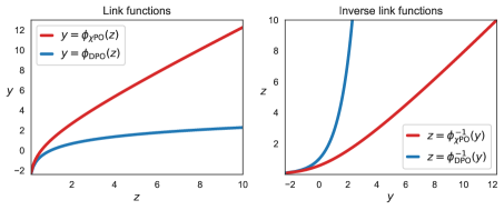
Figure 1: Behavior of the mixed $\chi^{2}$-regularization link function $\phi_{\texttt{$\chi$PO}}(z)=z+\log{}z$ and inverse $\phi_{\texttt{$\chi$PO}}^{-1}(z)=W_{0}(\exp(z))$, compared to the KL-regularization link function $\phi_{\texttt{DPO}}(z)=\log{}z$ and inverse $\phi_{\texttt{DPO}}^{-1}(z)=\exp(z)$. $\phi_{\texttt{$\chi$PO}}^{-1}(z)\approx z$ for $z\geq 1$, leading to favorable heavy-tailed, pessimistic behavior.

4.2 The Bias-Overoptimization Tradeoff

We are now well equipped to understand how $\chi$PO modulates the tradeoff between overoptimization and bias using the regularization parameter $\beta$, and how this tradeoff compares to vanilla DPO. To showcase this, we take a reward modeling perspective, and consider the setting in which the policy class $\Pi$ is induced by a given reward model class $\mathcal{R}$, similar to Example 3.1.

Suppose we start with a reward model class $\mathcal{R}\subset(\mathcal{X}\times\mathcal{A}\to[0,R_{\mathsf{max}}])$ such that $r^{\star}\in\mathcal{R}$. If we use the induced policy class

$$\Pi_{\textsf{DPO},\beta}\vcentcolon={}\left\{\pi(a\mid{}x)=\pi_{\mathsf{ref}}(a\mid{}x)\cdot\exp(\beta^{-1}(r(x,a)-Z_{\beta,r;\mathsf{KL}}(x)))\mid{}r\in\mathcal{R}\right\},$$ (17)

then DPO can be interpreted as fitting a reward model ${\widehat{r}}$ using maximum likelihood (Eq. 3) and then outputting the policy $\widehat{\pi}_{\textsf{DPO}}(a\mid{}x)=\pi_{\mathsf{ref}}(a\mid{}x)\cdot\exp(\beta^{-1}({\widehat{r}}(x,a)-Z_{\beta,{\widehat{r}};\mathsf{KL}}(x)))$. Meanwhile, if we use the induced policy class

$$\Pi_{\textsf{{$\chi$PO}},\beta}\vcentcolon={}\left\{\pi(a\mid{}x)=\pi_{\mathsf{ref}}(a\mid{}x)\cdot\phi^{-1}(\beta^{-1}(r(x,a)-Z_{\beta,r}(x)))\mid{}r\in\mathcal{R}\right\},$$ (18)

then $\chi$PO can be interpreted as fitting a reward model ${\widehat{r}}$ with the exact same maximum likelihood objective, but instead outputting the policy $\widehat{\pi}_{\textsf{{$\chi$PO}}}(a\mid{}x)=\pi_{\mathsf{ref}}(a\mid{}x)\cdot\phi^{-1}(\beta^{-1}({\widehat{r}}(x,a)-Z_{\beta,{\widehat{r}}}(x)))$.

The policies $\widehat{\pi}_{\textsf{{$\chi$PO}}}$ and $\widehat{\pi}_{\textsf{{DPO}}}$ are induced by the same reward model ${\widehat{r}}$, and both use the parameter $\beta$ to balance bias and overoptimization. For both policies, large $\beta$ means the policy avoids overfitting to errors in the reward model (the extreme case is $\beta\to\infty$, in which case both policies become $\pi_{\mathsf{ref}}$), while small $\beta$ means the policy has low bias, i.e., low error in the case where the model is correct in the sense that ${\widehat{r}}=r^{\star}$ (the extreme case is $\beta\to{}0$, in which case both policies become $x\mapsto\mathop{\mathrm{argmax}}_{a:\pi_{\mathsf{ref}}(a\mid{}x)>0}{\widehat{r}}(x,a)$). Yet, for the same choice of $\beta$, $\widehat{\pi}_{\textsf{{$\chi$PO}}}$ is significantly more heavy-tailed than $\widehat{\pi}_{\textsf{DPO}}$, a consequence of the pessimism induced by $\chi^{2}$-regularization; see Fig. 2, which plots the action distribution for both policies as a function of $\beta$.

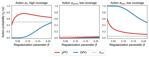
Figure 2: Action probabilities for policies learned by $\chi$PO and DPO on the example from Section 4.3, under the “bad” event $\mathcal{E}$ in which the true reward model is $r^{\star}=r_{1}$ but the estimated reward model is ${\widehat{r}}=r_{2}$ ($n=10$). Here, $r^{\star}(a_{\mathsf{good}})=1$ and $r^{\star}(a_{\mathsf{bad}})=0$, but ${\widehat{r}}(a_{\mathsf{good}})=0$ and ${\widehat{r}}(a_{\mathsf{good}})=1$; both reward functions have $r^{\star}(a_{0})={\widehat{r}}(a_{0})=1/2$, and the goal is to compete with a comparator policy that deterministically plays $a_{0}$.
Overoptimization. The DPO policy is greedier with respect to the incorrect reward model and places much larger mass on the bad action $a_{\mathsf{bad}}$ for all $\beta\in(0,\frac{1}{2\log n}]$ (Right). As a result, the DPO policy places much smaller mass on the baseline action $a_{0}$, suffering significantly more overoptimization error compared to $\chi$PO (Left; see also Fig. 3).
Bias. Compared to DPO, $\chi$PO has a higher probability of taking the optimal action $a_{\mathsf{good}}$, and thus has lower bias (Center). As a result, it strikes a better better bias-overoptimization tradeoff than DPO, and is competitive with respect to the comparator $a_{0}$ even when DPO fails to converge.

4.3 An Illustrative Example

We now give a concrete example in which $\chi$PO allows the user to tune $\beta$ to achieve tight statistical rates, yet no choice of $\beta$ for DPO leads to comparable performance (effectively, any choice of $\beta$ is either susceptible to overoptimization, or has unacceptably high bias). This illustrates the favorable tradeoff between bias and overoptimization achieved by $\chi$PO.

Let $n\in\mathbb{N}$ with $n\geq{}2$ be given. We consider a problem instance with $\mathcal{X}=\{\varnothing\}$ and $\mathcal{A}=\left\{a_{0},a_{1},a_{2},a_{3}\right\}$. We define $\pi_{\mathsf{ref}}$ via

$$\pi_{\mathsf{ref}}(a_{0})=\tfrac{1}{2},\quad\pi_{\mathsf{ref}}(a_{1})=\pi_{\mathsf{ref}}(a_{2})=\tfrac{1}{2n},\quad\text{and}\quad\pi_{\mathsf{ref}}(a_{3})=\tfrac{n-2}{2n}.$$

We define a reward class with two reward functions $\mathcal{R}:=\{r_{1},r_{2}\}$ as follows. For $i\in\{1,2\}$:

$$r_{i}(a_{0})=1/2,\quad r_{i}(a_{i})=1,\quad r_{i}(a_{j})=0,\;\;\forall j\neq i.$$

Let $\beta>0$ be fixed. To compare $\chi$PO and DPO, we consider their behavior when invoked with the induced policy classes $\Pi_{\textsf{{$\chi$PO}},\beta}$ and $\Pi_{\textsf{DPO},\beta}$ defined above. Recall that with this choice, the two algorithms can be interpreted as fitting a reward model ${\widehat{r}}$ using maximum likelihood (Eq. 3) and returning the policies $\widehat{\pi}_{\textsf{{$\chi$PO}}}(a\mid{}x)=\pi_{\mathsf{ref}}(a\mid{}x)\cdot\phi^{-1}(\beta^{-1}({\widehat{r}}(x,a)-Z_{\beta,{\widehat{r}}}(x)))$ and $\widehat{\pi}_{\textsf{DPO}}(a\mid{}x)=\pi_{\mathsf{ref}}(a\mid{}x)\cdot\exp(\beta^{-1}({\widehat{r}}(x,a)-Z_{\beta,{\widehat{r}};\mathsf{KL}}(x)))$, respectively.

Suppose that $r_{1}$ is the true reward function. It is hopeless (information-theoretically) to compete with the unconstrained optimal action $a_{1}$, as we are in a sample-starved regime where $\mathcal{C}^{a_{1}}=2n$ (in the language of Eq. 13). Indeed, one can show (see proof of Proposition A.1 in Appendix A) that with constant probability, none of the examples in the offline dataset $\mathcal{D}_{\mathsf{pref}}$ contain actions $a_{1}$ or $a_{2}$. Under this event, which we denote by $\mathcal{E}$, the value for the maximum likelihood objective in Eq. 3 is identical for $r_{1}$ and $r_{2}$, so we may obtain ${\widehat{r}}=r_{2}$ (due to adversarial tie-breaking). However, in spite of the fact that the policies $\widehat{\pi}_{\textsf{{$\chi$PO}}}$ and $\widehat{\pi}_{\textsf{DPO}}$ are induced by the same (incorrect) reward function ${\widehat{r}}=r_{2}$, they produce very different action distributions, as highlighted in Fig. 2.

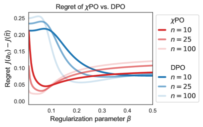
Figure 3: The regret $J(a_{0})-J(\widehat{\pi})$ in the construction from Proposition A.1 for different values of $n$. We again condition on the “bad” event $\mathcal{E}$ where ${\widehat{r}}=r_{2}\neq r^{\star}$. For each $n$, the error from overoptimization dominates when $\beta\leq(2\log n)^{-1}$ (as discussed in Section 4.3), and the error from bias dominates when $\beta>(2\log n)^{-1}$. Taking the best choice of $\beta$ for each method, DPO converges at an exponentially slower rate than $\chi$PO (see Proposition A.1 for formal statement).

To understand this, note that even in the sample-starved regime, we can still hope to compete with the “baseline” action $a_{0}$; Fig. 3 shows that $\chi$PO has low regret against this action, while DPO has high regret. In particular, since $\mathcal{C}^{a_{0}}=2$, Theorem 3.1 (Eq. 13) implies that $\chi$PO achieves

$$J(a_{0})-J(\widehat{\pi}_{\textsf{{$\chi$PO}}})\lesssim{}\sqrt{\frac{1}{n}}+\beta+\beta^{-1}\frac{1}{n},$$

and setting $\beta\propto\sqrt{\frac{1}{n}}$ leads to $J(a_{0})-J(\widehat{\pi}_{\textsf{{$\chi$PO}}})\lesssim{}\sqrt{\frac{1}{n}}$. This is a consequence of the pessimistic, heavy-tailed nature of $\widehat{\pi}_{\textsf{{$\chi$PO}}}$ (cf. Proposition 4.2), which places no more than $\beta^{-1}/n$ probability mass on the (incorrect) greedy action $a_{2}$ for ${\widehat{r}}=r_{2}$, thereby correctly capturing the inherent uncertainty in the reward for this action.

On the other hand, it is straightforward to show that for all possible values $\beta\leq{}(2\log{}n)^{-1}$, the DPO policy $\widehat{\pi}_{\textsf{{DPO}}}$ has regret

$$J(a_{0})-J(\widehat{\pi}_{\textsf{{DPO}}})\geq{}\frac{1}{2}\left(1-\frac{1}{1+\frac{1}{n}e^{\frac{1}{2}}+(1-\frac{1}{n})e^{-\frac{1}{2\beta}}}\right)-\frac{1}{2n}\geq\Omega(1)$$

whenever $n\geq{}2$. This is because when $\beta\leq(2\log{}n)^{-1}$, $\widehat{\pi}_{\textsf{{DPO}}}$ assigns excessively high probability to the incorrect greedy action $a_{2}$, an instance of overoptimization. Meanwhile, larger choices for $\beta$ lead to excessively large bias in general (see Section A.1 for a more sophisticated construction which extends this lower bound to all possible $\beta$). In other words, as illustrated in Fig. 3, no choice of $\beta$ gives a favorable tradeoff between overoptimization and bias.

To summarize, for DPO, large values of $\beta$ are required to avoid overfitting to the reward function, incurring high bias. Meanwhile, $\chi$PO avoids overoptimization using comparatively small values for $\beta$, yet has bias no worse than that of DPO, thereby striking a better tradeoff. We mention that the “DPO+SFT” algorithm of Liu et al. (2024); Cen et al. (2024); Fisch et al. (2024) also fails on the construction above; see Proposition A.1 in Section A.1 for details.

Remark 4.1 (DPO decreases probabilities of preferred and rejected responses).

Various recent works have noted an empirical phenomenon in which DPO decreases the probabilities for both preferred and rejected responses throughout training (Yuan et al., 2024; Pal et al., 2024; Rafailov et al., 2024b). Interestingly, we observe that the example above exhibits this phenomenon. Notably, if $\beta<(2\log{}n)^{-1}$, then under the event $\mathcal{E}$ in which the offline dataset $\mathcal{D}_{\mathsf{pref}}$ does not contain the actions $a_{1}$ or $a_{2}$ (so that ${\widehat{r}}=r_{2}$), we observe that $\widehat{\pi}_{\textsf{DPO}}(a_{0})=\frac{\frac{1}{2}e^{\frac{1}{2\beta}}}{\frac{1}{2}e^{\frac{1}{2\beta}}+\frac{1}{2n}e^{\frac{1}{\beta}}+\frac{n-1}{2n}}<\frac{1}{2}=\pi_{\mathsf{ref}}(a_{0})$, and for all $i>2$, $\widehat{\pi}_{\textsf{DPO}}(a_{i})=\frac{\frac{1}{2n}}{\frac{1}{2}e^{\frac{1}{2\beta}}+\frac{1}{2n}e^{\frac{1}{\beta}}+\frac{n-1}{2n}}<\frac{1}{2n}=\pi_{\mathsf{ref}}(a_{i})$. We conclude that for all $a\in\mathcal{D}_{\mathsf{pref}}$,

$$\widehat{\pi}_{\textsf{DPO}}(a)<\pi_{\mathsf{ref}}(a).$$

We emphasize that this behavior arises due to the use of function approximation. When the reward class $\mathcal{R}$ (equivalently, the policy class $\Pi_{\textsf{DPO},\beta}$) is restricted, the algorithm can aggressively (and incorrectly) extrapolate rewards for actions outside the dataset and, in doing so, inadvertently decrease the probabilities for preferred responses in the dataset. Meanwhile, in the same parameter range, $\chi$PO satisfies (see Fig. 2)

$$\widehat{\pi}_{\textsf{{$\chi$PO}}}(a_{0})>\pi_{\mathsf{ref}}(a_{0}),$$

highlighting that pessimism can mitigate this phenomenon.

4.4 Nontriviality and Role of $V_{\mathsf{max}}$ Parameter

To close this section, we discuss the role of the $V_{\mathsf{max}}$ parameter (Assumption 3.2) used in the analysis of $\chi$PO (Theorem 3.1) in depth, motivating it from the perspective of the induced policy class $\Pi_{\textsf{{$\chi$PO}},\beta}$ from Section 4.2.

Assumption 3.2 effectively implies that all policies $\pi\in\Pi$ satisfy $\big{\|}\frac{\pi}{\pi_{\mathsf{ref}}}\big{\|}_{\infty}\lesssim\frac{V_{\mathsf{max}}}{\beta}$; in other words, the policy class we use in $\chi$PO satisfies all-policy $L_{\infty}$-concentrability with $\max_{\pi\in\Pi}\mathcal{C}^{\pi}_{\infty}\lesssim\frac{V_{\mathsf{max}}}{\beta}$. This might seem to trivialize the offline alignment problem at first glance, since it would suffice to prove a generalization guarantee based on all-policy concentrability, and then plug this bound in. We will show that this is not the case, and that this is actually an intrinsic feature of $\chi^{2}$-regularization.

In more detail, recall that for $\chi$PO, we require the realizability assumption that $\pi^{\star}_{{\scriptscriptstyle\beta}}\in\Pi$ (Assumption 3.1), where $\pi^{\star}_{{\scriptscriptstyle\beta}}$ is the optimal mixed $\chi^{2}$-regularized policy that satisfies $r^{\star}(x,a)=\beta\phi\left(\frac{\pi^{\star}_{{\scriptscriptstyle\beta}}(a\mid{}x)}{\pi_{\mathsf{ref}}(a\mid{}x)}\right)+Z_{\beta,r^{\star}}(x)$. This policy, via Proposition 4.2, satisfies $\big{\|}\frac{\pi^{\star}_{{\scriptscriptstyle\beta}}}{\pi_{\mathsf{ref}}}\big{\|}_{\infty}\lesssim\frac{R_{\mathsf{max}}}{\beta}$, so from a statistical perspective, we can take Assumption 3.2 to hold without loss of generality by removing any policy that violates this bound. In addition, as highlighted by Example 3.1, if we begin from a class of bounded reward models $\mathcal{R}$ with $r^{\star}\in\mathcal{R}$, Assumption 3.2 holds with $V_{\mathsf{max}}\lesssim{}R_{\mathsf{max}}$ for the induced class $\Pi_{\textsf{{$\chi$PO}},\beta}$ defined in Eq. 18, even though knowledge of such a reward model class is a mild statistical assumption that clearly does not trivialize the learning problem.

On the other hand, for DPO, a minimal assumption is that $\pi^{\star}_{\beta;\mathsf{KL}}\in\Pi$ (Xie et al., 2024), where $\pi^{\star}_{\beta;\mathsf{KL}}$ is the optimal KL-regularized policy that satisfies $r^{\star}(x,a)=\beta\log\frac{\pi^{\star}_{\beta;\mathsf{KL}}(a\mid{}x)}{\pi_{\mathsf{ref}}(a\mid{}x)}+Z_{\beta,r^{\star};\mathsf{KL}}(x)$. Unlike the optimal mixed $\chi^{2}$-regularized policy, $\pi^{\star}_{\beta;\mathsf{KL}}$ has $\frac{\pi^{\star}_{\beta;\mathsf{KL}}(a\mid{}x)}{\pi_{\mathsf{ref}}(a\mid{}x)}\gtrsim{}\exp\left(\frac{R_{\mathsf{max}}}{\beta}\right)$. This means that it is impossible to find a policy class that simultaneously (1) realizes $\pi^{\star}_{\beta;\mathsf{KL}}$, and (2) satisfies all-policy concentrability with $\max_{\pi\in\Pi}\mathcal{C}^{\pi}_{\infty}\ll{}\exp\left(\frac{R_{\mathsf{max}}}{\beta}\right)$. As the bias of DPO is unacceptably large unless $\beta=\mathrm{poly}(1/n)$ (the “small-$\beta$” regime), this leads to vacuous guarantees.

In view of these observations, our analysis of $\chi$PO can be interpreted as (implicitly) showing that for any bounded reward class $\mathcal{R}$, there exists a policy class $\Pi$ (precisely, the class $\Pi_{\textsf{{$\chi$PO}},\beta}$ defined in Eq. 18) such that the following properties hold:

1. Bounded bias. For every $r\in\mathcal{R}$, there exists $\pi_{r}\in\Pi$ such that for all policies $\pi^{\star}$, $J_{r}(\pi^{\star})-J_{r}(\pi_{r})\lesssim{}\beta\cdot\mathcal{C}^{\pi^{\star}}$.

2. Bounded overoptimization. For all $\pi\in\Pi$, $\big{\|}\frac{\pi}{\pi_{\mathsf{ref}}}\big{\|}_{\infty}\lesssim\frac{R_{\mathsf{max}}}{\beta}$.

We view this as an interesting and non-trivial contribution in its own right. We mention in passing that while it is indeed possible to analyze $\chi$PO by first proving a sample complexity guarantee based on all-policy concentrability and then using that $\max_{\pi\in\Pi}\mathcal{C}^{\pi}_{\infty}\lesssim\frac{V_{\mathsf{max}}}{\beta}$, this would lead to a loose bound relative to Theorem 3.1.

5 Analysis of $\boldsymbol{\chi}$PO: Proof Sketch for thm:main

In this section, we sketch the proof of the main guarantee for $\chi$PO, Theorem 3.1, with the full proof deferred to Appendix E. A central object in the proof is the implicit reward model induced by the $\chi$PO policy $\widehat{\pi}$, which we define via

$${\widehat{r}}(x,a)\vcentcolon={}\beta\phi{}\left(\frac{\widehat{\pi}(a\mid{}x)}{\pi_{\mathsf{ref}}(a\mid{}x)}\right).$$ (19)

As we will show, this reward model is a natural bridge between $\chi$PO and the corresponding mixed $\chi^{2}$-regularized RLHF objective in Section 3.1, and allows us to view $\chi$PO from a reward-based perspective. In particular, note that if we analogously define an induced reward model class $\mathcal{R}_{\Pi}\vcentcolon={}\{r(x,a)=\beta\phi{}\left(\frac{\pi(a\mid{}x)}{\pi_{\mathsf{ref}}(a\mid{}x)}\right):\pi\in\Pi\}$, then 3 of $\chi$PO can be viewed as performing maximum likelihood estimation over this class (in the sense of Eq. 3) under the Bradley-Terry model. Under Assumption 3.1, $\mathcal{R}_{\Pi}$ realizes the true reward function $r$ up to an action-independent shift. As a result, if we define $\Delta^{{r}}(x,a,b)\vcentcolon={}r(x,a)-r(x,b)$, then using a fairly standard generalization bound for maximum likelihood estimation (e.g., Wong and Shen (1995); Zhang (2006); de Geer (2000); see Lemma E.1), we can show that

$$\varepsilon_{\mathrm{stat}}^{2}\vcentcolon={}\operatorname{\mathbb{E}}_{x\sim\rho,a\sim\pi_{\mathsf{ref}},b\sim\pi_{\mathsf{ref}}}\left[\left\lvert\Delta^{{{\widehat{r}}}}(x,a,b)-\Delta^{{r^{\star}}}(x,a,b)\right\rvert^{2}\right]\leq O\left(V_{\mathsf{max}}e^{2R_{\mathsf{max}}}\cdot\frac{\log(|\Pi|/\delta)}{n}\right).$$ (20)

In other words, the estimated reward model ${\widehat{r}}$ is accurate under the action distribution induced by $\pi_{\mathsf{ref}}$. However, ${\widehat{r}}$ may still be inaccurate for policies that select different actions from $\pi_{\mathsf{ref}}$, raising concerns of overoptimization. To address this issue, we use the following lemma, which shows that $\chi^{2}$-divergence bounds the extent to which the accuracy of a reward model ${\widehat{r}}$ trained under $\pi_{\mathsf{ref}}$ will transfer to a downstream policy $\pi$ of interest; this will motivate our use of $\chi^{2}$-regularization.

Lemma 5.1 (Informal version of Lemma E.3).

For any policy $\pi:\mathcal{X}\to\Delta(\mathcal{A})$, it holds that

$$\operatorname{\mathbb{E}}_{x\sim\rho,a\sim\pi(\cdot\mid{}x),b\sim\pi_{\mathsf{ref}}(\cdot\mid{}x)}\left[\left\lvert\Delta^{{{\widehat{r}}}}(x,a,b)-\Delta^{{r^{\star}}}(x,a,b)\right\rvert\right]\lesssim\sqrt{(1+D_{\chi^{2}}\left(\pi\;\|\;{}\pi_{\mathsf{ref}}\right))\cdot\varepsilon_{\mathrm{stat}}^{2}}.$$

Going forward, let us abbreviate $\operatorname{\mathbb{E}}_{\pi,\pi_{\mathsf{ref}}}\left[\cdot\right]=\operatorname{\mathbb{E}}_{x\sim\rho,a\sim\pi(\cdot\mid{}x),b\sim\pi_{\mathsf{ref}}(\cdot\mid{}x)}\left[\cdot\right]$. Let $\pi^{\star}$ be an arbitrary policy. Noting that $\mathcal{C}^{\pi}=1+2D_{\chi^{2}}\left(\pi\;\|\;{}\pi_{\mathsf{ref}}\right)$ and that

$$J(\pi^{\star})-J(\widehat{\pi})\lesssim{}\operatorname{\mathbb{E}}_{\pi^{\star},\pi_{\mathsf{ref}}}\left[\left\lvert\Delta^{{{\widehat{r}}}}(x,a,b)-\Delta^{{r^{\star}}}(x,a,b)\right\rvert\right]+\operatorname{\mathbb{E}}_{\widehat{\pi},\pi_{\mathsf{ref}}}\left[\left\lvert\Delta^{{{\widehat{r}}}}(x,a,b)-\Delta^{{r^{\star}}}(x,a,b)\right\rvert\right],$$

it follows immediately from Lemma 5.1 that $\chi$PO obtains a crude guarantee scaling with all-policy concentrability, i.e. $J(\pi^{\star})-J(\widehat{\pi})\lesssim{}\sqrt{(\mathcal{C}^{\pi^{\star}}+\mathcal{C}^{\widehat{\pi}})\varepsilon_{\mathrm{stat}}^{2}}\leq\sqrt{(\mathcal{C}^{\pi^{\star}}+\max_{\pi\in\Pi}\mathcal{C}^{\pi})\varepsilon_{\mathrm{stat}}^{2}}$. This inequality is tight for non-pessimistic algorithms like DPO, which reflects their sensitivity to overoptimization. To obtain the improved guarantee for $\chi$PO in Theorem 3.1, which scales only with single-policy concentrability $\mathcal{C}^{\pi^{\star}}$, the crux of the remaining proof will be to show that $\chi$PO implicitly implements pessimism via mixed $\chi^{2}$-regularization. For this, we appeal to the following central technical lemma, which we expect to find broader use.

Lemma 5.2 (Informal version of Lemma E.2).

Let $f$ be a convex function with $\mathrm{dom}(f)=\mathbb{R}_{+}$ that is differentiable over its domain. Given any parameter $\beta>0$ and policy $\bar{\pi}:\mathcal{X}\rightarrow\Delta(\mathcal{A})$ with $\bar{\pi}(a\mid{}x)\in\mathrm{dom}(f^{\prime})$ for all $x,a$, define the reward model $\bar{r}(x,a)=\beta f^{\prime}\left(\frac{\macc@depth\char 1\relax\frozen@everymath{\macc@group}\macc@set@skewchar\macc@nested@a 111{}(a|x)}{\pi_{\mathsf{ref}}(a|x)}\right)$. Then

$$\bar{\pi}\in\mathop{\mathrm{argmax}}_{\pi}{}\operatorname{\mathbb{E}}_{\pi}\left[\bar{r}(x,a)\right]-\beta\cdot D_{f}\left(\pi\,\|\,\pi_{\mathsf{ref}}\right).$$

Under Assumption 3.2 we have $\widehat{\pi}\in\mathrm{dom}(f_{\chi_{\textsf{mix}}}^{\prime})$. Then recalling that ${\widehat{r}}(x,a)\vcentcolon={}\beta\phi{}\left(\frac{\widehat{\pi}(a\mid{}x)}{\pi_{\mathsf{ref}}(a\mid{}x)}\right)=\beta f_{\chi_{\textsf{mix}}}^{\prime}\left(\frac{\widehat{\pi}(a\mid{}x)}{\pi_{\mathsf{ref}}(a\mid{}x)}\right)$ and that $f_{\chi_{\textsf{mix}}}$ is convex, Lemma 5.2 implies that the policy $\widehat{\pi}$ produced by $\chi$PO satisfies

$$\widehat{\pi}\in\mathop{\mathrm{argmax}}_{\pi\in\Pi}J_{\beta,{\widehat{r}}}^{\chi_{\textsf{mix}}}(\pi)\vcentcolon={}\operatorname{\mathbb{E}}_{\pi}\left[{\widehat{r}}\right]-\beta D_{\chi^{2}}\left(\pi\;\|\;{}\pi_{\mathsf{ref}}\right)-\beta D_{\mathsf{KL}}\left(\pi\,\|\,\pi_{\mathsf{ref}}\right).$$ (21)

In other words,

The $\chi$PO policy $\widehat{\pi}$ optimizes the mixed $\chi^{2}$-regularized RLHF objective under its own implicit reward model.

This formally justifies the claim that $\chi$PO implicitly implements pessimism via $\chi^{2}$-regularization. With this result in hand, we are now ready to prove Theorem 3.1. Let $\pi^{\star}$ be an arbitrary policy. Since $J_{\beta,{\widehat{r}}}^{\chi_{\textsf{mix}}}(\widehat{\pi})\geq J_{\beta,{\widehat{r}}}^{\chi_{\textsf{mix}}}(\pi^{\star})$ by Eq. 21, we can decompose the regret $J(\pi^{\star})-J(\widehat{\pi})$ as

$$J(\pi^{\star})-J(\widehat{\pi})\leq ~{}J(\pi^{\star})-J_{\beta,{\widehat{r}}}^{\chi_{\textsf{mix}}}(\pi^{\star})+J_{\beta,{\widehat{r}}}^{\chi_{\textsf{mix}}}(\widehat{\pi})-J(\widehat{\pi})$$

$$= ~{}\underbrace{J(\pi^{\star})-J(\pi_{\mathsf{ref}})-J_{\beta,{\widehat{r}}}^{\chi_{\textsf{mix}}}(\pi^{\star})+J_{\beta,{\widehat{r}}}^{\chi_{\textsf{mix}}}(\pi_{\mathsf{ref}})}_{\text{(I)}}+\underbrace{J_{\beta,{\widehat{r}}}^{\chi_{\textsf{mix}}}(\widehat{\pi})-J_{\beta,{\widehat{r}}}^{\chi_{\textsf{mix}}}(\pi_{\mathsf{ref}})-J(\widehat{\pi})+J(\pi_{\mathsf{ref}})}_{\text{(II)}}.$$

In the second line, we have added or subtracted the baselines $J(\pi_{\mathsf{ref}})$ and $J_{\beta,{\widehat{r}}}^{\chi_{\textsf{mix}}}(\pi_{\mathsf{ref}})$ to center the objectives with the performance of the reference policy. Up to statistical errors, the first term (I) corresponds to error from how much $J_{\beta,{\widehat{r}}}^{\chi_{\textsf{mix}}}(\pi^{\star})$ underestimates the return of $\pi^{\star}$ (bias), and the second term (II) corresponds to error from how much $J_{\beta,{\widehat{r}}}^{\chi_{\textsf{mix}}}(\widehat{\pi})$ overestimates the return of $\widehat{\pi}$ (overoptimization). As we will see shortly, these two sources of error are directly controlled (in opposing ways) by the strength of the regularization parameter $\beta$ in Eq. 21.

First, expanding the definition of $J_{\beta,{\widehat{r}}}^{\chi_{\textsf{mix}}}(\pi^{\star})$ and centering the returns using the reference policies, we have

(I) $$=J(\pi^{\star})-J_{\beta,{\widehat{r}}}^{\chi_{\textsf{mix}}}(\pi^{\star})-J(\pi_{\mathsf{ref}})+J_{\beta,{\widehat{r}}}^{\chi_{\textsf{mix}}}(\pi_{\mathsf{ref}})$$

$$=\operatorname{\mathbb{E}}_{\pi^{\star}}\left[r^{\star}(x,a)\right]-\operatorname{\mathbb{E}}_{\pi^{\star}}\left[{\widehat{r}}(x,a)\right]+\beta D_{\chi^{2}}\left(\pi^{\star}\;\|\;{}\pi_{\mathsf{ref}}\right)+\beta D_{\mathsf{KL}}\left(\pi^{\star}\,\|\,\pi_{\mathsf{ref}}\right)-\operatorname{\mathbb{E}}_{\widehat{\pi}}[r^{\star}(x,a)]+\operatorname{\mathbb{E}}_{\pi_{\mathsf{ref}}}[{\widehat{r}}(x,a)]$$

$$=\operatorname{\mathbb{E}}_{\pi^{\star},\pi_{\mathsf{ref}}}[\Delta^{{r^{\star}}}(x,a,b)-\Delta^{{{\widehat{r}}}}(x,a,b)]+\beta D_{\chi^{2}}\left(\pi^{\star}\;\|\;{}\pi_{\mathsf{ref}}\right)+\beta D_{\mathsf{KL}}\left(\pi^{\star}\,\|\,\pi_{\mathsf{ref}}\right)$$

$$\leq\sqrt{(1+D_{\chi^{2}}\left(\pi^{\star}\;\|\;{}\pi_{\mathsf{ref}}\right))\cdot\varepsilon_{\mathrm{stat}}^{2}}+{}\underbrace{\beta\cdot D_{\chi^{2}}\left(\pi^{\star}\;\|\;{}\pi_{\mathsf{ref}}\right)}_{\text{bias}}.$$

Above, we have used that $D_{\mathsf{KL}}\left(\pi\,\|\,\pi_{\mathsf{ref}}\right)\leq D_{\chi^{2}}\left(\pi\;\|\;{}\pi_{\mathsf{ref}}\right)$ for any policy $\pi$, along with the bound on reward estimation error from Lemma 5.1. Next, expanding $J_{\beta,{\widehat{r}}}^{\chi_{\textsf{mix}}}(\widehat{\pi})$ and centering the returns in a similar fashion,

(II) $$=J_{\beta,{\widehat{r}}}^{\chi_{\textsf{mix}}}(\widehat{\pi})-J(\widehat{\pi})-J_{\beta,{\widehat{r}}}^{\chi_{\textsf{mix}}}(\pi_{\mathsf{ref}})+J(\pi_{\mathsf{ref}})$$

$$=\operatorname{\mathbb{E}}_{\widehat{\pi},\pi_{\mathsf{ref}}}[\Delta^{{{\widehat{r}}}}(x,a,b)-\Delta^{{r^{\star}}}(x,a,b)]-\beta D_{\chi^{2}}\left(\widehat{\pi}\;\|\;{}\pi_{\mathsf{ref}}\right)-\beta D_{\mathsf{KL}}\left(\widehat{\pi}\,\|\,\pi_{\mathsf{ref}}\right)$$

$$\leq\sqrt{(1+D_{\chi^{2}}\left(\widehat{\pi}\;\|\;{}\pi_{\mathsf{ref}}\right))\cdot\varepsilon_{\mathrm{stat}}^{2}}-\beta\cdot D_{\chi^{2}}\left(\widehat{\pi}\;\|\;{}\pi_{\mathsf{ref}}\right)$$

$$\lesssim{}\varepsilon_{\mathrm{stat}}+\underbrace{\beta^{-1}\varepsilon_{\mathrm{stat}}^{2}}_{\textrm{overoptimization error}}.$$

Above, the first inequality uses $D_{\mathsf{KL}}\left(\pi\,\|\,\pi_{\mathsf{ref}}\right)\geq{}0$ and Lemma 5.1, while the second inequality uses AM-GM. Critically, by using $\chi^{2}$-regularization, we are able to cancel the on-policy error term $\sqrt{(1+D_{\chi^{2}}\left(\widehat{\pi}\;\|\;{}\pi_{\mathsf{ref}}\right))\cdot\varepsilon_{\mathrm{stat}}^{2}}$ that arises from change-of-measure, leading to a modest $\beta^{-1}\varepsilon_{\mathrm{stat}}^{2}$ penalty for overoptimization.

Combining these results, and recalling that $\mathcal{C}^{\pi}=1+2D_{\chi^{2}}\left(\pi\;\|\;{}\pi_{\mathsf{ref}}\right)$, we conclude that

$$J(\pi^{\star})-J(\widehat{\pi})\lesssim{}\sqrt{\mathcal{C}^{\pi^{\star}}\cdot\varepsilon_{\mathrm{stat}}^{2}}+\underbrace{\beta\cdot\mathcal{C}^{\pi^{\star}}}_{\textrm{bias}}+\underbrace{\beta^{-1}\cdot\varepsilon_{\mathrm{stat}}^{2}}_{\textrm{overoptimization error}}.$$

The bias and overoptimization errors above arise from how well our chosen uncertainty quantifier, $\beta D_{\chi^{2}}\left(\pi\;\|\;{}\pi_{\mathsf{ref}}\right)$, accounts for the on-policy statistical error $\sqrt{(1+D_{\chi^{2}}\left(\pi\;\|\;{}\pi_{\mathsf{ref}}\right))\cdot\varepsilon_{\mathrm{stat}}^{2}}$ arising from Lemma 5.1; this is controlled by the magnitude of the regularization parameter $\beta$. When $\beta$ is too large, the uncertainty quantifier is overly pessimistic about the quality of the reward model ${\widehat{r}}$ under $\pi^{\star}$, which increases the bias of $\chi$PO. In contrast, the overoptimization error increases when $\beta$ is too small. In this regime, $\widehat{\pi}$ overfits to ${\widehat{r}}$ because the regularizer under-evaluates the statistical error of the learned policy. In order to obtain tight statistical rates, the choice of regularization parameter $\beta$ must carefully balance its opposing effects on bias and overoptimization error. For a fixed $\pi^{\star}$, choosing $\beta\propto(\varepsilon_{\mathrm{stat}}^{2}/\mathcal{C}^{\pi^{\star}})^{1/2}$ results in the second claim in Theorem 3.1.

6 General Preference Models

whzblue

All of our results so far concern the Bradley-Terry model (Eq. 1), which, as highlighted in prior work, is somewhat restrictive. Thus, in this section, we turn our attention to offline alignment under a general preference model which does not assume transitivity (Munos et al., 2023; Wang et al., 2023b; Swamy et al., 2024; Rosset et al., 2024; Ye et al., 2024). The setup is the same as Section 2, but we assume that for a given context $x$ and pair of actions $(a,b)$, the preference $y\in\{0,1\}$ is generated via a Bernoulli Distribution

$$y\sim{}\mathrm{Ber}\left(\mathcal{P}^{\star}(a\succ b\mid{}x)\right),$$ (22)

where $\mathcal{P}^{\star}(a\succ b\mid{}x)\in[0,1]$ is a general preference distribution. For a pair of policies $\pi,\pi^{\prime}$, let $\mathcal{P}^{\star}(\pi\succ\pi^{\prime})\vcentcolon={}\operatorname{\mathbb{E}}_{x\sim\rho}\left[\mathcal{P}^{\star}(\pi(x)\succ{}\pi^{\prime}(x)\mid{}x)\right]$. Following Wang et al. (2023b); Munos et al. (2023); Swamy et al. (2024), we consider the minimax winner (Kreweras, 1965; Simpson, 1969; Kramer, 1973; Fishburn, 1984) or von Neumann winner (Dudík et al., 2015) as a solution concept:

$$\pi_{\mathsf{MW}}\vcentcolon={}\mathop{\mathrm{argmax}}_{\pi\in\Pi}\min_{\pi^{\prime}\in\Pi}\mathcal{P}^{\star}(\pi\succ{}\pi^{\prime}).$$

It will be useful to slightly reparameterize this formulation by introducing the preference function $\ell^{\star}(x,a,b)\vcentcolon={}2\mathcal{P}^{\star}(a\succ b\mid{}x)-1$. Note that for any well-defined preference model, we have $\mathcal{P}^{\star}(a\succ b\mid{}x)+\mathcal{P}^{\star}(b\succ a\mid{}x)=1$ for all $x,a,b$, which indicates that $\ell^{\star}$ satisfies skew symmetry:

$$\ell^{\star}(x,a,a)=0,\qquad\ell^{\star}(x,a,b)+\ell^{\star}(x,b,a)=0,\qquad\forall x\in\mathcal{X},a,b\in\mathcal{A}.$$

Furthermore, the minimax winner above is equivalent to

$$\pi_{\mathsf{MW}}\vcentcolon={}\mathop{\mathrm{argmax}}_{\pi\in\Pi}\min_{\pi^{\prime}\in\Pi}\ell^{\star}(\pi,\pi^{\prime}),$$ (23)

where $\ell^{\star}(\pi,\pi^{\prime}):=\mathbb{E}_{x\sim\rho,a\sim\pi(x),b\sim\pi^{\prime}(x)}[\ell^{\star}(x,a,b)]$. Concretely, our goal is to use the logged preference data $\mathcal{D}_{\mathsf{pref}}=\left\{(x,a_{+},a_{-})\right\}$ (with $(a_{+},a_{-})$ labeled according to Eq. 22) to compute a policy $\widehat{\pi}$ that is an $\varepsilon$-approximate minimax winner, in the sense that

$$\mathsf{DG}(\widehat{\pi})\vcentcolon={}\max_{\pi\in\Pi}\ell^{\star}(\pi,\widehat{\pi})-\min_{\pi\in\Pi}\ell^{\star}(\widehat{\pi},\pi)\leq\varepsilon.$$ (24)

6.1 Impossibility of Single-Policy Concentrability under General Preferences

While the general preference framework above is more powerful than the Bradley-Terry model, we now show that there is a statistical cost for this generality. In particular, our first result in this section shows that in contrast to the Bradley-Terry model, it is not possible to achieve sample complexity guarantees that scale with single-policy concentrability under general preferences, even when the learner has access to a small class of preference models $\mathscr{P}$ that contains the true preference model $\mathcal{P}$ (i.e., $\mathcal{P}^{\star}\in\mathscr{P}$).

Theorem 6.1 (Impossibility of single-policy concentrability under general preferences).

There exists two problem instances $\theta_{1}=(\rho,\mathcal{P}^{\star}_{1},\Pi)$ and $\theta_{2}=(\rho,\mathcal{P}^{\star}_{2},\Pi)$ differing only in their ground truth preference model, a data collection policy $\pi_{\mathsf{ref}}$, and a preference model class $\mathscr{P}=\{\mathcal{P}^{\star}_{1},\mathcal{P}^{\star}_{2}\}$ with $|\mathscr{P}|=2$ such that the following hold:

1. For both instances, the single-policy $L_{\infty}$-concentrability coefficient for a minimax winner is bounded: $\min_{\pi_{\mathsf{MW}}}\mathcal{C}_{\infty}^{\pi_{\mathsf{MW}}}\leq{}2$.

2. For any $n\in\mathbb{N}$ and any algorithm $\mathsf{Alg}$ which derives a policy $\widehat{\pi}$ from a dataset $\mathcal{D}_{\mathsf{pref}}$ of $n$ samples, there exists an instance $\theta\in\{\theta_{1},\theta_{2}\}$ such that $\pi_{\mathsf{ref}}$ incurs constant suboptimality:

   $$\min_{\mathsf{Alg}}\max_{i\in\{1,2\}}\operatorname{\mathbb{E}}_{\mathcal{D}_{\mathsf{pref}}\sim\theta_{i}}\left[\mathsf{DG}(\mathsf{Alg}(\mathcal{D}_{\mathsf{pref}});\theta_{i})\right]\geq{}\frac{1}{8},$$

   where $\mathsf{DG}(\pi;\theta)$ is the duality gap for policy $\pi$ on instance $\theta$.

This lower bound is inspired by similar results in the literature on offline RL in two-player zero-sum Markov games (Cui and Du, 2022). However, the lower bound constructions in Cui and Du (2022) cannot be directly applied as-is, because they do not satisfy the skew-symmetry property required by the general preference alignment framework. Our lower bound highlights that even under skew-symmetry, it is impossible to achieve single-policy concentrability for offline learning in two-player zero-sum games.

6.2 Iterative $\boldsymbol{\chi}$PO for General Preferences

In spite of the hardness in the prequel, we now show that an iterative variant of $\chi$PO—based on self-play—can learn a near-optimal minimax winner under the general preference model under a new local coverage condition—a condition that is stronger than the single policy concentrability but much weaker than global/all-policy concentrability and the notion of unilateral concentrability introduced by Cui and Du (2022).

Our algorithm, Iterative $\chi$PO, is described in Algorithm 2, and consists of two main steps.

Preference model estimation via least squares regression on $\mathcal{D}_{\mathsf{pref}}$

We first (3) learn a preference model from the offline preference dataset $\mathcal{D}_{\mathsf{pref}}$. We assume access to a preference function class $\mathcal{L}$ which is realizable in the sense that $\ell^{\star}\in\mathcal{L}$ and where all $\ell\in\mathcal{L}$ satisfy skew-symmetryc, and we will estimate $\ell^{\star}$ rather than $\mathcal{P}^{\star}$. We perform least-squares regression on $\mathcal{D}_{\mathsf{pref}}$ with $\mathcal{L}$ to learn $\ell^{\star}$:

$$\widehat{\ell}=\mathop{\mathrm{argmin}}_{\ell\in\mathcal{L}}\sum_{(x,a_{+},a_{-})\in\mathcal{D}_{\mathsf{pref}}}\left(\ell(x,a_{+},a_{-})-1\right)^{2}.$$

Policy optimization with iterative $\chi$PO update

Given the estimated model $\widehat{\ell}$, we compute an approximate minimax winner using an iterative regression scheme inspired by Gao et al. (2024). We proceed in $T$ iterations (5), where at each iteration $t$, we define an iteration-dependent reward function $\overline{r}^{t}(x,a)$ based on the current policy $\pi^{t}$ as

$$\overline{r}^{t}(x,a)=\mathbb{E}_{b\sim\pi^{t}(x)}[\widehat{\ell}(x,a,b)],\qquad\forall x\in\mathcal{X},a\in\mathcal{A}.$$

Then, for all $\pi,\pi^{\prime}\in\Pi$, we define a policy-dependent predictor $f^{\beta,\eta}_{\pi,\pi^{\prime}}(x,a,b)$, whose motivation will be described in detail momentarily, as follows:

$$f^{\beta,\eta}_{\pi,\pi^{\prime}}(x,a,b) :=\left(1+\frac{1}{\eta}\right)\cdot\left(\beta\phi\left(\frac{\pi\left(a\mid x\right)}{\pi_{\mathsf{ref}}\left(a\mid x\right)}\right)-\beta\phi\left(\frac{\pi\left(b\mid x\right)}{\pi_{\mathsf{ref}}\left(b\mid x\right)}\right)\right)$$

$$~{}~{}~{}~{}~{}~{}-\frac{1}{\eta}\left(\beta\phi\left(\frac{\pi^{\prime}\left(a\mid x\right)}{\pi_{\mathsf{ref}}\left(a\mid x\right)}\right)-\beta\phi\left(\frac{\pi^{\prime}\left(b\mid x\right)}{\pi_{\mathsf{ref}}\left(b\mid x\right)}\right)\right)$$ (25)

Using $f^{\beta,\eta}_{\pi,\pi^{t}}(x,a,b)$ as a policy-parameterized regression function, we (7) compute the next policy $\pi^{t+1}$ by solving a least-squares regression problem in which the Bayes optimal solution is the relative reward $\overline{r}^{t}(x,a)-\overline{r}^{t}(x,b)$ for iteration $t$.

Algorithm 2 Iterative $\chi$PO for General Preferences

1:Input: labeled preference dataset $\mathcal{D}_{\mathsf{pref}}$, preference model class $\mathcal{L}$, regularization coefficient $\beta$, stepsize $\eta$, total number of iterations $T$.

2:Initialize: $\pi^{1}=\pi_{\mathsf{ref}}$.

3:Learn a preference model $\widehat{\ell}$ via least-squares regression:

$$\widehat{\ell}=\mathop{\mathrm{argmin}}_{\ell\in\mathcal{L}}\sum_{(x,a_{+},a_{-})\in\mathcal{D}_{\mathsf{pref}}}\left(\ell(x,a_{+},a_{-})-1\right)^{2}.$$

4:Collect $m$ samples $\mathcal{D}_{\mathsf{x}}=\{(x,a,b)\}$ where each sample is drawn i.i.d. from $x\sim\rho,a\sim\pi_{\mathsf{ref}}(x),b\sim\pi_{\mathsf{ref}}(x)$.

5:for $t=1,\cdots,T$ do

6:     Sample $b_{t}\sim\pi^{t}(x)$ and let $\widehat{r}^{t}(x,a)=\widehat{\ell}(x,a,b_{t})$ for all $x\in\mathcal{X},a\in\mathcal{A}$.

7:     Compute

$$\pi^{t+1}=\mathop{\mathrm{argmin}}_{\pi\in\Pi}\sum_{(x,a,b)\in\mathcal{D}_{\mathsf{x}}}\left(\mathsf{clip}_{4}\left(f^{\beta,\eta}_{\pi,\pi^{t}}(x,a,b)\right)-(\widehat{r}^{t}(x,a)-\widehat{r}^{t}(x,b))\right)^{2},$$ (26)

       where $f^{\beta,\eta}_{\pi,\pi^{t}}(x,a,b)$ is defined in Eq. 25.

8:Output: $\widehat{\pi}={\sf unif}(\{\pi^{t}\}_{t=1}^{T})$.

Let us now explain the intuition behind the the predictor $f^{\beta,\eta}_{\pi,\pi^{\prime}}(x,a,b)$. Suppose that the regression step in 7 learns a predictor that can perfectly model the relative reward, i.e.,

$$\forall x,a,b,\quad f^{\beta,\eta}_{\pi^{t+1},\pi^{t}}(x,a,b)=\overline{r}^{t}(x,a)-\overline{r}^{t}(x,b),$$

In this case, we can show that the returned policy $\pi^{t+1}$ is the optimal policy for the following mixed $\chi^{2}$-regularized RL objective:

$$\pi^{t+1}(x)=\mathop{\mathrm{argmax}}_{p\in\Delta(\mathcal{X})}\left\{\operatorname{\mathbb{E}}_{a\sim{}p}\left[\overline{r}^{t}(x,a)\right]-\beta D_{f_{\chi_{\textsf{mix}}}}\left(p\,\|\,\pi_{\mathsf{ref}}(x)\right)-\frac{\beta}{\eta}B_{x}(p,\pi^{t})\right\},\qquad\forall x\in\mathcal{X},$$ (27)

where $B_{x}(p,\pi^{t})$ is the Bregman divergence induced by the regularizer $p\mapsto{}D_{f_{\chi_{\textsf{mix}}}}\left(p\,\|\,\pi_{\mathsf{ref}}(x)\right)$, i.e.,

$$B_{x}(p,q):=D_{f_{\chi_{\textsf{mix}}}}\left(p\,\|\,\pi_{\mathsf{ref}}(x)\right)-D_{f_{\chi_{\textsf{mix}}}}\left(q\,\|\,\pi_{\mathsf{ref}}(x)\right)-\left\langle\nabla D_{f_{\chi_{\textsf{mix}}}}\left(q\,\|\,\pi_{\mathsf{ref}}(x)\right),p-q\right\rangle,\qquad\forall x\in\mathcal{X}.$$

Thus, the algorithm can be understood as running mirror descent on the iteration-dependent loss function $-\overline{r}^{t}$, with $p\mapsto{}D_{f_{\chi_{\textsf{mix}}}}\left(p\,\|\,\pi_{\mathsf{ref}}(x)\right)$ as a per-context regularizer. This technique draws inspiration from Chang et al. (2024), in which the authors apply a similar regularized mirror descent algorithm to learn the optimal policy for the reward-based setting. The motivation for using mixed-$\chi^{2}$ regularization is exactly the same as in $\chi$PO: we want to ensure that $\frac{\pi^{t+1}(a|x)}{\pi_{\mathsf{ref}}(a|x)}\leq 1+\frac{1}{\beta}$, thereby mitigating overoptimization.

6.3 Theoretical Analysis of Iterative $\boldsymbol{\chi}$PO

We now present our main theoretical guarantees for Iterative $\boldsymbol{\chi}$PO. We begin by stating a number of statistical assumptions. We first assume that the preference model class contains the ground truth preference function $\ell^{\star}$.

Assumption 6.1 (Preference function realizability).

The model class $\mathcal{L}$ satisfies $\ell^{\star}\in\mathcal{L}$ where $\ell^{\star}$ is the ground truth preference function.

In addition, since Algorithm 2 iteratively applies an $\chi$PO update, we require that a policy realizability assumption analogous to Assumption 3.1 holds for each of the sub-problems in Eq. 27. Concretely, we make the following assumption.

Assumption 6.2 (Policy realizability for general preferences).

For any policy $\pi\in\Pi$ and $\ell\in\mathcal{L}$, the policy class $\Pi$ contains the minimizer of the following regularized RL objective:

$$\macc@depth\char 1\relax\frozen@everymath{\macc@group}\macc@set@skewchar\macc@nested@a 111{}(x;\ell,\pi)\vcentcolon={}\mathop{\mathrm{argmax}}_{p\in\Delta(\mathcal{X})}\left\{\operatorname{\mathbb{E}}_{a\sim{}p,b\sim\pi(x)}\left[\ell(x,a,b)\right]-\beta D_{f_{\chi_{\textsf{mix}}}}\left(p\,\|\,\pi_{\mathsf{ref}}(x)\right)-\frac{\beta}{\eta}B_{x}(p,\pi)\right\},\qquad\forall x\in\mathcal{X}.$$

Finally, we require that the implicit reward functions in Eq. 26 are bounded, analogous to Assumption 3.2.

Assumption 6.3 (Bounded implicit rewards for general preferences).

For a parameter $V_{\mathsf{max}}\geq 2$, it holds that for all $\pi,\pi^{\prime}\in\Pi$, $x\in\mathcal{X}$, and $a,b\in\mathcal{A}$,

$$\left|f^{\beta,\eta}_{\pi,\pi^{\prime}}(x,a,b)\right|\leq V_{\mathsf{max}}.$$ (28)

Our main guarantee for Algorithm 2 is as follows.

Theorem 6.2.

Fix any $\delta\in(0,1]$. Suppose Algorithm 2 is invoked with $T=\frac{mn}{nV_{\mathsf{max}}^{2}+m}$, $\beta=\frac{1}{\sqrt{T}}$, and $\eta=\frac{1}{T}$. Then under Assumption 6.1, Assumption 6.2 and Assumption 6.3, we have that probability at least $1-\delta$,

$$\mathsf{DG}(\widehat{\pi})\lesssim\min_{C\geq 1}\left\{\mathsf{subopt}(\widehat{\pi},C)+C\left(\frac{V_{\mathsf{max}}\log(|\Pi|/\delta)}{\sqrt{m}}+\frac{\log(|\Pi||\mathcal{L}|/\delta)}{\sqrt{n}}\right)\right\},$$

where $\mathsf{subopt}(\widehat{\pi},C):=\max_{\pi\in\Pi}\ell^{\star}(\pi,\widehat{\pi})-\max_{\pi\in\Pi_{C}}\ell^{\star}(\pi,\widehat{\pi})$ and $\Pi_{C}:=\{\pi:\max_{x\in\mathcal{X}}D_{\chi^{2}}\left(\pi(x)\;\|\;{}\pi_{\mathsf{ref}}(x)\right)\leq C\}$. In particular, if we define the unilateral concentrability coefficient as

$$C_{\mathsf{uni}}:=\max_{\pi\in\Pi,x\in\mathcal{X},a,b\in\mathcal{A}}\frac{\pi(a\mid{}x)\pi_{\mathsf{MW}}(b\mid{}x)}{\pi_{\mathsf{ref}}(a\mid{}x)\pi_{\mathsf{ref}}(b\mid{}x)},$$

then the bound above implies that

$$\mathsf{DG}(\widehat{\pi})\lesssim C_{\mathsf{uni}}\cdot\left(\frac{V_{\mathsf{max}}\log(|\Pi|/\delta)}{\sqrt{m}}+\frac{\log(|\Pi||\mathcal{L}|/\delta)}{\sqrt{n}}\right).$$

The first result gives a tradeoff between the statistical error and the approximation error $\mathsf{subopt}(\widehat{\pi},C)$, which is modulated by the parameter $C$. This tradeoff is analogous to, but more subtle, than the one for $\chi$PO in the reward-based setting. In the reward-based setting, $\chi$PO has low regret to the best policy covered $\pi_{\mathsf{ref}}$. In the general preference setting, Algorithm 2 has small duality gap if, for any policy, there is an approximate best response that is covered by $\pi_{\mathsf{ref}}$ (this implies that $\mathsf{subopt}(\widehat{\pi},C)$ is small for small $C$). Crucially, Algorithm 2 does not require that all policies are covered by $\pi_{\mathsf{ref}}$, which is a distinctive feature of mixed $\chi^{2}$-regularization and reflects the algorithms robustness to overoptimization.

The second result concerns the setting where all policies are covered by $\pi_{\mathsf{ref}}$ and is easier to interpret. Indeed, if all $\pi\in\Pi$ satisfy $D_{\chi^{2}}\left(\pi\;\|\;{}\pi_{\mathsf{ref}}\right)\leq{}C^{\star}$, then $\mathsf{subopt}(\widehat{\pi},C^{\star})=0$, which implies that we can learn an $\varepsilon$-approximate minimizer using $\widetilde{O}(C^{\star}/\varepsilon^{2})$ samples. Thus, we obtain a guarantee based on unilateral concentrability (Cui and Du, 2022), which is a stronger condition, i.e., we always have $\max_{\pi}D_{\chi^{2}}\left(\pi\;\|\;{}\pi_{\mathsf{ref}}\right)\leq C_{\mathsf{uni}}$. However, per the above discussion, the first part of Theorem 6.2 is stronger than results based on unilateral concentrability and hints at a new notion of coverage for the general preference setting. Lastly, we remark that the parameter $V_{\mathsf{max}}$ only affects $\sqrt{1/m}$ in Theorem 6.2, so this dependence on this parameter can be mitigated using unlabeled data.

Theorem 6.2 is closely related to recent work of Ye et al. (2024), which uses pessimism to learn a regularized minimax winner, and achieves polynomial sample complexity with a concentrability assumption similar to Theorem 6.2. However, there are two key differences. First, their learning objective is the KL-regularized minimax winner, while we study the unregularized objective and use $\chi^{2}$-regularization. More importantly, their theoretical algorithm is computationally inefficient as it constructs an explicit confidence set for the preference model and performs max-min-style policy optimization. In contrast, our algorithm only requires solving standard supervised learning problems.

Proof sketch

We now sketch the proof of Theorem 6.2. For a parameter $C\geq 1$, let $\widetilde{\pi}_{C}$ be the best response to $\widehat{\pi}$, restricted to the set $\Pi_{C}$:

$$\widetilde{\pi}_{C}=\mathop{\mathrm{argmax}}_{\pi\in\Pi_{C}}\mathbb{E}_{x\sim\rho,a\sim\pi(x),b\sim\widehat{\pi}(x)}\left[\ell^{\star}(x,a,b)\right].$$

Let $\widetilde{\pi}=\widetilde{\pi}_{\infty}$ be the global best response to $\widehat{\pi}$. Recall that $\overline{r}^{t}(x,a)\vcentcolon={}\mathbb{E}_{b\sim\pi^{t}(x)}[\widehat{\ell}(x,a,b)]$, and let $g_{x}(p)\vcentcolon=\beta D_{f_{\chi_{\textsf{mix}}}}\left(p\,\|\,\pi_{\mathsf{ref}}(x)\right)$ denote the (context-wise) mixed $\chi^{2}$-divergence. Due to the skew symmetry of $\ell^{\star}$, we only need to bound $\ell^{\star}(\widetilde{\pi},\widehat{\pi})$, which can be decomposed into the following terms:

$$\ell^{\star}(\widetilde{\pi},\widehat{\pi}) =\mathsf{subopt}(\widehat{\pi},C)+\underbrace{\frac{1}{T}\sum_{t=1}^{T}\left(\widehat{r}^{t}(\widetilde{\pi}_{C})-\widehat{r}^{t}(\pi^{t})\right)}_{(1)}+\underbrace{\frac{1}{T}\sum_{t=1}^{T}\left(\ell^{\star}(\widetilde{\pi}_{C},\pi^{t})-\widehat{\ell}(\widetilde{\pi}_{C},\pi^{t})\right)}_{(2)}$$

$$~{}~{}~{}~{}~{}~{}+\underbrace{\frac{1}{T}\sum_{t=1}^{T}(\overline{r}^{t}(\widetilde{\pi}_{C})-\widehat{r}^{t}(\widetilde{\pi}_{C}))}_{(3)}+\underbrace{\frac{1}{T}\sum_{t=1}^{T}(\widehat{r}^{t}(\pi^{t})-\overline{r}^{t}(\pi^{t}))}_{(4)},$$

where we denote $\overline{r}^{t}(\pi):=\mathbb{E}_{x\sim\rho,a\sim\pi(x)}[\overline{r}^{t}(x,a)]$. The decomposition utilizes the fact that $\overline{r}^{t}(\pi^{t})=0$ and $\overline{r}^{t}(\widetilde{\pi}_{C})=\widehat{\ell}(\widetilde{\pi}_{C},\pi^{t})$. This implies that we only need to bound terms (1), (2), (3), and (4) to upper bound the gap of $\widehat{\pi}$. Note that term (2) is the estimation error of $\widehat{\ell}$ under the distribution $x\sim\rho,a\sim\widetilde{\pi}_{C}(x),b\sim\pi^{t}(x)$, and we can bound it by using similar techniques to the proof of Theorem 3.1. Terms (3) and (4) can be bounded by standard martingale concentration arguments. The challenge of the analysis lies in controlling term (1), because Algorithm 2 applies the $\chi$PO update (with function approximation) rather than the idealized per-state policy mirror descent update, which prevents us from utilizing existing techniques in the literature (Zhan et al., 2023a; Lan, 2023). We solve this difficulty by using the following key lemma:

Lemma 6.1.

For any $C\geq 0$, we have that for all policies $\pi\in\Pi_{C}$,

$$\frac{1}{T}\sum_{t=1}^{T}\left(\widehat{r}^{t}(\pi)-\widehat{r}^{t}(\pi^{t})\right) \lesssim\frac{\beta C}{\eta T}+\beta C+\frac{\eta}{\beta}-\frac{1}{T}\sum_{t=1}^{T+1}\mathbb{E}_{x\sim\rho}[g_{x}(\pi^{t})]$$

$$~{}~{}~{}~{}~{}~{}+\frac{1}{T}\sum_{t=1}^{T}\mathbb{E}_{x\sim\rho}\left[\left\langle\widehat{r}^{t}(x,\cdot)-G^{t}(\pi^{t+1},x,\cdot),\pi(x)-\pi^{t+1}(x)\right\rangle\right],$$

where $G^{t}(\pi,x,a):=\beta\left((1+\frac{1}{\eta})\phi\left(\frac{\pi(a|x)}{\pi_{\mathsf{ref}}(a|x)}\right)-\frac{1}{\eta}\phi\left(\frac{\pi^{t}(a|x)}{\pi_{\mathsf{ref}}(a|x)}\right)\right)$.

With this lemma, we only need to bound the quantity $\frac{1}{T}\sum_{t=1}^{T}\mathbb{E}_{x\sim\rho}\left[\left\langle\widehat{r}^{t}(x,\cdot)-G^{t}(\pi^{t+1},x,\cdot),\pi(x)-\pi^{t+1}(x)\right\rangle\right]$ in order to bound term (1). However, this term can be upper bounded by $\mathbb{E}_{x\sim\rho,a\sim\pi(x),b\sim\pi_{\mathsf{ref}}(x)}\Big{[}\Big{|}\widehat{r}^{t}(x,a)-\widehat{r}^{t}(x,b)-f^{\beta,\eta}_{\pi^{t+1},\pi^{t}}(x,a,b)\Big{|}\Big{]}$ and $\mathbb{E}_{x\sim\rho,a\sim\pi^{t+1}(x),b\sim\pi_{\mathsf{ref}}(x)}\Big{[}\Big{|}\widehat{r}^{t}(x,a)-\widehat{r}^{t}(x,b)-f^{\beta,\eta}_{\pi^{t+1},\pi^{t}}(x,a,b)\Big{|}\Big{]}$, which can then be bounded by applying similar techniques to those in the proof of Lemma E.3. This concludes the proof.

7 Discussion

Our work gives the first practical, general-purpose algorithm for offline alignment that enjoys provable robustness to overoptimization and sample complexity guarantees based on single-policy concentrability. Conceptually, our results contribute to a growing body of research that highlights the statistical benefits of $\chi^{2}$-divergence for reinforcement learning (Wang et al., 2024; Gabbianelli et al., 2024; Amortila et al., 2024), and offer an example of fruitful interplay between reinforcement learning theory and language modeling. From this perspective, we expect that our analysis techniques and algorithm design ideas will find broader use.

We are evaluating the empirical performance of $\chi$PO in large language models as part of ongoing work. Natural technical directions raised by our paper include (i) developing a tight understanding of minimax sample complexity and instance-optimality for offline alignment with general policy classes; (ii) understanding the tightest possible problem-dependent sample complexity guarantees for offline alignment with general preference models (in light of our lower bounds in Section 6); and (iii) extending our techniques to reinforcement learning settings beyond offline alignment (e.g., general Markov decision processes).

Acknowledgements

We thank Qinghua Liu for several helpful discussions.

Part I Additional Results

Appendix A Additional Related Work

Theoretical algorithms for offline alignment

Much of prior theoretical work on offline alignment considers algorithms that are tailored to linearly parameterized policies (Zhu et al., 2023; Zhan et al., 2023b; Li et al., 2023; Xiong et al., 2023). For general policy classes, Ye et al. (2024) provide an algorithm that achieves sample complexity guarantees based on single-policy concentrability, but the algorithm requires computation of an uncertainty bonus which cannot be implemented faithfully for large language models. Ji et al. (2024) provide an algorithm that achieves single-policy concentrability using self-play, but their approach requires the non-standard realizability assumption that for all $\pi\in\Pi$, there exists $\pi^{\prime}\in\Pi$ such that $r(x,a)=\beta\log\frac{\pi(a\mid{}x)}{\pi^{\prime}(a\mid{}x)}-Z_{\pi,\pi^{\prime}}(x)$ for some function $Z_{\pi,\pi^{\prime}}(x)$ that depends on $x$, but not the action $a$. In addition, their algorithm is iterative, and requires solving a DPO-like objective many times (roughly $1/\varepsilon^{2}$ iterations are required to achieve accuracy $\varepsilon$). Most relevant to our work, Liu et al. (2024); Cen et al. (2024); Fisch et al. (2024) propose solving the appealingly simple DPO + SFT objective in Eq. 5. As we discuss in detail in Section A.1, this objective fails to achieve single-policy concentrability unless non-standard convexity assumptions on the policy class or reward model class hold.

A number of other works consider the hybrid setting for alignment where—in addition to offline preference data from $\pi_{\mathsf{ref}}$, the algorithm has access to online feedback (Xiong et al., 2023; Gao et al., 2024; Chang et al., 2024; Song et al., 2024). While it is straightforward to achieve guarantees based on single-policy concentrability in this setting, this is a stronger feedback model than what we consider, and is not always realistic. Our work is also complementary to fully online alignment, which dispenses with coverage conditions entirely but requires active exploration (Xu et al., 2020; Novoseller et al., 2020; Pacchiano et al., 2021; Wu and Sun, 2023; Zhan et al., 2023c; Chen et al., 2022; Wang et al., 2023b; Du et al., 2024; Das et al., 2024; Ye et al., 2024; Xie et al., 2024; Cen et al., 2024).

Generalizations of DPO

Wang et al. (2023a) provide a generalization of the DPO reparameterization trick which supports general $f$-divergences that satisfy certain regularity conditions. Their work does not provide sample complexity guarantees or theoretical guidance on which choices of $f$-divergence are preferable, but our main algorithm $\chi$PO, can be derived as a special case of their technique with a novel choice of $f$-divergence. Tang et al. (2024) also provide a general framework for deriving DPO variants with general loss functions, but our algorithm does not appear to be a special case of their framework.

Offline reinforcement learning theory

The theory of offline reinforcement learning addresses challenges similar to overoptimization, which is typically describes through the language of distribution shift. Many of these works, using pessimism and related algorithmic techniques, provide guarantees that are robust to partial coverage of the data collection policy $\pi_{\mathsf{ref}}$, which is reflected in sample complexity guarantees based on single-policy concentrability and similar coverage conditions. While this line of work provides efficient algorithms for simple (e.g., tabular or linear) settings (Liu et al., 2020; Jin et al., 2021; Rashidinejad et al., 2021), existing approaches that support general function approximation (Xie et al., 2021; Uehara and Sun, 2021; Zhan et al., 2022; Chen and Jiang, 2022) cannot be implemented efficiently for language models without non-trivial modifications. See also closely related research on policy optimization and evaluation in statistics and econometrics (Athey and Wager, 2021; Chernozhukov et al., 2019; Kallus and Uehara, 2020).

$\chi^{2}$-divergence in reinforcement learning

Our work contributes to a growing body of research that uses $\chi^{2}$-divergence to derive reinforcement learning algorithms with novel statistical guarantees. Notably, our work is inspired by Wang et al. (2024) (see also Gabbianelli et al. (2024)), who use a regularizer similar to $\chi^{2}$-divergence to derive single-policy concentrability guarantees for contextual bandits. Compared to the $\chi^{2}$-regularizer $\mathcal{C}^{\pi}=\operatorname{\mathbb{E}}_{\pi}\left[\frac{\pi(a\mid{}x)}{\pi_{\mathsf{ref}}(a\mid{}x)}\right]$ we use, their regularizer takes the form $\operatorname{\mathbb{E}}_{\pi}\left[\frac{1}{\pi_{\mathsf{ref}}(a\mid{}x)}\right]$, which is always larger. As a result of this diference, their regularizer is not suitable for large action spaces. By addressing this shortcoming, we expect our $\chi^{2}$-regularization approach to find further use in offline RL.

Other related works include (i) Duan et al. (2020) show that $\chi^{2}$-divergence plays a fundamental role in offline RL with linear function approximation; (ii) Zhan et al. (2022) use $\chi^{2}$-regularization to provide guarantees based on single-policy concentrability for an offline RL method based on weight function learning; and (iii) Amortila et al. (2024) provide online RL algorithms that explore by directly minimizing an exploration objective based on $\chi^{2}$-divergence. We mention in passing that a number of recent works apply $\chi^{2}$-regularization (Zhu et al., 2020; Lee et al., 2021; Ma et al., 2022a, b; Zhu and Zhang, 2024) empirically.

Empirical research on offline alignment

Our work uses DPO (Rafailov et al., 2023) as a starting point. Many algorithms prior works have built upon DPO with the aim of addressing specific shortcomings, including Liu et al. (2023); Tang et al. (2024); Azar et al. (2024); Rosset et al. (2024); Chen et al. (2024); Wu et al. (2024); Tajwar et al. (2024). Closely related, there is a large body of research that attempts to understand and mitigate overoptimization in offline alignment from a purely empirical perspective (Michaud et al., 2020; Tien et al., 2022; Coste et al., 2023; Dong et al., 2023; Eisenstein et al., 2023; Gao et al., 2023; Moskovitz et al., 2023; Pal et al., 2024; Rita et al., 2024; Rafailov et al., 2024a; Zhang et al., 2024).

A.1 Detailed Comparison to DPO + SFT

In this section, we give additional background on the suboptimality of the DPO + SFT objective in Eq. 5. Let $\beta>0$ be the KL-regularization parameter and $\alpha>0$ be an optimism parameter. Consider the setting in which $\Pi=\left\{\pi_{r}(a\mid{}x)=\pi_{\mathsf{ref}}(a\mid{}x)\exp(\beta^{-1}(r(x,a)-Z_{r}(x)))\mid{}r\in\mathcal{R}\right\}$ for a given reward function class $\mathcal{R}\subset(\mathcal{X}\times\mathcal{A}\to\mathbb{R})$. Liu et al. (2024); Cen et al. (2024); Fisch et al. (2024) propose solving (variants of) the objective

$$\widehat{\pi}_{\textsf{max-min}}=\mathop{\mathrm{argmax}}_{\pi}\min_{r\in\mathcal{R}}\left\{\alpha\left(\operatorname{\mathbb{E}}_{x\sim\rho{},a\sim\pi(\cdot\mid{}x),b\sim\pi_{\mathsf{ref}}(\cdot\mid{}x)}\left[r(a)-r(b)\right]-\beta D_{\mathsf{KL}}\left(\pi\,\|\,\pi_{\mathsf{ref}}\right)\right)+\mathcal{L}(r)\right\},$$ (29)

where the max ranges over the space of all policies, and where $\mathcal{L}(r)\vcentcolon={}-\frac{1}{n}\sum_{(x,a_{+},a_{-})\in\mathcal{D}_{\mathsf{pref}}}\log\sigma\left[r(x,a_{+})-r(x,a_{-})\right]$ is the negative log-likelihood under the Bradley-Terry model. Liu et al. (2024) show that for general policy classes, this algorithm attains sample complexity guarantees scaling with single-policy concentrability; Cen et al. (2024) provide similar results for the special case of linearly parameterized policies.

The objective in Eq. 29 is non-trivial to implement for language models. To derive the DPO + SFT objective in Eq. 5, Liu et al. (2024) observe that if $\mathcal{R}$ is convex, the minimax theorem implies that the objective value in Eq. 29 is equivalent to the value for the min-max objective

$$\min_{r\in\mathcal{R}}\max_{\pi}\left\{\alpha\left(\operatorname{\mathbb{E}}_{x\sim\rho{},a\sim{}\pi(\cdot\mid x),b\sim\pi_{\mathsf{ref}}(\cdot\mid x)}\left[r(a)-r(b)\right]-\beta D_{\mathsf{KL}}\left(\pi\,\|\,\pi_{\mathsf{ref}}\right)\right)+\mathcal{L}(r)\right\}.$$ (30)

This leads to a natural algorithmic strategy adopted by (Liu et al., 2024; Cen et al., 2024; Fisch et al., 2024): Let ${\widehat{r}}_{\textsf{min-max}}$ be the minimizing reward function in Eq. 30 and let $\pi_{{\widehat{r}}_{\textsf{min-max}}}$—the optimal policy in the KL-regularized MDP with reward function ${\widehat{r}}_{\textsf{min-max}}$—be the final policy returned by the algorithm. After standard manipulations, one can then show that $\pi_{{\widehat{r}}_{\textsf{min-max}}}$ is equivalent to

$$\mathop{\mathrm{argmax}}_{\pi\in\Pi}\left\{\alpha\cdot\operatorname{\mathbb{E}}_{\pi_{\mathsf{ref}}}\left[\beta\log\pi(a\mid x)\right]+\frac{1}{n}\sum_{(x,a_{+},a_{-})\in\mathcal{D}_{\mathsf{pref}}}\log\left[\sigma\left(\beta\log\frac{\pi(a_{+}\mid x)}{\pi_{\mathsf{ref}}(a_{+}\mid x)}-\beta\log\frac{\pi(a_{-}\mid x)}{\pi_{\mathsf{ref}}(a_{-}\mid x)}\right)\right]\right\}.$$ (31)

We call this policy $\widehat{\pi}_{\textsf{DPO+SFT}}$. The sample complexity analyses for the $\widehat{\pi}_{\textsf{DPO+SFT}}$ policy (Eq. 31) in (Liu et al., 2024; Cen et al., 2024) rely on showing that the objective value in Eq. 30 is equivalent to the value in Eq. 29, which is not guaranteed to hold if $\mathcal{R}$ is non-convex (e.g., if $\mathcal{R}$ is a class of neural networks). Indeed, the following proposition shows that, for non-convex reward classes $\mathcal{R}$, the DPO + SFT objective in Eq. 31 fails to achieve a statistical guarantee based on single-policy concentrability, even when Eq. 29 succeeds.

Proposition A.1.

Let $n\in\mathbb{N}$ with $n\geq 2$ be given. There exists a reward class $\mathcal{R}$ with $|\mathcal{R}|=2$, a problem instance $(\rho,r)$ satisfying realizability ($r\in\mathcal{R}$) and $r\in[0,1]$, a data collection policy $\pi_{\mathsf{ref}}$, and universal constants $c_{1}\in(0,1)$ and $c_{2},c_{3}>0$ such that the following hold:

1. There exists a policy $\widetilde{\pi}$ such that $\|\widetilde{\pi}/\pi_{\mathsf{ref}}\|_{\infty}\leq 2$; yet

2. For any $\beta\leq(2\log(n))^{-1}$ and $\alpha\geq{}0$, the minimax policy $\widehat{\pi}_{\textsf{min-max}}$ (Eq. 30) and DPO+SFT policy $\widehat{\pi}_{\textsf{DPO+SFT}}$ (Eq. 31) derived from a dataset $\mathcal{D}_{\mathsf{pref}}$ of $n$ samples from $\pi_{\mathsf{ref}}$ incur suboptimality

   $$J(\widetilde{\pi})-J(\widehat{\pi}_{\textsf{DPO+SFT}})=J(\widetilde{\pi})-J(\widehat{\pi}_{\textsf{min-max}})\geq c_{2},$$

   with probability at least $c_{1}$.

3. For any $\beta\geq(2\log(n))^{-1}$ and $\alpha\geq 0$, the minimax policy $\widehat{\pi}_{\textsf{min-max}}$ (Eq. 30) and DPO+SFT policy $\widehat{\pi}_{\textsf{DPO+SFT}}$ (Eq. 31) derived from a dataset $\mathcal{D}_{\mathsf{pref}}$ of $n$ samples from $\pi_{\mathsf{ref}}$ incur suboptimality

   $$J(\widetilde{\pi})-J(\widehat{\pi}_{\textsf{DPO+SFT}})=J(\widetilde{\pi})-J(\widehat{\pi}_{\textsf{min-max}})\geq\frac{c_{3}}{\log(n)},$$

   with probability at least $c_{1}$.

On the other hand, we observe that for the instance in Proposition A.1, $\chi$PO (via Theorem 3.1) with $\beta\propto 1/\sqrt{n}$ and the class $\Pi=\left\{\pi(a\mid{}x)=\pi_{\mathsf{ref}}(a\mid{}x)\cdot\phi^{-1}(\beta^{-1}(r(x,a)-Z_{r}(x)))\mid{}r\in\mathcal{R}\right\}$ achieves

$$J(\widetilde{\pi})-J(\widehat{\pi})\lesssim\sqrt{\frac{(\mathcal{C}^{\widetilde{\pi}})^{2}}{n}}\lesssim\sqrt{\frac{1}{n}},$$

highlighting the fact that $\chi$PO meaningfully adapts to single-policy concentrability even when the technical conditions required by DPO+SFT do not hold; see also Section 4. We find this conclusion to be somewhat surprising, as Xie et al. (2024) show that an optimistic counterpart to Eq. 31, which negates the SFT term, enjoys strong guarantees for online alignment with general policy classes without requiring convexity conditions.

Although our construction does not establish inconsistency in the $\beta\geq(2\log(n))^{-1}$ regime, in general, DPO+SFT will incur $O(\beta)$ bias if one aims to compete with the optimal policy. Due to restriction that $\beta$ must be rather large, this results in an exponentially slower rate of convergence than $\chi$PO.

Proof of Proposition A.1.  Let $n\in\mathbb{N}$ with $n\geq{}2$ be given. We consider a problem instance with $\mathcal{X}=\{x_{1},x_{2}\}$ and $\mathcal{A}=\left\{a_{0},a_{1},a_{2},a_{3}\right\}$, so that $\left\lvert\mathcal{A}\right\rvert=4$. We define a reward class with two reward functions $\mathcal{R}:=\{r_{1},r_{2}\}$ as follows. For $i\in\{1,2\}$:

$$r_{i}(x_{1},a_{0})=\zeta,\quad\text{and}\quad r_{i}(x_{1},a_{1})=r_{i}(x_{1},a_{2})=r_{i}(x_{1},a_{3})=0$$

$$r_{i}(x_{2},a_{0})=1/2,\quad r_{i}(x_{2},a_{i})=1,\quad\text{and}\quad r_{i}(x_{2},a_{j})=0\;\;\forall j\neq i.$$

Here $\zeta\in[0,1]$ will be chosen at the end of the proof. The context distribution is $\rho={\sf unif}(\mathcal{X})$, and we define $\pi_{\mathsf{ref}}$ for each $x_{i}\in\{x_{1},x_{2}\}$ via

$$\pi_{\mathsf{ref}}(a_{0}\mid x_{i})=1/2,\quad\pi_{\mathsf{ref}}(a_{1}\mid x_{i})=\pi_{\mathsf{ref}}(a_{2}\mid x_{i})=1/(2n),\quad\text{and}\quad\pi_{\mathsf{ref}}(a_{3}\mid x_{i})=(n-2)/(2n).$$

Let $r_{1}$ be the true reward function. Recall that $\mathcal{D}_{\mathsf{pref}}=\left\{(x,a_{+},a_{-})\right\}$ consists of $n$ tuples $(x,a_{+},a_{-})$ obtained by sampling $x\sim\rho$ and a pair of actions $(a,b)\sim\pi_{\mathsf{ref}}$ and labeling them as $(a_{+},a_{-})$ via the Bradley-Terry model in Eq. 1 with reward $r_{1}$. Define a “bad” event under this process:

$$\mathcal{E}\vcentcolon={}\left\{\text{No tuples in $\mathcal{D}_{\mathsf{pref}}$ contain $a_{1}$ or $a_{2}$}\right\}.$$

We can lower bound the probability of $\mathcal{E}$ as follows:

$$\mathbb{P}[\mathcal{E}^{\mathrm{c}}] \leq\mathbb{P}[\text{$a_{1}$ in $\mathcal{D}_{\mathsf{pref}}$}]+\mathbb{P}[\text{$a_{2}$ in $\mathcal{D}_{\mathsf{pref}}$}]$$

$$=2(1-(1-1/2n)^{n})\leq{}2(1-e^{-1/2}(1-1/(4n)))\leq 2(1-7e^{-1/2}/8)\leq 0.94,$$

where the first inequality uses that $(1-x/n)^{n}\geq e^{-x}(1-x^{2}/n)$ for $n\geq 1$ and $|x|<n$. We conclude that

$$\mathbb{P}[\mathcal{E}]\geq 0.06=:c_{1}.$$

Let $\mathcal{L}(r;\mathcal{D}_{\mathsf{pref}})\vcentcolon={}-\frac{1}{n}\sum_{(x,a_{+},a_{-})\in\mathcal{D}_{\mathsf{pref}}}\log\sigma\left[r(x,a_{+})-r(x,a_{-})\right]$ denote the DPO loss. Observe that conditioned on $\mathcal{E}$, we have that $\mathcal{L}(r_{1};\mathcal{D}_{\mathsf{pref}})=\mathcal{L}(r_{2};\mathcal{D}_{\mathsf{pref}})$. Noting that

$$\max_{\pi}\left\{\mathbb{E}_{\pi}[r]-\mathbb{E}_{\pi_{\mathsf{ref}}}[r]-\beta D_{\mathsf{KL}}\left(\pi\,\|\,\pi_{\mathsf{ref}}\right)\right\}=\mathbb{E}_{\pi_{r}}[r]-\mathbb{E}_{\pi_{\mathsf{ref}}}[r]-\beta D_{\mathsf{KL}}\left(\pi_{r}\,\|\,\pi_{\mathsf{ref}}\right),$$

is the same for both $r\in\mathcal{R}$, we see that both $r_{1}$ and $r_{2}$ optimize the minimax objective in Eq. 30. Thus, breaking ties adversarially, we can choose $\widehat{\pi}_{\textsf{min-max}}=\pi_{r_{2}}$ under $\mathcal{E}$ for all values of $\beta>0$ and $\alpha\geq{}0$. By the equivalence between the minimax objective in Eq. 30 and the DPO+SFT objective in Eq. 31 (Liu et al., 2024; Cen et al., 2024; Fisch et al., 2024), for $\Pi=\left\{\pi_{r_{1}},\pi_{r_{2}}\right\}$, we can choose $\widehat{\pi}_{\textsf{DPO+SFT}}=\pi_{r_{2}}$ in Eq. 31 under $\mathcal{E}$. Indeed, under $\mathcal{E}$, the DPO+SFT objective is equivalent to $\mathop{\mathrm{argmax}}_{\pi\in\Pi}\operatorname{\mathbb{E}}_{\pi_{\mathsf{ref}}}\left[\log\pi(a)\right]$, and $\pi_{r_{1}}$ and $\pi_{r_{2}}$ have the same value for this objective.

To conclude we choose $\widetilde{\pi}(\cdot)=a_{0}$, which has $\left\|\widetilde{\pi}/\pi_{\mathsf{ref}}\right\|_{\infty}=2$. It remains to calculate the suboptimality gap.

$$J(\widetilde{\pi})-J(\widehat{\pi}_{\textsf{DPO+SFT}})=J(\widetilde{\pi})-J(\widehat{\pi}_{\textsf{min-max}})=J(\widetilde{\pi})-J(\pi_{r_{2}})$$

under $\mathcal{E}$. Note that $J(\widetilde{\pi})=\zeta/2+1/4$. We decompose the reward for $\pi_{r_{2}}$ on instance $r_{1}$ into two components, corresponding to the two contexts $x_{1},x_{2}$:

$$J(\pi_{r_{2}}) =\frac{1}{2}\left(\mathbb{E}_{a\sim\pi_{r_{2}}}[r_{1}(x_{1},a)]+\mathbb{E}_{a\sim\pi_{r_{2}}}[r_{1}(x_{2},a)]\right)=\vcentcolon\frac{1}{2}\left(J_{1}(\beta)+J_{2}(\beta)\right)$$

$$J_{1}(\beta) =\frac{r_{1}(x_{1},a_{0})\pi_{\mathsf{ref}}(a_{0}\mid x_{1})\exp(r_{2}(x_{1},a_{0})/\beta)}{Z(r_{2},x_{1})}=\frac{\zeta/2\exp(\zeta/\beta)}{1/2\exp(\zeta/\beta)+1/2}$$

$$J_{2}(\beta) =\frac{r_{1}(x_{2},a_{0})\pi_{\mathsf{ref}}(a_{0}\mid x_{2})\exp(r_{2}(x_{2},a_{0})/\beta)+r_{1}(x_{1},a_{1})\pi_{\mathsf{ref}}(a_{1}\mid x_{2})\exp(r_{2}(x_{2},a_{1})/\beta))}{Z(r_{2},x_{2})}$$

$$~{}~{}~{}~{}~{}~{}~{}~{}~{}~{}=\frac{1/4e^{1/2\beta}+1/(2n)}{1/2e^{1/2\beta}+e^{1/\beta}/(2n)+(n-1)/(2n)},$$

where $Z(r_{2},x)\vcentcolon={}\sum_{a\in\mathcal{A}}\pi_{\mathsf{ref}}(a\mid x)\exp(r_{2}(x,a)/\beta)$.

We first consider the small $\beta$ regime. Here we use the upper bound $J_{1}(\beta)\leq\zeta$ and focus on $J_{2}(\beta)$. Note that $J_{2}(\beta)$ is increasing with $\beta$ for $\beta\leq 1/(2\log(n))$. In particular, if we consider $\beta=1/(c\log(n))$ for $c\geq 2$, then the expression above is equal to

$$J_{2}(\beta)=\frac{n^{c/2}/4+1/(2n)}{n^{c/2}/2+n^{c-1}/2+(n-1)/(2n)}\leq\frac{n^{c/2}/4+1/(2n)}{n^{c/2}+(n-1)/(2n)}\leq 1/4+\frac{1}{2n^{c/2+1}}\leq 3/8,$$

where the last inequality holds when $c\geq{}2$ and $n\geq{}2$. We set $c=2$, so that as long as $n\geq{}2$, $J(\pi_{r_{2}})\leq\frac{3}{8}$. Thus, the suboptimality is

$$J(\widetilde{\pi})-J(\pi_{r_{2}})\geq{}\frac{\zeta}{2}+\frac{1}{4}-\left(\frac{\zeta}{2}+\frac{3}{16}\right)\geq\frac{1}{16}=\vcentcolon{}c_{2}.$$

Next consider the regime where $\beta\geq 1/(2\log(n))$. Analogously to before, note that $J_{2}(\beta)\leq 1/2$. On the other hand, $J_{1}(\beta)$ is monotonically decreasing with $\beta$, so using $\beta\geq 1/(2\log(n))$ we obtain the bound

$$J_{1}(\beta)\leq\frac{\zeta\exp(2\zeta\log(n))}{\exp(2\zeta\log(n))+1}=\zeta\cdot\frac{n^{2\zeta}}{n^{2\zeta}+1}.$$

So in this case, the suboptimality is

$$J(\widetilde{\pi})-J(\pi_{r_{2}})\geq{}\frac{\zeta}{2}\cdot\left(1-\frac{n^{2\zeta}}{n^{2\zeta}+1}\right)\geq\frac{\zeta}{4}\cdot\frac{1}{n^{2\zeta}}=\frac{\log(2)}{16\log(n)},$$

if we set $\zeta=\log(2)/(2\log(n))$ which is in $[0,1]$ under the assumption that $n\geq 2$. ∎

Appendix B Applying $\boldsymbol{\chi}$PO to the Token-Level MDP

We formalize the offline alignment problem as a (preference-based) contextual bandit problem. Other works (Rafailov et al., 2024b; Xie et al., 2024) instead adopt a token-level MDP formulation for alignment. In the token-level MDP with horizon $H$, the initial state $s_{1}\sim\rho$ represents a prompt, each action $a_{h}$ represents a token (with $\mathcal{A}$ representing the vocabulary), and the state $s_{h}=(s_{1},a_{1},\ldots,a_{h-1})$ is the prompt and sequence of tokens so far. The language model policy $\pi$ maps the current state $s_{h}=(s_{1},a_{1},\ldots,a_{h-1})$ to a distribution over the next token $a_{h}\sim\pi(s_{h})$, and the final trajectory $\tau=(s_{1},a_{1}),\ldots,(s_{H},a_{H})$ produced by this process represents the language model’s response to the prompt $s_{1}$.

To apply $\chi$PO to the token-level MDP, we assume access to a dataset of labeled responses $\mathcal{D}_{\mathsf{pref}}=\left\{(s_{1},\tau_{+},\tau_{-})\right\}$ which is labeled according to the Bradley-Terry model

$$\mathbb{P}(\tau\succ\widetilde{\tau}\mid{}s_{1})=\frac{\exp\left(r(\tau\mid{}s_{1})\right)}{\exp\left(r(\tau\mid{}s_{1})\right)+\exp\left(r(\widetilde{\tau}\mid{}s_{1})\right)}$$ (32)

for an unknown trajectory-level reward function $r(\tau\mid{}s_{1})$. Defining $\pi(\tau\mid{}s_{1})=\prod_{h=1}^{H}\pi(a_{h}\mid{}s_{h})$, the $\chi$PO objective takes the form

$$\widehat{\pi}\leftarrow\mathop{\mathrm{argmax}}_{\pi\in\Pi}\sum_{(x,\tau_{+},\tau_{-})\in\mathcal{D}_{\mathsf{pref}}}\log\left[\sigma\left(\mathsf{clip}_{2R_{\mathsf{max}}}\left[\beta\phi\left(\frac{\pi(\tau_{+}\mid s_{1})}{\pi_{\mathsf{ref}}(\tau_{+}\mid s_{1})}\right)-\beta\phi\left(\frac{\pi(\tau_{-}\mid s_{1})}{\pi_{\mathsf{ref}}(\tau_{-}\mid s_{1})}\right)\right]\right)\right],$$ (33)

which can be derived by reparameterizing the objective

$$J_{\beta}^{\chi_{\textsf{mix}}}(\pi)=\operatorname{\mathbb{E}}_{s_{1}\sim\rho,\tau\sim\pi\mid{}s_{1}}\left[r(\tau\mid{}s_{1})\right]-\beta\cdot{}D_{\chi^{2}}\left(\pi\;\|\;{}\pi_{\mathsf{ref}}\right)-\beta\cdot D_{\mathsf{KL}}\left(\pi\,\|\,\pi_{\mathsf{ref}}\right),$$

where $D_{\chi^{2}}\left(\pi\;\|\;{}\pi_{\mathsf{ref}}\right)=\frac{1}{2}\operatorname{\mathbb{E}}_{s_{1}\sim\rho,\tau\sim\pi_{\mathsf{ref}}\mid{}s_{1}}\big{[}\big{(}\frac{\pi(\tau\mid{}s_{1})}{\pi_{\mathsf{ref}}(\tau\mid{}s_{1})}-1\big{)}^{2}\big{]}$ and $D_{\mathsf{KL}}\left(\pi\,\|\,\pi_{\mathsf{ref}}\right)=\operatorname{\mathbb{E}}_{s_{1}\sim\rho,\tau\sim\pi\mid{}s_{1}}\big{[}\log\frac{\pi(\tau\mid{}s_{1})}{\pi_{\mathsf{ref}}(\tau\mid{}s_{1})}\big{]}$ are the trajectory-level $\chi^{2}$- and KL-divergence.

From a statistical perspective, the token-level MDP formulation is identical to the contextual bandit formulation, treating the trajectory $\tau$ as a composite action, and Eq. 33 coincides with Eq. 9 under this interpretation. Consequently, Theorem 3.1 applies as-is to the token-level $\chi$PO objective in Eq. 33. In particular, as long as $\pi^{\star}_{{\scriptscriptstyle\beta}}\in\Pi$, where $\pi^{\star}_{{\scriptscriptstyle\beta}}$ is the policy that satisfies

$$r(\tau\mid{}s_{1})=\beta\phi\left(\frac{\pi^{\star}_{{\scriptscriptstyle\beta}}(\tau\mid{}s_{1})}{\pi_{\mathsf{ref}}(\tau\mid{}s_{1})}\right)+Z_{\beta,r;\mathsf{KL}}(s_{1}),$$

token-level $\chi$PO ensures that with probability at least $1-\delta$, for all $\pi^{\star}\in\Pi$,

$$J(\pi^{\star})-J(\widehat{\pi})\lesssim V_{\mathsf{max}}e^{2R_{\mathsf{max}}}\cdot\sqrt{\frac{\mathcal{C}^{\pi^{\star}}\log(|\Pi|/\delta)}{n}}+\beta\cdot\mathcal{C}^{\pi^{\star}}+\beta^{-1}\cdot\frac{V_{\mathsf{max}}^{2}e^{4R_{\mathsf{max}}}\log(|\Pi|/\delta)}{n},$$ (34)

where $\mathcal{C}^{\pi}\vcentcolon={}\operatorname{\mathbb{E}}_{s_{1}\sim\rho,\tau\sim{}\pi\mid{}s_{1}}\left[\frac{\pi(\tau\mid{}s_{1})}{\pi_{\mathsf{ref}}(\tau\mid{}s_{1})}\right]$.

Appendix C Sample Complexity Guarantees for $\boldsymbol{\chi^{2}}$-RLHF

The $\chi^{2}$-regularization framework we consider (Section 3.1) can be used to derive algorithms beyond just $\chi$PO, and we expect it to find broader use. To highlight this, in this section we analyze the algorithm that directly optimizes a variant of the $\chi^{2}$-regularized RLHF objective in Eq. 6; this can be accomplished via policy optimization methods such as PPO, in the vein of classical RLHF approaches to offline alignment (Christiano et al., 2017; Bai et al., 2022; Ouyang et al., 2022; von Werra et al., 2020). As we will show, a benefit of directly optimizing the RLHF objective is that it allows us to provide guarantees that avoid dependence on the $V_{\mathsf{max}}$ parameter in Theorem 3.1, which may lead to improvement when $\Pi$ includes policies with very large or very small density ratios $\frac{\pi}{\pi_{\mathsf{ref}}}$.

Algorithm

Our algorithm, $\chi^{2}$-RLHF is displayed in Algorithm 3. At the population level, the algorithm aims to optimize a variant of Eq. 7 that incorporates a small but important modification that allows us to avoid dependencies on $\frac{\pi}{\pi_{\mathsf{ref}}}$. Given smoothing parameter $\eta>0$, define the smoothed $\chi^{2}$-divergence $D_{\chi^{2};\eta}\left(\pi\;\|\;{}\pi_{\mathsf{ref}}\right)\vcentcolon={}\operatorname{\mathbb{E}}_{\pi}\Big{[}\frac{\pi(a\mid{}x)}{\pi_{\mathsf{ref}}(a\mid{}x)+\eta\pi(a\mid{}x)}\Big{]}$. We aim to find

$$\mathop{\mathrm{argmax}}_{\pi}J_{\beta,\eta}(\pi)\vcentcolon= ~{}\operatorname{\mathbb{E}}_{\pi}\left[r^{\star}(x,a)\right]-\beta D_{\chi^{2};\eta}\left(\pi\;\|\;{}\pi_{\mathsf{ref}}\right)$$ (35)

$$= ~{}\mathop{\mathrm{argmax}}_{\pi}{\mathbb{E}}_{\pi}\left[r^{\star}(x,a)-\beta\frac{\pi(a\mid{}x)}{\pi_{\mathsf{ref}}(a\mid{}x)+\eta\pi(a\mid{}x)}\right].$$

The smoothing parameter $\eta$ effectively clips the policy ratio in $D_{\chi^{2};\eta}\left(\pi\;\|\;{}\pi_{\mathsf{ref}}\right)$ where $\pi_{\mathsf{ref}}(a|x)\ll\eta\pi(a|x)$; $D_{\chi^{2}}\left(\cdot\;\|\;{}\cdot\right)$ corresponds to the special (non-clipped) case where $\eta=0$. In particular, clipping ensures a uniform bound of the form $D_{\chi^{2};\eta}\left(\pi\;\|\;{}\pi_{\mathsf{ref}}\right)\leq\eta^{-1}$, whereas the best bound we can hope for with the unclipped $\chi^{2}$-divergence is $D_{\chi^{2}}\left(\pi\;\|\;{}\pi_{\mathsf{ref}}\right)=\operatorname{\mathbb{E}}_{\pi}\Big{[}\frac{\pi(a|x)}{\pi_{\mathsf{ref}}(a|x)}\Big{]}\leq\mathcal{C}_{\infty}^{\pi}$. For this reason, smoothing will allow us to obtain guarantees that avoid dependence on all-policy concentrability or parameters similar to $V_{\mathsf{max}}$.

Algorithm 3 $\chi^{2}$-RLHF

1: input: Reference policy $\pi_{\mathsf{ref}}$, preference dataset $\mathcal{D}_{\mathsf{pref}}$, unlabeled context dataset $\mathcal{D}_{\mathsf{x}}$, $\chi^{2}$-regularization coefficient $\beta>0$, smoothing parameter $\eta\geq 0$. 2:Estimate reward model via maximum likelihood: $\displaystyle{\widehat{r}}\leftarrow\mathop{\mathrm{argmax}}_{r\in\mathcal{R}}\sum_{(x,a_{+},a_{-})\in\mathcal{D}_{\mathsf{pref}}}\log\left[\sigma\left(r(x,a_{+})-r(x,a_{-})\right)\right].$ (36) 3:Define $\chi^{2}$-regularized RLHF objective: $\widehat{J}_{\beta,\eta}(\pi)\vcentcolon={}\frac{1}{n_{\mathsf{x}}}\sum_{x\in\mathcal{D}_{\mathsf{x}}}\left(\operatorname{\mathbb{E}}_{a\sim\pi(\cdot|x)}[\widehat{r}(x,a)]-\beta\sum_{a}\frac{\pi^{2}(a|x)}{\pi_{\mathsf{ref}}(a|x)+\eta\pi(a|x)}\right).$ 4:Policy optimization: Compute $\widehat{\pi}\in\Pi$ such that $\displaystyle\widehat{J}_{\beta,\eta}(\widehat{\pi})\geq\max_{\pi\in\Pi}\widehat{J}_{\beta,\eta}(\pi)-\varepsilon_{\mathrm{opt}}.$ 5:return: $\widehat{\pi}$.

To optimize Eq. 35, Algorithm 3 takes two datasets as input, along with a user-specified reward model class $\mathcal{R}$ and policy class $\Pi$. The first dataset, $\mathcal{D}_{\mathsf{pref}}$, is labeled with human preferences, and is used to learn a reward model ${\widehat{r}}$ via maximum likelihood estimation in 2. The second, $\mathcal{D}_{\mathsf{x}}$, contains only unlabeled contexts sampled from $\rho$, and is utilized in 4 to learn a policy that approximately maximizes an empirical version of Eq. 35. Importantly, because 4 involves an empirical expectation over only contexts, it is a purely computational problem that we can solve using algorithms like PPO; we allow for tolerance $\varepsilon_{\mathrm{opt}}$ in 4 to accommodate optimization error from such algorithms. By using unlabeled contexts in 4, we can obtain tighter guarantees when $\mathcal{D}_{\mathsf{x}}$ is large. This is often the case in practice, where unlabeled contexts are cheap to obtain, but preferences can be expensive to query.

Theoretical guarantees

To analyze $\chi^{2}$-RLHF, we make similar assumptions to those utilized in Theorem 3.1 for $\chi$PO. Since $\chi^{2}$-RLHF utilizes separate reward and policy classes, we require realizability conditions for both. Namely, $\mathcal{R}$ must be able to express the true reward function $r^{\star}$, and $\Pi$ must include the optimal policy for the regularized RLHF objective in Eq. 35.

Assumption C.1.

The reward function class satisfies $r^{\star}\in\mathcal{R}$, and is bounded so that $r(x,a)\in[0,R_{\mathsf{max}}]$ for all $r\in\mathcal{R}$ and $(x,a)\in\mathcal{X}\times\mathcal{A}$.

Assumption C.2.

The policy class $\Pi$ satisfies $\pi^{\star}_{\beta,\eta}\in\Pi$, where $\pi^{\star}_{\beta,\eta}$ is the optimal policy for Eq. 35.

Below is our main sample complexity guarantee for $\chi^{2}$-RLHF. While it is stated for a fixed, $\beta$-dependent smoothing parameter for compactness, the most general version of this result (Theorem H.1) applies to general $\eta$.

Theorem C.1.

Let $\beta>0$ be given, and suppose Assumptions C.1 and C.2 hold any $\eta\in\left[0,\frac{\beta}{8R_{\mathsf{max}}}\right]$. With probability at least $1-\delta$, $\chi^{2}$-RLHF (Algorithm 3) produces a policy $\widehat{\pi}$ such that for all policies $\pi^{\star}$ simultaneously, we have

$$J(\pi^{\star})-J(\widehat{\pi})\lesssim R_{\mathsf{max}}e^{2R_{\mathsf{max}}}\cdot\sqrt{\frac{\mathcal{C}^{\pi^{\star}}\log(|\mathcal{R}|/\delta)}{n}}+\beta\cdot\mathcal{C}^{\pi^{\star}}+\beta^{-1}\cdot\frac{R_{\mathsf{max}}^{2}e^{4R_{\mathsf{max}}}\log(|\mathcal{R}|/\delta)}{n}+R_{\mathsf{max}}\sqrt{\frac{\log(|\Pi|/\delta)}{n_{\mathsf{x}}}}+\varepsilon_{\mathrm{opt}}.$$

In particular, given any comparator policy $\pi^{\star}$, we can choose the regularization parameter $\beta$ to achieve

$$J(\pi^{\star})-J(\widehat{\pi})\lesssim R_{\mathsf{max}}e^{2R_{\mathsf{max}}}\cdot\sqrt{\frac{\mathcal{C}^{\pi^{\star}}\log(|\mathcal{R}|/\delta)}{n}}+R_{\mathsf{max}}\sqrt{\frac{\log(|\Pi|/\delta)}{n_{\mathsf{x}}}}+\varepsilon_{\mathrm{opt}}.$$ (37)

Above, we see that $\chi^{2}$-RLHF, like $\chi$PO, has sample complexity that scales only with the single-policy concentrability coefficient $\mathcal{C}^{\pi^{\star}}$, and holds for all comparator policies $\pi^{\star}$ simultaneously. Since the choice of $\beta$ induces a similar bias-overoptimization tradeoff in the first statement of Theorem C.1 as it did in Theorem 3.1 for $\chi$PO, we focus our discussion on the guarantee for a tuned choice of $\beta$ (Eq. 37). The first term in Eq. 37 accounts for the reward estimation error (2) and scales with $\mathcal{C}^{\pi^{\star}}$; as before, this accounts for how well rewards estimated from $\pi_{\mathsf{ref}}$ transfer to other candidate policies. The second term in Eq. 37 accounts for the statistical error from sampled contexts used in 4 for policy optimization. In particular, it is possible to drive this term to be much smaller than the first by using a larger unlabeled context dataset, which is typically far cheaper to acquire.

Computationally efficiency

Theorem C.1 bounds the sample complexity of $\chi^{2}$-RLHF under the assumption that we can solve 4 up to $\varepsilon_{\mathrm{opt}}$-accuracy. This is a purely computational problem, and in practice it can be solved using policy gradient methods such as PPO.

Comparison to $\boldsymbol{\chi}$PO

Unlike $\chi$PO (Theorem 3.1), Theorem C.1 has no dependence on the parameter $V_{\mathsf{max}}$ or quantities such as $\frac{\pi}{\pi_{\mathsf{ref}}}\leq\max_{\pi}\mathcal{C}_{\infty}^{\pi}$. We primarily attribute this to the fact that $\chi^{2}$-RLHF uses an explicit reward function class $\mathcal{R}$, and normalizing or clipping it to the reward range $R_{\mathsf{max}}$ is both natural and routinely done in practice (Shah et al., 2015; Christiano et al., 2017; Ouyang et al., 2022). In comparison, the implicit reward models induced by the policy class $\Pi$ in $\chi$PO can have larger range, and clipping the policy class in $\chi$PO directly, e.g., so that $|\beta\phi(\frac{\pi}{\pi_{\mathsf{ref}}})|$ is bounded, is misguided, because the policy class may lose realizability (Assumption 3.1). This is because $r^{\star}(x,a)=\beta\phi\Big{(}\frac{\pi^{\star}_{{\scriptscriptstyle\beta}}(a|x)}{\pi_{\mathsf{ref}}(a|x)}\Big{)}+Z_{\beta,r^{\star}}(x)$, and the normalization factor $Z_{\beta,r^{\star}}$ cannot be reasonably accounted for when clipping $\Pi$. While the $V_{\mathsf{max}}$ (Assumption 3.2) parameter involves pairs of action probabilities, and thereby sidesteps the normalization constant issue, it may not always be practical to modify $\Pi$ so that $V_{\mathsf{max}}$ is bounded, since this would require checking all pairs of each policy’s action probabilities.

However, using an explicit reward function class alone is not enough. As discussed previously, when we move from implicit to explicit $\chi^{2}$-regularization, incorporating the smoothing parameter $\eta$ in Eq. 35 is essential to avoid statistical errors due to policies with large density ratios when we approximate the $\chi^{2}$-regularizer empirically. A careful choice of $\eta=\beta/R_{\mathsf{max}}$ in Theorem C.1 balances the benefits of clipping against the bias it introduces. Without smoothing (i.e., $\eta=0$), a guarantee that depends on $\max_{\pi}\mathcal{C}_{\infty}^{\pi}$ for $\chi^{2}$-RLHF would be unavoidable, since the sample complexity must scale with the range of the problem, which grows with the magnitude of the regularizer. See Corollary H.2 in Appendix H for a guarantee in the case where $\eta=0$, which highlights this.

Part II Proofs

Appendix D Preliminaries

Recall that for a pair of probability measures $\mathbb{P}$ and $\mathbb{Q}$ with a common dominating measure $\omega$, Hellinger distance is defined via

$$D^{2}_{\mathsf{H}}\left(\mathbb{P},\mathbb{Q}\right)=\int\left(\sqrt{\frac{\mathrm{d}\mathbb{P}}{\mathrm{d}\omega}}-\sqrt{\frac{\mathrm{d}\mathbb{Q}}{\mathrm{d}\omega}}\right)^{2}\mathrm{d}\omega.$$ (38)

Lemma D.1 (MLE for conditional density estimation (e.g., Wong and Shen (1995); de Geer (2000); Zhang (2006); Agarwal et al. (2020))).

Consider a conditional density $p^{\star}:\mathcal{X}\rightarrow\Delta(\mathcal{Y})$, where $\mathcal{X}$ is the instance space and $\mathcal{Y}$ is the target space. Let $\mathcal{D}=\{(x^{i},y^{i})\}_{i=1}^{n}$ be a dataset in which $(x^{i},y^{i})$ are drawn i.i.d. as $x^{i}\sim\rho\in\Delta(\mathcal{X})$ and $y^{i}\sim p^{\star}(y\mid{}x)$. Suppose we have a finite function class $\mathcal{P}$ such that $p^{\star}\in\mathcal{P}$, where $p(\cdot\mid{}x)\in\Delta(\mathcal{Y})$ for all $p\in\mathcal{P}$ and $x\in\mathcal{X}$. Define the maximum likelihood estimator

$$\widehat{p}\vcentcolon=\mathop{\mathrm{argmax}}_{p\in\mathcal{P}}\sum_{(x,y)\in\mathcal{D}}\log p(y\mid{}x).$$

Then with probability at least $1-\delta$,

$$\operatorname{\mathbb{E}}_{x\sim\rho}\left[D^{2}_{\mathsf{H}}\left(\widehat{p}(\cdot\mid{}x),p^{\star}(\cdot\mid{}x)\right)\right]\leq\frac{2\log(|\mathcal{P}|\delta^{-1})}{n}.$$

Appendix E Proofs for sec:main

This section is organized as follows. First, in Section E.1, we analyze a more general version of $\chi$PO that mixes KL-regularization with $\chi^{2}$-regularization using a mixing parameter $\gamma\in(0,1]$, and present its sample complexity guarantee in Theorem E.1. $\chi$PO is a special case with $\gamma=1$, and Section E.2 shows (with a one-line proof) that Theorem 3.1 follows directly from Theorem E.1 with this parameter choice.

E.1 General Version of thm:main

As previously described at the end of Section 3.3, $\chi$PO can be applied in a more general form where the KL-regularization is mixed with $\chi^{2}$-regularization using a weight parameter $\gamma\in(0,1]$. In this section, we analyze the sample complexity for this form of the algorithm, of which $\chi$PO is a special case with $\gamma=1$, which directly leads to the guarantee in Theorem 3.1.

Concretely, given regularization parameter $\beta>0$ and weight parameter $\gamma\in(0,1]$, we aim to solve the mixed $\chi^{2}$-regularized objective

$$\mathop{\mathrm{argmax}}_{\pi:\mathcal{X}\rightarrow\Delta(\mathcal{A})}J_{\beta,\gamma}^{\chi_{\textsf{mix}}}(\pi)\vcentcolon={}\operatorname{\mathbb{E}}_{\pi}\left[r^{\star}(x,a)\right]-\beta\cdot D_{\chi^{2}}\left(\pi\;\|\;{}\pi_{\mathsf{ref}}\right)-\beta\gamma\cdot D_{\mathsf{KL}}\left(\pi\,\|\,\pi_{\mathsf{ref}}\right).$$ (39)

The regularization term $D_{\chi^{2}}\left(\pi\;\|\;{}\pi_{\mathsf{ref}}\right)+\gamma\cdot D_{\mathsf{KL}}\left(\pi\,\|\,\pi_{\mathsf{ref}}\right)=D_{f_{\chi_{\textsf{mix}},\gamma}}\left(\pi\,\|\,\pi_{\mathsf{ref}}\right)$ is an $f$-divergence induced by the function $f_{\chi_{\textsf{mix}},\gamma}(z)\vcentcolon={}\frac{1}{2}(z-1)^{2}+\gamma z\log{}z$. Correspondingly, we replace the link function $\phi(\cdot)$ in $\chi$PO with

$$\phi_{\gamma}(z)\vcentcolon={}z+\gamma\log(z),$$

and output the policy

$$\widehat{\pi}\leftarrow\mathop{\mathrm{argmax}}_{\pi\in\Pi}\sum_{(x,a_{+},a_{-})\in\mathcal{D}_{\mathsf{pref}}}\log\left[\sigma\left(\mathsf{clip}_{2R_{\mathsf{max}}}\left[\beta\phi_{\gamma}\left(\frac{\pi(a_{+}\mid x)}{\pi_{\mathsf{ref}}(a_{+}\mid x)}\right)-\beta\phi_{\gamma}\left(\frac{\pi(a_{-}\mid x)}{\pi_{\mathsf{ref}}(a_{-}\mid x)}\right)\right]\right)\right].$$ (40)

To give a sample complexity guarantee for Eq. 40, we require that $\Pi$ can express the optimal regularized policy for the objective $J_{\beta,\gamma}^{\chi_{\textsf{mix}}}$ in Eq. 39. This generalizes Assumption 3.1 for $\chi$PO, which corresponds to the special case where $\gamma=1$.

Assumption E.1 (Policy realizability).

The policy class $\Pi$ satisfies $\pi^{\star}_{\beta,\gamma}\in\Pi$, where $\pi^{\star}_{\beta,\gamma}$ is the optimal policy under mixed $\chi^{2}$-regularization (Eq. 11).

We also assert that, analogous to Assumption 3.2, the “implicit” reward models induced by the policy class $\Pi$ and the link function $\phi_{\gamma}$ have bounded range.

Assumption E.2 (Bounded implicit rewards).

For a parameter $V_{\mathsf{max}}\geq{}R_{\mathsf{max}}$, it holds that for all $\pi\in\Pi$, $x\in\mathcal{X}$, and $a,b\in\mathcal{A}$,

$$\left\lvert\beta\phi_{\gamma}\left(\frac{\pi(a\mid{}x)}{\pi_{\mathsf{ref}}(a\mid{}x)}\right)-\beta\phi_{\gamma}\left(\frac{\pi(b\mid{}x)}{\pi_{\mathsf{ref}}(b\mid{}x)}\right)\right\rvert\leq V_{\mathsf{max}}.$$ (41)

We now state the sample complexity guarantee for the policy learned in Eq. 40. The first bound applies to general $\beta>0$ and $\gamma\in(0,1]$, while in the second we obtain a tight statistical rate by choosing the parameter $\beta$ as a function of the comparator policy $\pi^{\star}$.

Theorem E.1 (General version of Theorem 3.1).

Suppose Assumptions E.1 and E.2 hold for some $\beta>0$ and $\gamma\in(0,1]$. With probability at least $1-\delta$, the variant of $\chi$PO in Eq. 40 produces a policy $\widehat{\pi}$ such that for all policies $\pi^{\star}$ simultaneously, we have

$$J(\pi^{\star})-J(\widehat{\pi})\leq 32V_{\mathsf{max}}e^{2R_{\mathsf{max}}}\cdot\sqrt{\frac{2\mathcal{C}^{\pi^{\star}}\log(|\Pi|/\delta)}{n}}+\beta(1+\gamma)\cdot\frac{\mathcal{C}^{\pi^{\star}}}{2}+\beta^{-1}\cdot\frac{256V_{\mathsf{max}}^{2}e^{4R_{\mathsf{max}}}\log(|\Pi|/\delta)}{n}.$$

In particular, given any comparator policy $\pi^{\star}$, we can choose $\beta=32V_{\mathsf{max}}e^{2R_{\mathsf{max}}}\sqrt{\frac{2\log(|\Pi|/\delta)}{n\mathcal{C}^{\pi^{\star}}}}$ to achieve

$$J(\pi^{\star})-J(\widehat{\pi})\leq\left(64+4\gamma\right)V_{\mathsf{max}}e^{2R_{\mathsf{max}}}\cdot\sqrt{\frac{\mathcal{C}^{\pi^{\star}}\log(|\Pi|/\delta)}{n}}.$$

The bias-overoptimization tradeoffs induced by the choice of $\beta$ in Theorem E.1 are identical to those for Theorem 3.1 (and described there). Let us briefly discuss the influence of $\gamma$ on the sample complexity. We first observe that choice of $\gamma\in(0,1]$ changes the bound by only a small multiplicative factor, which implies that $\gamma$ can be arbitrarily small as long as it is positive. For the analysis, this is natural because the KL-divergence is dominated by the $\chi^{2}$-divergence, and, as discussed in Section 3.2, KL-regularization is only needed to enable the DPO-style reparameterization trick for Eq. 40 (in particular, the $\chi^{2}$-RLHF algorithm in Appendix C, which does not require reparameterization, obtains similar guarantees using pure $\chi^{2}$-regularization). It is worth noting, however, that the $\gamma$ parameter can implicitly influence the magnitude of $V_{\mathsf{max}}$, as well as the policy realizability condition. As such, practical consequences of this hyperparameter choice may not be fully captured by Theorem E.1.

Proof of Theorem E.1.  Recall that the link function $\phi_{\gamma}$ induces a correspondence between policies in the class $\Pi$ and the implicit reward functions they induce (or, equivalently, between policies and the Bradley-Terry preference models they express). Our proof centers around the implicit reward model induced by the learned policy $\widehat{\pi}$,

$${\widehat{r}}(x,a)\vcentcolon={}\beta\cdot\phi_{\gamma}\left(\frac{\widehat{\pi}(a\mid{}x)}{\pi_{\mathsf{ref}}(a\mid{}x)}\right),$$

which will allow us to move between the $\chi$PO objective (Eq. 40) and the RLHF objective (Eq. 39). In particular, we establish two key facts, which together show that Eq. 40 implicitly solves Eq. 39:

1. (Lemma E.3) The reward model ${\widehat{r}}$ is an accurate estimate of $r^{\star}$ on the distribution of $\pi_{\mathsf{ref}}$. Moreover, we can transfer this guarantee to the distribution of any policy $\pi$ by paying a multiplicative $(1+2D_{\chi^{2}}\left(\pi\;\|\;{}\pi_{\mathsf{ref}}\right))$-factor.

2. (Lemma E.2) $\widehat{\pi}$ maximizes the RLHF objective in Eq. 39 with reward model ${\widehat{r}}$, namely,

   $$\widehat{\pi}=\mathop{\mathrm{argmax}}_{\pi\in\Pi}\operatorname{\mathbb{E}}_{\pi}[{\widehat{r}}(x,a)]-\beta\cdot D_{\chi^{2}}\left(\pi\;\|\;{}\pi_{\mathsf{ref}}\right)-\beta\gamma\cdot D_{\mathsf{KL}}\left(\pi\,\|\,\pi_{\mathsf{ref}}\right).$$ (42)

Establishing these relationships enables us to analyze the $\chi$PO policy $\widehat{\pi}$ defined in Eq. 40 through the RLHF formulation in Eq. 42, allowing us to appeal to pessimism-based arguments to show that $\chi$PO is insensitive to overoptimization error that might otherwise be encountered when learning a policy from off-policy data.

Implicit reward model ${\widehat{r}}$

The $\chi$PO objective in Eq. 40 is equivalent to maximum likelihood estimation with the Bradley-Terry preference model over the induced reward function class

$$\mathcal{R}_{\Pi}\vcentcolon=\left\{r(x,a)=\beta\cdot\phi_{\gamma}\left(\frac{\pi(a\mid{}x)}{\pi_{\mathsf{ref}}(a\mid{}x)}\right):\pi\in\Pi\right\}.$$

Then, since $\widehat{\pi}$ is the maximizer in Eq. 40, we can equivalently write

$${\widehat{r}}=\mathop{\mathrm{argmax}}_{r\in\mathcal{R}_{\Pi}}\sum_{(x,a_{+},a_{-})\in\mathcal{D}_{\mathsf{pref}}}\log\sigma\left(\mathsf{clip}_{2R_{\mathsf{max}}}\left[r(a_{+}\mid{}x)-r(a_{-}\mid{}x)\right]\right).$$ (43)

The following lemma, which builds on a standard MLE generalization bound (Lemma D.1) bounds the error of ${\widehat{r}}$ under the action distribution induced by $\pi_{\mathsf{ref}}$. Recall that we use $\operatorname{\mathbb{E}}_{\pi,\pi^{\prime}}[\cdot]$ as shorthand for $\operatorname{\mathbb{E}}_{x\sim\rho,a\sim\pi(\cdot\mid{}x),b\sim\pi^{\prime}(\cdot\mid x)}[\cdot]$.

Lemma E.1.

Suppose Assumption E.1 holds. Then with probability at least $1-\delta$, the policy $\widehat{\pi}$ output by Eq. 40 satisfies

$$\varepsilon_{\mathrm{stat}}^{2}=\vcentcolon{}\operatorname{\mathbb{E}}_{\pi_{\mathsf{ref}},\pi_{\mathsf{ref}}}\left[\left(\mathsf{clip}_{2R_{\mathsf{max}}}\left[{\widehat{r}}(x,a)-{\widehat{r}}(x,b)\right]-\mathsf{clip}_{2R_{\mathsf{max}}}\left[r^{\star}(x,a)-r^{\star}(x,b)\right]\right)^{2}\right]\leq\frac{128R_{\mathsf{max}}^{2}e^{4R_{\mathsf{max}}}\log(|\Pi|/\delta)}{n}.$$

Lemma E.1, along with all further supporting lemmas, is proven in the sequel. This result measures the error of ${\widehat{r}}$ using the clipped differences of rewards for pairs of actions $(x,a,b)$ drawn from $\pi_{\mathsf{ref}}$. Clipping the range of the implicit/explicit reward functions to $2R_{\mathsf{max}}$ ensures that the statistical error does not depend on $V_{\mathsf{max}}$. One minor but important detail in the proof is showing that Assumption E.1 implies $\mathcal{R}_{\Pi}$ includes the true reward function $r^{\star}$ up to an action-independent shift, so that the true preference model is realizable.

Implicit RLHF policy optimization

Having established the accuracy of ${\widehat{r}}$, we now show that Eq. 40 finds the optimal policy to the RLHF objective in Eq. 42 when ${\widehat{r}}$ is used as the reward model, i.e.,

$$\widehat{\pi}=\mathop{\mathrm{argmax}}_{\pi\in\Pi}J_{\beta,\gamma,{\widehat{r}}}^{\chi_{\textsf{mix}}}(\pi)\vcentcolon={}\operatorname{\mathbb{E}}_{\pi}[{\widehat{r}}(x,a)]-\beta\cdot D_{\chi^{2}}\left(\pi\;\|\;{}\pi_{\mathsf{ref}}\right)-\beta\gamma\cdot D_{\mathsf{KL}}\left(\pi\,\|\,\pi_{\mathsf{ref}}\right).$$ (44)

This is a direct consequence of the result in Lemma E.2, which shows that an analogous property holds for general $f$-divergences. In particular, for any convex function $f$ and policy $\pi$, the policy $\pi$ is itself the optimal solution to the $f$-divergence-regularized RLHF objective under the implicit reward model induced by $\pi$ with the link function $f^{\prime}$.

Lemma E.2.

Let $f:(0,\infty)\rightarrow\mathbb{R}$ be a convex function with $f(1)=0$. Further, $f$ is differentiable almost everywhere and $0\notin\mathrm{dom}(f^{\prime})$, where we define $f^{\prime}(0)\vcentcolon={}\lim_{x\downarrow 0}\frac{f(x)-f(0)}{x}$ and $f(0)\vcentcolon={}\lim_{x\downarrow 0}f(x)$. Given any parameter $\beta>0$ and valid policy $\bar{\pi}:\mathcal{X}\rightarrow\Delta(\mathcal{A})$, with $\pi(a\mid{}x)\in\mathrm{dom}(f^{\prime})$ for all $(x,a)$, let $\bar{r}(x,a)=\beta f^{\prime}\left(\frac{\bar{\pi}(a\mid{}x)}{\pi_{\mathsf{ref}}(a\mid{}x)}\right)$ be the implicit reward model. Then

$$\bar{\pi}\in\mathop{\mathrm{argmax}}_{\pi:\mathcal{X}\rightarrow\Delta(\mathcal{A})}\operatorname{\mathbb{E}}_{\pi}\left[\bar{r}(x,a)\right]-\beta D_{f}\left(\pi\,\|\,\pi_{\mathsf{ref}}\right).$$

Since $f_{\chi_{\textsf{mix}},\gamma}^{\prime}=\phi_{\gamma}=x+\gamma\log x$ for $\gamma>0$, clearly $0\not\in\mathrm{dom}(\phi_{\gamma})$. Further, under Assumption E.2, $\pi(a\mid{x})>0$ for all $\pi\in\Pi$ (otherwise $V_{\mathsf{max}}$ would be undefined), thus $\pi(a\mid{x})\in\mathrm{dom}(\phi_{\gamma})$ for all $(x,a)$. The claim in Eq. 44 then directly follows.

Estimation error translation

To proceed, we will use condition on Lemma E.1 and use the event in this lemma to relate the estimated RLHF objective in Eq. 42 to the “true” RLHF objective that replaces ${\widehat{r}}$ with $r^{\star}$. An immediate challenge is that the RLHF objective in Eq. 42 must evaluate $\operatorname{\mathbb{E}}_{\pi}[{\widehat{r}}(x,a)]$ for all $\pi\in\Pi$, and accuracy under $\pi_{\mathsf{ref}}$ does not immediately imply that ${\widehat{r}}$ is accurate for other policies. The following bound quantifies the effects of this distribution shift using the $\chi^{2}$-divergence, and expresses how the estimation guarantee for ${\widehat{r}}$ in Lemma E.1 transfers to other policies $\pi$ of interest.

Lemma E.3.

Suppose Assumption 3.1 holds. Then for any $\pi:\mathcal{X}\rightarrow\Delta(\mathcal{A})$, under the event in Lemma E.1, we have

$$\operatorname{\mathbb{E}}_{\pi,\pi_{\mathsf{ref}}}\left[\left\lvert{\widehat{r}}(x,a)-{\widehat{r}}(x,b)-\left(r^{\star}(x,a)-r^{\star}(x,b)\right)\right\rvert\right]\leq\frac{2V_{\mathsf{max}}}{R_{\mathsf{max}}}\cdot\sqrt{\left(1+2D_{\chi^{2}}\left(\pi\;\|\;{}\pi_{\mathsf{ref}}\right)\right)\cdot\varepsilon_{\mathrm{stat}}^{2}},$$

where $\varepsilon_{\mathrm{stat}}^{2}$ is the off-policy estimation error defined in Lemma E.1.

It is worth noting that Lemma E.3 bounds the unclipped on-policy estimation error (on the LHS) in terms of the clipped off-policy estimation error, and in making this translation we pay for $V_{\mathsf{max}}$. As we will see shortly, working with the unclipped ${\widehat{r}}$ object is necessary for showing that Eq. 40 implicitly optimizes Eq. 42.

Pessimism-based regret decomposition

Equipped with the preceding lemmas, we can now bound the regret for $\chi$PO. We decompose the regret using the RLHF objective $J_{\beta,\gamma,{\widehat{r}}}^{\chi_{\textsf{mix}}}(\pi^{\star})$ defined in Eq. 44. Fixing an arbitrary comparator policy $\pi^{\star}$, we have

$$J(\pi^{\star})-J(\widehat{\pi})= ~{}\operatorname{\mathbb{E}}_{\pi^{\star}}[r^{\star}(x,a)]-\operatorname{\mathbb{E}}_{\widehat{\pi}}[r^{\star}(x,a)]$$

$$= ~{}\operatorname{\mathbb{E}}_{\pi^{\star}}[r^{\star}(x,a)]-J_{\beta,\gamma,{\widehat{r}}}^{\chi_{\textsf{mix}}}(\pi^{\star})+J_{\beta,\gamma,{\widehat{r}}}^{\chi_{\textsf{mix}}}(\pi^{\star})-\operatorname{\mathbb{E}}_{\widehat{\pi}}[r^{\star}(x,a)]$$

$$\leq ~{}\operatorname{\mathbb{E}}_{\pi^{\star}}[r^{\star}(x,a)]-J_{\beta,\gamma,{\widehat{r}}}^{\chi_{\textsf{mix}}}(\pi^{\star})+J_{\beta,\gamma,{\widehat{r}}}^{\chi_{\textsf{mix}}}(\widehat{\pi})-\operatorname{\mathbb{E}}_{\widehat{\pi}}[r^{\star}(x,a)],$$

where the last inequality uses the optimality of $\widehat{\pi}$ for Eq. 44.

Expanding the expression for $J_{\beta,\gamma,{\widehat{r}}}^{\chi_{\textsf{mix}}}$, we can further bound this by

$$J(\pi^{\star})-J(\widehat{\pi})\leq ~{}\operatorname{\mathbb{E}}_{\pi^{\star}}[r^{\star}(x,a)-{\widehat{r}}(x,a)]+\beta D_{\chi^{2}}\left(\pi^{\star}\;\|\;{}\pi_{\mathsf{ref}}\right)+\beta\gamma D_{\mathsf{KL}}\left(\pi^{\star}\,\|\,\pi_{\mathsf{ref}}\right)$$

$$+\operatorname{\mathbb{E}}_{\widehat{\pi}}[{\widehat{r}}(x,a)-r^{\star}(x,a)]-\beta D_{\chi^{2}}\left(\widehat{\pi}\;\|\;{}\pi_{\mathsf{ref}}\right)-\beta\gamma D_{\mathsf{KL}}\left(\widehat{\pi}\,\|\,\pi_{\mathsf{ref}}\right)$$

$$\leq ~{}\operatorname{\mathbb{E}}_{\pi^{\star}}[r^{\star}(x,a)-{\widehat{r}}(x,a)]+\beta(1+\gamma)D_{\chi^{2}}\left(\pi^{\star}\;\|\;{}\pi_{\mathsf{ref}}\right)$$

$$+\operatorname{\mathbb{E}}_{\widehat{\pi}}[{\widehat{r}}(x,a)-r^{\star}(x,a)]-\beta D_{\chi^{2}}\left(\widehat{\pi}\;\|\;{}\pi_{\mathsf{ref}}\right).$$ (45)

In the last line, we use the fact that $0\leq D_{\mathsf{KL}}\left(\pi\,\|\,\pi_{\mathsf{ref}}\right)\leq D_{\chi^{2}}\left(\pi\;\|\;{}\pi_{\mathsf{ref}}\right)$ for any policy $\pi$ to consolidate the $f$-divergence terms. Specifically, this allows us to eliminate $D_{\mathsf{KL}}\left(\widehat{\pi}\,\|\,\pi_{\mathsf{ref}}\right)$, and combine $D_{\mathsf{KL}}\left(\pi^{\star}\,\|\,\pi_{\mathsf{ref}}\right)$ and $D_{\chi^{2}}\left(\pi^{\star}\;\|\;{}\pi_{\mathsf{ref}}\right)$.

In order to bound the reward estimation error terms in Eq. 45 using the guarantee we have previously established (Lemma E.3), we first center them using the return under the reference policy:

$$\operatorname{\mathbb{E}}_{\pi^{\star}}[r^{\star}(x,a)-{\widehat{r}}(x,a)]+\operatorname{\mathbb{E}}_{\widehat{\pi}}[{\widehat{r}}(x,a)-r^{\star}(x,a)]$$

$$\quad=\operatorname{\mathbb{E}}_{\pi^{\star},\pi_{\mathsf{ref}}}\left[r^{\star}(x,a)-{\widehat{r}}(x,a)-r^{\star}(x,b)+{\widehat{r}}(x,b)\right]+\operatorname{\mathbb{E}}_{\widehat{\pi},\pi_{\mathsf{ref}}}\left[{\widehat{r}}(x,a)-r^{\star}(x,a)-{\widehat{r}}(x,b)+r^{\star}(x,b)\right]$$

$$\quad=\operatorname{\mathbb{E}}_{\pi^{\star},\pi_{\mathsf{ref}}}\left[\Delta^{\star}(x,a,b)-\widehat{\Delta}(x,a,b)\right]+\operatorname{\mathbb{E}}_{\widehat{\pi},\pi_{\mathsf{ref}}}\left[\widehat{\Delta}(x,a,b)-\Delta^{\star}(x,a,b)\right],$$

where $\Delta^{\star}(x,a,b)\vcentcolon={}r^{\star}(x,a)-r^{\star}(x,b)$ and $\widehat{\Delta}(x,a,b)\vcentcolon={}{\widehat{r}}(x,a)-{\widehat{r}}(x,b)$. Substituting this identity back into the regret decomposition in Eq. 45, we apply Lemma E.3 with $\varepsilon_{\mathrm{stat}}^{2}\vcentcolon={}128R_{\mathsf{max}}^{2}e^{4R_{\mathsf{max}}}\frac{\log(|\Pi|/\delta)}{n}$ (from Lemma E.1) to obtain

$$J(\pi^{\star})-J(\widehat{\pi})\leq ~{}\operatorname{\mathbb{E}}_{\pi^{\star},\pi_{\mathsf{ref}}}\left[\Delta^{\star}(x,a,b)-\widehat{\Delta}(x,a,b)\right]+\beta(1+\gamma)D_{\chi^{2}}\left(\pi^{\star}\;\|\;{}\pi_{\mathsf{ref}}\right)$$

$$+\operatorname{\mathbb{E}}_{\widehat{\pi},\pi_{\mathsf{ref}}}\left[\widehat{\Delta}(x,a,b)-\Delta^{\star}(x,a,b)\right]-\beta D_{\chi^{2}}\left(\widehat{\pi}\;\|\;{}\pi_{\mathsf{ref}}\right)$$

$$\leq ~{}\frac{2V_{\mathsf{max}}}{R_{\mathsf{max}}}\sqrt{\left(1+2D_{\chi^{2}}\left(\pi^{\star}\;\|\;{}\pi_{\mathsf{ref}}\right)\right)\cdot\varepsilon_{\mathrm{stat}}^{2}}+\beta(1+\gamma)D_{\chi^{2}}\left(\pi^{\star}\;\|\;{}\pi_{\mathsf{ref}}\right)$$

$$+\frac{2V_{\mathsf{max}}}{R_{\mathsf{max}}}\sqrt{\left(1+2D_{\chi^{2}}\left(\widehat{\pi}\;\|\;{}\pi_{\mathsf{ref}}\right)\right)\cdot\varepsilon_{\mathrm{stat}}^{2}}-\beta D_{\chi^{2}}\left(\widehat{\pi}\;\|\;{}\pi_{\mathsf{ref}}\right)$$

$$= ~{}\frac{2V_{\mathsf{max}}}{R_{\mathsf{max}}}\sqrt{\mathcal{C}^{\pi^{\star}}\cdot\varepsilon_{\mathrm{stat}}^{2}}+\frac{\beta(1+\gamma)}{2}\cdot\left(\mathcal{C}^{\pi^{\star}}-1\right)+\frac{2V_{\mathsf{max}}}{R_{\mathsf{max}}}\sqrt{\mathcal{C}^{\widehat{\pi}}\cdot\varepsilon_{\mathrm{stat}}^{2}}-\frac{\beta}{2}\cdot\left(\mathcal{C}^{\widehat{\pi}}-1\right)$$

$$\leq ~{}\frac{2V_{\mathsf{max}}}{R_{\mathsf{max}}}\sqrt{\mathcal{C}^{\pi^{\star}}\cdot\varepsilon_{\mathrm{stat}}^{2}}+\frac{\beta(1+\gamma)}{2}\cdot\mathcal{C}^{\pi^{\star}}+\frac{2V_{\mathsf{max}}}{R_{\mathsf{max}}}\sqrt{\mathcal{C}^{\widehat{\pi}}\cdot\varepsilon_{\mathrm{stat}}^{2}}-\frac{\beta}{2}\cdot\mathcal{C}^{\widehat{\pi}},$$

since $\mathcal{C}^{\pi}=1+2D_{\chi^{2}}\left(\pi\;\|\;{}\pi_{\mathsf{ref}}\right)$, or equivalently $D_{\chi^{2}}\left(\pi\;\|\;{}\pi_{\mathsf{ref}}\right)=\frac{1}{2}(\mathcal{C}^{\pi}-1)$. Lastly, we use the AM-GM inequality to upper bound

$$\frac{2V_{\mathsf{max}}}{R_{\mathsf{max}}}\sqrt{\mathcal{C}^{\widehat{\pi}}\cdot\varepsilon_{\mathrm{stat}}^{2}}\leq\frac{2V_{\mathsf{max}}^{2}\varepsilon_{\mathrm{stat}}^{2}}{R_{\mathsf{max}}^{2}\beta}+\frac{\beta\mathcal{C}^{\widehat{\pi}}}{2},$$

allowing us to conclude that

$$J(\pi^{\star})-J(\widehat{\pi})\leq ~{}\frac{2V_{\mathsf{max}}}{R_{\mathsf{max}}}\sqrt{\mathcal{C}^{\pi^{\star}}\cdot\varepsilon_{\mathrm{stat}}^{2}}+\frac{\beta(1+\gamma)}{2}\cdot\mathcal{C}^{\pi^{\star}}+2\beta^{-1}\cdot\frac{V_{\mathsf{max}}^{2}\varepsilon_{\mathrm{stat}}^{2}}{R_{\mathsf{max}}^{2}}.$$

Plugging in the expression for $\varepsilon_{\mathrm{stat}}^{2}$ results in the first statement of Theorem E.1.

Choosing $\beta$ for tight rates

For the second statement, given a comparator policy $\pi^{\star}$, choosing $\beta=\frac{2V_{\mathsf{max}}}{R_{\mathsf{max}}}\sqrt{\frac{\varepsilon_{\mathrm{stat}}^{2}}{\mathcal{C}^{\pi^{\star}}}}$ gives

$$J(\pi^{\star})-J(\widehat{\pi})\leq ~{}\frac{2V_{\mathsf{max}}}{R_{\mathsf{max}}}\sqrt{\mathcal{C}^{\pi^{\star}}\cdot\varepsilon_{\mathrm{stat}}^{2}}+(1+\gamma)\frac{V_{\mathsf{max}}}{R_{\mathsf{max}}}\sqrt{\mathcal{C}^{\pi^{\star}}\cdot\varepsilon_{\mathrm{stat}}^{2}}+\frac{V_{\mathsf{max}}}{R_{\mathsf{max}}}\sqrt{\mathcal{C}^{\pi^{\star}}\cdot\varepsilon_{\mathrm{stat}}^{2}}$$

$$= ~{}\left(4+\gamma\right)\frac{V_{\mathsf{max}}}{R_{\mathsf{max}}}\sqrt{\mathcal{C}^{\pi^{\star}}\cdot\varepsilon_{\mathrm{stat}}^{2}}.$$

∎

E.1.1 Proofs for Supporting Lemmas

Proof of Lemma E.1.  Recall the reward-based MLE objective in Eq. 43,

$${\widehat{r}}=\mathop{\mathrm{argmax}}_{r\in\mathcal{R}_{\Pi}}\sum_{(x,a_{+},a_{-})\in\mathcal{D}_{\mathsf{pref}}}\log\sigma\left(\mathsf{clip}_{2R_{\mathsf{max}}}\left[r(x,a_{+})-r(x,a_{-})\right]\right).$$

To leverage standard generalization bounds for MLE, we re-interpret this objective as maximum likelihood over a class of preference distributions under the Bradley-Terry model. For a reward function $r$, define for all $y\in\{+1,-1\}$ and $(x,a,b)\in\mathcal{X}\times\mathcal{A}\times\mathcal{A}$ its induced preference distribution:

$$P_{r}(y|x,a,b)=\mathbb{I}\{y=+1\}\cdot\sigma\left(\mathsf{clip}_{2R_{\mathsf{max}}}\left[r(x,a)-r(x,b)\right]\right)+\mathbb{I}\{y=-1\}\cdot\sigma\left(\mathsf{clip}_{2R_{\mathsf{max}}}\left[r(x,b)-r(x,a)\right]\right).$$

Consider the a class of preference models induced by $\mathcal{R}_{\Pi}$ under this definition, $\mathcal{P}_{\Pi}\vcentcolon={}\left\{P_{r}:r\in\mathcal{R}_{\Pi}\right\}.$ We can equivalently write that

$$P_{{\widehat{r}}}=\mathop{\mathrm{argmax}}_{p\in\mathcal{P}_{\Pi}}\sum_{(x,a_{+},a_{-})\in\mathcal{D}_{\mathsf{pref}}}\log p(+1\mid{}x,a_{+},a_{-}),$$

or, interpreting each tuple $(x,a_{+},a_{-})$ in $\mathcal{D}_{\mathsf{pref}}$ as being induced by a tuple $(x,a,\widetilde{a},y)$ in which $(a_{+},a_{-})=(a,\widetilde{a})$ if $y=+1$ and $(a_{+},a_{-})=(\widetilde{a},a)$ if $y=-1$,

$$P_{{\widehat{r}}}=\mathop{\mathrm{argmax}}_{p\in\mathcal{P}_{\Pi}}\sum_{(x,a,\widetilde{a},y)\in\mathcal{D}_{\mathsf{pref}}}\log p(y\mid{}x,a,\widetilde{a}).$$

Next, we show that $P_{r^{\star}}\in\mathcal{P}_{\Pi}$, ie., the induced preference model class realizes the true distribution. For $\pi^{\star}_{\beta,\gamma}$, define the reward model

$$\widetilde{r}^{\star}(x,a)=\phi_{\gamma}\left(\frac{\pi^{\star}_{\beta,\gamma}(a\mid{}x)}{\pi_{\mathsf{ref}}(a\mid{}x)}\right),$$

which is equivalent to $r^{\star}$ up to an action-independent shift, namely, the normalization factor $\lambda^{\star}_{\beta,\gamma}$ in Lemma E.4. Since $\pi^{\star}_{\beta,\gamma}\in\Pi$ under Assumption E.1, we have $\widetilde{r}^{\star}\in\mathcal{R}_{\Pi}$, and for all $(x,a,b)\in\mathcal{X}\times\mathcal{A}\times\mathcal{A}$, it holds that

$$\mathsf{clip}_{2R_{\mathsf{max}}}\left[\widetilde{r}^{\star}(x,a)-\widetilde{r}^{\star}(x,b)\right]= ~{}\mathsf{clip}_{2R_{\mathsf{max}}}\left[r^{\star}(x,a)-r^{\star}(x,b)\right]=r^{\star}(x,a)-r^{\star}(x,b).$$

The first equality is because action-independent shift between $\widetilde{r}^{\star}$ and $r^{\star}$ is cancelled out when taking the difference of rewards, and the second equality is because, by assumption, $r^{\star}\in[0,R_{\mathsf{max}}]$. As a result, the reward difference is bounded in the same range and never clipped.

From this we conclude that $P_{\widetilde{r}^{\star}}=P_{r^{\star}}\in\mathcal{P}_{\Pi}$, and realizability is satisfied. Further, it is easy to see that $\mathcal{P}_{\Pi}$ contains only valid distributions. Thus, having satisfied the necessary preconditions, we can invoke Lemma D.1, which guarantees that with probability at least $1-\delta$, we have

$$\operatorname{\mathbb{E}}_{\pi_{\mathsf{ref}},\pi_{\mathsf{ref}}}\left[D^{2}_{\mathsf{H}}\left(P_{{\widehat{r}}}(\cdot\mid{}x,a,b),P_{r^{\star}}(\cdot\mid{}x,a,b)\right)\right]\leq ~{}\frac{2\log(|\Pi|/\delta)}{n}.$$

To conclude, we extract a bound on reward estimation error from this Hellinger distance bound by using Lemma E.5 with $R=V=2R_{\mathsf{max}}$, giving

$$\operatorname{\mathbb{E}}_{\pi_{\mathsf{ref}},\pi_{\mathsf{ref}}}\left[\left(\mathsf{clip}_{2R_{\mathsf{max}}}\left[{\widehat{r}}(x,a)-{\widehat{r}}(x,b)\right]-\mathsf{clip}_{2R_{\mathsf{max}}}\left[r^{\star}(x,a)-r^{\star}(x,b)\right]\right)^{2}\right]$$

$$\quad\leq 64e^{4R_{\mathsf{max}}}R_{\mathsf{max}}^{2}\cdot\operatorname{\mathbb{E}}_{\pi_{\mathsf{ref}},\pi_{\mathsf{ref}}}\left[D^{2}_{\mathsf{H}}\left(P_{{\widehat{r}}}(\cdot\mid{}x,a,b),P_{r^{\star}}(\cdot\mid{}x,a,b)\right)\right]$$

$$\quad\leq 128e^{4R_{\mathsf{max}}}R_{\mathsf{max}}^{2}\cdot\frac{\log(|\Pi|/\delta)}{n}.$$

∎

Proof of Lemma E.2. 

First we rewrite the objective as a minimization problem,

$$\mathop{\mathrm{argmin}}_{\pi}\quad -\operatorname{\mathbb{E}}_{\pi}\left[\bar{r}(x,a)\right]+\beta D_{f}\left(\pi\,\|\,\pi_{\mathsf{ref}}\right)$$

s.t. $$\rho(x)\sum_{a}\pi(a\mid{}x)=\rho(x) \forall x,$$

$$\rho(x)\pi(a\mid{}x)\geq 0 \forall x,a.$$

Here, $\pi$ is the primal variable, and denote the dual variables as $\lambda:\mathcal{X}\rightarrow\mathbb{R}$ and $\alpha:\mathcal{X}\times\mathcal{A}\rightarrow[0,\infty)$, which correspond to the first and second constraints, respectively. The Lagrangian form is then

$$\mathcal{L}(\pi,\lambda,\alpha)=-\operatorname{\mathbb{E}}_{\pi}[\bar{r}(x,a)]+\beta D_{f}\left(\pi\,\|\,\pi_{\mathsf{ref}}\right)+\sum_{x}\rho(x)\lambda(x)\left(\sum_{a}\pi(a\mid{}x)-1\right)-\sum_{x}\rho(x)\sum_{a}\alpha(x,a)\pi(a\mid{}x).$$

Slater’s condition holds since $\bar{\pi}$ itself is a strictly feasible solution, and the objective is convex in $\pi(a\mid{}x)$. Then if $(\pi,\lambda,\alpha)$ satisfy the KKT conditions, they are the optimal primal and dual variables, which, overloading notation, we denote as $(\pi^{\star},\lambda^{\star},\alpha^{\star})$.

We will demonstrate that setting $\pi^{\star}=\bar{\pi}$, $\lambda^{\star}=0$, and $\alpha^{\star}=0$ satisfies the KKT conditions. First, we observe that the proposed solutions are primal and dual feasible. Further, we have $\bar{\pi}>0$ since $0\notin\mathrm{dom}(f^{\prime})$ and $\bar{\pi}(a\mid{}x)\in\mathrm{dom}(f^{\prime})$. As a result, $\rho(x)\alpha^{\star}(x,a)\pi(a\mid{}x)=0$ for all $x,a$, and complementary slackness is satisfied. Lastly, for stationarity,

$$\frac{\partial\mathcal{L}(\pi,\lambda,\alpha)}{\partial\pi(a\mid{}x)}= ~{}\rho(x)\left(-\bar{r}(x,a)+\beta f^{\prime}\left(\frac{\bar{\pi}(a\mid{}x)}{\pi_{\mathsf{ref}}(a\mid{}x)}\right)+\lambda^{\star}(x)-\alpha^{\star}(x,a)\right)$$

$$= ~{}\rho(x)\left(-\bar{r}(x,a)+\beta f^{\prime}\left(\frac{\bar{\pi}(a\mid{}x)}{\pi_{\mathsf{ref}}(a\mid{}x)}\right)\right)$$

$$= ~{}\rho(x)\left(-\beta f^{\prime}\left(\frac{\bar{\pi}(a\mid{}x)}{\pi_{\mathsf{ref}}(a\mid{}x)}\right)+\beta f^{\prime}\left(\frac{\bar{\pi}(a\mid{}x)}{\pi_{\mathsf{ref}}(a\mid{}x)}\right)\right)$$

$$= ~{}0,$$

where in the second line we substitute $\lambda^{\star}=0$ and $\alpha^{\star}=0$, and in third line we have utilized the definition of $\bar{r}(x,a)$ from the lemma statement. ∎

Proof of Lemma E.3.  For a pair of policies $\pi,\pi^{\prime}$ and $p\geq 1$, we define the norm $\|\cdot\|_{p,\pi\times\pi^{\prime}}\vcentcolon={}\left(\operatorname{\mathbb{E}}_{\rho,a\sim\pi,b\sim\pi^{\prime}}[|\cdot|^{p}]\right)^{1/p}$. In addition, for notational compactness, we abbreviate $\widehat{\Delta}(x,a,b)\vcentcolon={}{\widehat{r}}(x,a)-{\widehat{r}}(x,b)$, and $\Delta^{\star}(x,a,b)\vcentcolon={}r^{\star}(x,a)-r^{\star}(x,b)$.

Recall that our goal is to bound the (unclipped) reward estimation error under $\pi$ using the (clipped) reward estimation error $\pi_{\mathsf{ref}}$. We begin by decomposing

$$\left\|\Delta^{\star}-\widehat{\Delta}\right\|_{1,\pi\times{\pi_{\mathsf{ref}}}}= ~{}\left\|\Delta^{\star}-\mathsf{clip}_{2R_{\mathsf{max}}}\left[\widehat{\Delta}\right]+\mathsf{clip}_{2R_{\mathsf{max}}}\left[\widehat{\Delta}\right]-\widehat{\Delta}\right\|_{1,\pi\times{\pi_{\mathsf{ref}}}}$$

$$\leq ~{}\left\|\Delta^{\star}-\mathsf{clip}_{2R_{\mathsf{max}}}\left[\widehat{\Delta}\right]\right\|_{1,\pi\times{\pi_{\mathsf{ref}}}}+\left\|\left(\mathsf{clip}_{2R_{\mathsf{max}}}\left[\widehat{\Delta}\right]-\widehat{\Delta}\right)\cdot\mathbb{I}\left[\mathsf{clip}_{2R_{\mathsf{max}}}\left[\widehat{\Delta}\right]\neq\widehat{\Delta}\right]\right\|_{1,\pi\times{\pi_{\mathsf{ref}}}}$$

$$\leq ~{}\underbrace{\left\|\Delta^{\star}-\mathsf{clip}_{2R_{\mathsf{max}}}\left[\widehat{\Delta}\right]\right\|_{1,\pi\times{\pi_{\mathsf{ref}}}}}_{\text{(I) clipped on-policy estimation error}}+\underbrace{V_{\mathsf{max}}\cdot\mathbb{P}_{\pi,{\pi_{\mathsf{ref}}}}\left(\mathsf{clip}_{2R_{\mathsf{max}}}\left[\widehat{\Delta}\right]\neq\widehat{\Delta}\right)}_{\text{(II) bias from clipping}}.$$

This splits our bound into two terms. The first is the on-policy error of the clipped reward differences, and can be directly bounded by Lemma E.1 using a standard change-of-measure argument. The second expresses the error of translating the clipped estimates to the unclipped ones in our target bound. For the first term, using Cauchy-Schwarz gives

$$\text{(I)}=\left\|\Delta^{\star}-\mathsf{clip}_{2R_{\mathsf{max}}}\left[\widehat{\Delta}\right]\right\|_{1,\pi\times{\pi_{\mathsf{ref}}}}\leq ~{}\sqrt{\mathcal{C}^{\pi}\cdot\left\|\Delta^{\star}-\mathsf{clip}_{2R_{\mathsf{max}}}\left[\widehat{\Delta}\right]\right\|_{2,{\pi_{\mathsf{ref}}}\times{\pi_{\mathsf{ref}}}}^{2}}$$

$$= ~{}\sqrt{\mathcal{C}^{\pi}\cdot\left\|\mathsf{clip}_{2R_{\mathsf{max}}}\left[\Delta^{\star}\right]-\mathsf{clip}_{2R_{\mathsf{max}}}\left[\widehat{\Delta}\right]\right\|_{2,{\pi_{\mathsf{ref}}}\times{\pi_{\mathsf{ref}}}}^{2}},$$

where the last equality uses that $\Delta^{\star}\in[-R_{\mathsf{max}},R_{\mathsf{max}}]$.

Next, for the second term, we again use Cauchy-Schwarz to change measure onto the offline distribution,

$$\text{(II)}=V_{\mathsf{max}}\cdot\mathbb{P}_{\pi\times{\pi_{\mathsf{ref}}}}\left(\mathsf{clip}_{2R_{\mathsf{max}}}\left[\widehat{\Delta}\right]\neq\widehat{\Delta}\right)\leq V_{\mathsf{max}}\cdot\sqrt{\mathcal{C}^{\pi}\cdot\mathbb{P}_{{\pi_{\mathsf{ref}}},{\pi_{\mathsf{ref}}}}\left(\mathsf{clip}_{2R_{\mathsf{max}}}\left[\widehat{\Delta}\right]\neq\widehat{\Delta}\right)}.$$

Further, using Markov’s inequality along with the fact that $\Delta^{\star}\in[-R_{\mathsf{max}},R_{\mathsf{max}}]$,

$$\mathbb{P}_{{\pi_{\mathsf{ref}}},{\pi_{\mathsf{ref}}}}\left(\mathsf{clip}_{2R_{\mathsf{max}}}\left[\widehat{\Delta}\right]\neq\widehat{\Delta}\right)\leq ~{}\mathbb{P}_{{\pi_{\mathsf{ref}}},{\pi_{\mathsf{ref}}}}\left(\left\lvert\mathsf{clip}_{2R_{\mathsf{max}}}\left[\widehat{\Delta}\right]\right\rvert=2R_{\mathsf{max}}\right)$$

$$\leq ~{}\mathbb{P}_{{\pi_{\mathsf{ref}}},{\pi_{\mathsf{ref}}}}\left(\left\lvert\mathsf{clip}_{2R_{\mathsf{max}}}\left[\widehat{\Delta}\right]-\mathsf{clip}_{2R_{\mathsf{max}}}\left[\Delta^{\star}\right]\right\rvert\geq R_{\mathsf{max}}\right)$$

$$\leq ~{}\frac{1}{R_{\mathsf{max}}^{2}}\left\|\mathsf{clip}_{2R_{\mathsf{max}}}\left[\widehat{\Delta}\right]-\mathsf{clip}_{2R_{\mathsf{max}}}\left[\Delta^{\star}\right]\right\|_{2,{\pi_{\mathsf{ref}}}\times{\pi_{\mathsf{ref}}}}^{2}.$$

Combining inequalities, we obtain

$$\left\|\Delta^{\star}-\widehat{\Delta}\right\|_{1,\pi\times{\pi_{\mathsf{ref}}}}\leq ~{}\left(1+\frac{V_{\mathsf{max}}}{R_{\mathsf{max}}}\right)\sqrt{\mathcal{C}^{\pi}\cdot\left\|\mathsf{clip}_{2R_{\mathsf{max}}}\left[\widehat{\Delta}\right]-\mathsf{clip}_{2R_{\mathsf{max}}}\left[\Delta^{\star}\right]\right\|_{2,{\pi_{\mathsf{ref}}}\times{\pi_{\mathsf{ref}}}}^{2}}$$

$$= ~{}\left(1+\frac{V_{\mathsf{max}}}{R_{\mathsf{max}}}\right)\sqrt{\left(1+2D_{\chi^{2}}\left(\pi\;\|\;{}\pi_{\mathsf{ref}}\right)\right)\cdot\varepsilon_{\mathrm{stat}}^{2}}$$

$$\leq ~{}\frac{2V_{\mathsf{max}}}{R_{\mathsf{max}}}\sqrt{\left(1+2D_{\chi^{2}}\left(\pi\;\|\;{}\pi_{\mathsf{ref}}\right)\right)\cdot\varepsilon_{\mathrm{stat}}^{2}}.$$

In the second line we have used $\mathcal{C}^{\pi}=1+2D_{\chi^{2}}\left(\pi\;\|\;{}\pi_{\mathsf{ref}}\right)$ and the definition of $\varepsilon_{\mathrm{stat}}^{2}$ from Lemma E.1, and in the last line we use $V_{\mathsf{max}}\geq R_{\mathsf{max}}$.

∎

Lemma E.4.

When $\pi_{\mathsf{ref}}(a\mid{}x)>0$ for all $x\in\mathcal{X}$, the optimal policy $\pi^{\star}_{\beta,\gamma}$ for Eq. 39 satisfies

$$r^{\star}(x,a)=\phi_{\gamma}\left(\frac{\pi^{\star}_{\beta,\gamma}(a\mid{}x)}{\pi_{\mathsf{ref}}(a\mid{}x)}\right)+\lambda^{\star}_{\beta,\gamma}(x),$$

where $\lambda^{\star}_{\beta,\gamma}$ is an optimal dual variable that normalizes $\pi^{\star}_{\beta,\gamma}$.

Proof of Lemma E.4.  It is easy to see that strong duality holds for Eq. 39, since it is convex and strictly feasible (e.g., for the policy $\pi_{\mathsf{ref}}$). Thus, the KKT conditions give the optimal primal and dual solutions.

Since Eq. 39 is constrained optimization problem (over valid policies), we first define the dual variables. Below, $\lambda:\mathcal{X}\rightarrow\mathbb{R}$ corresponds to the equality constraint that $\sum_{a}\pi(a\mid{}x)=1$ for all $x\in\mathcal{X}$, and $\alpha:\mathcal{X}\times\mathcal{A}\rightarrow\mathbb{R}_{\geq 0}$ corresponds to the inequality constraint that $\pi(a\mid{}x)\geq 0$ for all $(x,a)\in\mathcal{X}\times\mathcal{A}$. After converting Eq. 39 from maximization to minimization, we write Eq. 39 in Lagrangian form as

$$\mathcal{L}(\pi,\lambda,\alpha)=-\operatorname{\mathbb{E}}_{\pi}[r^{\star}(x,a)]+\beta D_{f_{\chi_{\textsf{mix}},\gamma}}\left(\pi\,\|\,\pi_{\mathsf{ref}}\right)+\sum_{x}\rho(x)\lambda(x)\left(\sum_{a}\pi(a\mid{}x)-1\right)-\sum_{x}\rho(x)\sum_{a}\alpha(x,a)\pi(a\mid{}x),$$

since multiplying each of the solutions by $\rho(x)$ does not affect the value of the saddle-point problem. We denote the optimal primal variable as $\pi^{\star}_{\beta,\gamma}$, and optimal dual variables as $(\lambda^{\star}_{\beta,\gamma},\alpha^{\star}_{\beta,\gamma})$.

From stationarity, the optimal primal and dual variables satisfy

$$r^{\star}(x,a)=\phi_{\gamma}\left(\frac{\pi^{\star}_{\beta,\gamma}(a\mid{}x)}{\pi_{\mathsf{ref}}(a\mid{}x)}\right)+\lambda^{\star}_{\beta,\gamma}(x)-\alpha^{\star}_{\beta,\gamma}(x,a).$$

Next, for a function $g$ let $g^{-1}$ denote its left inverse, such that $g^{-1}(g(x))=x$. Because $\phi_{\gamma}$ is injective (see proof of Lemma E.2), it has a left inverse $(\phi_{\gamma})^{-1}$, and we can write

$$\pi^{\star}_{\beta,\gamma}(a\mid{}x)=\pi_{\mathsf{ref}}(a\mid{}x)\cdot(\phi_{\gamma})^{-1}\left(r^{\star}(x,a)-\lambda^{\star}_{\beta,\gamma}(x)+\alpha^{\star}_{\beta,\gamma}(x,a)\right).$$

Because $\phi_{\gamma}(z)=z+\gamma\log(z)$, $0\notin\mathrm{dom}(\phi_{\gamma})$, and therefore $0\notin\mathrm{range}((\phi_{\gamma})^{-1})$. Then from the above expression, we observe that $\pi^{\star}_{\beta,\gamma}(a\mid x)>0$ since $\pi_{\mathsf{ref}}(a\mid x)>0$. It immediately follows that $\alpha^{\star}_{\beta,\gamma}(x,a)=0$ for all $(x,a)$ from complementary slackness, which states that the optimal solutions satisfy $\pi^{\star}_{\beta,\gamma}(a\mid{}x)\cdot\alpha^{\star}_{\beta,\gamma}(x,a)=0$ for all $x,a$. This allows us to reduce the expression for $r^{\star}$ to the stated result, that is,

$$r^{\star}(x,a)=\phi_{\gamma}\left(\frac{\pi^{\star}_{\beta,\gamma}(a\mid{}x)}{\pi_{\mathsf{ref}}(a\mid{}x)}\right)+\lambda^{\star}_{\beta,\gamma}(x).$$

∎

Lemma E.5.

For $z\in[-R,R]$ and $z^{\prime}\in[-V,V]$ where $V\geq R\geq 1$, we have

$$|z-z^{\prime}|\leq ~{}4e^{2R}V\cdot\left|\sigma(z)-\sigma(z^{\prime})\right|.$$

Additionally, if we define the distribution $P_{z}(y)=\mathbb{I}\{y=+1\}\sigma(z)+\mathbb{I}\{y=-1\}\sigma(-z)$ for $y\in\{-1,+1\}$ and define $P_{z^{\prime}}$ analogously, then

$$|z-z^{\prime}|\leq ~{}4e^{2R}V\cdot D_{\mathsf{H}}\left(P_{z},P_{z^{\prime}}\right).$$

Proof of Lemma E.5.  We begin with the first statement, and write

$$|z-z^{\prime}|= ~{}\frac{|z-z^{\prime}|}{|\sigma(z)-\sigma(z^{\prime})|}\cdot|\sigma(z)-\sigma(z^{\prime})|.$$

Since $\sigma(z^{\prime})\in(0,1)$ but $z^{\prime}\in[-V,V]$, it can be observed that the slope $\frac{|z-z^{\prime}|}{|\sigma(z)-\sigma(z^{\prime})|}$ is smallest where $z\approx z^{\prime}$, and increases as we move away from this region in either direction. To better intuit the scaling of the slope in terms of $V$, we expand $|\sigma(z)-\sigma(z^{\prime})|$ in the denominator to write

$$|z-z^{\prime}|=\frac{|z-z^{\prime}|(1+e^{z})(1+e^{z^{\prime}})}{|e^{z}-e^{z^{\prime}}|}\cdot|\sigma(z)-\sigma(z^{\prime})|.$$

This indicates that the slope should scale linearly (not exponentially) with the range of $z^{\prime}$. For example, as $z^{\prime}\rightarrow\infty$, $(1+e^{z^{\prime}})/|e^{z}-e^{z^{\prime}}|=O(1)$.

To make this intuition precise, we split into two cases. First, whenever $e^{z^{\prime}}\geq\frac{e^{{R}+z}+1}{e^{R}-1}$ or $e^{z^{\prime}}\leq\frac{e^{R+z}-1}{e^{R}+1}$ (this constitutes the range where “$z^{\prime}\approx z$”), we have $1+e^{z^{\prime}}\leq e^{R}|e^{z}-e^{z^{\prime}}|$. Then in this region,

$$|z-z^{\prime}|=\frac{|z-z^{\prime}|(1+e^{z})(1+e^{z^{\prime}})}{|e^{z}-e^{z^{\prime}}|}|\sigma(z)-\sigma(z^{\prime})|\leq 2V(1+e^{R})e^{R}\cdot|\sigma(z)-\sigma(z^{\prime})|.$$

Next, for $e^{z^{\prime}}\in[\frac{e^{R+z}-1}{e^{R}+1},\frac{e^{R+z}+1}{e^{R}-1}]$, we apply the mean value theorem. Since $\sigma^{\prime}(x)=e^{x}(1+e^{-x})^{-2}$,

$$\frac{|z-z^{\prime}|}{|\sigma(z)-\sigma(z^{\prime})|}\leq ~{}\sup_{\tilde{z}\in\left[\min\{z,{z^{\prime}}\},\max\{z,{z^{\prime}}\}\right]}e^{\tilde{z}}(1+e^{-\tilde{z}})^{-2}$$

$$\leq ~{}\sup_{e^{\tilde{z}}\in\left[\frac{e^{R+z}-1}{e^{R}+1},\frac{e^{R+z}+1}{e^{R}-1}\right]}e^{\tilde{z}}(1+e^{-\tilde{z}})^{-2}$$

$$\leq ~{}4e^{R}.$$

In the second inequality, we use the fact that $e^{z^{\prime}},e^{z}\in[\frac{e^{R+z}-1}{e^{R}+1},\frac{e^{R+z}+1}{e^{R}-1}]$, and in the third inequality we use the fact that $\sigma^{\prime}(x)$ is increasing in $x$, and that $|z|\leq R$. Combining the inequalities for the two regions of $e^{z^{\prime}}$ gives the result.

For the second statement, we use the fact that

$$D^{2}_{\mathsf{H}}\left(P_{z},P_{z^{\prime}}\right)=\sum_{y\in\{+1,-1\}}\frac{(P_{z}(y)-P_{z^{\prime}}(y))^{2}}{P_{z}(y)+P_{z^{\prime}}(y)}.$$

As a result,

$$\sum_{y\in\{+1,-1\}}(P_{z}(y)-P_{z^{\prime}}(y))^{2}\leq 2D^{2}_{\mathsf{H}}\left(P_{z},P_{z^{\prime}}\right).$$

Since $P_{z}(y)=1-P_{z}(-y)$ and $P_{z}(+1)=\sigma(z)$,

$$\sum_{y\in\{+1,-1\}}(P_{z}(y)-P_{z^{\prime}}(y))^{2}=2(\sigma(z)-\sigma(z^{\prime}))^{2},$$

and therefore $(\sigma(z)-\sigma(z^{\prime}))^{2}\leq D^{2}_{\mathsf{H}}\left(P_{z},P_{z^{\prime}}\right)$. The result follows from taking the square root of both sides and combining with the first statement in the lemma. ∎

E.2 Proof of thm:main

Proof of Theorem 3.1.  The policy optimization in 3 of Algorithm 1 is a special case of Eq. 40 with $\gamma=1$. As a result, Theorem 3.1 follows directly from Theorem E.1 when instantiated with $\gamma=1$. ∎

E.3 Proof of cor:reward_model

Proof of Corollary 3.1. Recall that for any $\beta>0$, Theorem 3.1 (Eq. 13) with the policy class $\Pi_{\mathcal{R}}$ ensures that with probability at least $1-\delta$, for all $\pi^{\star}$,

$$J(\pi^{\star})-J(\widehat{\pi})\leq c_{1}R_{\mathsf{max}}e^{2R_{\mathsf{max}}}\cdot\sqrt{\frac{\mathcal{C}^{\pi^{\star}}\log(|\mathcal{R}|/\delta)}{n}}+c_{2}\beta\mathcal{C}^{\pi^{\star}}+c_{3}\beta^{-1}\frac{R_{\mathsf{max}}^{2}e^{4R_{\mathsf{max}}}\log(|\mathcal{R}|/\delta)}{n}$$ (46)

for absolute constants $c_{1},c_{2},c_{3}>0$. Let us invoke this result with

$$\beta^{\star}=\mathop{\mathrm{argmax}}_{\beta>0}\max_{\pi^{\star}}\left\{J(\pi^{\star})-c_{1}R_{\mathsf{max}}e^{2R_{\mathsf{max}}}\cdot\sqrt{\frac{\mathcal{C}^{\pi^{\star}}\log(|\mathcal{R}|/\delta)}{n}}-c_{2}\beta\mathcal{C}^{\pi^{\star}}-c_{3}\beta^{-1}\frac{R_{\mathsf{max}}^{2}e^{4R_{\mathsf{max}}}\log(|\mathcal{R}|/\delta)}{n}\right\}.$$

Then Eq. 46 implies that

$$\max_{\pi^{\star}}\left\{J(\pi^{\star})-c_{1}R_{\mathsf{max}}e^{2R_{\mathsf{max}}}\cdot\sqrt{\frac{\mathcal{C}^{\pi^{\star}}\log(|\mathcal{R}|/\delta)}{n}}-c_{2}\beta^{\star}\mathcal{C}^{\pi^{\star}}-c_{3}(\beta^{\star})^{-1}\frac{R_{\mathsf{max}}^{2}e^{4R_{\mathsf{max}}}\log(|\mathcal{R}|/\delta)}{n}\right\}-J(\widehat{\pi})\leq{}0,$$

so that by the definition of $\beta^{\star}$,

$$\max_{\beta>0}\max_{\pi^{\star}}\left\{J(\pi^{\star})-c_{1}R_{\mathsf{max}}e^{2R_{\mathsf{max}}}\cdot\sqrt{\frac{\mathcal{C}^{\pi^{\star}}\log(|\mathcal{R}|/\delta)}{n}}-c_{2}\beta\mathcal{C}^{\pi^{\star}}-c_{3}\beta^{-1}\frac{R_{\mathsf{max}}^{2}e^{4R_{\mathsf{max}}}\log(|\mathcal{R}|/\delta)}{n}\right\}-J(\widehat{\pi})\leq{}0,$$

or equivalently

$$J(\pi^{\star})-J(\widehat{\pi})\leq c_{1}R_{\mathsf{max}}e^{2R_{\mathsf{max}}}\cdot\sqrt{\frac{\mathcal{C}^{\pi^{\star}}\log(|\mathcal{R}|/\delta)}{n}}+c_{2}\beta\mathcal{C}^{\pi^{\star}}+c_{3}\beta^{-1}\frac{R_{\mathsf{max}}^{2}e^{4R_{\mathsf{max}}}\log(|\mathcal{R}|/\delta)}{n}\quad\forall\pi^{\star},\forall\beta>0.$$

It follows that for all comparator policies $\pi^{\star}$, we have

$$J(\pi^{\star})-J(\widehat{\pi})\lesssim R_{\mathsf{max}}e^{2R_{\mathsf{max}}}\cdot\sqrt{\frac{\mathcal{C}^{\pi^{\star}}\log(|\mathcal{R}|/\delta)}{n}}$$

by choosing $\beta\propto{}\sqrt{\frac{R_{\mathsf{max}}^{2}e^{4R_{\mathsf{max}}}\log(|\mathcal{R}|/\delta)}{\mathcal{C}^{\pi^{\star}}n}}$ above.

∎

Appendix F Proofs for sec:understanding

Proof of Proposition 4.1.  To see that $\phi$ and $\phi^{-1}$ are strictly increasing, we note that $\phi^{\prime}(z)=1+\frac{1}{z}>0$ for all $z>0$.

We now bound the inverse function $\phi^{-1}$. We will use the fact that $z\mapsto{}W_{0}(z)$ is increasing over $z\geq{}0$ throughout. We first consider the regime where $z\geq{}1$. Since $W_{0}(\cdot)$ is increasing, we have that $\phi^{-1}(z)=W_{0}(e^{z})\leq{}z$ if and only if $e^{z}\leq{}ze^{z}$, which is clearly true for $z\geq{}1$. On the other hand, for $c>0$ we have $\phi^{-1}(z)=W_{0}(e^{z})\geq{}c\cdot{}z$ if and only if $e^{z}\geq{}cze^{cz}$; setting $c=1/2$ is clearly sufficient.

We now consider the regime where $z\leq{}1$. Here, we see that $\phi^{-1}(z)=W(e^{z})\leq{}e^{z}$ if and only if $e^{z}\leq{}e^{z}e^{e^{z}}$, which holds for all $z\in\mathbb{R}$. On the other hand have that $\phi^{-1}(z)=W(e^{z})\geq{}e^{-e}e^{z}$ if and only if $e^{z}\geq{}e^{-e}e^{z}e^{e^{-e}e^{z}}$. Since $z\leq{}1$, we have

$$e^{-e}e^{z}e^{e^{-e}e^{z}}\leq{}e^{-e}e^{z}e^{e^{z}}\leq{}e^{-e}e^{z}e^{e}=e^{z},$$

which establishes the result.

∎

Proof of Proposition 4.2. Recall that the optimal policy satisfies

$$r(x,a)=\beta\phi\left(\frac{\pi^{\star}_{{\scriptscriptstyle\beta}}(a\mid{}x)}{\pi_{\mathsf{ref}}(a\mid{}x)}\right)+Z_{\beta,r}(x),$$ (47)

where $Z_{\beta,r}(x)$ is a normalization constant chosen such that $\pi^{\star}_{{\scriptscriptstyle\beta}}(\cdot\mid{}x)$ is a valid probability distribution.

We begin by bounding $Z_{\beta,r}(x)$. We will use that $r(x,a)\in[0,R_{\mathsf{max}}]$. Let $x\in\mathcal{X}$ be fixed. By averaging Eq. 47 over $a\sim\pi^{\star}_{{\scriptscriptstyle\beta}}(x)$, we have

$$\operatorname{\mathbb{E}}_{a\sim\pi^{\star}_{{\scriptscriptstyle\beta}}(x)}[r(x,a)]=\beta\operatorname{\mathbb{E}}_{a\sim\pi^{\star}_{{\scriptscriptstyle\beta}}(x)}\left[\frac{\pi^{\star}_{{\scriptscriptstyle\beta}}(a\mid{}x)}{\pi_{\mathsf{ref}}(a\mid{}x)}\right]+\beta D_{\mathsf{KL}}\left(\pi^{\star}_{{\scriptscriptstyle\beta}}\,\|\,\pi_{\mathsf{ref}}\right)+Z_{\beta,r}(x)\geq{}Z_{\beta,r}(x),$$

so $Z_{\beta,r}(x)\leq{}R_{\mathsf{max}}$. On the other hand, averaging over $a\sim\pi_{\mathsf{ref}}(x)$, we have

$$\operatorname{\mathbb{E}}_{a\sim\pi^{\star}_{{\scriptscriptstyle\beta}}(x)}[r(x,a)] =\beta\operatorname{\mathbb{E}}_{a\sim\pi_{\mathsf{ref}}(x)}\left[\frac{\pi^{\star}_{{\scriptscriptstyle\beta}}(a\mid{}x)}{\pi_{\mathsf{ref}}(a\mid{}x)}\right]-\beta D_{\mathsf{KL}}\left(\pi_{\mathsf{ref}}\,\|\,\pi^{\star}_{{\scriptscriptstyle\beta}}\right)+Z_{\beta,r}(x)$$

$$\leq{}\beta+Z_{\beta,r}(x),$$

so $Z_{\beta,r}(x)\geq{}-\beta$.

Having established that $Z_{\beta,r}(x)\in\left[-\beta,R_{\mathsf{max}}\right]$, we will use that $\phi\left(\frac{\pi^{\star}_{{\scriptscriptstyle\beta}}(a\mid{}x)}{\pi_{\mathsf{ref}}(a\mid{}x)}\right)=\beta^{-1}(r(x,a)-Z_{\beta,r}(x))$, so that our bound on $Z_{\beta,r}$ implies that

$$-\beta^{-1}R_{\mathsf{max}}\leq{}\phi\left(\frac{\pi^{\star}_{{\scriptscriptstyle\beta}}(a\mid{}x)}{\pi_{\mathsf{ref}}(a\mid{}x)}\right)\leq{}1+\beta^{-1}R_{\mathsf{max}},$$

or, since $\phi^{-1}$ is increasing,

$$e^{-e}\cdot{}e^{-\beta^{-1}R_{\mathsf{max}}}\leq{}\phi^{-1}(-\beta^{-1}R_{\mathsf{max}})\leq{}\frac{\pi^{\star}_{{\scriptscriptstyle\beta}}(a\mid{}x)}{\pi_{\mathsf{ref}}(a\mid{}x)}\leq{}\phi^{-1}(1+\beta^{-1}R_{\mathsf{max}})\leq{}1+\beta^{-1}R_{\mathsf{max}},$$

where we have used that $\phi^{-1}(z)\leq{}z$ for $z\geq{}1$ and $\phi^{-1}(z)\geq{}e^{z-e}$ for $z\leq{}1$ (by Proposition 4.1).

∎

Appendix G Proofs for sec:general_preference

G.1 Proof of Theorem 6.1

Proof of Theorem 6.1. We consider a family of instances in which there is a single context (prompt) $\mathcal{X}=\{\varnothing\}$ and four actions (responses) $\mathcal{A}=\{a,b,c,d\}$. We consider the reference policy $\pi_{\mathsf{ref}}$ given by

$$\pi_{\mathsf{ref}}(a^{\prime}\mid{}x)=\begin{cases}\frac{1}{C},&\text{ if $a^{\prime}=a$ or $a^{\prime}=b$,}\\ 1-\frac{2}{C},&\text{ if $a^{\prime}=c$.}\\ \end{cases}$$

We consider a preference model class $\mathscr{P}=\left\{\mathcal{P}^{1},\mathcal{P}^{2}\right\}$ in which

$$\mathcal{P}^{i}(a^{0}\succ{}a^{1}\mid{}x)=(1+\ell^{i}(x,a^{0},a^{1}))/2$$

for a function $\ell^{i}(x,a^{0},a^{1})\in[-1,+1]$. The functions $\ell^{1}$ and $\ell^{2}$ are defined as follows (we omit the dependence on $x$, since there is a single context):

$$\ell^{1}(a^{0},a^{1})=\ell^{2}(a^{0},a^{1})=0,\quad\forall a^{0}\in\mathcal{A},a^{1}\in\{a,b,c\},$$

$$\ell^{1}(a,d)=0,\quad\ell^{1}(b,d)=-1,\quad\ell^{1}(c,d)=1$$

$$\ell^{2}(a,d)=-1,\quad\ell^{2}(b,d)=0,\quad\ell^{2}(c,d)=-1.$$

Note that both functions are skew-symmetric in the sense that $\ell(x,a^{\prime},a^{\prime})=0$ and $\ell(x,a^{0},a^{1})+\ell(x,a^{1},a^{0})=0$ for all $x\in\mathcal{X}$ and $a^{0},a^{1}\in\mathcal{A}$.

It is straightforward to see that the deterministic policies $\pi_{\mathsf{MW}}^{1}(x)=a$ and $\pi_{\mathsf{MW}}^{2}(x)=b$ are minimax winners for $\ell^{1}$ and $\ell^{2}$ respectively. Observe that for both policies, we have

$$\mathcal{C}^{\pi_{\mathsf{MW}}^{1}}_{\infty}=\mathcal{C}^{\pi_{\mathsf{MW}}^{2}}_{\infty}=C.$$

To proceed, we compute duality gap an arbitrary policy $\pi$ under $\mathcal{P}^{1}$ and $\mathcal{P}^{2}$. Let $\mathsf{DG}(\pi;\mathcal{P})$ denote the value of $\mathsf{DG}(\pi)$ when $\mathcal{P}$ is the true preference model. Then we have:

$$\max_{q\in\Delta(\mathcal{A})}l(q,\pi) =\max_{q\in\Delta(\mathcal{A})}-q(b)\pi(d)+q(c)\pi(d)+q(d)\pi(b)-q(d)\pi(c),$$

$$\min_{q\in\Delta(\mathcal{A})}l(\pi,q) =\min_{q\in\Delta(\mathcal{A})}-\pi(b)q(d)+\pi(c)q(d)+\pi(d)q(b)-\pi(d)q(c),$$

$$=-\max_{q\in\Delta(\mathcal{A})}-q(b)\pi(d)+q(c)\pi(d)+q(d)\pi(b)-q(d)\pi(c).$$

Therefore we know

$$\mathsf{DG}(\pi;\mathcal{P}^{1})=2\max_{q\in\Delta(\mathcal{A})}q(d)(\pi(b)-\pi(c))-\pi(d)(q(b)-q(c))$$

Following similar computations, we have

$$\mathsf{DG}(\pi;\mathcal{P}^{2})=2\max_{q\in\Delta(\mathcal{A})}q(d)(\pi(a)+\pi(c))-\pi(d)(q(a)+q(c)).$$

We aim to show that for all policies $\pi$, $\mathsf{DG}(\pi;\mathcal{P}^{1})+\mathsf{DG}(\pi;\mathcal{P}^{2})\geq\frac{1}{2}$. To do so, we consider two cases. Going forward, we will use that $\mathsf{DG}(\pi;\mathcal{P}^{i})\geq{}0$.

Case (1): $\boldsymbol{\pi(a)+\pi(c)\geq\frac{1}{2}}$

In this case, we have $\mathsf{DG}(\pi;\mathcal{P}^{2})\geq\frac{1}{2}$, and thus $\mathsf{DG}(\pi;\mathcal{P}^{1})+\mathsf{DG}(\pi;\mathcal{P}^{2})\geq\frac{1}{2}$.

Case (2): $\boldsymbol{\pi(a)+\pi(c)<\frac{1}{4}}$

In this case, let $\theta\vcentcolon={}\pi(b)-\pi(c)$. Then we have $\mathsf{DG}(\pi;\mathcal{P}^{1})\geq 2\max\{\theta,\pi(d)\}$. We observe that $\theta+\pi(d)=\pi(b)+\pi(d)-\pi(c)>\frac{3}{4}-\frac{1}{4}=\frac{1}{2}$. This implies that $\mathsf{DG}(\pi;\mathcal{P}^{1})>\frac{1}{2}$, and thus $\mathsf{DG}(\pi;\mathcal{P}^{1})+\mathsf{DG}(\pi;\mathcal{P}^{2})\geq\frac{1}{2}$.

Having established that all $\pi$ satisfy $\mathsf{DG}(\pi;\mathcal{P}^{1})+\mathsf{DG}(\pi;\mathcal{P}^{2})\geq\frac{1}{2}$ we can apply the Le Cam two-point method (specifically, the variant based on the Bretagnolle-Huber inequality (e.g., Theorem 14.2 in Lattimore and Szepesvári (2020))), which leads to the following inequality

$$\inf_{\mathsf{Alg}}\sup_{\mathcal{P}\in\mathscr{P}}\operatorname{\mathbb{E}}_{\mathcal{D}_{\mathsf{pref}}}[\mathsf{DG}(\widehat{\pi};\mathcal{P})]\geq\frac{1}{8}\exp\left(-n\cdot D_{\mathsf{KL}}\left(\rho\otimes\pi_{\mathsf{ref}}\otimes\pi_{\mathsf{ref}}\otimes\mathcal{P}^{1}\,\|\,\rho\otimes\pi_{\mathsf{ref}}\otimes\pi_{\mathsf{ref}}\otimes\mathcal{P}^{2}\right)\right).$$

It can be observed that $D_{\mathsf{KL}}\left(\rho\otimes\pi_{\mathsf{ref}}\otimes\pi_{\mathsf{ref}}\otimes\mathcal{P}^{1}\,\|\,\rho\otimes\pi_{\mathsf{ref}}\otimes\pi_{\mathsf{ref}}\otimes\mathcal{P}^{2}\right)=0$, since $\ell^{1}(a^{0},a^{1})=\ell^{2}(a^{0},a^{1})=0$ for all $a^{0},a^{1}\in\{a,b,c\}$, and $\pi_{\mathsf{ref}}$ is supported on $\{a,b,c\}$. We conclude that any policy derived from $\mathcal{D}_{\mathsf{pref}}$ must have

$$\operatorname{\mathbb{E}}\left[\mathsf{DG}(\widehat{\pi};\mathcal{P}^{i})\right]\geq{}\frac{1}{8}$$

for some $i$. ∎

G.2 Proof of Theorem 6.2

Proof of Theorem 6.2. Let $\widetilde{\pi}$ be the global best response of $\widehat{\pi}$:

$$\widetilde{\pi}=\mathop{\mathrm{argmax}}_{\pi\in\Pi}\mathbb{E}_{x\sim\rho,a\sim\pi(x),b\sim\widehat{\pi}(x)}\left[\ell^{\star}(x,a,b)\right],$$

and let $\widetilde{\pi}_{C}$ be the best response within $\Pi_{C}$ of $\widehat{\pi}$ where $C\geq 1$ (recall that $\Pi_{C}:=\{\pi:\max_{x\in\mathcal{X}}D_{\chi^{2}}\left(\pi(x)\;\|\;{}\pi_{\mathsf{ref}}(x)\right)\leq C\}$ denotes the set of policies with bounded $\chi^{2}$-divergence w.r.t. $\pi_{\mathsf{ref}}$):

$$\widetilde{\pi}_{C}=\mathop{\mathrm{argmax}}_{\pi\in\Pi_{C}}\mathbb{E}_{x\sim\rho,a\sim\pi(x),b\sim\widehat{\pi}(x)}\left[\ell^{\star}(x,a,b)\right].$$

Recall that $\overline{r}^{t}(x,a):=\mathbb{E}_{b\sim\pi^{t}(x)}[\widehat{\ell}(x,a,b)]$. Then we know

$$\ell^{\star}(\widetilde{\pi},\widehat{\pi})= \mathsf{subopt}(\widehat{\pi},C)+\underbrace{\frac{1}{T}\sum_{t=1}^{T}\left(\widehat{r}^{t}(\widetilde{\pi}_{C})-\widehat{r}^{t}(\pi^{t})\right)}_{(1)}+\underbrace{\frac{1}{T}\sum_{t=1}^{T}\left(\ell^{\star}(\widetilde{\pi}_{C},\pi^{t})-\widehat{\ell}(\widetilde{\pi}_{C},\pi^{t})\right)}_{(2)}$$

$$+\underbrace{\frac{1}{T}\sum_{t=1}^{T}(\overline{r}^{t}(\widetilde{\pi}_{C})-\widehat{r}^{t}(\widetilde{\pi}_{C}))}_{(3)}+\underbrace{\frac{1}{T}\sum_{t=1}^{T}(\widehat{r}^{t}(\pi^{t})-\overline{r}^{t}(\pi^{t}))}_{(4)},$$ (48)

where $r(\pi):=\mathbb{E}_{x\sim\rho,a\sim\pi(x)}[r(x,a)]$. The decomposition utilizes the fact that $\overline{r}^{t}(\pi^{t})=0$ and $\overline{r}^{t}(\widetilde{\pi}_{C})=\widehat{\ell}(\widetilde{\pi}_{C},\pi^{t})$. This implies that we only need to bound term (1)(2)(3)(4) in Eq. 48 to upper bound the gap of $\widehat{\pi}$.

Bounding term (1)

Let $g_{x}(p)$ to denote the mixed divergence $\beta D_{f_{\chi_{\textsf{mix}}}}\left(p(x)\,\|\,\pi_{\mathsf{ref}}(x)\right)$. Then we have the following guarantee on regularized policy mirror descent (formal version of Lemma 6.1):

Lemma G.1.

For any $C\geq 0$, we have for all policy $\pi\in\Pi_{C}$ that

$$\frac{1}{T}\sum_{t=1}^{T}\left(\widehat{r}^{t}(\pi)-\widehat{r}^{t}(\pi^{t})\right)\leq \frac{2\beta C}{\eta T}+2\beta C-\frac{1}{T}\sum_{t=1}^{T+1}\mathbb{E}_{x\sim\rho}[g_{x}(\pi^{t})]$$

$$+\frac{\eta}{2\beta}+\frac{1}{T}\sum_{t=1}^{T}\mathbb{E}_{x\sim\rho}\left[\left\langle\widehat{r}^{t}(x,\cdot)-G^{t}(\pi^{t+1},x,\cdot),\pi(x)-\pi^{t+1}(x)\right\rangle\right],$$

where $G^{t}(\pi,x,a):=\beta\left((1+\frac{1}{\eta})\phi\left(\frac{\pi(a|x)}{\pi_{\mathsf{ref}}(a|x)}\right)-\frac{1}{\eta}\phi\left(\frac{\pi^{t}(a|x)}{\pi_{\mathsf{ref}}(a|x)}\right)\right)$ for all $\pi\in\Pi,x\in\mathcal{X},a\in\mathcal{A}$.

To simplify writing, we use $\overline{\pi}^{t+1}$ to denote the minimizer of the following regularized RL objective:

$$\overline{\pi}^{t+1}(x):=\arg\min_{p\in\Delta(\mathcal{X})}\left\langle-\widehat{r}^{t}(x,\cdot),p\right\rangle+\beta D_{f_{\chi_{\textsf{mix}}}}\left(p\,\|\,\pi_{\mathsf{ref}}(x)\right)+\frac{\beta}{\eta}B_{x}(p,\pi^{t}),\qquad\forall x\in\mathcal{X}.$$

Then Assumption 6.2 indicates that $\overline{\pi}^{t+1}\in\Pi$ for all $t\in[T]$. In addition, by introducing Lagrangian multipliers into the above optimization problem and following similar arguments in the proof of Lemma E.4, we know

$$f^{\beta,\eta}_{\overline{\pi}^{t+1},\pi^{t}}(x,a,b)-(\widehat{r}^{t}(x,a)-\widehat{r}^{t}(x,b))=0,\qquad\forall x\in\mathcal{X},a,b\in\mathcal{A}.$$ (49)

Recall that by definition $f^{\beta,\eta}_{\pi,\pi^{t}}(x,a,b)=G^{t}(\pi,x,a)-G^{t}(\pi,x,b)$ for all policies $\pi\in\Pi$. This implies that we have

$$\mathbb{E}_{x\sim\rho}\left[\left\langle\widehat{r}^{t}(x,\cdot)-G^{t}(\pi^{t+1},x,\cdot),\pi(x)-\pi^{t+1}(x)\right\rangle\right]$$

$$= \mathbb{E}_{x\sim\rho}\left[\left\langle\widehat{r}^{t}(x,\cdot)-G^{t}(\pi^{t+1},x,\cdot),\pi(x)-\pi_{\mathsf{ref}}(x)\right\rangle\right]+\mathbb{E}_{x\sim\rho}\left[\left\langle\widehat{r}^{t}(x,\cdot)-G^{t}(\pi^{t+1},x,\cdot),\pi_{\mathsf{ref}}(x)-\pi^{t+1}(x)\right\rangle\right]$$

$$= \underbrace{(f^{\beta,\eta}_{\overline{\pi}^{t+1},\pi^{t}}-f^{\beta,\eta}_{\pi^{t+1},\pi^{t}})(\rho,\pi,\pi_{\mathsf{ref}})}_{(5)}+\underbrace{(f^{\beta,\eta}_{\pi^{t+1},\pi^{t}}-f^{\beta,\eta}_{\overline{\pi}^{t+1},\pi^{t}})(\rho,\pi^{t+1},\pi_{\mathsf{ref}})}_{(6)},$$

where we use $f(\rho,\pi,\pi^{\prime})$ to denote the expectation $\mathbb{E}_{x\sim\rho,a\sim\pi(x),b\sim\pi^{\prime}(x)}[f(x,a,b)]$ and the last step utilizes Eq. 49. Therefore, to bound term (1), we need to bound term (5) and (6) respectively. To simplify writing, we define $L(\pi,\pi^{\prime},\pi^{\prime\prime})$ as follows:

$$L(\pi,\pi^{\prime},\pi^{\prime\prime}):=\mathbb{E}_{x\sim\rho,a\sim\pi_{\mathsf{ref}}(x),b\sim\pi_{\mathsf{ref}}(x)}\left[\left(\mathsf{clip}_{4}(f^{\beta,\eta}_{\pi,\pi^{\prime\prime}}(x,a,b))-\mathsf{clip}_{4}(f^{\beta,\eta}_{\pi^{\prime},\pi^{\prime\prime}}(x,a,b))\right)^{2}\right],$$

Note that we have the following guarantee of least squares regression from the literature (Lemma 15 in Song et al. (2022))

Lemma G.2 (least squares regression).

Let $\{(y_{i},z_{i})\}_{i=1}^{K}$ be a dataset of $K$ points where each point are independently sampled from $y_{i}\sim\mu$ and $z_{i}\sim p(\cdot|y_{i}):=h^{*}(y_{i})+\varepsilon_{i}$. Let $\mathcal{H}:\mathcal{Y}\to[-R,R]$ be a real valued functions where $h^{*}\in\mathcal{H}$ and $R>0$. Then if $\{\varepsilon_{i}\}_{i=1}^{K}$ are independent random variables such that $\mathbb{E}[z_{i}|y_{i}]=h^{*}(y_{i})$, the least squares solution $\widehat{h}=\mathop{\mathrm{argmin}}_{h\in\mathcal{H}}\sum_{i=1}^{K}(h(y_{i})-z_{i})^{2}$ satisfies with probability at least $1-\delta$ that

$$\mathbb{E}_{x\sim\mu}[(\widehat{h}(y)-h^{*}(y))^{2}]\lesssim\frac{R^{2}\log(|\mathcal{H}|/\delta)}{K}.$$

The proof of the above lemma is omitted. Applying Lemma G.2 to the least sqaures solution $\pi^{t+1}$, we have the following concentration lemma:

Lemma G.3 (concentration in optimization).

Suppose Assumption 6.2 and Assumption 6.3 hold. Then with probability at least $1-\delta/4$, we have for all policy $t\in[T]$ that

$$L(\pi^{t+1},\overline{\pi}^{t+1},\pi^{t})\leq\frac{C_{\mathsf{con}}\log(|\Pi|/\delta)}{m}:=\varepsilon_{\mathsf{md}}^{2},$$

where $C_{\mathsf{con}}>0$ is a universal constant.

In the following discussion, we use $\mathcal{E}_{1}$ to denote the event in Lemma G.3. Then under $\mathcal{E}_{1}$, by following the same arguments in the proof of Lemma E.3, we have the following bound on $\|f^{\beta,\eta}_{\overline{\pi}^{t+1},\pi^{t}}-f^{\beta,\eta}_{\pi^{t+1},\pi^{t}}\|_{1,\pi\times\pi_{\mathsf{ref}}}$:

$$\|f^{\beta,\eta}_{\overline{\pi}^{t+1},\pi^{t}}-f^{\beta,\eta}_{\pi^{t+1},\pi^{t}}\|_{1,\pi\times\pi_{\mathsf{ref}}}\leq V_{\mathsf{max}}\sqrt{\left(1+2D_{\chi^{2}}\left(\pi\;\|\;{}\pi_{\mathsf{ref}}\right)\right)\varepsilon_{\mathsf{md}}^{2}},\qquad\forall\pi\in\Pi,t\in[T].$$ (50)

Therefore, with Eq. 50 we know that conditioned on $\mathcal{E}_{1}$, for any policy $\pi\in\Pi_{C}$ we have

$$(5)\leq V_{\mathsf{max}}\sqrt{3C\varepsilon_{\mathsf{md}}^{2}},\quad(6)\leq V_{\mathsf{max}}\sqrt{\left(1+2D_{\chi^{2}}\left(\pi^{t+1}\;\|\;{}\pi_{\mathsf{ref}}\right)\right)\varepsilon_{\mathsf{md}}^{2}}\leq\frac{V_{\mathsf{max}}^{2}\varepsilon_{\mathsf{md}}^{2}}{\beta}+\frac{1}{2}\mathbb{E}_{x\sim\rho}[g_{x}(\pi^{t+1})]+V_{\mathsf{max}}\varepsilon_{\mathsf{md}},$$

where we use AM-GM inequality in the last step, the definition of $g_{x}(\pi):=\beta D_{f_{\chi_{\textsf{mix}}}}\left(\pi(\cdot|x)\,\|\,\pi_{\mathsf{ref}}(\cdot|x)\right)$, and $D_{f_{\chi_{\textsf{mix}}}}\left(p(x)\,\|\,\pi_{\mathsf{ref}}(x)\right)\geq D_{\chi^{2}}\left(p(x)\;\|\;{}\pi_{\mathsf{ref}}(x)\right)$ since KL is non-negative

In summary, conditioned on $\mathcal{E}_{1}$, we have

$$(1)\leq \frac{2\beta C}{\eta T}+2\beta C-\frac{1}{2T}\sum_{t=1}^{T+1}\mathbb{E}_{x\sim\rho}[g_{x}(\pi^{t})]+\frac{\eta}{2\beta}+V_{\mathsf{max}}\sqrt{4C\varepsilon_{\mathsf{md}}^{2}}+\frac{V_{\mathsf{max}}^{2}\varepsilon_{\mathsf{md}}^{2}}{\beta}.$$ (51)

Bounding term (2)

From Cauchy-Schwartz’s inequality, we have

$$\ell^{\star}(\widetilde{\pi}_{C},\pi^{t})-\widehat{\ell}(\widetilde{\pi}_{C},\pi^{t})$$

$$\qquad\leq\sqrt{\mathbb{E}_{x\sim\rho,a\sim\pi_{\mathsf{ref}}(x),b\sim\pi_{\mathsf{ref}}(x)}[(\ell^{\star}(x,a,b)-\widehat{\ell}(x,a,b))^{2}]\left(1+2D_{\chi^{2}}\left(\rho\otimes\widetilde{\pi}_{C}\otimes\pi^{t}\;\|\;{}\rho\otimes\pi_{\mathsf{ref}}\otimes\pi_{\mathsf{ref}}\right)\right)},$$

where $\rho\otimes\pi_{1}\otimes\pi_{2}$ denotes the joint distribution of $(x,a,b)$ where $x\sim\rho,a\sim\pi_{1}(x),b\sim\pi_{2}(x)$ for all $\pi_{1},\pi_{2}\in\Pi$. Applying the guarantee of least squares regression (Lemma G.2) to the least squares solution $\widehat{\ell}$, we have under Assumption 6.1, with probability at least $1-\delta/4$, the following event holds:

$$\mathbb{E}_{x\sim\rho,y^{0}\sim\pi_{\mathsf{ref}}(x),y^{1}\sim\pi_{\mathsf{ref}}(x)}\left[\left(\widehat{\ell}(x,y^{0},y^{1})-\ell^{\star}(x,y^{0},y^{1})\right)^{2}\right]\leq O\left(\frac{\ln(|\mathcal{L}|/\delta)}{n}\right):=\varepsilon_{\mathsf{general}}^{2}.$$ (52)

Denote the event in Eq. 52 by $\mathcal{E}_{2}$. On the other hand, we can obtain that:

$$1+2D_{\chi^{2}}\left(\rho\otimes\widetilde{\pi}_{C}\otimes\pi^{t}\;\|\;{}\rho\otimes\pi_{\mathsf{ref}}\otimes\pi_{\mathsf{ref}}\right) =\sum_{x}\rho(x)\sum_{a}\frac{(\widetilde{\pi}_{C}(a|x))^{2}}{\pi_{\mathsf{ref}}(a|x)}\sum_{b}\frac{(\pi^{t}(b|x))^{2}}{\pi_{\mathsf{ref}}(b|x)}$$

$$=\sum_{x}\rho(x)\left(1+2D_{\chi^{2}}\left(\widetilde{\pi}_{C}(x)\;\|\;{}\pi_{\mathsf{ref}}(x)\right)\right)\left(1+2D_{\chi^{2}}\left(\pi^{t}(x)\;\|\;{}\pi_{\mathsf{ref}}(x)\right)\right)$$

$$\leq 6C\left(\mathbb{E}_{x\sim\rho}\left[D_{\chi^{2}}\left(\pi^{t}(x)\;\|\;{}\pi_{\mathsf{ref}}(x)\right)\right]+1\right)$$

where the last step is due to $\widetilde{\pi}_{C}\in\Pi_{C}$. Therefore, conditioned on $\mathcal{E}_{2}$, we have

$$\ell^{\star}(\widetilde{\pi}_{C},\pi^{t})-\widehat{\ell}(\widetilde{\pi},\pi^{t})\leq\sqrt{6C\mathbb{E}_{x\sim\rho}\left[D_{\chi^{2}}\left(\pi^{t}(x)\;\|\;{}\pi_{\mathsf{ref}}(x)\right)\right]\varepsilon_{\mathsf{general}}^{2}}+\sqrt{6C\varepsilon_{\mathsf{general}}^{2}}$$

$$\qquad\leq\frac{1}{2}\mathbb{E}_{x\sim\rho}[g_{x}(\pi^{t})]+\frac{3C\varepsilon_{\mathsf{general}}^{2}}{\beta}+\sqrt{6C\varepsilon_{\mathsf{general}}^{2}}.$$

In summary, we have

$$\frac{1}{T}\sum_{t=1}^{T}\ell^{\star}(\widetilde{\pi}_{C},\pi^{t})-\widehat{\ell}(\widetilde{\pi},\pi^{t})\leq\frac{1}{2T}\sum_{t=1}^{T}\mathbb{E}_{x\sim\rho}[g_{x}(\pi^{t})]+\frac{3C\varepsilon_{\mathsf{general}}^{2}}{\beta}+\sqrt{6C\varepsilon_{\mathsf{general}}^{2}}.$$ (53)

Bounding term (3)

Recall that $\widehat{r}^{t}(x,a)=\widehat{\ell}(x,a,b_{t})$ where $b_{t}\sim\pi^{t}(x)$ is an unbiased estimator of $\overline{r}^{t}$. Fix any policy $\pi\in\Pi$, then from Azuma-Hoeffding’s inequality, we have with probability at least $1-\delta^{\prime}$ that

$$\left|\sum_{t=1}^{T}\widehat{r}^{t}(\pi)-\sum_{t=1}^{T}\overline{r}^{t}(\pi)\right|\lesssim\sqrt{T\log(1/\delta^{\prime})}.$$

By union bound, with probability at least $1-\delta/4$ we have that for all $\pi\in\Pi$:

$$\left|\sum_{t=1}^{T}\widehat{r}^{t}(\pi)-\sum_{t=1}^{T}\overline{r}^{t}(\pi)\right|\lesssim\sqrt{T\log(|\Pi|/\delta)}.$$

Therefore, specifically for $\widetilde{\pi}_{C}$, we have

$$(3)\lesssim\sqrt{\frac{\log(|\Pi|/\delta)}{T}}.$$ (54)

Bounding term (4)

From Azuma-Hoeffding’s inequality, we have with probability at least $1-\delta/4$ that

$$\left|\sum_{t=1}^{T}\widehat{r}^{t}(\pi^{t})-\sum_{t=1}^{T}\overline{r}^{t}(\pi^{t})\right|\lesssim\sqrt{T\log(1/\delta^{\prime})}.$$

Therefore, we have

$$(4)\lesssim\sqrt{\frac{\log(1/\delta)}{T}}.$$ (55)

Putting everything together

Substituting Eq. 51(53)(54)(55) into (48), we have with probability at least $1-\delta$ that

$$\ell^{\star}(\widetilde{\pi},\widehat{\pi})\lesssim\mathsf{subopt}(\widehat{\pi},C)+\frac{C\beta}{\eta T}+C\beta+\frac{\eta}{\beta} +V_{\mathsf{max}}\sqrt{C\varepsilon_{\mathsf{md}}^{2}}+\frac{V_{\mathsf{max}}^{2}\varepsilon_{\mathsf{md}}^{2}}{2\beta}$$

$$+\frac{C\varepsilon_{\mathsf{general}}^{2}}{\beta}+\sqrt{C\varepsilon_{\mathsf{general}}^{2}}+\sqrt{\frac{\log\frac{|\Pi|}{\delta}}{T}}.$$

By selecting

$$T=\frac{mn}{nV_{\mathsf{max}}^{2}+m},\qquad\beta=\frac{1}{\sqrt{T}},\qquad\eta=\frac{1}{T},$$

we have with probability at least $1-\delta$ that

$$\ell^{\star}(\widetilde{\pi},\widehat{\pi}) \lesssim\mathsf{subopt}(\widehat{\pi},C)+C\left(\frac{V_{\mathsf{max}}\log(|\Pi|/\delta)}{\sqrt{m}}+\frac{\log(|\Pi||\mathcal{L}|/\delta)}{\sqrt{n}}\right)$$

Note that due to the skew symmetry of $\ell^{\star}$, we have:

$$\min_{\pi\in\Pi}\mathbb{E}_{x\sim\rho,a\sim\widehat{\pi}(x),b\sim\pi(x)}\left[\ell^{\star}(x,a,b)\right]=-\max_{\pi\in\Pi}\mathbb{E}_{x\sim\rho,a\sim\pi(x),b\sim\widehat{\pi}(x)}\left[\ell^{\star}(x,a,b)\right]=-\ell^{\star}(\widetilde{\pi},\widehat{\pi}).$$

This implies that $\mathsf{DG}(\widehat{\pi})\leq 2\ell^{\star}(\widetilde{\pi},\widehat{\pi})$, which concludes our proof. ∎

G.3 Proofs for Supporting Lemmas

Proof of Lemma G.1.  First for all $t\in[T],s\in\mathcal{S}$ and any policy $\pi\in\Pi_{C}$, we have

$$\left\langle\eta\widehat{r}^{t}(x),\pi(x)-\pi^{t}(x)\right\rangle+\eta g_{x}(\pi^{t})-\eta g_{x}(\pi)$$

$$= \left\langle\eta\widehat{r}^{t}(x)-(1+\eta)\nabla g_{x}(\pi^{t+1})+\nabla g_{x}(\pi^{t}),\pi(x)-\pi^{t+1}(x)\right\rangle$$

$$+\underbrace{\left\langle\nabla g_{x}(\pi^{t+1})-\nabla g_{x}(\pi^{t}),\pi(x)-\pi^{t+1}(x)\right\rangle}_{(7)}+\underbrace{\left\langle\eta\widehat{r}^{t}(x),\pi^{t+1}(x)-\pi^{t}(x)\right\rangle}_{(8)}$$

$$+\underbrace{\left\langle\eta\nabla g_{x}(\pi^{t+1}),\pi(x)-\pi^{t+1}(x)\right\rangle+\eta g_{x}(\pi^{t})-\eta g_{x}(\pi)}_{(9)},$$

Note that we have

$$\left\langle\eta\widehat{r}^{t}(x)-(1+\eta)\nabla g_{x}(\pi^{t+1})+\nabla g_{x}(\pi^{t}),\pi(x)-\pi^{t+1}(x)\right\rangle=\eta\left\langle\widehat{r}^{t}(x,\cdot)-G^{t}(\pi^{t+1},x,\cdot),\pi(x)-\pi^{t+1}(x)\right\rangle$$

Next we bound the term (7)(8)(9) respectively.

Bounding term (7)

Note that we have the following three point lemma:

Lemma G.4 (three point lemma).

For any $p_{1},p_{2},p_{3}:\mathcal{X}\mapsto\Delta(\mathcal{Y})$, we have for all $x\in\mathcal{X}$

$$\frac{1}{\beta}\left\langle\nabla g_{x}(p_{1})-\nabla g_{x}(p_{2}),p_{3}(x)-p_{1}(x)\right\rangle=B_{x}(p_{3},p_{2})-B_{x}(p_{3},p_{1})-B_{x}(p_{1},p_{2}).$$

Proof. By definition, we know

$$\beta B_{x}(p,p^{\prime})=g_{x}(p)-g_{x}(p^{\prime})-\langle\nabla g_{x}(p^{\prime}),p-p^{\prime}\rangle.$$

Substitute the definition into Lemma G.4 and we can prove the lemma. ∎
From Lemma G.4, we can rewrite (7) as follows:

$$(7)=\beta\left(B_{x}(\pi,\pi^{t})-B_{x}(\pi,\pi^{t+1})-B_{x}(\pi^{t+1},\pi^{t})\right).$$

Bounding term (8)

From Cauchy-Schwartz inequality, we have

$$(8)\leq\sum_{a\in\mathcal{A}}\frac{\beta(\pi^{t+1}(a|x)-\pi^{t}(a|x))^{2}}{2\pi_{\mathsf{ref}}(a|x)}+\frac{\pi_{\mathsf{ref}}(a|x)\eta^{2}(\widehat{r}^{t}(x,a))^{2}}{2\beta}\leq\beta B_{x}(\pi^{t+1},\pi^{t})+\frac{\eta^{2}}{2\beta},$$

where the last step comes from the definition of $B_{x}$.

Bounding term (9)

Since $g_{x}$ is convex, we know

$$\left\langle\eta\nabla g_{x}(\pi^{t+1}),\pi-\pi^{t+1}\right\rangle\leq\eta g_{x}(\pi)-\eta g_{x}(\pi^{t+1}).$$

This implies that

$$(3)\leq\eta\left(g_{x}(\pi^{t})-g_{x}(\pi^{t+1})\right).$$

In summary, for all $t\in[T],s\in\mathcal{S}$ and any policy $\pi\in\Pi_{C}$, we have

$$\left\langle\eta\widehat{r}^{t}(x),\pi(x)-\pi^{t}(x)\right\rangle+\eta g_{x}(\pi^{t})-\eta g_{x}(\pi)\leq\beta\left(B_{x}(\pi,\pi^{t})-B_{x}(\pi,\pi^{t+1})\right)$$

$$\qquad+\eta\left(g_{x}(\pi^{t})-g_{x}(\pi^{t+1})\right)+\frac{\eta^{2}}{2\beta}+\eta\left\langle\widehat{r}^{t}(x,\cdot)-G^{t}(\pi^{t+1},x,\cdot),\pi(x)-\pi^{t+1}(x)\right\rangle.$$

This implies that for any policy $\pi\in\Pi_{C}$:

$$\sum_{t=1}^{T}\left(\widehat{r}^{t}(\pi)-\widehat{r}^{t}(\pi^{t})\right)\leq T\mathbb{E}_{x\sim\rho}[g_{x}(\pi)]-\sum_{t=1}^{T+1}\mathbb{E}_{x\sim\rho}[g_{x}(\pi^{t})]+\frac{\beta}{\eta}\mathbb{E}_{x\sim\rho}\left[B_{x}(\pi,\pi^{1})\right]+\frac{\eta T}{2\beta}$$

$$+\sum_{t=1}^{T}\mathbb{E}_{x\sim\rho}\left[\left\langle\widehat{r}^{t}(x,\cdot)-G^{t}(\pi^{t+1},x,\cdot),\pi(x)-\pi^{t+1}(x)\right\rangle\right]$$

$$\leq 2TC\beta-\sum_{t=1}^{T+1}\mathbb{E}_{x\sim\rho}[g_{x}(\pi^{t})]+\frac{2C\beta}{\eta}+\frac{\eta T}{2\beta}$$

$$+\sum_{t=1}^{T}\mathbb{E}_{x\sim\rho}\left[\left\langle\widehat{r}^{t}(x,\cdot)-G^{t}(\pi^{t+1},x,\cdot),\pi(x)-\pi^{t+1}(x)\right\rangle\right]$$

Here the last step uses the fact that $B_{x}(\cdot,\pi_{\mathsf{ref}})=\frac{1}{\beta}g_{x}(\cdot)$ and $\pi\in\Pi_{C}$. This concludes our proof. ∎

Proof of Lemma G.3.  Let $\widehat{L}(\pi,\pi^{\prime},\pi^{\prime\prime})$ denote the empirical squared loss:

$$\widehat{L}(\pi,\pi^{\prime},\pi^{\prime\prime}):=\sum_{(\overline{x},\overline{a},\overline{b})}\left(\mathsf{clip}_{4}(f^{\beta,\eta}_{\pi,\pi^{\prime\prime}}(\overline{x},\overline{a},\overline{b}))-\mathsf{clip}_{4}(f^{\beta,\eta}_{\pi^{\prime},\pi^{\prime\prime}}(\overline{x},\overline{a},\overline{b}))\right)^{2}.$$

Fix any $\pi^{\prime},\pi^{\prime\prime}\in\Pi$ and consider the following LSR problems:

$$\pi(\pi^{\prime},\pi^{\prime\prime}):=\mathop{\mathrm{argmin}}_{\pi\in\Pi}\widehat{L}(\pi,\pi^{\prime},\pi^{\prime\prime}).$$

Then from Lemma G.2, we know with probability at least $1-\delta^{\prime}$ that

$$L(\pi(\pi^{\prime},\pi^{\prime\prime}),\pi^{\prime},\pi^{\prime\prime})\lesssim\frac{\log(|\Pi|/\delta^{\prime})}{M}.$$

Therefore, by union bound, we know with probability at least $1-\delta^{\prime}$ that for all $\pi^{\prime},\pi^{\prime\prime}\in\Pi$:

$$L(\pi(\pi^{\prime},\pi^{\prime\prime}),\pi^{\prime},\pi^{\prime\prime})\lesssim\frac{\log(|\Pi|/\delta^{\prime})}{M}.$$

The proof is concluded by noticing that $\pi^{t+1}=\mathop{\mathrm{argmin}}_{\pi\in\Pi}\widehat{L}(\pi,\overline{\pi}^{t+1},\pi^{t})$ under Assumption 6.2. ∎

Appendix H Proofs for sec:rlhf

The section contains the proofs for the main guarantee $\chi^{2}$-RLHF in Appendix C (Theorem C.1). We first prove two results, Theorem H.1 and Corollary H.1, which correspond to exact (i.e., including precise constants) versions of the two statements in Theorem C.1. We also analyze $\chi^{2}$-RLHF with $\eta=0$ in Corollary H.2.

Throughout this section, we make use of the following $\eta$-smoothed version of the $L_{1}$ concentrability (Definition 3.1) coefficient:

$$\mathcal{C}_{\eta}^{\pi}\vcentcolon={}\operatorname{\mathbb{E}}_{\pi}\left[\frac{\pi(a\mid{}x)}{\pi_{\mathsf{ref}}(a\mid{}x)+\eta\pi(a\mid{}x)}\right].$$

It is easy to see that for any $\eta\geq 0$ we have $\mathcal{C}_{\eta}^{\pi}\leq\mathcal{C}^{\pi}$, as well as $\mathcal{C}_{\eta}^{\pi}\leq\eta^{-1}$.

Theorem H.1 (General regret bound for Algorithm 3).

Suppose Assumption C.1 and Assumption C.2 hold for parameters $\beta>0$ and $\eta\in\big{[}0,\frac{\beta}{8R_{\mathsf{max}}}\big{]}$. Then with probability at least $1-\delta$, the policy $\widehat{\pi}$ produced by $\chi^{2}$-RLHF (Algorithm 3) satisfies

$$J(\pi^{\star})-J(\widehat{\pi})\leq ~{}2\sqrt{\mathcal{C}_{\eta}^{\pi^{\star}}\cdot\varepsilon_{\mathrm{stat}}^{2}}+2\beta\cdot\mathcal{C}_{\eta}^{\pi^{\star}}+4\beta^{-1}\cdot\varepsilon_{\mathrm{stat}}^{2}$$

$$+4\beta\cdot\left(\min\left\{\mathcal{C}_{\infty}^{\pi^{\star}},\eta^{-1}\right\}+\min\left\{\max_{\pi\in\Pi}\mathcal{C}_{\infty}^{\pi},\eta^{-1}\right\}\right)\varepsilon_{\mathrm{x}}^{2}+2R_{\mathsf{max}}\varepsilon_{\mathrm{x}}.$$

where $\varepsilon_{\mathrm{stat}}^{2}=\frac{32R_{\mathsf{max}}^{2}e^{4R_{\mathsf{max}}}\log(3|\mathcal{R}|/\delta)}{n}$ and $\varepsilon_{\mathrm{x}}=\sqrt{\frac{\log(3|\Pi|/\delta)}{2n_{\mathsf{x}}}}$.

The following results are immediate consequences of Theorem H.1.

Corollary H.1 (Smoothed $\chi^{2}$-regularization).

Given $\pi^{\star}$, let $\eta=\frac{\beta}{8R_{\mathsf{max}}}$ and $\beta=2\sqrt{\frac{32R_{\mathsf{max}}^{2}e^{4R_{\mathsf{max}}}\log(3|\mathcal{R}|/\delta)}{n\mathcal{C}^{\pi^{\star}}}}$. Then under the preconditions of Theorem H.1, with probability at least $1-\delta$, the policy $\widehat{\pi}$ produced by $\chi^{2}$-RLHF (Algorithm 3) satisfies

$$J(\pi^{\star})-J(\widehat{\pi})\leq ~{}20R_{\mathsf{max}}e^{2R_{\mathsf{max}}}\sqrt{\frac{2\mathcal{C}^{\pi^{\star}}\log(3|\mathcal{R}|/\delta)}{n}}+R_{\mathsf{max}}\sqrt{\frac{2\log(3|\Pi|/\delta)}{n_{\mathsf{x}}}}+\frac{32R_{\mathsf{max}}\log(3|\Pi|/\delta)}{n_{\mathsf{x}}}.$$

Corollary H.2 (Non-smoothed $\chi^{2}$-regularization).

Given $\pi^{\star}$, let $\eta=0$ and $\beta=2\sqrt{\frac{32R_{\mathsf{max}}^{2}e^{4R_{\mathsf{max}}}\log(3|\mathcal{R}|/\delta)}{n\mathcal{C}^{\pi^{\star}}}}$. Then under the preconditions of Theorem H.1, with probability at least $1-\delta$, the policy $\widehat{\pi}$ produced by $\chi^{2}$-RLHF (Algorithm 3) satisfies

$$J(\pi^{\star})-J(\widehat{\pi})\leq ~{}20R_{\mathsf{max}}e^{2R_{\mathsf{max}}}\sqrt{\frac{2\mathcal{C}^{\pi^{\star}}\log(3|\mathcal{R}|/\delta)}{n}}+R_{\mathsf{max}}\sqrt{\frac{2\log(3|\Pi|/\delta)}{n_{\mathsf{x}}}}$$

$$+32\left(\mathcal{C}_{\infty}^{\pi^{\star}}+\max_{\pi\in\Pi}\mathcal{C}_{\infty}^{\pi}\right)\cdot\frac{\log(3|\Pi|/\delta)}{n_{\mathsf{x}}}\cdot\sqrt{\frac{2\log(3|\mathcal{R}|/\delta)}{n}}.$$

Proof of Theorem H.1.  The proof follows largely the same lines of analyses as the proof of Theorem E.1. One difference is that in Algorithm 3, we approximate the RLHF objective using contexts are sampled from $\mathcal{D}_{\mathsf{x}}$, so we require additional concentration arguments to show that the empirical objective approximates its population counterpart.

Basic concentration results

We begin by stating the two concentration inequalities, which, given the reward model ${\widehat{r}}$ produced in Eq. 36, bound the error between $\widehat{J}_{\beta,\eta}^{{{\widehat{r}}}}$ and its the population version $J_{\beta,\eta}^{{{\widehat{r}}}}$.

We will handle the return and regularization terms separately, which will later allow us to obtain tighter bounds. Define

$$\widehat{J}(\pi) \vcentcolon={}\frac{1}{n_{\mathsf{x}}}\sum_{x\in\mathcal{D}_{\mathsf{x}}}\operatorname{\mathbb{E}}_{\pi}\left[\widehat{r}(x,a)\mid{}x\right],$$

and

$$\widehat{\mathcal{C}}_{\eta}^{\pi}(\pi) \vcentcolon={}\frac{1}{n_{\mathsf{x}}}\sum_{x\in\mathcal{D}_{\mathsf{x}}}\operatorname{\mathbb{E}}_{\pi}\left[\sum_{a}\frac{\pi^{2}(a\mid{}x)}{\pi_{\mathsf{ref}}(a\mid{}x)+\eta\pi(a\mid{}x)}\mid{}x\right],$$

so that $\widehat{J}_{\beta,\eta}^{{{\widehat{r}}}}(\pi)=\widehat{J}(\pi)-\beta\widehat{\mathcal{C}}_{\eta}^{\pi}(\pi)$.

Fix $\delta^{\prime}\in(0,1]$, which we will specify at the end of this proof. Since $\max_{x}\operatorname{\mathbb{E}}_{\pi}[\widehat{r}(x,a)\mid{}x]\leq R_{\mathsf{max}}$, a straightforward application of Hoeffding’s inequality guarantees that with probability at most $1-\delta^{\prime}$, for all $\pi\in\Pi$ we have that

$$\left\lvert\widehat{J}(\pi)-\operatorname{\mathbb{E}}_{\pi}[{\widehat{r}}(x,a)]\right\rvert\leq R_{\mathsf{max}}\sqrt{\frac{\log(2|\Pi|/\delta^{\prime})}{2n_{\mathsf{x}}}}.$$ (56)

Next, we consider the regularization term. Since $\sum_{a}\frac{\pi^{2}(a\mid{}x)}{\pi_{\mathsf{ref}}(a\mid{}x)+\eta\pi(a\mid{}x)}\leq\min\{\mathcal{C}_{\infty}^{\pi},\eta^{-1}\}$ for any $x\in\mathcal{X}$, we use Bernstein’s inequality to derive the following result.

Lemma H.1.

With probability at least $1-\delta$, for any $\pi\in\Pi$, we have

$$\left\lvert\widehat{}\mathcal{C}_{\eta}^{\pi}-\mathcal{C}_{\eta}^{\pi}\right\rvert\leq\frac{\mathcal{C}^{\pi}}{2}+\frac{2\min\{\mathcal{C}_{\infty}^{\pi},\eta^{-1}\}\log(2|\Pi|/\delta)}{n_{\mathsf{x}}}.$$

Define $\varepsilon_{\mathrm{x}}\vcentcolon={}\sqrt{\frac{\log(2|\Pi|/\delta^{\prime})}{2n_{\mathsf{x}}}}$. The above lemma implies that for all $\pi\in\Pi$, we have

$$\widehat{\mathcal{C}}_{\eta}^{\pi}\leq~{}\frac{3\mathcal{C}^{\pi}}{2}+4\min\{\mathcal{C}_{\infty}^{\pi},\eta^{-1}\}\cdot\varepsilon_{\mathrm{x}}^{2},\quad\text{and}\quad\widehat{\mathcal{C}}_{\eta}^{\pi}\geq~{}\frac{\mathcal{C}^{\pi}}{2}-4\min\{\mathcal{C}_{\infty}^{\pi},\eta^{-1}\}\cdot\varepsilon_{\mathrm{x}}^{2}.$$

Together with Eq. 56, this implies that for all $\pi\in\Pi$,

$$\widehat{J}_{\beta,\eta}^{{{\widehat{r}}}}(\pi)=\widehat{J}(\pi)-\beta\widehat{\mathcal{C}}_{\eta}^{\pi}\leq ~{}\operatorname{\mathbb{E}}_{\pi}[{\widehat{r}}(x,a)]-\frac{\beta\mathcal{C}_{\eta}^{\pi}}{2}+4\beta\min\{\mathcal{C}_{\infty}^{\pi},\eta^{-1}\}\varepsilon_{\mathrm{x}}^{2}+R_{\mathsf{max}}\varepsilon_{\mathrm{x}},$$ (57)

and

$$\widehat{J}_{\beta,\eta}^{{{\widehat{r}}}}(\pi)=\widehat{J}(\pi)-\beta\widehat{\mathcal{C}}_{\eta}^{\pi}\geq ~{}\operatorname{\mathbb{E}}_{\pi}[{\widehat{r}}(x,a)]-\frac{3\beta\mathcal{C}_{\eta}^{\pi}}{2}-4\beta\min\{\mathcal{C}_{\infty}^{\pi},\eta^{-1}\}\varepsilon_{\mathrm{x}}^{2}-R_{\mathsf{max}}\varepsilon_{\mathrm{x}}.$$ (58)

Estimation error bounds

Next, we state the following off- and on-policy reward estimation error bounds for the reward model ${\widehat{r}}$, analogous to Lemma E.1 and Lemma E.3 for $\chi$PO.

Lemma H.2.

Suppose Assumption C.1 holds. Then with probability at least $1-\delta$, the reward model ${\widehat{r}}$ learned in Eq. 36 satisfies

$$\varepsilon_{\mathrm{stat}}^{2}=\vcentcolon{}\operatorname{\mathbb{E}}_{\pi_{\mathsf{ref}},\pi_{\mathsf{ref}}}\left[\left(\left({\widehat{r}}(x,a)-{\widehat{r}}(x,b)\right)-\left(r^{\star}(x,a)-r^{\star}(x,b)\right)\right)^{2}\right]\leq\frac{32R_{\mathsf{max}}^{2}e^{4R_{\mathsf{max}}}\log(|\Pi|/\delta)}{n}.$$

Lemma H.3.

Under the event in Lemma H.2, we have that for all $\pi:\mathcal{X}\rightarrow\Delta(\mathcal{A})$,

$$\operatorname{\mathbb{E}}_{\pi,\pi_{\mathsf{ref}}}\left[\left\lvert\left({\widehat{r}}(x,a)-{\widehat{r}}(x,b)\right)-\left(r^{\star}(x,a)-r^{\star}(x,b)\right)\right\rvert\right]\leq 2\sqrt{\mathcal{C}_{\eta}^{\pi}\varepsilon_{\mathrm{stat}}^{2}}+2\mathcal{C}_{\eta}^{\pi}R_{\mathsf{max}}\eta,$$

where $\varepsilon_{\mathrm{stat}}^{2}$ is defined in Lemma H.2.

Regret decomposition

Equipped with these concentration and estimation error bounds, we now bound the regret of Algorithm 3 using a pessimism-based analysis similar to the proof of Theorem E.1. Condition on the events in Eq. 56, Lemma H.1, and Lemma H.2, which hold together with probability at least $1-3\delta^{\prime}$. We decompose the regret of $\widehat{\pi}$ using $\widehat{J}_{\beta,\eta}^{{{\widehat{r}}}}$, then leverage the inequalities in Eq. 57 and Eq. 58:

$$J(\pi^{\star})-J(\widehat{\pi})= ~{}J(\pi^{\star})-\widehat{J}_{\beta,\eta}^{{{\widehat{r}}}}(\pi^{\star})+\widehat{J}_{\beta,\eta}^{{{\widehat{r}}}}(\pi^{\star})-J(\widehat{\pi})$$

$$\leq ~{}J(\pi^{\star})-\widehat{J}_{\beta,\eta}^{{{\widehat{r}}}}(\pi^{\star})+\widehat{J}_{\beta,\eta}^{{{\widehat{r}}}}(\widehat{\pi})-J(\widehat{\pi})$$

$$\leq ~{}J(\pi^{\star})-\operatorname{\mathbb{E}}_{\pi^{\star}}[{\widehat{r}}(x,a)]+\frac{3\beta\mathcal{C}_{\eta}^{\pi^{\star}}}{2}+4\beta\min\{\mathcal{C}_{\infty}^{\pi^{\star}},\eta^{-1}\}\varepsilon_{\mathrm{x}}^{2}+R_{\mathsf{max}}\varepsilon_{\mathrm{x}}$$

$$+\operatorname{\mathbb{E}}_{\widehat{\pi}}[{\widehat{r}}(x,a)]-\frac{\beta\mathcal{C}_{\eta}^{\widehat{\pi}}}{2}+4\beta\min\{\mathcal{C}_{\infty}^{\widehat{\pi}},\eta^{-1}\}\varepsilon_{\mathrm{x}}^{2}+R_{\mathsf{max}}\varepsilon_{\mathrm{x}}-J(\widehat{\pi})$$

$$= ~{}\operatorname{\mathbb{E}}_{\pi^{\star},\pi_{\mathsf{ref}}}[\Delta^{\star}(x,a,b)-\widehat{\Delta}(x,a,b)]+\frac{3\beta\mathcal{C}_{\eta}^{\pi^{\star}}}{2}+\operatorname{\mathbb{E}}_{\widehat{\pi},\pi_{\mathsf{ref}}}[\widehat{\Delta}(x,a,b)-\Delta^{\star}(x,a,b)]-\frac{\beta\mathcal{C}_{\eta}^{\widehat{\pi}}}{2}$$

$$+4\beta\varepsilon_{\mathrm{x}}^{2}\left(\min\{\mathcal{C}_{\infty}^{\pi^{\star}},\eta^{-1}\}+\min\{\mathcal{C}_{\infty}^{\widehat{\pi}},\eta^{-1}\}\right)+2R_{\mathsf{max}}\varepsilon_{\mathrm{x}}.$$

In the last line above, we have introduced the notation $\Delta^{\star}(x,a,b)=r^{\star}(x,a)-r^{\star}(x,b)$ and $\widehat{\Delta}(x,a,b)={\widehat{r}}(x,a)-{\widehat{r}}(x,b)$, and centered the returns. Next, applying Lemma H.3 to bound the reward estimation error above, we have

$$J(\pi^{\star})-J(\widehat{\pi})\leq ~{}2\sqrt{\mathcal{C}_{\eta}^{\pi^{\star}}\varepsilon_{\mathrm{stat}}^{2}}+2\eta R_{\mathsf{max}}\mathcal{C}_{\eta}^{\pi^{\star}}+\frac{3\beta\mathcal{C}_{\eta}^{\pi^{\star}}}{2}$$

$$+2\sqrt{\mathcal{C}_{\eta}^{\widehat{\pi}}\varepsilon_{\mathrm{stat}}^{2}}+2\eta R_{\mathsf{max}}\mathcal{C}_{\eta}^{\widehat{\pi}}-\frac{\beta\mathcal{C}_{\eta}^{\widehat{\pi}}}{2}$$

$$+4\beta\varepsilon_{\mathrm{x}}^{2}\left(\min\{\mathcal{C}_{\infty}^{\pi^{\star}},\eta^{-1}\}+\min\{\mathcal{C}_{\infty}^{\widehat{\pi}},\eta^{-1}\}\right)+2R_{\mathsf{max}}\varepsilon_{\mathrm{x}}.$$

Applying the AM-GM inequality to $2\sqrt{\mathcal{C}_{\eta}^{\widehat{\pi}}\varepsilon_{\mathrm{stat}}^{2}}$ for $\eta\in\left[0,\frac{\beta}{4R_{\mathsf{max}}}\right]$, we have

$$2\sqrt{\mathcal{C}_{\eta}^{\widehat{\pi}}\varepsilon_{\mathrm{stat}}^{2}}= ~{}\sqrt{(\beta-4\eta R_{\mathsf{max}})\mathcal{C}_{\eta}^{\widehat{\pi}}\cdot\frac{4\varepsilon_{\mathrm{stat}}^{2}}{(\beta-4\eta R_{\mathsf{max}})}}$$

$$\leq ~{}\frac{\beta\mathcal{C}_{\eta}^{\widehat{\pi}}}{2}-2\eta R_{\mathsf{max}}\mathcal{C}_{\eta}^{\widehat{\pi}}+\frac{2\varepsilon_{\mathrm{stat}}^{2}}{\beta-4\eta R_{\mathsf{max}}}$$

$$\leq ~{}\frac{\beta\mathcal{C}_{\eta}^{\widehat{\pi}}}{2}-2\eta R_{\mathsf{max}}\mathcal{C}_{\eta}^{\widehat{\pi}}+\frac{4\varepsilon_{\mathrm{stat}}^{2}}{\beta},$$

where in the last line we use the fact that $\eta\leq\frac{\beta}{8R_{\mathsf{max}}}$ so $4\eta R_{\mathsf{max}}\leq\frac{\beta}{2}$. Then plugging this back into our regret decomposition cancels out the $\mathcal{C}_{\eta}^{\widehat{\pi}}$ terms to give

$$J(\pi^{\star})-J(\widehat{\pi})\leq ~{}2\sqrt{\mathcal{C}_{\eta}^{\pi^{\star}}\varepsilon_{\mathrm{stat}}^{2}}+2\eta R_{\mathsf{max}}\mathcal{C}_{\eta}^{\pi^{\star}}+\frac{3\beta\mathcal{C}_{\eta}^{\pi^{\star}}}{2}+\frac{4\varepsilon_{\mathrm{stat}}^{2}}{\beta}$$

$$+4\beta\varepsilon_{\mathrm{x}}^{2}\left(\min\{\mathcal{C}_{\infty}^{\pi^{\star}},\eta^{-1}\}+\min\{\mathcal{C}_{\infty}^{\widehat{\pi}},\eta^{-1}\}\right)+2R_{\mathsf{max}}\varepsilon_{\mathrm{x}}$$

$$\leq ~{}2\sqrt{\mathcal{C}_{\eta}^{\pi^{\star}}\varepsilon_{\mathrm{stat}}^{2}}+2\beta\mathcal{C}_{\eta}^{\pi^{\star}}+\frac{4\varepsilon_{\mathrm{stat}}^{2}}{\beta}$$

$$+4\beta\varepsilon_{\mathrm{x}}^{2}\left(\min\{\mathcal{C}_{\infty}^{\pi^{\star}},\eta^{-1}\}+\min\{\mathcal{C}_{\infty}^{\widehat{\pi}},\eta^{-1}\}\right)+2R_{\mathsf{max}}\varepsilon_{\mathrm{x}},$$

where in the last line we consolidate $\mathcal{C}_{\eta}^{\pi^{\star}}$ terms by again using $4\eta R_{\mathsf{max}}\leq\frac{\beta}{2}$. Plugging in $\delta^{\prime}=\delta/3$ and the values for $\varepsilon_{\mathrm{stat}}^{2}$ and $\varepsilon_{\mathrm{x}}$ results in the theorem statement.

∎

Proof of Corollary H.1.  When $\eta=\frac{\beta}{8R_{\mathsf{max}}}$, Theorem H.1 states that

$$J(\pi^{\star})-J(\widehat{\pi})\leq ~{}2\sqrt{\mathcal{C}_{\eta}^{\pi^{\star}}\varepsilon_{\mathrm{stat}}^{2}}+2\beta\mathcal{C}_{\eta}^{\pi^{\star}}+\frac{4\varepsilon_{\mathrm{stat}}^{2}}{\beta}+4\beta\varepsilon_{\mathrm{x}}^{2}\cdot\left(\min\left\{\mathcal{C}_{\infty}^{\pi^{\star}},\eta^{-1}\right\}+\min\left\{\max_{\pi\in\Pi}\mathcal{C}_{\infty}^{\pi},\eta^{-1}\right\}\right)+2R_{\mathsf{max}}\varepsilon_{\mathrm{x}}$$

$$\leq ~{}2\sqrt{\mathcal{C}_{\eta}^{\pi^{\star}}\varepsilon_{\mathrm{stat}}^{2}}+2\beta\mathcal{C}_{\eta}^{\pi^{\star}}+\frac{4\varepsilon_{\mathrm{stat}}^{2}}{\beta}+8\beta\varepsilon_{\mathrm{x}}^{2}\cdot\eta^{-1}+2R_{\mathsf{max}}\varepsilon_{\mathrm{x}}$$

$$= ~{}2\sqrt{\mathcal{C}_{\eta}^{\pi^{\star}}\varepsilon_{\mathrm{stat}}^{2}}+2\beta\mathcal{C}_{\eta}^{\pi^{\star}}+\frac{4\varepsilon_{\mathrm{stat}}^{2}}{\beta}+64R_{\mathsf{max}}\varepsilon_{\mathrm{x}}^{2}+2R_{\mathsf{max}}\varepsilon_{\mathrm{x}}.$$

Setting $\beta=2\sqrt{\frac{\varepsilon_{\mathrm{stat}}^{2}}{\mathcal{C}^{\pi^{\star}}}}$, we obtain

$$J(\pi^{\star})-J(\widehat{\pi})\leq ~{}5\sqrt{\mathcal{C}_{\eta}^{\pi^{\star}}\varepsilon_{\mathrm{stat}}^{2}}+64R_{\mathsf{max}}\varepsilon_{\mathrm{x}}^{2}+2R_{\mathsf{max}}\varepsilon_{\mathrm{x}}.$$

∎

Proof of Corollary H.2.  When $\eta=0$, Theorem H.1 states that

$$J(\pi^{\star})-J(\widehat{\pi})\leq ~{}2\sqrt{\mathcal{C}^{\pi^{\star}}\varepsilon_{\mathrm{stat}}^{2}}+2\beta\mathcal{C}^{\pi^{\star}}+\frac{4\varepsilon_{\mathrm{stat}}^{2}}{\beta}+4\beta\varepsilon_{\mathrm{x}}^{2}\cdot\left(\mathcal{C}_{\infty}^{\pi^{\star}}+\max_{\pi\in\Pi}\mathcal{C}_{\infty}^{\pi}\right)+2R_{\mathsf{max}}\varepsilon_{\mathrm{x}}$$

Setting $\beta=2\sqrt{\frac{\varepsilon_{\mathrm{stat}}^{2}}{\mathcal{C}^{\pi^{\star}}}}$, we obtain

$$J(\pi^{\star})-J(\widehat{\pi})\leq ~{}5\sqrt{\mathcal{C}^{\pi^{\star}}\varepsilon_{\mathrm{stat}}^{2}}+8\varepsilon_{\mathrm{stat}}\varepsilon_{\mathrm{x}}^{2}\cdot\left(\mathcal{C}_{\infty}^{\pi^{\star}}+\max_{\pi\in\Pi}\mathcal{C}_{\infty}^{\pi}\right)+2R_{\mathsf{max}}\varepsilon_{\mathrm{x}}.$$

∎

Proof of Lemma H.2.  We use similar reasoning and notation to the proof of Lemma E.1. Since $r^{\star}\in\mathcal{R}$ under Assumption C.1, Lemma D.1 guarantees that with probability at least $1-\delta$ we have

$$\operatorname{\mathbb{E}}_{\pi_{\mathsf{ref}},\pi_{\mathsf{ref}}}\left[D^{2}_{\mathsf{H}}\left(P_{{\widehat{r}}}(\cdot\mid{}x,a,b),P_{r^{\star}}(\cdot\mid{}x,a,b)\right)\right]\leq ~{}\frac{2\log(|\mathcal{R}|/\delta)}{n}.$$

Since $|r(x,a)-r(x,b)|\leq R_{\mathsf{max}}$ for all $r\in\mathcal{R}$ under Assumption C.1, we then apply Lemma E.5 with $R=V=R_{\mathsf{max}}$.

$$\operatorname{\mathbb{E}}_{\pi_{\mathsf{ref}},\pi_{\mathsf{ref}}}\left[\left({\widehat{r}}(x,a)-{\widehat{r}}(x,b)-\left(r^{\star}(x,a)-r^{\star}(x,b)\right)\right)^{2}\right]$$

$$\quad\leq 16e^{4R_{\mathsf{max}}}R_{\mathsf{max}}^{2}\cdot\operatorname{\mathbb{E}}_{\pi_{\mathsf{ref}},\pi_{\mathsf{ref}}}\left[D^{2}_{\mathsf{H}}\left(P_{{\widehat{r}}}(\cdot\mid{}x,a,b),P_{r^{\star}}(\cdot\mid{}x,a,b)\right)\right]$$

$$\quad\leq 32e^{4R_{\mathsf{max}}}R_{\mathsf{max}}^{2}\cdot\frac{\log(|\mathcal{R}|/\delta)}{n}.$$

∎

Proof of Lemma H.3.  Abbreviate $\Delta^{\star}(x,a,b)=r^{\star}(x,a)-r^{\star}(x,b)$, and $\widehat{\Delta}(x,a,b)={\widehat{r}}(x,a)-{\widehat{r}}(x,b)$. For a pair of policies $\pi,\pi^{\prime}$ and $p\geq 1$, we define the norm $\|\cdot\|_{p,\pi\times\pi^{\prime}}\vcentcolon={}\left(\operatorname{\mathbb{E}}_{\rho,a\sim\pi,b\sim\pi^{\prime}}[|\cdot|^{p}]\right)^{1/p}$, so that $\operatorname{\mathbb{E}}_{\pi,\pi_{\mathsf{ref}}}\left[\left\lvert\Delta^{\star}(x,a,b)-\widehat{\Delta}(x,a,b)\right\rvert\right]=\left\|\Delta^{\star}-\widehat{\Delta}\right\|_{1,\pi\times\pi_{\mathsf{ref}}}$. Then via Cauchy-Schwarz,

$$\begin{aligned} \left\|\Delta^{\star}-\widehat{\Delta}\right\|_{1,\pi\times\pi_{\mathsf{ref}}}\leq&~{}\sqrt{\operatorname{\mathbb{E}}_{\rho}\left[\sum_{a,b}\frac{\pi^{2}(a\mid{}x)\pi_{\mathsf{ref}}^{2}(b\mid{}x)}{(\pi_{\mathsf{ref}}(a\mid{}x)+\eta\pi(a\mid{}x))\pi_{\mathsf{ref}}(b\mid{}x)}\right]}\\ &\cdot\sqrt{\operatorname{\mathbb{E}}_{\rho}\left[\sum_{a,b}(\pi_{\mathsf{ref}}(a\mid{}x)+\eta\pi(a\mid{}x))\pi_{\mathsf{ref}}(b\mid{}x)\left(\Delta^{\star}(x,a,b)-\widehat{\Delta}(x,a,b)\right)^{2}\right]}\\ =&~{}\sqrt{\mathcal{C}_{\eta}^{\pi}\cdot\left(\left\|\Delta^{\star}-\widehat{\Delta}\right\|_{2,\pi_{\mathsf{ref}}\times\pi_{\mathsf{ref}}}^{2}+\eta\left\|\Delta^{\star}-\widehat{\Delta}\right\|_{2,\pi\times\pi_{\mathsf{ref}}}^{2}\right)}\\ \leq&~{}\sqrt{\mathcal{C}_{\eta}^{\pi}\cdot\left\|\Delta^{\star}-\widehat{\Delta}\right\|_{2,\pi_{\mathsf{ref}}\times\pi_{\mathsf{ref}}}^{2}}+\sqrt{2\eta R_{\mathsf{max}}\mathcal{C}_{\eta}^{\pi}\cdot\left\|\Delta^{\star}-\widehat{\Delta}\right\|_{1,\pi\times\pi_{\mathsf{ref}}}}.\end{aligned}$$

Applying the AM-GM inequality to the second term, we obtain

$$\left\|\Delta^{\star}-\widehat{\Delta}\right\|_{1,\pi\times\pi_{\mathsf{ref}}}\leq ~{}\sqrt{\mathcal{C}_{\eta}^{\pi}\cdot\left\|\Delta^{\star}-\widehat{\Delta}\right\|_{2,\pi_{\mathsf{ref}}\times\pi_{\mathsf{ref}}}^{2}}+\eta R_{\mathsf{max}}\mathcal{C}_{\eta}^{\pi}+\frac{1}{2}\left\|\Delta^{\star}-\widehat{\Delta}\right\|_{1,\pi\times\pi_{\mathsf{ref}}}.$$

Rearranging,

$$\left\|\Delta^{\star}-\widehat{\Delta}\right\|_{1,\pi\times\pi_{\mathsf{ref}}}\leq ~{}2\sqrt{\mathcal{C}_{\eta}^{\pi}\cdot\left\|\Delta^{\star}-\widehat{\Delta}\right\|_{2,\pi_{\mathsf{ref}}\times\pi_{\mathsf{ref}}}^{2}}+2\eta R_{\mathsf{max}}\mathcal{C}_{\eta}^{\pi}.$$

∎

References

• Agarwal etย al. (2019) Alekh Agarwal, Nan Jiang, and Shamย M Kakade. Reinforcement learning: Theory and algorithms. https://rltheorybook.github.io/, 2019. Version: January 31, 2022.
• Agarwal etย al. (2020) Alekh Agarwal, Sham Kakade, Akshay Krishnamurthy, and Wen Sun. FLAMBE: Structural complexity and representation learning of low rank MDPs. Advances in Neural Information Processing Systems, 2020.
• Amortila etย al. (2024) Philip Amortila, Dylanย J Foster, and Akshay Krishnamurthy. Scalable online exploration via coverability. International Conference on Machine Learning, 2024.
• Athey and Wager (2021) Susan Athey and Stefan Wager. Policy learning with observational data. Econometrica, 2021.
• Azar etย al. (2024) Mohammadย Gheshlaghi Azar, Zhaohanย Daniel Guo, Bilal Piot, Remi Munos, Mark Rowland, Michal Valko, and Daniele Calandriello. A general theoretical paradigm to understand learning from human preferences. In International Conference on Artificial Intelligence and Statistics, 2024.
• Bai etย al. (2022) Yuntao Bai, Andy Jones, Kamal Ndousse, Amanda Askell, Anna Chen, Nova DasSarma, Dawn Drain, Stanislav Fort, Deep Ganguli, Tom Henighan, Nicholas Joseph, Saurav Kadavath, Jackson Kernion, Tom Conerly, Sheer El-Showk, Nelson Elhage, Zac Hatfield-Dodds, Danny Hernandez, Tristan Hume, Scott Johnston, Shauna Kravec, Liane Lovitt, Neel Nanda, Catherine Olsson, Dario Amodei, Tom Brown, Jack Clark, Sam McCandlish, Chris Olah, Ben Mann, and Jared Kaplan. Training a helpful and harmless assistant with reinforcement learning from human feedback. arXiv:2204.05862, 2022.
• Bradley and Terry (1952) Ralphย Allan Bradley and Miltonย E Terry. Rank analysis of incomplete block designs: I. the method of paired comparisons. Biometrika, 1952.
• Brown etย al. (2020) Tom Brown, Benjamin Mann, Nick Ryder, Melanie Subbiah, Jaredย D Kaplan, Prafulla Dhariwal, Arvind Neelakantan, Pranav Shyam, Girish Sastry, Amanda Askell, Sandhini Agarwal, Ariel Herbert-Voss, Gretchen Krueger, Tom Henighan, Rewon Child, Aditya Ramesh, Daniel Ziegler, Jeffrey Wu, Clemens Winter, Chris Hesse, Mark Chen, Eric Sigler, Mateusz Litwin, Scott Gray, Benjamin Chess, Jack Clark, Christopher Berner, Sam McCandlish, Alec Radford, Ilya Sutskever, and Dario Amodei. Language models are few-shot learners. In Advances in Neural Information Processing Systems, 2020.
• Cen etย al. (2024) Shicong Cen, Jincheng Mei, Katayoon Goshvadi, Hanjun Dai, Tong Yang, Sherry Yang, Dale Schuurmans, Yuejie Chi, and Boย Dai. Value-incentivized preference optimization: A unified approach to online and offline RLHF. arXiv:2405.19320, 2024.
• Chang etย al. (2024) Jonathanย D Chang, Wenhao Shan, Owen Oertell, Kiantรฉ Brantley, Dipendra Misra, Jasonย D Lee, and Wen Sun. Dataset reset policy optimization for RLHF. arXiv:2404.08495, 2024.
• Chen and Jiang (2022) Jinglin Chen and Nan Jiang. Offline reinforcement learning under value and density-ratio realizability: The power of gaps. In Uncertainty in Artificial Intelligence. PMLR, 2022.
• Chen etย al. (2022) Xiaoyu Chen, Han Zhong, Zhuoran Yang, Zhaoran Wang, and Liwei Wang. Human-in-the-loop: Provably efficient preference-based reinforcement learning with general function approximation. In International Conference on Machine Learning. PMLR, 2022.
• Chen etย al. (2024) Zixiang Chen, Yihe Deng, Huizhuo Yuan, Kaixuan Ji, and Quanquan Gu. Self-play fine-tuning converts weak language models to strong language models. arXiv:2401.01335, 2024.
• Chernozhukov etย al. (2019) Victor Chernozhukov, Mert Demirer, Greg Lewis, and Vasilis Syrgkanis. Semi-parametric efficient policy learning with continuous actions. Advances in Neural Information Processing Systems, 2019.
• Christiano etย al. (2017) Paulย F Christiano, Jan Leike, Tom Brown, Miljan Martic, Shane Legg, and Dario Amodei. Deep reinforcement learning from human preferences. Advances in Neural Information Processing Systems, 2017.
• Corless etย al. (1996) Robertย M Corless, Gastonย H Gonnet, Davidย EG Hare, Davidย J Jeffrey, and Donaldย E Knuth. On the Lambert W function. Advances in Computational Mathematics, 1996.
• Coste etย al. (2023) Thomas Coste, Usman Anwar, Robert Kirk, and David Krueger. Reward model ensembles help mitigate overoptimization. arXiv:2310.02743, 2023.
• Cui and Du (2022) Qiwen Cui and Simonย S Du. When are offline two-player zero-sum Markov games solvable? Advances in Neural Information Processing Systems, 2022.
• Das etย al. (2024) Nirjhar Das, Souradip Chakraborty, Aldo Pacchiano, and Sayakย Ray Chowdhury. Provably sample efficient RLHF via active preference optimization. arXiv:2402.10500, 2024.
• deย Geer (2000) Sara A.ย Van deย Geer. Empirical Processes in M-Estimation. Cambridge University Press, 2000.
• Dong etย al. (2023) Hanze Dong, Wei Xiong, Deepanshu Goyal, Yihan Zhang, Winnie Chow, Rui Pan, Shizhe Diao, Jipeng Zhang, Kashun Shum, and Tong Zhang. Raft: Reward ranked finetuning for generative foundation model alignment. arXiv:2304.06767, 2023.
• Dong etย al. (2024) Hanze Dong, Wei Xiong, Boย Pang, Haoxiang Wang, Han Zhao, Yingbo Zhou, Nan Jiang, Doyen Sahoo, Caiming Xiong, and Tong Zhang. RLHF workflow: From reward modeling to online RLHF. arXiv:2405.07863, 2024.
• Du etย al. (2024) Yihan Du, Anna Winnicki, Gal Dalal, Shie Mannor, and Rย Srikant. Exploration-driven policy optimization in RLHF: Theoretical insights on efficient data utilization. arXiv:2402.10342, 2024.
• Duan etย al. (2020) Yaqi Duan, Zeyu Jia, and Mengdi Wang. Minimax-optimal off-policy evaluation with linear function approximation. In International Conference on Machine Learning, 2020.
• Duchi and Namkoong (2019) John Duchi and Hongseok Namkoong. Variance-based regularization with convex objectives. Journal of Machine Learning Research, 2019.
• Dudรญk etย al. (2015) Miroslav Dudรญk, Katja Hofmann, Robertย E Schapire, Aleksandrs Slivkins, and Masrour Zoghi. Contextual dueling bandits. In Conference on Learning Theory, 2015.
• Eisenstein etย al. (2023) Jacob Eisenstein, Chirag Nagpal, Alekh Agarwal, Ahmad Beirami, Alex Dโ€™Amour, DJย Dvijotham, Adam Fisch, Katherine Heller, Stephen Pfohl, Deepak Ramachandran, Peter Shaw, and Jonathan Berant. Helping or herding? reward model ensembles mitigate but do not eliminate reward hacking. arXiv:2312.09244, 2023.
• Farahmand etย al. (2010) Amir-massoud Farahmand, Csaba Szepesvรกri, and Rรฉmi Munos. Error propagation for approximate policy and value iteration. Advances in Neural Information Processing Systems, 2010.
• Fisch etย al. (2024) Adam Fisch, Jacob Eisenstein, Vicky Zayats, Alekh Agarwal, Ahmad Beirami, Chirag Nagpal, Pete Shaw, and Jonathan Berant. Robust preference optimization through reward model distillation. arXiv:2405.19316, 2024.
• Fishburn (1984) Peterย C Fishburn. Probabilistic social choice based on simple voting comparisons. The Review of Economic Studies, 1984.
• Foster and Rakhlin (2023) Dylanย J Foster and Alexander Rakhlin. Foundations of reinforcement learning and interactive decision making. arXiv:2312.16730, 2023.
• Gabbianelli etย al. (2024) Germano Gabbianelli, Gergely Neu, and Matteo Papini. Importance-weighted offline learning done right. In International Conference on Algorithmic Learning Theory, 2024.
• Gao etย al. (2023) Leo Gao, John Schulman, and Jacob Hilton. Scaling laws for reward model overoptimization. In International Conference on Machine Learning, 2023.
• Gao etย al. (2024) Zhaolin Gao, Jonathanย D Chang, Wenhao Zhan, Owen Oertell, Gokul Swamy, Kiantรฉ Brantley, Thorsten Joachims, Jย Andrew Bagnell, Jasonย D Lee, and Wen Sun. REBEL: Reinforcement learning via regressing relative rewards. arXiv:2404.16767, 2024.
• Google (2023) Google. Palm 2 technical report. arXiv:2305.10403, 2023.
• Guo etย al. (2024) Shangmin Guo, Biao Zhang, Tianlin Liu, Tianqi Liu, Misha Khalman, Felipe Llinares, Alexandre Rame, Thomas Mesnard, Yao Zhao, Bilal Piot, Johan Ferret, and Mathieu Blondel. Direct language model alignment from online AI feedback. arXiv:2402.04792, 2024.
• Ji etย al. (2024) Xiang Ji, Sanjeev Kulkarni, Mengdi Wang, and Tengyang Xie. Self-play with adversarial critic: Provable and scalable offline alignment for language models. arXiv:2406.04274, 2024.
• Jin etย al. (2021) Ying Jin, Zhuoran Yang, and Zhaoran Wang. Is pessimism provably efficient for offline RL? In International Conference on Machine Learning, 2021.
• Kallus and Uehara (2020) Nathan Kallus and Masatoshi Uehara. Double reinforcement learning for efficient off-policy evaluation in markov decision processes. Journal of Machine Learning Research, 2020.
• Kramer (1973) Geraldย H Kramer. On a class of equilibrium conditions for majority rule. Econometrica: Journal of the Econometric Society, 1973.
• Kreweras (1965) Germain Kreweras. Aggregation of preference orderings. In Mathematics and Social Sciences I: Proceedings of the seminars of Menthon-Saint-Bernard, France and of Gรถsing, Austria, 1965.
• Lan (2023) Guanghui Lan. Policy mirror descent for reinforcement learning: Linear convergence, new sampling complexity, and generalized problem classes. Mathematical Programming, 2023.
• Lattimore and Szepesvรกri (2020) Tor Lattimore and Csaba Szepesvรกri. Bandit algorithms. Cambridge University Press, 2020.
• Lee etย al. (2021) Jongmin Lee, Wonseok Jeon, Byungjun Lee, Joelle Pineau, and Kee-Eung Kim. Optidice: Offline policy optimization via stationary distribution correction estimation. In International Conference on Machine Learning, 2021.
• Li etย al. (2023) Zihao Li, Zhuoran Yang, and Mengdi Wang. Reinforcement learning with human feedback: Learning dynamic choices via pessimism. arXiv:2305.18438, 2023.
• Liu etย al. (2023) Tianqi Liu, Yao Zhao, Rishabh Joshi, Misha Khalman, Mohammad Saleh, Peterย J Liu, and Jialu Liu. Statistical rejection sampling improves preference optimization. arXiv:2309.06657, 2023.
• Liu etย al. (2020) Yao Liu, Adith Swaminathan, Alekh Agarwal, and Emma Brunskill. Provably good batch off-policy reinforcement learning without great exploration. Advances in Neural Information Processing Systems, 2020.
• Liu etย al. (2024) Zhihan Liu, Miao Lu, Shenao Zhang, Boyi Liu, Hongyi Guo, Yingxiang Yang, Jose Blanchet, and Zhaoran Wang. Provably mitigating overoptimization in RLHF: Your SFT loss is implicitly an adversarial regularizer. arXiv:2405.16436, 2024.
• Ma etย al. (2022a) Jasonย Yecheng Ma, Jason Yan, Dinesh Jayaraman, and Osbert Bastani. Offline goal-conditioned reinforcement learning via $f$-advantage regression. Advances in Neural Information Processing Systems, 2022a.
• Ma etย al. (2022b) Yechengย Jason Ma, Andrew Shen, Dinesh Jayaraman, and Osbert Bastani. Smodice: Versatile offline imitation learning via state occupancy matching. arXiv:2202.02433, 2022b.
• Michaud etย al. (2020) Ericย J Michaud, Adam Gleave, and Stuart Russell. Understanding learned reward functions. arXiv:2012.05862, 2020.
• Moskovitz etย al. (2023) Ted Moskovitz, Aadityaย K Singh, DJย Strouse, Tuomas Sandholm, Ruslan Salakhutdinov, Ancaย D Dragan, and Stephen McAleer. Confronting reward model overoptimization with constrained RLHF. arXiv:2310.04373, 2023.
• Munos etย al. (2023) Rรฉmi Munos, Michal Valko, Daniele Calandriello, Mohammadย Gheshlaghi Azar, Mark Rowland, Zhaohanย Daniel Guo, Yunhao Tang, Matthieu Geist, Thomas Mesnard, Andrea Michi, Marco Selvi, Sertan Girgin, Nikola Momchev, Olivier Bachem, Danielย J. Mankowitz, Doina Precup, and Bilal Piot. Nash learning from human feedback. arXiv:2312.00886, 2023.
• Novoseller etย al. (2020) Ellen Novoseller, Yibing Wei, Yanan Sui, Yisong Yue, and Joel Burdick. Dueling posterior sampling for preference-based reinforcement learning. In Conference on Uncertainty in Artificial Intelligence, 2020.
• OpenAI (2023) OpenAI. Gpt-4 technical report. arXiv:2303.08774, 2023.
• Ouyang etย al. (2022) Long Ouyang, Jeffrey Wu, Xuย Jiang, Diogo Almeida, Carroll Wainwright, Pamela Mishkin, Chong Zhang, Sandhini Agarwal, Katarina Slama, Alex Ray, John Schulman, Jacob Hilton, Fraser Kelton, Luke Miller, Maddie Simens, Amanda Askell, Peter Welinder, Paul Christiano, Jan Leike, and Ryan Lowe. Training language models to follow instructions with human feedback. Advances in Neural Information Processing Systems, 2022.
• Pacchiano etย al. (2021) Aldo Pacchiano, Aadirupa Saha, and Jonathan Lee. Dueling RL: Reinforcement learning with trajectory preferences. arXiv:2111.04850, 2021.
• Pal etย al. (2024) Arka Pal, Deep Karkhanis, Samuel Dooley, Manley Roberts, Siddartha Naidu, and Colin White. Smaug: Fixing failure modes of preference optimisation with DPO-positive. arXiv:2402.13228, 2024.
• Rafailov etย al. (2023) Rafael Rafailov, Archit Sharma, Eric Mitchell, Christopherย D Manning, Stefano Ermon, and Chelsea Finn. Direct preference optimization: Your language model is secretly a reward model. Advances in Neural Information Processing Systems, 2023.
• Rafailov etย al. (2024a) Rafael Rafailov, Yaswanth Chittepu, Ryan Park, Harshit Sikchi, Joey Hejna, Bradley Knox, Chelsea Finn, and Scott Niekum. Scaling laws for reward model overoptimization in direct alignment algorithms. arXiv:2406.02900, 2024a.
• Rafailov etย al. (2024b) Rafael Rafailov, Joey Hejna, Ryan Park, and Chelsea Finn. From $r$ to $Q^{\star}$: Your language model is secretly a Q-function. arXiv:2404.12358, 2024b.
• Rashidinejad etย al. (2021) Paria Rashidinejad, Banghua Zhu, Cong Ma, Jiantao Jiao, and Stuart Russell. Bridging offline reinforcement learning and imitation learning: A tale of pessimism. Advances in Neural Information Processing Systems, 2021.
• Rita etย al. (2024) Mathieu Rita, Florian Strub, Rahma Chaabouni, Paul Michel, Emmanuel Dupoux, and Olivier Pietquin. Countering reward over-optimization in LLM with demonstration-guided reinforcement learning. arXiv:2404.19409, 2024.
• Rosset etย al. (2024) Corby Rosset, Ching-An Cheng, Arindam Mitra, Michael Santacroce, Ahmed Awadallah, and Tengyang Xie. Direct Nash Optimization: Teaching language models to self-improve with general preferences. arXiv:2404.03715, 2024.
• Shah etย al. (2015) Nihar Shah, Sivaraman Balakrishnan, Joseph Bradley, Abhay Parekh, Kannan Ramchandran, and Martin Wainwright. Estimation from Pairwise Comparisons: Sharp Minimax Bounds with Topology Dependence. In International Conference on Artificial Intelligence and Statistics, 2015.
• Simpson (1969) Paulย B Simpson. On defining areas of voter choice: Professor tullock on stable voting. The Quarterly Journal of Economics, 1969.
• Song etย al. (2022) Yuda Song, Yifei Zhou, Ayush Sekhari, Jย Andrew Bagnell, Akshay Krishnamurthy, and Wen Sun. Hybrid RL: Using both offline and online data can make RL efficient. arXiv:2210.06718, 2022.
• Song etย al. (2024) Yuda Song, Gokul Swamy, Aarti Singh, Jย Andrew Bagnell, and Wen Sun. Understanding preference fine-tuning through the lens of coverage. arXiv:2406.01462, 2024.
• Swamy etย al. (2024) Gokul Swamy, Christoph Dann, Rahul Kidambi, Zhiweiย Steven Wu, and Alekh Agarwal. A minimaximalist approach to reinforcement learning from human feedback. arXiv:2401.04056, 2024.
• Tajwar etย al. (2024) Fahim Tajwar, Anikait Singh, Archit Sharma, Rafael Rafailov, Jeff Schneider, Tengyang Xie, Stefano Ermon, Chelsea Finn, and Aviral Kumar. Preference fine-tuning of LLMs should leverage suboptimal, on-policy data. arXiv:2404.14367, 2024.
• Tang etย al. (2024) Yunhao Tang, Zhaohanย Daniel Guo, Zeyu Zheng, Daniele Calandriello, Rรฉmi Munos, Mark Rowland, Pierreย Harvey Richemond, Michal Valko, Bernardoย รvila Pires, and Bilal Piot. Generalized preference optimization: A unified approach to offline alignment. arXiv:2402.05749, 2024.
• Tien etย al. (2022) Jeremy Tien, Jerry Zhi-Yang He, Zackory Erickson, Anca Dragan, and Danielย S Brown. Causal confusion and reward misidentification in preference-based reward learning. In International Conference on Learning Representations, 2022.
• Touvron etย al. (2023) Hugo Touvron, Louis Martin, Kevin Stone, Peter Albert, Amjad Almahairi, Yasmine Babaei, Nikolay Bashlykov, Soumya Batra, Prajjwal Bhargava, Shruti Bhosale, Dan Bikel, Lukas Blecher, Cristianย Canton Ferrer, Moya Chen, Guillem Cucurull, David Esiobu, Jude Fernandes, Jeremy Fu, Wenyin Fu, Brian Fuller, Cynthia Gao, Vedanuj Goswami, Naman Goyal, Anthony Hartshorn, Saghar Hosseini, Rui Hou, Hakan Inan, Marcin Kardas, Viktor Kerkez, Madian Khabsa, Isabel Kloumann, Artem Korenev, Punitย Singh Koura, Marie-Anne Lachaux, Thibaut Lavril, Jenya Lee, Diana Liskovich, Yinghai Lu, Yuning Mao, Xavier Martinet, Todor Mihaylov, Pushkar Mishra, Igor Molybog, Yixin Nie, Andrew Poulton, Jeremy Reizenstein, Rashi Rungta, Kalyan Saladi, Alan Schelten, Ruan Silva, Ericย Michael Smith, Ranjan Subramanian, Xiaoqingย Ellen Tan, Binh Tang, Ross Taylor, Adina Williams, Jianย Xiang Kuan, Puxin Xu, Zheng Yan, Iliyan Zarov, Yuchen Zhang, Angela Fan, Melanie Kambadur, Sharan Narang, Aurelien Rodriguez, Robert Stojnic, Sergey Edunov, and Thomas Scialom. Llama 2: Open foundation and fine-tuned chat models. arXiv:2307.09288, 2023.
• Tsybakov (2008) Alexandreย B Tsybakov. Introduction to Nonparametric Estimation. Springer, 2008.
• Uehara and Sun (2021) Masatoshi Uehara and Wen Sun. Pessimistic model-based offline reinforcement learning under partial coverage. arXiv:2107.06226, 2021.
• von Werra etย al. (2020) Leandro von Werra, Younes Belkada, Lewis Tunstall, Edward Beeching, Tristan Thrush, Nathan Lambert, and Shengyi Huang. Trl: Transformer reinforcement learning. https://github.com/huggingface/trl, 2020.
• Wang etย al. (2023a) Chaoqi Wang, Yibo Jiang, Chenghao Yang, Han Liu, and Yuxin Chen. Beyond reverse KL: Generalizing direct preference optimization with diverse divergence constraints. arXiv:2309.16240, 2023a.
• Wang etย al. (2024) Lequn Wang, Akshay Krishnamurthy, and Alex Slivkins. Oracle-efficient pessimism: Offline policy optimization in contextual bandits. In International Conference on Artificial Intelligence and Statistics, 2024.
• Wang etย al. (2023b) Yuanhao Wang, Qinghua Liu, and Chi Jin. Is RLHF more difficult than standard RL? arXiv:2306.14111, 2023b.
• Wong and Shen (1995) Wingย Hung Wong and Xiaotong Shen. Probability inequalities for likelihood ratios and convergence rates of sieve mles. The Annals of Statistics, 1995.
• Wu and Sun (2023) Runzhe Wu and Wen Sun. Making RL with preference-based feedback efficient via randomization. arXiv:2310.14554, 2023.
• Wu etย al. (2024) Yue Wu, Zhiqing Sun, Huizhuo Yuan, Kaixuan Ji, Yiming Yang, and Quanquan Gu. Self-play preference optimization for language model alignment. arXiv:2405.00675, 2024.
• Xie and Jiang (2020) Tengyang Xie and Nan Jiang. Q* approximation schemes for batch reinforcement learning: A theoretical comparison. In Conference on Uncertainty in Artificial Intelligence, 2020.
• Xie etย al. (2021) Tengyang Xie, Ching-An Cheng, Nan Jiang, Paul Mineiro, and Alekh Agarwal. Bellman-consistent pessimism for offline reinforcement learning. Advances in Neural Information Processing Systems, 2021.
• Xie etย al. (2024) Tengyang Xie, Dylanย J Foster, Akshay Krishnamurthy, Corby Rosset, Ahmed Awadallah, and Alexander Rakhlin. Exploratory preference optimization: Harnessing implicit Q*-approximation for sample-efficient rlhf. arXiv:2405.21046, 2024.
• Xiong etย al. (2023) Wei Xiong, Hanze Dong, Chenlu Ye, Han Zhong, Nan Jiang, and Tong Zhang. Gibbs sampling from human feedback: A provable KL-constrained framework for RLHF. arXiv:2312.11456, 2023.
• Xu etย al. (2020) Yichong Xu, Ruosong Wang, Lin Yang, Aarti Singh, and Artur Dubrawski. Preference-based reinforcement learning with finite-time guarantees. Advances in Neural Information Processing Systems, 2020.
• Ye etย al. (2024) Chenlu Ye, Wei Xiong, Yuheng Zhang, Nan Jiang, and Tong Zhang. A theoretical analysis of Nash learning from human feedback under general KL-regularized preference. arXiv:2402.07314, 2024.
• Yuan etย al. (2024) Lifan Yuan, Ganqu Cui, Hanbin Wang, Ning Ding, Xingyao Wang, Jia Deng, Boji Shan, Huimin Chen, Ruobing Xie, Yankai Lin, Zhenghao Liu, Bowen Zhou, Hao Peng, Zhiyuan Liu, and Maosong Sun. Advancing llm reasoning generalists with preference trees. arXiv:2404.02078, 2024.
• Zanette etย al. (2021) Andrea Zanette, Martinย J Wainwright, and Emma Brunskill. Provable benefits of actor-critic methods for offline reinforcement learning. Advances in Neural Information Processing Systems, 2021.
• Zhan etย al. (2022) Wenhao Zhan, Baihe Huang, Audrey Huang, Nan Jiang, and Jason Lee. Offline reinforcement learning with realizability and single-policy concentrability. In Conference on Learning Theory, 2022.
• Zhan etย al. (2023a) Wenhao Zhan, Shicong Cen, Baihe Huang, Yuxin Chen, Jasonย D Lee, and Yuejie Chi. Policy mirror descent for regularized reinforcement learning: A generalized framework with linear convergence. SIAM Journal on Optimization, 2023a.
• Zhan etย al. (2023b) Wenhao Zhan, Masatoshi Uehara, Nathan Kallus, Jasonย D Lee, and Wen Sun. Provable offline preference-based reinforcement learning. In International Conference on Learning Representations, 2023b.
• Zhan etย al. (2023c) Wenhao Zhan, Masatoshi Uehara, Wen Sun, and Jasonย D Lee. Provable reward-agnostic preference-based reinforcement learning. arXiv:2305.18505, 2023c.
• Zhang (2006) Tong Zhang. From $\epsilon$-entropy to KL-entropy: Analysis of minimum information complexity density estimation. The Annals of Statistics, 2006.
• Zhang etย al. (2024) Xiaoying Zhang, Jean-Francois Ton, Wei Shen, Hongning Wang, and Yang Liu. Overcoming reward overoptimization via adversarial policy optimization with lightweight uncertainty estimation. arXiv:2403.05171, 2024.
• Zhu etย al. (2023) Banghua Zhu, Michael Jordan, and Jiantao Jiao. Principled reinforcement learning with human feedback from pairwise or k-wise comparisons. In International Conference on Machine Learning, 2023.
• Zhu etย al. (2024) Banghua Zhu, Michaelย I Jordan, and Jiantao Jiao. Iterative data smoothing: Mitigating reward overfitting and overoptimization in RLHF. arXiv:2401.16335, 2024.
• Zhu and Zhang (2024) Hanlin Zhu and Amy Zhang. Provably efficient offline goal-conditioned reinforcement learning with general function approximation and single-policy concentrability. Advances in Neural Information Processing Systems, 2024.
• Zhu etย al. (2020) Zhuangdi Zhu, Kaixiang Lin, Boย Dai, and Jiayu Zhou. Off-policy imitation learning from observations. Advances in Neural Information Processing Systems, 2020.