Sampling from mixture distributions based on regime-switching diffusions

Abstract

It is proposed to use stochastic differential equations with state-dependent switching rates (SDEwS) for sampling from finite mixture distributions. An Euler scheme with constant time step for SDEwS is considered. It is shown that the scheme converges with order one in weak sense and also in the ergodic limit. Numerical experiments illustrate the use of SDEwS for sampling from mixture distributions and confirm the theoretical results.

Keywords: Stochastic differential equations with switching, hybrid switching diffusions, finite mixture distributions, ergodic limits, sampling, weak numerical schemes.

AMS Classification: 65C30, 60H35, 60H10, 37H10

1 Introduction

The main theme of this paper is to answer the question how to sample from a finite mixture distribution using stochastic differential equations (SDEs). Mixture distributions are probability distributions which can be written as a superposition of component distributions. They are widely used in statistical modelling and Bayesian inference arising, for instance, in biology (e.g., population modelling, modelling DNA content, etc.), engineering (e.g., modelling failures or defects in complex manufacturing systems); image segmentation, clustering, financial application and many others (see e.g. [6, 3, 4]). Efficient sampling algorithms from mixture distributions is of substantial practical importance while it is a challenging problem, in particular when the number of mixture components is large or the mixture weights are imbalanced.

For the last 30 years a lot of attention has been paid how to use SDEs for efficient sampling from Gibbs distributions with densities proportional to $\exp(-U(x))$ with $x\in\mathbb{R}^{d}$ or $x\in D\subset\mathbb{R}^{d}$ or on Riemannian manifolds (see [30, 25, 24, 16, 22, 2] and references therein). Despite applicable importance of mixture distributions, an SDEs’-based approach has not been considered for sampling from mixture distributions.

A natural SDEs’ candidate for this sampling task is regime-switching diffusions, in which the SDEs solution interacts with conditionally Markov chain [18, 20, 13, 34]. As we show via a Fokker-Planck equation argument (see Section 2), to sample from a mixture distribution, one needs to consider SDEs with state-dependent switching rates (SDEwS). At the same time, most of the stochastic numerics literature on SDEwS has dealt with constant switching rates only, except the works [35, 33, 27, 34]. As far as we are aware, in previous works proofs of weak-sense convergence and convergence to ergodic limits for numerical approximations for SDEwS were conducted predominately via first proving mean-square (strong) convergence which then implies weak convergence – the route that has been typically avoided for usual SDEs, where instead the link between SDEs and second-order linear parabolic and elliptic PDEs was successfully used (see e.g. [19, 21, 28, 30, 24, 16, 22]). In particular, the PDE route allows to prove an optimal weak-sense order of convergence – this approach is exploited in this paper.

Although our main interest is in sampling from a finite mixture distribution, we also consider finite-time weak-sense convergence for approximations of SDEwS with state-dependent switching rates. To this end, we recall that SDEwS find applications in mathematical modelling of biological and ecological processes, in financial mathematics, economics, wireless communications, physics, chemistry and engineering (see such examples e.g. in [13, 34, 7] and references therein), for which weak-sense approximation is of practical interest. The proof of finite-time weak convergence exploits the backward Kolmogorov equation allowing to achieve an optimal weak-sense order of convergence.

In this paper we use an explicit Euler scheme with constant time stepping for approximating SDEwS as a primer to illustrate the main concepts. It is not difficult to consider other schemes and the proof technique (due to its universality) for weak convergence presented here can be applied to them. We consider the case of SDEwS with globally Lipschitz coefficients for simplicity of the exposition. SDEwS with nonglobally Lipschitz coefficients can be considered either by adapting the concept of rejecting exploding trajectories from SDEs [23, 24, 22] to SDEwS or by exploiting implicit schemes (see e.g. [12]) or tamed/balanced schemes as in the case of usual SDEs (see e.g. [32, 8, 22]), which could be a topic for a future work.

Structure of the rest of the paper is as follows. In Section 2 we introduce SDEwS and the corresponding backward and forward Kolmogorov equations. Then we derive SDEwS suitable for sampling from a given mixture distribution. In Section 3 we present a numerical method and state its properties: weak order of convergence is equal to one and in the ergodic case convergence to ergodic limits in time step is also of order one. In Section 4 we present results of numerical experiments. Proofs of the convergence results are given in Section 5.

2 SDEs with switching

Let $\mathcal{M}=\{1,\ldots,m_{0}\}$ and introduce the matrix

$$Q(x)=\left[\begin{array}[]{cccc}-q_{1}(x)&q_{12}(x)&\cdots&q_{1m_{0}}(x)\\ q_{21}(x)&-q_{2}(x)&\cdots&q_{2m_{0}}(x)\\ \vdots&\vdots&\cdot&\vdots\\ q_{m_{0}1}(x)&q_{m_{0}2}(x)&\cdots&-q_{m_{0}}(x)\end{array}\right],\ x\in\mathbb{R}^{d},\$$ (2.1)

where $q_{i}(x)$ and $q_{ij}(x)$ are continuous non-negative functions bounded in $\mathbb{R}^{d}$ and the following relations hold:

$$\sum_{j\neq i}q_{ij}(x)=q_{i}(x),\ \ i\in\mathcal{M}.$$ (2.2)

Consider the SDEwS

$$dX=a(t,X(t),\mu(t))dt+\sigma(t,X(t),\mu(t))dw,\ \ X(t_{0})=x,\ \mu(t_{0})=m,$$ (2.3)

where $X$ and $a$ are $d$-dimensional column-vectors, $\sigma$ is a $d\times d$-matrix, $w(t)=(w_{1}(t),\ldots,w_{d}(t))^{\top}$ is a $d$-dimensional standard Wiener process, and $\mu(t)$ is a one-dimensional continuous-time conditionally Markov process with right-continuous sample paths taking values in $\mathcal{M}$ and

$$P(\mu(t+\delta) = i|\mu(t)=j,X(t)=x)=q_{ij}(x)\delta+o(\delta),\ i\neq j,$$ (2.4)

$$P(\mu(t+\delta) = i|\mu(t)=i,X(t)=x)=1-q_{i}(x)\delta+o(\delta)$$

provided $\delta\downarrow 0.$ The Wiener process $w(t)$ and the exponential clock governing transitions of $\mu(t)$ are independent.

We note that, using Skorokhod’s representation [26, 34], the process $\mu(t)$ can be expressed in terms of the Poisson random measure in the following way. First, introduce the sequence of consecutive, left-closed, right-open intervals $\Gamma_{ij}(x)$ for each $x\in\mathbb{R}^{d}:$ $\Gamma_{ii}(x)=\varnothing$ and for $i\neq j$

$$\Gamma_{ij}(x) = \varnothing\ \text{if }q_{ij}(x)=0,$$

$$\Gamma_{ij}(x) = \left[\sum_{l=i}^{i-1}q_{l}(x)+\sum_{l=1,l\neq i}^{j-1}q_{il}(x),\sum_{l=i}^{i-1}q_{l}(x)+\sum_{l=1,l\neq i}^{j}q_{il}(x)\right).$$

Each non empty $\Gamma_{ii}(x)$ has length $q_{ij}(x).$ Next, let the function $F$: $\mathbb{R}^{d}\times\mathcal{M\times}\mathbb{R\rightarrow Z}$ be defined as

$$F(x,i,z):=\sum_{j\in\mathcal{M}}(j-i)\mathbb{I}_{\Gamma_{ij}(x)}(z).$$

Then the process $\mu(t)$ satisfies the SDE

$$d\mu(t)=\int_{[0,L]}F(X(t),\mu(t-),z)N(dt,dz),$$ (2.5)

where $L=m_{0}(1-m_{0})\ell$ with $\ell=\max_{i\in\mathcal{M}}\sup_{x\in\mathbb{R}^{d}}$ $q_{i}(x)$ and $N(dt,dz)$ is a Poisson random measure with intensity $dt\times\upsilon(dz)$ and $\upsilon(dz)$ being the Lebesgue measure on $[0,L].$ The Poisson random measure $N(\cdot,\cdot)$ is independent of the Wiener process $w(\cdot).$

The solution of (2.3), (2.4) is a Markov process $(X,{\mu})$ with the infinitesimal generator acting on functions $g\in C^{2}(\mathbb{R}^{d}\times\mathcal{M})$ [20, 34]:

$$\mathcal{L}g(x;m):=\frac{1}{2}\sum_{l,k=1}^{d}\sigma_{lk}(t,x,m)\sigma_{lk}(t,x,m)\frac{\partial^{2}}{\partial x^{l}\partial x^{k}}g(x;m)+\sum_{l=1}^{d}a^{l}(t,x,m)\frac{\partial}{\partial x^{l}}g(x;m)$$

$$-q_{m}(x)g(x;m)+\sum_{j\neq m}q_{mj}(x)g(x;j),\ \ m\in\mathcal{M}.$$

The Cauchy problem for the system of linear parabolic PDEs (the backward Kolmogorov equation)

$$\frac{\partial}{\partial t}u(t,x;m)+\mathcal{L}u(t,x;m) = 0,\ x\in\mathbb{R}^{d},\ t<T,$$ (2.6)

$$u(T,x;m) = \varphi(x;m),\ x\in\mathbb{R}^{d},$$

$$m \in \mathcal{M},$$

has the probabilistic representation [20, 34]:

$$u(t,x;m)=E\varphi(X_{t,x,m}(T);\mu_{t,x,m}(T)),$$ (2.7)

where $(X_{t,x,m}(s),\mu_{t,x,m}(s)),$ $s\geq t,$ is a solution of (2.3), (2.4) and $\varphi(x;m)$ are sufficiently smooth functions with growth not faster than polynomial (we provide precise assumptions for convergence theorems in the next section).

The adjoint operator $\mathcal{L}^{\ast}$ to $\mathcal{L}$ acting on sufficiently smooth functions $\rho(x;m)$ is:

$$\mathcal{L}^{\ast}\rho(x;m):=\frac{1}{2}\sum_{l,k=1}^{d}\frac{\partial^{2}}{\partial x^{l}\partial x^{k}}\left(\sigma_{lk}(x,m)\sigma_{lk}(x,m)\rho(x;m)\right)-\sum_{l=1}^{d}\frac{\partial}{\partial x^{l}}\left(a^{l}(x,m)\rho(x;m)\right)\$$ (2.8)

$$-q_{m}(x)\rho(x;m)+\sum_{j\neq m}q_{jm}(x)\rho(x;j),\ \ m\in\mathcal{M}.$$

Consequently, the Fokker-Planck equation (forward Kolmogorov equation) takes the form

$$\frac{\partial}{\partial t}\rho(t,x;m) = \mathcal{L}^{\ast}\rho(t,x;m),\ x\in\mathbb{R}^{d},\ t>t_{0},$$ (2.9)

$$\rho(t_{0},x;m) = \delta(x-x_{0}),\ x\in\mathbb{R}^{d},$$

$$m \in \mathcal{M},$$

with

$$\sum_{m=1}^{m_{0}}\int_{\mathbb{R}^{d}}\rho(t,x;m)=1.$$

Here, $\{\rho(t,x;j)\}_{j=1}^{m_{0}}$ gives the density for $(X_{t_{0},x_{0},m}(t);\mu_{t_{0},x_{0},m}(t)).$

2.1 Ergodic case

Let $U(x;m)\geq 0,$ $x\in\mathbb{R}^{d},$ $m\in\mathcal{M}$, be sufficiently smooth functions. Consider a given finite mixture distribution with sufficiently smooth density

$$\rho(x)=\frac{1}{\mathcal{Z}}\sum_{m=1}^{m_{0}}\rho(x;m),$$ (2.10)

where

$$\rho(x;m)=\alpha_{m}\exp(-U(x;m)),$$ (2.11)

$\alpha_{m}>0$ are weights, and the normalisation constant $\mathcal{Z:}$

$$\mathcal{Z=}\frac{1}{\int_{\mathbb{R}^{d}}\rho(x)dx}.$$

As highlighted in the Introduction, mixture distributions are commonly employed in statistical modelling and Bayesian inference.

Assumption 2.1

The elements $q_{ij}(x),$ $i\neq j,$ of the matrix $Q(x)$ are positive Hölder continuous functions for all $x\in\mathbb{R}^{d}$ and they are bounded in $\mathbb{R}^{d}.$ The functions $U(x;m),$ $m\in\mathcal{M},$ are twice differentiable and for all $x\in\mathbb{R}^{d}$ and $m\in\mathcal{M}:$

$$-\nabla U(x;m)\cdot x\leq-c_{1}|x|^{2}+c_{2},$$ (2.12)

where $c_{1}>0$ and $c_{2}\in\mathbb{R}.$

Introduce the SDEwS

$$dX=-\frac{1}{2}\nabla U(X,\mu(t))dt+dw(t),\ \ X(0)=x,\ \mu(0)=m,$$ (2.13)

and

$$P(\mu(t+\delta) = i|\mu(t)=j,X(t)=x)=q_{ij}(x)\delta+o(\delta),\ i\neq j,$$ (2.14)

$$P(\mu(t+\delta) = i|\mu(t)=i,X(t)=x)=1-q_{i}(x)\delta+o(\delta)$$

under $\delta\downarrow 0.$

We recall [9] that we say that a process $Z(t)=(X(t),\mu(t))$ is ergodic if there exists a unique invariant measure $\pi$ of $Z$ and independently of $x\in\mathbb{R}^{d}$ and $m\in\mathcal{M}$ there exists the limit

$$\lim_{t\rightarrow\infty}E\varphi(X_{x,m}(t);\mu_{x,m}(t))=\sum_{j=1}^{m_{0}}\int_{\mathbb{R}^{d}}\varphi(x,j)\,\pi(dx,j):=\varphi^{erg}$$ (2.15)

for any function $\varphi(x;m)$ with polynomial growth at infinity in $x$; and we say that a process $Z(t)$ is exponentially ergodic if for any $x\in\mathbb{R}^{d}$ and $m\in\mathcal{M}$ and any function $\varphi$ with a polynomial growth in $x$

$$\left|E\varphi(X_{x,m}(t);\mu_{x,m}(t))-\varphi^{erg}\right|\leq C\left(1+|x|^{\kappa}\right)e^{-\lambda t},\ \ t\geq 0,$$ (2.16)

where $C>0$ and $\lambda>0$ are some constants.

Under Assumption 2.1, the SDEwS (2.13), (2.14) is exponentially ergodic with $X(t)$ having (in the ergodic limit) a smooth density $\rho(x)=\sum_{m=1}^{m_{0}}\rho(x;m)$ [34], where $\rho(x;m)$ satisfy the stationary Fokker-Planck equations

$$\mathcal{L}^{\ast}\rho(x;m)=0,\ \ m\in\mathcal{M}.$$ (2.17)

Here the adjoint operator $\mathcal{L}^{\ast}$ (cf. (2.8)) is

$$\mathcal{L}^{\ast}\rho(x;m)=\frac{1}{2}\Delta\rho(x;m)+\frac{1}{2}\nabla\cdot\left(\rho(x;m)\nabla U(x;m)\right)-q_{m}(x)\rho(x;m)+\sum_{j\neq m}q_{jm}(x)\rho(x;j).$$

Now let us consider how to use the SDEwS (2.13), (2.14) for sampling from the mixture distribution (2.11). It is not difficult to check that the functions $\rho(x;m)$ from (2.11) satisfy (2.17) if they solve the following system

$$-q_{m}(x)\rho(x;m)+\sum_{j\neq m}q_{jm}(x)\rho(x;j)=0,\ m\in\mathcal{M},$$

or equivalently

$$\sum_{j\neq m}\left[q_{jm}(x)\rho(x;j)-q_{mj}(x)\rho(x;m)\right]=0,\ m\in\mathcal{M},$$

which is satisfied if for $j\neq m$

$$\frac{q_{jm}(x)}{q_{mj}(x)}=\frac{\rho(x;m)}{\rho(x;j)}.$$ (2.18)

Thus, we arrived at the proposition.

Proposition 2.2

Let Assumption 2.1 hold for the functions $U(x,m)$ and for the matrix $Q(x)$ satisfying (2.18). Then the solution $(X_{t_{0},x_{0},m}(t);\mu_{t_{0},x_{0},m}(t))$ of the SDEwS (2.13), (2.14) with $Q(x)$ satisfying (2.18) has the unique invariant measure $\rho(x)$ from (2.10), (2.11).

We remark that a choice of functions $q_{jm}(x)$ satisfying (2.18) is not unique. For instance, we can choose

$$q_{jm}(x)=\rho(x;m)$$ (2.19)

or

$$q_{jm}(x)=\frac{\rho(x;m)}{\beta_{m}\beta_{j}},$$ (2.20)

for some $\beta_{m}>0,$ etc. We emphasise that as in all Markov chain-type samplers we do not need to know the normalisation constant $\mathcal{Z}$ of the targeted distribution, we only need to know relative weights of the mixture components. We note that under Assumption 2.1 both choices (2.19) and (2.20) guarantee boundedness and positivity of $q_{jm}(x).$ Functions $q_{jm}(x)$ are related to how fast $(X_{t_{0},x_{0},m}(t);\mu_{t_{0},x_{0},m}(t))$ converges to its ergodic limit. Finding an optimal choice of $Q(x)$ satisfying (2.18) is an interesting theoretical and practical question which we leave for future study.

Proposition 2.2 ascertain that the SDEwS (2.13), (2.14) with $Q(x)$ satisfying (2.18) can be utilised for sampling from mixture distributions (2.10), (2.11). In the next section we construct a Markov chain approximating the SDEwS (2.13), (2.14) and show that it can approximate associated ergodic limits.

We note that in the case of the SDEwS (2.13), (2.14), the backward Kolmogorov equation (2.6) takes the form

$$\frac{\partial}{\partial t}u(t,x;m)+\mathcal{L}u(t,x;m) = 0,\ x\in\mathbb{R}^{d},\ t<T,$$ (2.21)

$$u(T,x;m) = \varphi(x;m),\ x\in\mathbb{R}^{d},$$

$$m \in \mathcal{M},$$

where

$$\mathcal{L}g(x;m):=\frac{1}{2}\Delta g(x;m)-\frac{1}{2}\nabla U(x;m)\cdot\nabla g(x;m)-q_{m}(x)g(x;m)+\sum_{j\neq m}q_{mj}(x)g(x;j).$$

3 Numerical method, estimators and their properties

In Section 3.1 we consider an Euler method for the SDEwS (2.3), (2.4) and state a theorem on its weak convergence with order one. In Section 3.2 we apply the Euler method to the SDEwS (2.13), (2.14) and state error estimates for ensemble averaging and time averaging estimators of ergodic limits corresponding to a mixture distribution.

Introduce the equidistant partition of the time interval $[0,T]$ into $N$ parts with the step $h=T/N$: $0=t_{0}<t_{1}<\cdots<t_{N}=T$, $\ t_{k+1}-t_{k}=h.$

We recall and adapt to SDEwS the following definitions [22].

Definition 3.1

A function $f(x)$ belongs to the class $\mathbf{F}$ if there are constants $K>0,$ $\kappa>0$ such that for all $x\in\mathbb{R}^{d}$ the following inequality holds:

$$|f(x)|\leq K(1+|x|^{\kappa})\,.$$ (3.1)

If a function $f(x;s)$ depends not only on $x\in\mathbb{R}^{d}$ but also on a parameter $s\in S,$ then $f(x;s)$ belongs to $\mathbf{F}$ $($with respect to the variable $x)$ if an inequality of the type (3.1) holds uniformly in $s\in S.$

Definition 3.2

If an approximation $(\bar{X},\bar{\mu})$ of the solution $(X,\mu)$ to (2.3), (2.4) is such that for $p>0$

$$|Ef(\bar{X}(T);\bar{\mu}(T))-Ef(X(T);\mu(T))|\leq Ch^{p}$$ (3.2)

for $f\in\mathbf{F}$, then we say that the weak order of accuracy of the approximation $(\bar{X},\bar{\mu})$ is $p.$ The constant $C$ may depend on the coefficients of (2.3), (2.4), on the function $f$ and on $T.$

We introduce the following spaces: $C^{\frac{p+\epsilon}{2},p+\epsilon}([0,T]\times\mathbb{R}^{d})$ (or $C^{p+\epsilon}(\mathbb{R}^{d})$) is a Hölder space containing functions $f(t,x)$ (or $f(x)$) whose partial derivatives $\frac{\partial^{i+|j|}f}{\partial t^{i}\partial x^{j_{1}}\cdots\partial x^{j_{d}}}$ (or $\frac{\partial^{|j|}f}{\partial x^{j_{1}}\cdots\partial x^{j_{d}}}$) with $0\leq 2i+|j|<p+\epsilon$ (or $|j|<p+\epsilon$), $i\in\mathbb{N}\cup\{0\}$, $p\in\mathbb{N}\cup\{0\}$, $0<\epsilon<1$, $j$ is a multi-index, are continuous in $[0,T]\times\mathbb{R}^{d}$ (or $\mathbb{R}^{d}$) with finite Hölder norm $\mid\cdot\mid^{(p+\epsilon)}$ (see e.g. [10]). In what follows, for brevity of the notation, we omit $\epsilon$ and write $C^{\frac{p}{2},p}([0,T]\times\mathbb{R}^{d})$ (or $C^{p}(\mathbb{R}^{d})$) instead of $C^{\frac{p+\epsilon}{2},p+\epsilon}(\bar{Q})$ (or $C^{p+\epsilon}(\mathbb{R}^{d})$), which should not lead to any confusion.

3.1 Finite-time case

We prove convergence of the numerical method considered in this section under the following assumption on the coefficients of (2.3), (2.4). At the same time, we note that the method itself can be used when the assumption does not hold and studying this method under weaker assumptions is a possible subject for a future work.

Assumption 3.3

The coefficients $a(t,x,m)$ and $\sigma(t,x,m),$ $m\in\mathcal{M},$ are $C^{1,2}([0,T]\times\mathbb{R}^{d})$ functions with growth not faster than linear when $|x|\rightarrow\infty$; the elements $q_{ij}(x),$ $i\neq j,$ of the matrix $Q(x)$ are non-negative functions bounded in $\mathbb{R}^{d}$ and belong to $C^{2}(\mathbb{R}^{d});$ and the functions $\varphi(x;m),$ $m\in\mathcal{M},$ and their derivatives $\frac{\partial^{|j|}\varphi}{\partial x^{j_{1}}\cdots\partial x^{j_{d}}},$ $|j|\leq 4,$ are continuous and belong to the class $\mathbf{F.}$

Under Assumption 3.3, the solution $u(t,x;m)$ to the backward Kolmogorov equation (2.6) satisfies the following estimate [10, 5] for some $\kappa\geq 1:$

$$\sum\limits_{l=0}^{4}\sum\limits_{2i+|j|=l}\left|\frac{\partial^{i+|j|}}{\partial t^{i}\partial x^{j_{1}},\dots,\partial x^{j_{d}}}u(t,x;m)\right|\leq K(1+|x|^{\kappa}),$$ (3.3)

where $j$ is a multi-index and $K>0$ is independent of $x$ and $m$, it may depend on $T.$

We also note that Assumption 3.3 is sufficient for existence of a unique solution of (2.3), (2.4) (see [34, 35] for weaker conditions than Assumption 3.3, which is used here for proving first-order weak convergence).

Consider the Euler scheme for the SDEwS (2.3), (2.4):

$$X_{0} = x,\ \ \mu_{0}=m\in\mathcal{M},$$ (3.4)

$$X_{k+1} = X_{k+1}+ha(t_{k},X_{k},\mu_{k})+h^{1/2}\sigma(t_{k},X_{k},\mu_{k})\xi_{k+1},$$

$$\mu_{k+1} = \left\{\begin{array}[]{c}j\neq\mu_{k}\ \ \text{with prob }q_{\mu_{k}j}(X_{k})h,\\ \mu_{k}\ \ \ \text{with prob }1-q_{\mu_{k}}(X_{k})h,\end{array}\right.$$ (3.7)

where $\xi_{k+1}=(\xi_{k+1}^{1},\ldots,\xi_{k+1}^{d})^{\top}$ and $\xi_{k+1}^{i}$ are i.i.d. random variables with bounded moments and

$$E\xi_{k+1}^{i}=0,\ \ E\left[\left(\xi_{k+1}^{i}\right)^{2}\right]=1,\ \ E\left[\left(\xi_{k+1}^{i}\right)^{3}\right]=0.$$ (3.8)

The conditions (3.8) are, e.g. satisfied for normal distribution with zero mean and unit variance or for discrete random variables taking values $\pm 1$ with probability $1/2.$ The random variables $\xi_{k+1}^{i}$ and the random variable responsible for switching $\mu_{k+1}$ are mutually independent.

The following finite-time weak convergence theorem is proved in Section 5.1 for the scheme (3.4).

Theorem 3.4

Let Assumption 3.3 hold. Then the scheme (3.4) for the SDEwS (2.3), (2.4) converges with weak order one, i.e.,

$$\left|E\varphi(X_{N};\mu_{N})-E\varphi(X_{t,x,m}(T);\mu_{t,x,m}(T))\right|\leq Ch(1+|x|^{\kappa}),$$

where $C>0$ and $\kappa\geq 1$ are independent of $h$.

Remark 3.5

Since the proof of Theorem 3.4 utilises closeness of the semi-groups associated to the SDEwS (2.3), (2.4) and the Euler scheme (3.4), it is essentially universal as all weak-sense convergence proofs of this type (see e.g. [22]) and can be extended to other weak schemes for (2.3), (2.4). E.g., it is of interest to find a way of constructing second-order weak schemes for SDEs with switching.

3.2 Ergodic case

Now we consider how to approximate ergodic limits associated with the SDEwS (2.13), (2.14). To prove convergence of the considered numerical method to ergodic limit with first order in $h$, we need a stronger assumption than Assumption 2.1.

Assumption 3.6

The functions $U(x,m)\in C^{\infty}(\mathbb{R}^{d}),$ $m\in\mathcal{M},$ and satisfy (2.12) and $\nabla U(x,m)$ have growth not faster than linear when $|x|\rightarrow\infty$; the elements $q_{ij}(x)$ of the matrix $Q(x)$ are positive functions bounded in $\mathbb{R}^{d}$ and belong to $C^{\infty}(\mathbb{R}^{d});$ and the functions $\varphi(x;m)\in C^{\infty}(\mathbb{R}^{d}),$ $m\in\mathcal{M},$ and they and their derivatives belong to the class $\mathbf{F.}$

Similarly how it is proved in [30] for the case of the usual ergodic SDEs, there are constants $K>0$, $\lambda>0$ and $\kappa\geq 1$ independent of $T,$ $x$ and $m$ such that the following bound holds for the solution $u(t,x;m)$ to the backward Kolmogorov equation (2.21):

$$\sum\limits_{l=1}^{4}\sum\limits_{2i+|j|=l}\left|\frac{\partial^{i+|j|}}{\partial t^{i}\partial x^{j_{1}},\dots,\partial x^{j_{d}}}u(t,x;m)\right|\leq K(1+|x|^{\kappa})e^{-\lambda(T-t)},$$ (3.9)

where $j$ is a multi-index. We note that under Assumption 3.6 the above estimate is true for any order of derivatives of the solution $u(t,x;m)$ [30]; we write (3.9) for $2i+|j|\leq 4$ because it is sufficient for proofs.

In the case of the SDEwS (2.13), (2.14), the Euler scheme (3.4) takes the form

$$X_{0} = x,\ \ \mu_{0}=m\in\mathcal{M},$$ (3.10)

$$X_{k+1} = X_{k+1}-\frac{h}{2}\nabla U(X_{k};\mu_{k})+h^{1/2}\xi_{k+1},$$

$$\mu_{k+1} = \left\{\begin{array}[]{c}j\neq\mu_{k}\ \ \text{with prob }q_{\mu_{k}j}(X_{k})h,\\ \mu_{k}\ \ \ \text{with prob }1-q_{\mu_{k}}(X_{k})h,\end{array}\right.$$ (3.13)

where $\xi_{k+1}$ satisfy (3.8).

Ergodic limits can be computed using ensemble average or time averaging [30, 24, 22]. Ensemble averaging is based on proximity of $E\varphi(X_{0,x,m}(T);\mu_{0,x,m}(T))$ to $\varphi^{erg}$ for a sufficiently large $T$ (see (2.16)). In practice the expectation $E\varphi(X_{N};\mu_{N})$ approximating $E\varphi(X_{0,x,m}(T);\mu_{0,x,m}(T))$ is realised using the Monte Carlo technique which can benefit from parallel computations on GPUs and multiple CPUs. For faster exploration of the phase space and hence for faster convergence to the ergodic limit, the initial points $x$ and $m$ of the process $(X_{0,x,m}(t),\mu_{0,x,m}(t))$ can be taken random using a suitable distribution, e.g. $m$ can be distributed uniformly (see further discussion in [24] in the case of usual SDEs and here in Section 4).

The next theorem gives the error of approximating the ergodic limit using ensemble averaging, in other words, it gives bias of the ensemble averaging estimator $\hat{\varphi}^{erg}$ for ergodic limits:

$$\hat{\varphi}^{erg}=\frac{1}{M}\sum_{k=1}^{M}\varphi(X_{N}^{(k)};\mu_{N}^{(k)}),$$ (3.14)

where $M$ is the number of independent realizations of $(X_{N},\mu_{N}).$ The error estimate is proved in Section 5.2.

Theorem 3.7

Let Assumption 3.6 hold. Then the scheme (3.10) for the SDEwS (2.13), (2.14) converges with weak order one, i.e.,

$$\left|E\varphi(X_{N};\mu_{N})-\varphi^{erg}\right|\leq C\left[h+(1+|x|^{\kappa})\exp(-\lambda T)\right],$$

where $C>0$ and $\lambda>0$ are independent of $h$ and $T$.

Due to ergodicity, we have

$$\lim_{t\rightarrow\infty}\frac{1}{t}\int\limits_{0}^{t}\varphi(X_{0,x,m}(s);\mu_{0,x,m}(s))ds=\varphi^{erg}\ \ a.s.$$ (3.15)

Then for a sufficiently large $\tilde{T}$:

$$\varphi^{erg}\approx\frac{1}{\tilde{T}}\int\limits_{0}^{\tilde{T}}\varphi(X_{0,x,m}(s);\mu_{0,x,m}(s))ds\approx\check{\varphi}^{erg}:=\frac{1}{L}\sum_{l=1}^{L}\varphi(X_{l};\mu_{l}).$$ (3.16)

It follows from (2.16) that the bias of the estimator $\frac{1}{\tilde{T}}\int\limits_{0}^{\tilde{T}}\varphi(X_{0,x,m}(s);\mu_{0,x,m}(s))ds$ is of order $O(1/\tilde{T}):$

$$\left|E\left(\frac{1}{\tilde{T}}\int\limits_{0}^{\tilde{T}}\varphi(X_{0,x,m}(s);\mu_{0,x,m}(s))ds\right)-\varphi^{erg}\right|\leq C\left(1+|x|^{\kappa}\right)\frac{1}{\tilde{T}},$$ (3.17)

where $C>0$ is independent of $\tilde{T}$ and $x.$

Theorem 3.8

Let Assumption 3.6 hold. Then the bias of the estimator $\check{\varphi}^{erg}$ has the error estimate

$$\left|E\check{\varphi}^{erg}-\varphi^{erg}\right|\leq C\left(h+\frac{1+|x|^{\kappa}}{\tilde{T}}\right),$$

where $C>0$ is independent of $h$ and $\tilde{T}$.

Both estimators $\hat{\varphi}^{erg}$ and $\check{\varphi}^{erg}$ have the three errors: numerical integration error controlled by the time step $h$ (and in general by a choice of numerical method too); the variance which is controlled by the number of independent realisations $M$ in the case of the ensemble-averaging estimator $\hat{\varphi}^{erg}$ and by the time $\tilde{T}=Lh$ in the case of $\check{\varphi}^{erg};$ and error due to proximity to the stationary distribution which is controlled by the integration time $T=Nh$ for $\hat{\varphi}^{erg}$ and by $\tilde{T}=Lh$ for $\check{\varphi}^{erg}.$

4 Numerical experiments

We conduct experiments with the ensemble-averaging estimator $\hat{\varphi}^{erg}$ which allows to fully benefit from parallel computing. The Monte Carlo error presented for the ensemble-averaging estimator $\hat{\varphi}^{erg}$ in this section is given as usual by $2\sqrt{\bar{D}_{M}/M}$ with

$$\bar{D}_{M}=\frac{1}{M}\sum_{m=1}^{M}\left[\varphi(X_{N}^{(k)};\mu_{N}^{(k)})\right]^{2}-\left[\hat{\varphi}^{erg}\right]^{2}.$$ (4.1)

We test the first-order of weak convergence of the scheme (3.10) on sampling from a univariate Gaussian mixture with two components, a mixture of Gaussian and distribution with nonconvex potential, and a multivariate Gaussian mixture. In all the experiments, we use the choice (2.19) and we uniformly distribute the initial state $\mu(0)$ and take $X(0)$ equal to the mean of the $\mu(0)$th component.

Example 1. Consider a mixture of two univariate Gaussian distributions:

$$\rho(x)=\frac{1}{\mathcal{Z}}\left[\alpha_{1}\exp\left(-\frac{(x-\mathrm{m}_{1})^{2}}{2\sigma_{1}^{2}}\right)+\alpha_{2}\exp\left(-\frac{(x-\mathrm{m}_{2})^{2}}{2\sigma_{2}^{2}}\right)\right],\ \ x\in\mathbb{R},$$ (4.2)

where $\mathcal{Z}$ is the normalisation constant. The parameters used are given in Table 1 and for test purposes we take $\varphi(x;m)=x^{2}$ for $m=1,2.$ The exact value $\varphi^{erg}=4.87500\ (5\$d.p.$).$

Table 1: Example 1. The parameters of the mixture (4.2).

$m$	$1$	$2$
$\alpha_{m}$	$0.5$	$0.4$
$\mathrm{m}_{m}$	$0$	$3$
$\sigma_{m}$	$2$	$0.5$

The results are presented in Fig. 1 and Table 2. The error shown is computed as $e:=\hat{\varphi}^{erg}-\varphi^{erg}.$ We also evaluate the total variation distance (TVD) between the exact density $\rho(x)$ and the density corresponding to the Euler approximation. We see that both the weak-sense error for $\varphi(x)=x^{2}$ and the total variation converge with order one in $h.$ We have not obtained a theoretical result for convergence in total variation, which is an interesting topic for future research. Figure 2 compares the exact density $\rho(x)$ (4.2) and the normalized histogram corresponding to the Euler approximation.

Table 2: Example 1: mixture of two univariate Gaussian distributions (4.2). The global error for the estimator $\hat{\varphi}$ of $\varphi^{erg}$ and the total variation.

$h$ $M$ $T$ $\hat{\varphi}^{erg}$ $\hat{\varphi}^{erg}-\varphi^{erg}$ $2\sqrt{\bar{D}_{M}/M}$ TVD $0.4$ $10^{8}$ $100$ $4.9125$ $0.0375$ $0.0012$ $0.0265$ $0.25$ $10^{8}$ $100$ $4.9053$ $0.0303$ $0.0012$ $0.0149$ $0.2$ $10^{8}$ $100$ $4.9003$ $0.0253$ $0.0011$ $0.0118$ $0.1$ $10^{8}$ $100$ $4.8892$ $0.0142$ $0.0011$ $0.0060$ $0.05$ $4\cdot 10^{8}$ $100$ $4.8823$ $0.0073$ $0.0006$ $0.0030$ $0.025$ $4\cdot 10^{8}$ $100$ $4.8794$ $0.0044$ $0.0006$ $0.0019$

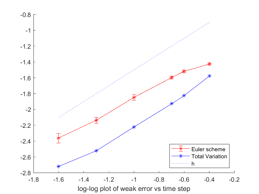
Figure 1: Example 1: mixture of two univariate Gaussian distributions (4.2). The global error and the total variation distance for the Euler method. Error bars indicate the Monte Carlo error.

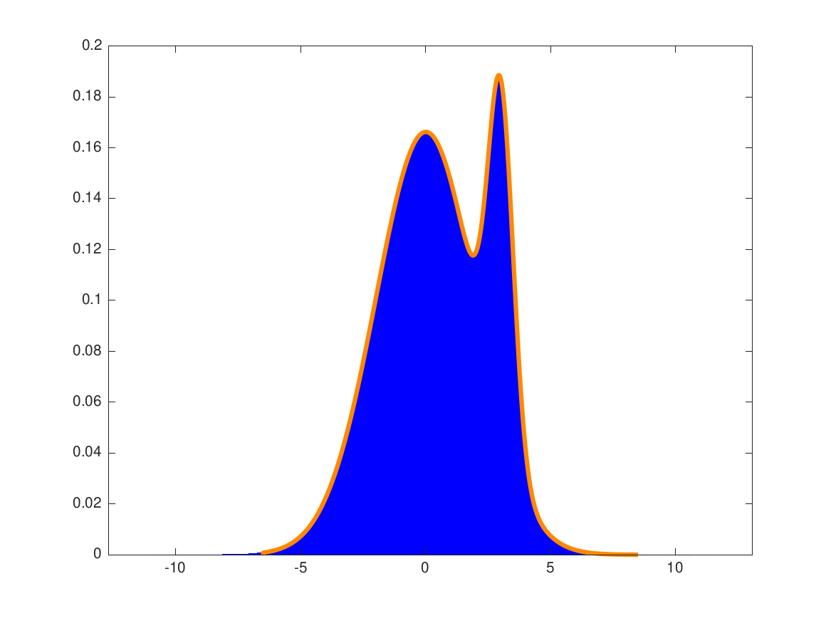
Figure 2: Example 1. Plot of the exact density $\rho(x)$ (4.2) (orange) and the normalized histogram corresponding to the Euler approximation (blue) with $h=0.025$, $T=100$ and $M=4\cdot 10^{8}$.

Example 2. Consider a mixture of two univariate Gaussian distributions and a distribution corresponding to a nonconvex potential $U(x;3)=\beta(x^{4}-4x^{2})$:

$$\rho(x)=\frac{1}{\mathcal{Z}}\left[\alpha_{1}\exp\left(-\frac{(x-\mathrm{m}_{1})^{2}}{2\sigma_{1}^{2}}\right)+\alpha_{2}\exp\left(-\frac{(x-\mathrm{m}_{2})^{2}}{2\sigma_{2}^{2}}\right)+\alpha_{3}\exp\left(-\beta(x^{4}-4x^{2})\right)\right],\ \ x\in\mathbb{R},$$ (4.3)

where $\mathcal{Z}$ is the normalisation constant. The parameters used are given in Table 3 and for test purposes we take $\varphi(x;m)=x^{2}.$ The exact value $\varphi^{erg}=6.98355$ $(5$ d.p.$).$ The results are given in Table 4 and Fig. 3 which show first order convergence in $h$ of the Euler method (3.10).

Table 3: Example 2. The parameters of the mixture (4.3).

$m$	$1$	$2$	$3$
$\alpha_{m}$	$0.8$	$1$	$0.4$
$c_{m}$	$3.5$	$-3$
$\sigma_{m}$	$1$	$0.6$
$\beta$			$0.25$

Table 4: Example 2: mixture distribution (4.3). The global error for the estimator $\hat{\varphi}$ of $\varphi^{erg}$ and the total variation.

$h$ $M$ $T$ $\hat{\varphi}^{erg}$ $\hat{\varphi}^{erg}-\varphi^{erg}$ $2\sqrt{\bar{D}_{M}/M}$ TVD $0.4$ $10^{7}$ $200$ $6.731$ $-0.253$ $0.013$ $0.096$ $0.25$ $10^{6}$ $200$ $6.816$ $-0.167$ $0.014$ $0.066$ $0.2$ $10^{6}$ $200$ $6.837$ $-0.146$ $0.014$ $0.054$ $0.1$ $10^{7}$ $200$ $6.9082$ $-0.0754$ $0.0043$ $0.025$ $0.05$ $10^{8}$ $200$ $6.9424$ $-0.0411$ $0.0014$ $0.012$ $0.025$ $10^{8}$ $200$ $6.9631$ $-0.0204$ $0.0014$ $0.0067$

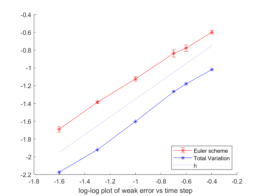
Figure 3: Example 2: mixture distribution (4.3). Global error and the total variation distance for the Euler method. Error bars indicate the Monte Carlo error.

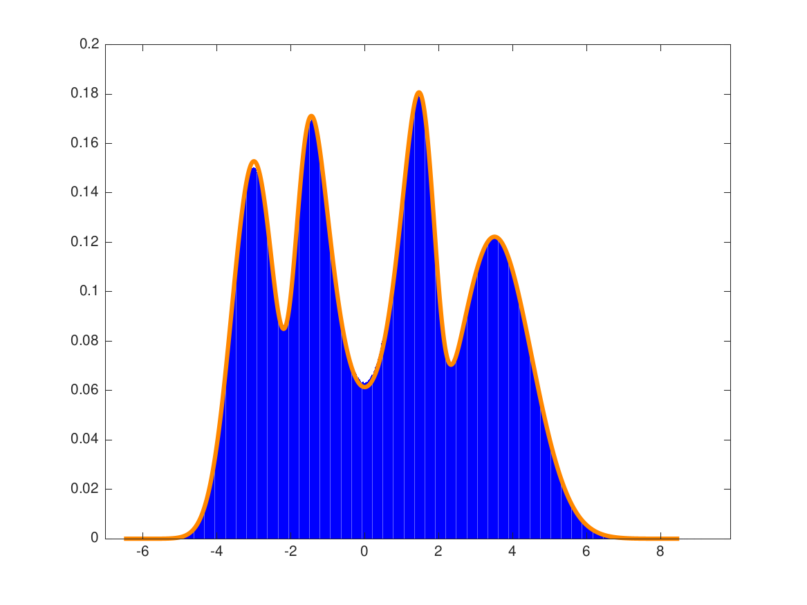
Figure 4: Example 2. Plot of the exact density $\rho(x)$ (4.3) (orange) and the normalized histogram corresponding to the Euler approximation (blue) with $h=0.025$, $T=200$ and $M=10^{8}$.

The gradient of the potential $U(x;3)$ is growing faster than linearly at infinity and hence Assumption 3.6 is not satisfied. As it is well known (see [15, 31, 22] and references therein), explicit Euler-type schemes are divergent when SDEs’ coefficients do not satisfy the global Lipschitz condition. The concept of rejecting exploding trajectories from [23, 24] allows us to apply any numerical method to SDEs with nonglobally Lipschitz coefficients for estimating averages $E\varphi(X(T))$. The concept is based on rejecting trajectories which leave a sufficiently large ball $S_{R}:=\{x:|x|<R\}$ during the time $T$ that contributes a very small additional error to the overall simulation error thanks to probability of $X(t),$ $t\in[0,T],$ being exponentially small [9, 23, 24, 22]. Here we implement this concept as follows: if $|X_{k}|\geq 100$ for any $k=1,\ldots,N,$ then we set $X_{n}=0$ for $n\geq k.$ For $h=0.4$ there were $3.5\%$ rejected trajectories, for $h=0.25$ there were just $3$ rejected trajectories out of $10^{6}$ and none for smaller time steps. The experimental results confirm that the concept of rejecting exploding trajectories can be successfully applied in the considered SDEwS setting.

Example 3. Consider a mixture of two multivariate Gaussian distributions:

$$\rho(x)=\frac{1}{\mathcal{Z}}\left[\alpha_{1}\exp\left(-\frac{1}{2}(x-\mathrm{m}_{1})^{\top}\Sigma_{1}^{-1}(x-\mathrm{m}_{1})\right)+\alpha_{2}\exp\left(-\frac{1}{2}(x-\mathrm{m}_{2})^{\top}\Sigma_{2}^{-1}(x-\mathrm{m}_{2})\right)\right],\ \ x\in\mathbb{R}^{2},$$ (4.4)

where $\mathcal{Z}$ is the normalisation constant, $\mathrm{m}_{i}$ are mean vectors, and $\Sigma_{i}$ are covariance matrices:

$$\Sigma_{i}=\left[\begin{array}[]{cc}\sigma_{1i}&r_{i}\\ r_{i}&\sigma_{2i}\end{array}\right].$$

The parameters used are given in Table 5 and for test purposes we take $\varphi(x;m)=|x|^{2}.$ The density $\rho(x)$ is plotted in Fig. 5.

Table 5: Example 3. The parameters of the mixture (4.4).

$i$	$1$	$2$
$\alpha_{i}$	$0.7$	$0.5$
$\mathrm{m}_{i}$	$(1,1)^{\top}$	$(-2,-1)^{\top}$
$\sigma_{1i}$	$2$	$1$
$\sigma_{2i}$	$0.5$	$1$
$r_{i}$	$0.1$	$-0.1$

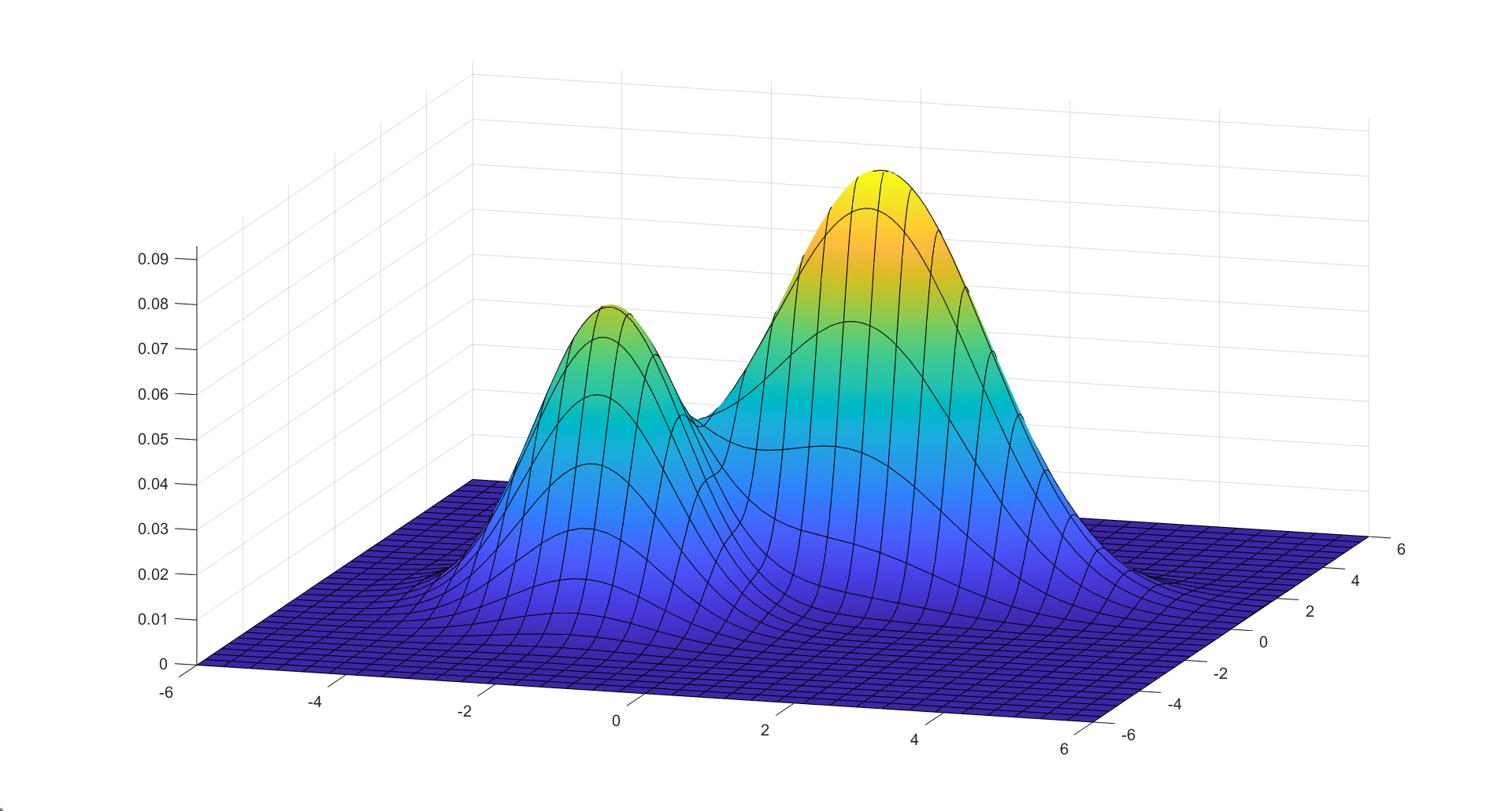
Figure 5: Example 3: mixture distribution $\rho$ from (4.4) with parameters as in Table 5.

The exact value $\varphi^{erg}=5.541667$ $(6$ d.p.$).$ The results of the experiments are presented in Table 6 and Fig. 6, which again show first order convergence in $h$ of the Euler method (3.10) as expected. Figure 7 gives the difference between the normalized histogram corresponding to the Euler approximation and the exact density $\rho(x)$ (4.4).

Table 6: Example 3: mixture of two univariate Gaussian distributions (4.2). The global error for the estimator $\hat{\varphi}$ of $\varphi^{erg}$ and the total variation.

$h$ $M$ $T$ $\hat{\varphi}^{erg}$ $\hat{\varphi}^{erg}-\varphi^{erg}$ $2\sqrt{\bar{D}_{M}/M}$ TVD $0.5$ $10^{6}$ $200$ $5.8559$ $0.3142$ $0.0101$ $0.0744$ $0.4$ $10^{6}$ $200$ $5.7798$ $0.2381$ $0.0099$ $0.0581$ $0.32$ $10^{7}$ $200$ $5.7279$ $0.1862$ $0.0031$ $0.0430$ $0.25$ $10^{8}$ $200$ $5.6808$ $0.1392$ $0.0010$ $0.0302$ $0.2$ $4\cdot 10^{8}$ $200$ $5.6528$ $0.1112$ $0.0005$ $0.0238$ $0.16$ $4\cdot 10^{8}$ $200$ $5.6292$ $0.0876$ $0.0005$ $0.0197$ $0.1$ $10^{9}$ $200$ $5.5961$ $0.0544$ $0.0003$ 0.0131

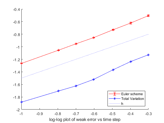
Figure 6: Example 3: mixture distribution (4.4). Global error and the total variation distance for the Euler method. Error bars indicate the Monte Carlo error.

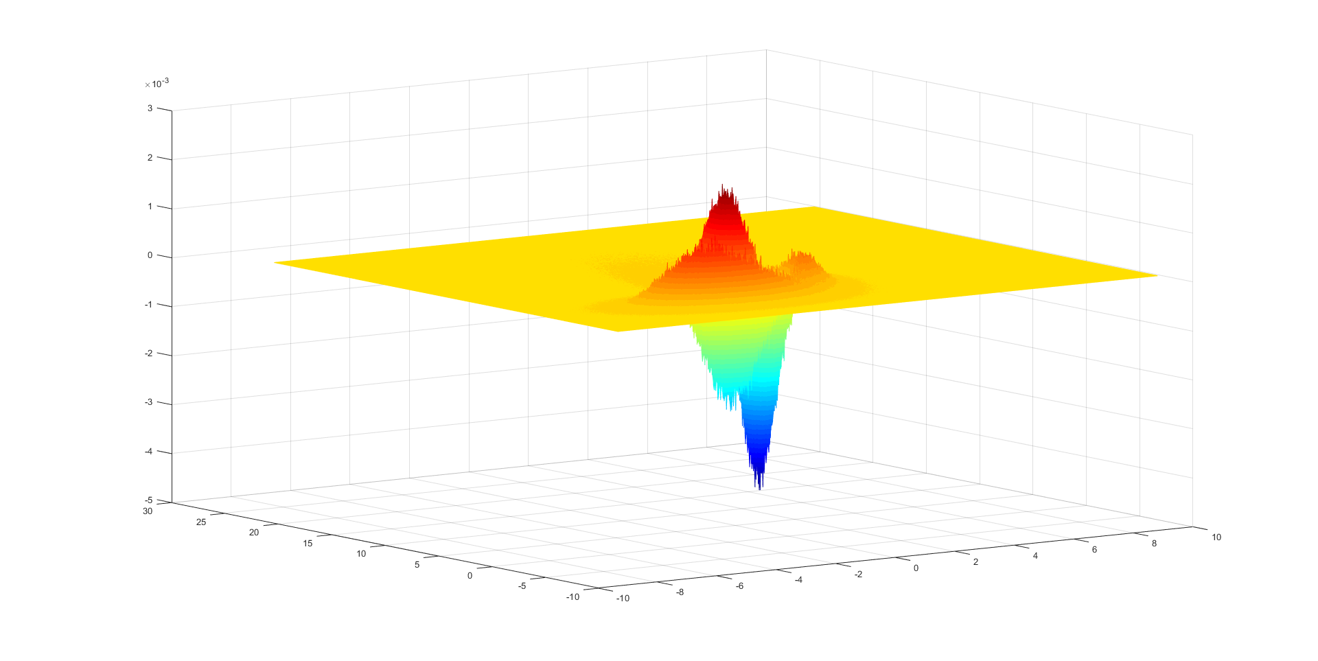
Figure 7: Example 3: The difference between the normalized histogram corresponding to the Euler approximation with $h=0.1$, $M=10^{9}$, $T=200$ and the exact density $\rho$ from (4.4) with parameters as in Table 5.

5 Proofs

The proofs of both Theorems 3.4 and 3.7 follow the same path: we first prove a second-order weak error bound for the corresponding one-step approximation (Lemmas 5.2 and 5.4) and then appropriately re-write the global error to sum up the local errors.

5.1 Finite-time convergence

The proof of the next lemma on boundedness of moments of the Euler scheme under weaker conditions than Assumption 3.3 can be found e.g. in [33, Lemma 3.1].

Lemma 5.1

Let Assumption 3.3 hold. Then the method (3.4) has finite moments, i.e., for all $p\geq 1:$

$$E\left(|X_{k}|^{2p}\right)\leq K(1+|x|^{2p}),$$

where $K>0$ does not depend on $h$ and $x.$

The following error gives the one-step error estimate.

Lemma 5.2

Let Assumption 3.3 hold. Then the one-step error of the method (3.4) is estimated as

$$\left|Eu(t+h,X_{1};\mu_{1})-u(t,x;m)\right|\leq C(1+|x|^{\varkappa})h^{2},$$

where $u(t+h,x,m),$ $m\in\mathcal{M},$ is a solution of (2.6), $C>0$ and $\varkappa\geq 1$ do not depend on $h,$ $x$ and $m.$

Proof. Using Taylor’s expansion, Assumption 3.3, (3.8), the estimate (3.3) and the backward Kolmogorov equation (2.6), we obtain

$$Eu(t+h,X_{1};\mu_{1})-u(t,x;m)$$

$$= h\sum_{j\neq m}q_{mj}(x)Eu(t+h,X_{1};j)+\left(1-hq_{m}(x)\right)Eu(t+h,X_{1};m)-u(t,x;m)$$

$$= h\sum_{j\neq m}q_{mj}(x)u(t,x;j)-hq_{m}(x)u(t,x;m)+Eu(t+h,X_{1};m)-u(t,x;m)+r_{1}(t,x)$$

$$= h\left[\frac{\partial}{\partial t}u(t,x;m)-\frac{1}{2}\nabla U(x,m)\cdot\nabla u(t,x;m)+\frac{1}{2}\Delta u(t,x;m)+\sum_{j\neq m}q_{mj}(x)u(t,x;j)-q_{m}(x)u(t,x;m)\right]$$

$$+r_{2}(t,x)=r_{2}(t,x),$$

where

$$|r_{i}(t,x)|\leq C(1+|x|^{\varkappa})h^{2}.$$

$\ \square\vskip 6.0pt plus 2.0pt minus 2.0pt$

Proof of Theorem 3.4. We re-write the global error using the Feynman-Kac formula (2.7):

$$\left|E\varphi(X_{N};\mu_{N})-E\varphi(X_{t,x,m}(T);\mu_{t,x,m}(T))\right|=\left|Eu(t_{N},X_{N};\mu_{N})-u(t,x;m)\right|$$

$$=\left|E\sum_{k=0}^{N-1}(u(t_{k+1},X_{k+1};\mu_{k+1})-u(t_{k},X_{k};\mu_{k}))\right|$$

$$=\left|\sum_{k=0}^{N-1}E\left(E\left[u(t_{k+1},X_{k+1};\mu_{k+1})-u(t_{k},X_{k};\mu_{k})|X_{k};\mu_{k}\right]\right)\right|$$

$$\leq\sum_{k=0}^{N-1}E\left|E\left[u(t_{k+1},X_{k+1};\mu_{k+1})-u(t_{k},X_{k};\mu_{k})|X_{k};\mu_{k}\right]\right|\leq Ch^{2}\sum_{k=0}^{N-1}E(1+|X_{k+1}|^{\varkappa})$$

$$\leq Ch(1+|x|^{\varkappa}),$$

where we applied Lemmas 5.1 and 5.2. $\ \square$

5.2 Ergodic limits convergence

We start with proving an estimate for the moments of the method (3.10).

Lemma 5.3

Let Assumption 2.1 hold. Then the method (3.10) has finite moments, i.e., for sufficiently small $h>0$ and all $p\geq 1:$

$$E\left(|X_{k}|^{2p}\right)\leq K(1+|x|^{2p}e^{-\lambda t_{k}}),$$

where $K>0$ does not depend on $h,$ $T$ and $x.$

Proof. We note that the constant $K>0$ is changing from line to line. We have

$$E|X_{k+1}|^{2p} = E|X_{k}|^{2p}+pE|X_{k}|^{2p-2}[2(X_{k}\cdot(X_{k+1}-X_{k}))+(2p-1)|X_{k+1}-X_{k}|^{2}]$$

$$+K\sum_{l=3}^{2p}E|X_{k}|^{2p-l}|X_{k+1}-X_{k}|^{l},$$

where $K>0$ depends on $p$ only. Using that $|\nabla U(x;m)|\leq K(1+|x|),$ (3.8) and (2.12), we obtain

$$E[X_{k}\cdot(X_{k+1}-X_{k})|X_{k},\mu_{k}] \leq -\frac{h}{2}X_{k}\cdot\nabla U(X_{k},\mu_{k})\leq-\frac{h}{2}c_{1}|X_{k}|^{2}+\frac{h}{2}c_{2},\,$$

$$E[|X_{k+1}-X_{k}|^{2}|X_{k},\mu_{k}] \leq Kh^{2}|X_{k}|^{2}+h,$$

$$E[|X_{k+1}-X_{k}|^{l}|X_{k},\mu_{k}] \leq Kh^{l}|X_{k}|^{l}+Kh^{l/2},\;l\geq 3,$$

with $K>0$ independent of $h$.

Then, using Young’s inequality (i.e., for $y,z\geq 0:$ $yz\leq\epsilon^{i}\frac{y^{i}}{i}+\epsilon^{-j}\frac{z^{j}}{j}$ with $\epsilon>0$, $i,j>1$ and $\frac{1}{i}+\frac{1}{j}=1)$, we get (where needed with a new $K>0$ independent of $h):$

$$2pE|X_{k}|^{2p-2}(X_{k}\cdot(X_{k+1}-X_{k}))\leq-pc_{1}hE|X_{k}|^{2p}+phKE|X_{k}|^{2p-2}$$

$$\leq-pc_{1}hE|X_{k}|^{2p}+(p-1)c_{1}h\mathbb{E}|X_{k}|^{2p}+hK^{p}\left(\frac{1}{c_{1}}\right)^{p-1}$$

$$=-c_{1}hE|X_{k}|^{2p}+hK^{p}\left(\frac{1}{c_{1}}\right)^{p-1},$$

$$p(2p-1)E|X_{k}|^{2p-2}|X_{k+1}-X_{k}|^{2}\leq p(2p-1)Kh^{2}|X_{k}|^{2p}+hp(2p-1)E|X_{k}|^{2p-2}$$

$$\leq Kh^{2}|X_{k}|^{2p}+\frac{c_{1}}{2}hE|X_{k}|^{2p}+\frac{[(2p-1)(p-1)]^{p}}{p-1}\left(\frac{2}{c_{1}}\right)^{p-1}h,$$

and for $l\geq 3$

$$E|X_{k}|^{2p-l}|X_{k+1}-X_{k}|^{l}\leq Kh^{l}|X_{k}|^{2p}+Kh^{l/2}E|X_{k}|^{2p-l}$$

$$\leq Kh^{l}|X_{k}|^{2p}+\frac{c_{1}h^{l/2}}{2p}\mathbb{E}|X_{k}|^{2p}+Kh^{l/2}$$

Thus

$$E|X_{k+1}|^{2p}\leq E|X_{k}|^{2p}-\frac{c_{1}}{2}h(1-\sqrt{h}-Kh)E|X_{k}|^{2p}+Kh,$$

whence by Gronwall’s lemma

$$E|X_{k+1}|^{2p}\leq\left(1-\frac{c_{1}h}{2}(1-\sqrt{h}-Kh)\right)^{k}|x|^{2p}+\frac{2K}{c_{1}(1-\sqrt{h}-Kh)}\left[1-\left(1-\frac{c_{1}h}{2}(1-\sqrt{h}-Kh)\right)^{k}\right].$$

$\ \square\vskip 6.0pt plus 2.0pt minus 2.0pt$

The local error of the method (3.10) is given in the next lemma.

Lemma 5.4

Let Assumption 3.6 hold. Then the one-step error of the method (3.10) is estimated as

$$\left|Eu(t+h,X_{1};\mu_{1})-u(t,x;m)\right|\leq C(1+|x|^{\varkappa})e^{-\lambda(T-t)}h^{2},$$

where $u(t+h,x,m),$ $m\in\mathcal{M},$ is a solution of (2.21), $C>0$ and $\varkappa\geq 1$ do not depend on $T$ and $h.$

Proof. Analogously to (5.1) but using (2.21), we have

$$Eu(t+h,X_{1};\mu_{1})-u(t,x;m)=r_{3}(t,x),$$

where the reminder $r_{3}(t,x)$ is a sum of terms containing derivatives of $u$ and the coefficients of the SDEwS (2.13), (2.14) and hence by (3.9)

$$\left|Er_{3}(t,x)\right|\leq C(1+|x|^{\varkappa})e^{-\lambda(T-t)}h^{2},$$

where $C>0\$is independent of $h,$ $t,$ $T$ and $x.$  $\square\vskip 6.0pt plus 2.0pt minus 2.0pt$

Proof of Theorem 3.7. Using (2.16) and Lemmas 5.4 and 5.3, we obtain

$$\left|E\varphi(X_{N};\mu_{N})-\varphi^{erg}\right|$$

$$\leq \left|E\varphi(X_{N};\mu_{N})-E\varphi(X_{0,x,m}(T);\mu_{0,x,m}(T))\right|+\left|E\varphi(X_{0,x,m}(T);\mu_{0,x,m}(T))-\varphi^{erg}\right|$$

$$\leq \sum_{k=0}^{N-1}E\left|E\left[u(t_{k+1},X_{k+1};\mu_{k+1})-u(t_{k},X_{k};\mu_{k})|X_{k};\mu_{k}\right]\right|+C\left(1+|x|^{\kappa}\right)e^{-\lambda T}$$

$$\leq Ch^{2}\sum_{k=0}^{N-1}e^{-\lambda(T-t_{k})}(1+E|X_{k}|^{\varkappa})+C\left(1+|x|^{\kappa}\right)e^{-\lambda T}\leq C\left[h+(1+|x|^{\kappa})\exp(-\lambda T)\right].$$

$\ \square\vskip 6.0pt plus 2.0pt minus 2.0pt$

Proof of Theorem 3.8. Thanks to (3.9), we get

$$\left|h\sum_{l=1}^{L}E\varphi(X_{0,x,m}(t_{l});\mu_{0,x,m}(t_{l}))-\int\limits_{0}^{\tilde{T}}E\varphi(X_{0,x,m}(s);\mu_{0,x,m}(s))ds\right|$$

$$= \left|h\sum_{l=1}^{L}u(0,x;m;t_{l})-\int\limits_{0}^{\tilde{T}}u(0,x;m;s)ds\right|=\left|h\sum_{l=1}^{L}u(-t_{l},x;m;0)-\int\limits_{0}^{\tilde{T}}u(-s,x;m;0)ds\right|$$

$$\leq Ch^{2}\sum_{l=1}^{L}\left(1+|x|^{\kappa}\right)e^{-\lambda(T-t_{l})}\leq Ch\left(1+|x|^{\kappa}\right).$$

Using Theorem 3.7, (5.2) and (3.17), we obtain

$$\left|E\check{\varphi}^{erg}-\varphi^{erg}\right| \leq \left|\frac{1}{L}\sum_{l=1}^{L}\left[E\varphi(X_{l};\mu_{l})-E\varphi(X_{0,x,m}(t_{l});\mu_{0,x,m}(t_{l}))\right]\right|$$

$$+\left|\frac{1}{L}\sum_{l=1}^{L}E\varphi(X_{0,x,m}(t_{l});\mu_{0,x,m}(t_{l}))-\frac{1}{\tilde{T}}E\int\limits_{0}^{\tilde{T}}\varphi(X_{0,x,m}(s);\mu_{0,x,m}(s))ds\right|$$

$$+\left|\frac{1}{\tilde{T}}E\int\limits_{0}^{\tilde{T}}\varphi(X_{0,x,m}(s);\mu_{0,x,m}(s))ds-\varphi^{erg}\right|$$

$$\leq \frac{1}{L}\sum_{l=1}^{L}C\left[h+(1+|x|^{\kappa})\exp(-\lambda t_{l})\right]+C\frac{h}{\tilde{T}}\left(1+|x|^{\kappa}\right)+C\left(1+|x|^{\kappa}\right)\frac{1}{\tilde{T}}$$

$$\leq C\left(h+\frac{1+|x|^{\kappa}}{\tilde{T}}\right).$$

$\square$

Remark 5.5

The following system of Poisson equations is associated with SDEwS (2.13), (2.14) with $Q(x)$ satisfying (2.18):

$$\mathcal{L}u(x;m)=\varphi(x;m)-\varphi_{m}^{erg},\ x\in\mathbb{R}^{d},\ m\in\mathcal{M},$$ (5.3)

where $\mathcal{L}$ is as in (2.21) and

$$\varphi_{m}^{erg}=\int_{\mathbb{R}^{d}}\varphi(x;m)\rho(x;m)dx$$

with $\rho(x;m)$ from (2.10). If $U(x,m)\in C^{3}(\mathbb{R}^{d}),$ $m\in\mathcal{M},$ and satisfy (2.12), and the elements $q_{ij}(x)$ of the matrix $Q(x)$ are positive functions bounded in $\mathbb{R}^{d}$ and belong to $C^{2}(\mathbb{R}^{d}),$ and the functions $\varphi(x;m),$ $m\in\mathcal{M},$ and their derivatives $\frac{\partial^{|j|}\varphi}{\partial x^{j_{1}}\cdots\partial x^{j_{d}}},$ $|j|\leq 2,$ are continuous and belong to the class $\mathbf{F,}$ then the solution to the system of elliptic PDEs (5.3) satisfies the following estimate for some $\kappa\geq 1$ [5]:

$$\sum\limits_{|j|=0}^{4}\left|\frac{\partial^{|j|}}{\partial x^{j_{1}},\dots,\partial x^{j_{d}}}u(t,x;m)\right|\leq K(1+|x|^{\kappa}),$$

where $K>0$ does not depend on $x$. The Poisson equation can potentially be used in proving properties of the time-averaging estimator $\check{\varphi}^{erg}$ analogously to [16] (see also [11, 2]).

References

- [1] J. Bao, J. Shao, C. Yuan. Approximation of invariant measures for regime-switching diffusions. Potential Analysis 44 (2016), 707–727.
- [2] K. Bharath, A. Lewis, A. Sharma, M.V. Tretyakov. Sampling and estimation on manifolds using the Langevin diffusion. arXiv:2312.14882, 2023.
- [3] N. Bouguila, W. Fan. Mixture models and applications. Springer, 2020.
- [4] B.S. Everitt, D.J. Hand. Finite mixture distributions. Springer, 1981.
- [5] A. Fridman. Partial differential equations of parabolic type. Prentice-Hall, 1964.
- [6] S. Fruehwirth-Schnatter. Finite mixture and Markov switching models. Springer, 2007.
- [7] Z. Gou, X. Tu, S.V. Lototsky, R. Ghanem. Switching diffusions for multiscale uncertainty quantification. Inter. J. Non-Linear Mechanics (2024), 104793.
- [8] M. Hutzenthaler and A. Jentzen. Numerical approximations of stochastic differential equations with non-globally Lipschitz continuous coefficients. Mem. Amer. Math. Soc., vol. 236. AMS, Providence, 2015.
- [9] R.Z. Khasminskii. Stochastic stability of differential equations. Springer, 2012.
- [10] O.A. Ladyzhenskaya, V.A. Solonnikov, N.N. Ural’ceva, Linear and quasilinear equations of parabolic type. Amer. Math. Soc., 1988.
- [11] B. Leimkuhler, A. Sharma, M. V. Tretyakov. Simplest random walk for approximating Robin boundary value problems and ergodic limits of reflected diffusions. Ann. Appl. Probab. 33 (2023), 1904–1960.
- [12] X. Li, Q. Ma, H. Yang, C. Yuan. The numerical invariant measure of stochastic differential equations with Markovian switching. SIAM J. Numer. Anal. 56 (2018), 1435–1455.
- [13] X. Mao, C. Yuan. Stochastic differential equations with Markovian switching. Imperial College Press, 2006.
- [14] X. Mao, C. Yuan, G. Yin. Numerical method for stationary distribution of stochastic differential equations with Markovian switching. J. Comp. Appl. Math. 174 (2005), 1–27.
- [15] J.C. Mattingly, A.M. Stuart, D.J. Higham. Ergodicity for SDEs and approximations: Locally Lipschitz vector fields and degenerate noise. Stoch. Proc. Appl., 101 (2002), 185–232.
- [16] J.C. Mattingly, A.M. Stuart, M.V. Tretyakov. Convergence of numerical time-averaging and stationary measures via Poisson equations. SIAM J. Numer. Anal. 48 (2010), 552–577.
- [17] H. Mei, G. Yin. Convergence and convergence rates for approximating ergodic means of functions of solutions to stochastic differential equations with Markov switching. Stoch. Proc. Appl. 125 (2015), 3104–3125.
- [18] G.N. Milstein. Interaction of Markov processes. Theory Prob. Appl. 17 (1972), 36–45.
- [19] G.N. Milstein. A method with second order accuracy for the integration of stochastic differential equations. Theor. Prob. Appl. 23 (1978), 414–419.
- [20] G.N. Milstein. Probabilistic solution of linear systems of elliptic and parabolic equations. Theor. Prob. Appl. 23 (1978), 851–855.
- [21] G.N. Milstein. Weak approximation of solutions of systems of stochastic differential equations. Theor. Prob. Appl. 30 (1985), 706–721.
- [22] G.N. Milstein, M.V. Tretyakov. Stochastic numerics for mathematical physics. 2nd edition. Springer, 2021.
- [23] G.N. Milstein, M.V. Tretyakov. Numerical integration of stochastic differential equations with nonglobally Lipschitz coefficients. SIAM J. Numer. Anal. 43 (2005), 1139–1154.
- [24] G.N. Milstein, M.V. Tretyakov. Computing ergodic limits for Langevin equations. Phys. D 229 (2007), 81–95.
- [25] G.O. Roberts, R.L. Tweedie. Exponential convergence of Langevin distributions and their discrete approximations. Bernoulli 2 (1996), 341–363.
- [26] A.V. Skorohod. Asymptotic methods in the theory of stochastic differential equations. AMS, 1989.
- [27] J. Shao. Invariant measures and Euler–Maruyama’s approximations of state-dependent regime-switching diffusions. SIAM J. Control Optim. 56 (2018), 3215–3238.
- [28] D. Talay. Discrétisation d’une équation différentielle stochastique et calcul approché d’espérances de fonctionnelles de la solution. Math. Model. Numer. Anal. (ESAIM) 20 (1986), 141–179.
- [29] D. Talay, L. Tubaro. Expansion of the global error for numerical schemes solving stochastic differential equations. Stoch. Anal. Appl. 8 (1990), 483–509.
- [30] D. Talay. Second-order discretization schemes for stochastic differential systems for the computation of the invariant law. Stoch. Stoch. Reports, 29 (1990), 13–36.
- [31] D. Talay. Stochastic Hamiltonian systems: exponential convergence to the invariant measure, and discretization by the implicit Euler scheme. Markov Proc. Relat. Fields, 8 (2002), 163–198.
- [32] M.V. Tretyakov, Z. Zhang. A fundamental mean-square convergence theorem for SDEs with locally Lipschitz coefficients and its applications. SIAM J. Numer. Anal. 51 (2013), 3135–3162.
- [33] G. Yin, X. Mao, C. Yuan, D. Cao. Approximation methods for hybrid diffusion systems with state-dependent switching processes: numerical algorithms and existence and uniqueness of solutions. SIAM J. Math. Anal. 41 (2010), 2335–2352.
- [34] G. Yin, C. Zhu. Hybrid switching diffusions: properties and applications. Springer, 2009.
- [35] G. Yin, C. Zhu. Properties of solutions of stochastic differential equations with continuous-state-dependent switching. J. Diff. Equations 249 (2010), 2409–2439.