Ultra-Low-Latency Edge Inference
for Distributed Sensing

Abstract

There is a broad consensus that artificial intelligence (AI) will be a defining component of the sixth-generation (6G) networks. As a specific instance, AI-empowered sensing will gather and process environmental perception data at the network edge, giving rise to integrated sensing and edge AI (ISEA). Many applications, such as autonomous driving and industrial manufacturing, are latency-sensitive and require end-to-end (E2E) performance guarantees under stringent deadlines. However, the 5G-style ultra-reliable and low-latency communication (URLLC) techniques designed with communication reliability and agnostic to the data may fall short in achieving the optimal E2E performance of perceptive wireless systems. In this work, we introduce an ultra-low-latency (ultra-LoLa) inference framework for perceptive networks that facilitates the analysis of the E2E sensing accuracy in distributed sensing by jointly considering communication reliability and inference accuracy. By characterizing the tradeoff between packet length and the number of sensing observations, we derive an efficient optimization procedure that closely approximates the optimal tradeoff. We validate the accuracy of the proposed method through experimental results, and show that the proposed ultra-Lola inference framework outperforms conventional reliability-oriented protocols with respect to sensing performance under a latency constraint.

I Introduction

Two of the main novelties expected in the upcoming sixth-generation (6G) of mobile networks are edge artificial intelligence (AI) and distributed sensing [1]. The former will feature ubiquitous deployment of AI and learning algorithms at the network edge to automate mobile applications [2, 3], whereas distributed sensing will facilitate large-scale sensor networks with, e.g., environment perception and localization capabilities [4]. The natural convergence of edge AI and distributed sensing, termed integrated sensing and edge AI (ISEA), will provide a platform that promises to revolutionize numerous Internet-of-Things domains, such as auto-driving, health-care, smart cities, and industrial manufacturing [5]. However, aligning ISEA with the ambitious 6G goals for achieving unprecedented end-to-end (E2E) low-latency, reliability, and mobility requires new breakthroughs in ISEA technologies. One representative application scenario is the Level 4/5 autonomy in autonomous driving that requires real-time object detection within 30 milliseconds and with an accuracy close to 100% [6]. As a step towards addressing this problem, we present the novel framework of ultra-low-latency (ultra-LoLa) Inference for ISEA, which enables ultra-LoLa short-packet transmission (SPT) of features extracted from remote sensing data. By carefully optimizing the tradeoff between communication reliability and sensing quality, the framework maximizes the E2E sensing accuracy given a stringent task completion deadline.

The development of ultra-LoLa transmission techniques accelerated in 5G where ultra-reliable and low latency communications (URLLC) was defined as one of 5G missions to support machine-to-machine applications [7]. Relevant techniques aim at realizing E2E latencies below one millisecond and packet-error rates of $10^{-5}$ or lower, allowing mission-critical applications (e.g., industrial automation) to be deployed in 5G networks. A main challenge confronting URLLC is to balance the tradeoffs among data rate, latency, and reliability. The short packets (or blocklengths) imposed by the strict deadline introduce a non-negligible transmission error probability, which depends on the operating regime [7]. When the channel diversity is limited and the transmitter only has statistical channel information, the reliability is dominated by deep fades and can be accurately characterized by outage expressions for infinite-length packets. On the other hand, when the transmitter has channel information or can leverage channel diversity, which is the focus in this paper, the reliability is mainly due to noise-induced decoding errors in the receiver. The resulting tradeoffs between packet error rate, data rate, and code length is a classic topic studied by information theorists [8]. Guided by these results, one approach that 5G engineers have adopted to implement URLLC is using SPT [9]. This comes at the cost of low data rates, which limits the applications of URLLC to those with relatively low-rate transmissions, e.g., transmission of commands to remote robots or data uploading by primitive sensors (e.g., humidity, temperature, or pollution) [10, 11]. Nevertheless, researchers have made diversified attempts to alleviate the limitation by designing customized SPT techniques including non-coherent transmission [12], optimal framework structures [13], power control [14], wireless power transfer [15], and multi-access schemes [10].

However, the existing SPT approaches targeting URLLC are insufficient to meet the requirements for ISEA. This is because ISEA applications are relatively data-intensive and frequently requires the transmission of high-dimensional features, resulting in a communication bottleneck caused by the SPT’s small payload sizes. The issue is exacerbated for tasks with stringent latency requirements, such as real-time object recognition for autonomous driving. Moreover, the E2E performance of sensing tasks (e.g., inference accuracy) cannot be accurately quantified by decoding error probability, which is more suitable for communication reliability assessment. While existing URLLC techniques designed for 5G focus a ultra high packet-level reliability, the target of ISEA is to achieve maximum E2E accuracy under a deadline constraint. Hence, two challenges faced by the deployment of ISEA in the 6G systems are: (i) overcoming the communication bottleneck with high rate, low latency feature uploading from distributed sensors; (ii) designing new SPT techniques based on E2E sensing performance metrics.

The proposed ultra-LoLa inference framework is based on the popular ISEA architecture, known as the multi-view convolutional neural network (MVCNN), provisioned with wireless connections between distributed sensors and an edge server [16]. The sensors employ lightweight pre-trained neural networks to extract features from their locally gathered data, which are then sent to the server for aggregation and inference through a deep neural network model. Diverse strategies have been proposed to tackle the communication bottleneck and enhance the E2E sensing performance. The majority of existing works consider a simplified point-to-point system with a single sensor/transmitter, for which MVCNN reduces to an architecture known as split inference that divides a global model into two parts for on-device feature extraction and on-server inference. In this scenario, the optimal model splitting point can be adjusted according to bandwidth and latency constraints [17], and the feature transmission can possibly be designed using joint source-channel coding (JSCC) to additionally cope with channel noise [18]. The communication overhead in ISEA can be further reduced via feature pruning and quantization [19], and task-relevant sensor scheduling [20]. Researchers have also studied the latency-accuracy tradeoffs in other ISEA strategies, such as parallel processing and early exiting [21], and found ways to balance the computational cost and the communication overhead [19]. From the perspective of multi-access for ISEA, researchers have constructed a class of simultaneous-access schemes, called over-the-air computing (AirComp), to be a promising solution for realizing over-the-air feature aggregation when there are many sensors [22, 23]. Recent work has also explored the E2E design integrating radar, sensing, communication, and AirComp [24]. However, while AirComp brings many advantages, its uncoded analog transmission can expose data to interference and noise, and encounters the issue of compatibility with existing digital systems. Overall, the existing wireless techniques for ISEA are based on the assumption of long-packet transmission, which is not valid in the ultra-LoLa regime required for ultra-LoLa ISEA, which motivates the current work.

In this work, we propose an ultra-LoLa inference framework designed for SPT to achieve the optimal E2E performance of ISEA systems, i.e., maximizing the sensing accuracy referring to the accuracy of inference on uploaded data features. We consider an ultra-LoLa application with a stringent deadline (e.g., 1ms for 6G) such that SPT is needed. Underpinning the proposed framework is an important tradeoff, as revealed in this work, that exists between packet length and number of views. Specifically, longer packets ensure more reliable communication but result in a lower sensing accuracy due to fewer sensor views that can be uploaded before the deadline. This reliability-view tradeoff necessitates the optimization of packet length to maximize the E2E sensing accuracy. In particular, focusing only on reliability, as in traditional URLLC, results in a sub-optimal sensing performance.

We consider two sensing scenarios. The first is multi-snapshot sensing, where a single sensor captures a sequence of observations, such as images of a moving object, extracts features from each observation using a local pre-trained model. The features are then fused locally before being uploaded using point-to-point SPT to the server for inference. The other is multi-view sensing, where multiple sensors simultaneously capture different observations of the same object and upload their features over a multi-access channel to the edge server, which aggregates the features and performs joint inference. We study the problem under the assumption that the feature distribution follows a Gaussian mixture model (GMM), as widely used in machine learning (see, e.g., [25, 26]). With channel state information (CSI) at the transmitter, channel inversion is leveraged to ensure a fixed signal-to-noise ratio (SNR) for SPT. This is practical frame-based cellular system, as it offers data containers of deterministic length, which is important for scheduling in multi-user scenarios. Based on finite-blocklength information theory, we quantify the E2E sensing accuracy by the probability of correct classification of sensing objects, taking into account both sensing noise and transmission errors.

The key contributions and findings of our work are summarized as follows:

• E2E performance analysis: Tractable E2E performance analysis of ISEA is known to be challenging. Relevant results do not exist for ISEA with SPT, i.e., ultra-LoLa inference. To tackle the challenge, we adopt the popular GMM as feature distribution and derive a tight lower bound on classification accuracy as a function of the number of object classes and the minimum pairwise discriminant gain. The bound is a function of the feature size per sensor view and the number of views. A communication-computation integrated approach is then adopted to combine the preceding result with finite-blocklength information theory [8]. As a result, tractable expressions for E2E sensing accuracy are derived for both multi-snapshot and multi-view sensing under a task-deadline constraint, revealing the inherent reliability-view tradeoff discussed earlier and confirming the importance of packet-length optimization.

• Packet-length optimization: To facilitate E2E optimization, accurate surrogate functions are derived for the sensing accuracy, for both sensing scenarios under consideration. For multi-snapshot sensing, the surrogate is a log-concave function of the product of successful transmission probability and classification accuracy. For multi-view sensing, the derived surrogate function depends on the expected number of successfully transmitted views within the deadline. The unimodality of the surrogate functions allows the problem of accuracy maximization under a deadline constraint to be solved efficiently. The resulting optimal packet length reflects the influence of the SNR, sensing complexity (i.e., number of classes), and additional network parameters.

• Experiments: The analytical results are validated in ISEA experiments using both synthetic (i.e., GMM) and real datasets (i.e., ModelNet [16]). The proposed ultra-Lola inference designs are shown to achieve new-optimal performance and furthermore outperform traditional reliability-centered URLLC techniques.

The remainder of the paper is organized as follows. Sensing, communication, and inference models are defined in Section II. The E2E performance analysis for ultra-LoLa inference is presented in Section III, followed by a discussion on the optimal packet length in Section IV. Experimental results are given in Section V, and the paper is concluded in Section VI.

II Models and Metrics

The considered ultra-LoLa edge inference system consists of a single edge server performing remote object classification using $K$ distributed sensors. Time is divided into recurring inference rounds initiated by the edge server. In each round, the edge server requests the uploading of observations from sensors, which are assumed to capture the same object under different conditions (e.g., different angles and lighting conditions in the case of images). The uploaded observations are used for joint inference to recognize the associated object.

II-A Data and Inference Models

Each of the sensors produces an observation of a common object class $\ell$, and feeds it to a local pre-trained model to generate a corresponding feature vector, $\mathbf{x}_{k}\in\mathbb{R}^{N}$. The feature vectors are assumed to be randomly drawn from a joint conditional distribution $(\mathbf{x}_{1},\ldots,\mathbf{x}_{K})\sim p_{\mathbf{x}_{1:K}}(\mathbf{x}_{1},\ldots,\mathbf{x}_{K}|\ell)$, and the common object class $\ell$ is assumed to be drawn uniformly from a set of $L$ classes, so that the joint feature distribution can be written as

$$(\mathbf{x}_{1},\ldots,\mathbf{x}_{K})\sim\frac{1}{L}\sum_{\ell=1}^{L}p_{\mathbf{x}_{1:K}}(\mathbf{x}_{1},\ldots,\mathbf{x}_{K}|\ell).$$ (1)

The distribution is next elaborated for two classifier models.

II-A1 Gaussian Mixture Model for Linear Classification

For tractability, the subsequent analysis focuses on the case where the feature vectors are drawn from a GMM [26, 27]. Specifically, we assume that each feature vector $\mathbf{x}_{k}$ is drawn independently from a Gaussian distribution with mean $\boldsymbol{\mu}_{\ell}\in\mathbb{R}^{N}$ and covariance matrix $\mathbf{C}\in\mathbb{R}^{N\times N}$. Note that the mean (or class centroid) depends on the class while the covariance matrix is assumed to be the same for all classes. Without loss of generality, we assume that $\mathbf{C}=\operatorname{diag}(C_{1,1},C_{2,2},\ldots,C_{N,N})$ is diagonalized, e.g., using singular value decomposition. The joint distribution in (1) becomes

$$(\mathbf{x}_{1},\ldots,\mathbf{x}_{K})\sim\frac{1}{L}\sum_{\ell=1}^{L}\prod_{k=1}^{K}\mathcal{N}\left(\mathbf{x}_{k}\mid\boldsymbol{\mu}_{\ell},\mathbf{C}\right),$$ (2)

where $\mathcal{N}\left(\mathbf{x}_{k}\mid\boldsymbol{\mu}_{\ell},\mathbf{C}\right)$ denotes the Gaussian probability density function (PDF) with mean $\boldsymbol{\mu}_{\ell}$ and covariance matrix $\mathbf{C}$. Finally, to characterize the discernibility between any pair of classes $\ell$ and $\ell^{\prime}$ of the GMM, we define the discriminant gain as the symmetric Kullback-Leibler (KL) divergence [27]:

$$\small\begin{split}g_{\ell,{\ell^{\prime}}}&=\sf{KL}(\mathcal{N}(\boldsymbol{\mu}_{\ell},\mathbf{C})\,||\,\mathcal{N}(\boldsymbol{\mu}_{\ell^{\prime}},\mathbf{C}))+\sf{KL}(\mathcal{N}(\boldsymbol{\mu}_{\ell^{\prime}},\mathbf{C})\,||\,\mathcal{N}(\boldsymbol{\mu}_{\ell},\mathbf{C}))\\ &=(\boldsymbol{\mu}_{\ell}-\boldsymbol{\mu}_{\ell^{\prime}})^{\sf{T}}\mathbf{C}^{-1}(\boldsymbol{\mu}_{\ell}-\boldsymbol{\mu}_{\ell^{\prime}}).\end{split}$$ (3)

We consider a maximum likelihood (ML) classifier for the distribution in (2), which relies on a classification boundary between a class pair being a hyperplane in the feature space. Due to the uniform prior on the object classes, the ML classifier is equivalent to a maximum a posteriori (MAP) classifier, and the estimated label $\hat{\ell}$ is obtained as

$$\begin{split}\hat{\ell}&=\operatorname*{argmax}_{\ell}\log\Pr(\overline{\mathbf{x}}|\ell)\\ &=\operatorname*{argmin}_{\ell}z_{\ell}(\overline{\mathbf{x}}),\end{split}$$ (4)

where $z_{\ell}(\overline{\mathbf{x}})=(\overline{\mathbf{x}}-\boldsymbol{\mu}_{\ell})^{\sf{T}}\mathbf{C}^{-1}(\overline{\mathbf{x}}-\boldsymbol{\mu}_{\ell})$ is the squared Mahalanobis distance between the input feature vector $\overline{\mathbf{x}}$ and the class centroid $\boldsymbol{\mu}_{\ell}$.

II-A2 General Model for CNN Classification

We also consider a more realistic but analytically intractable scenario in experiments, where feature vectors are extracted from images using a CNN, as shown in Fig. 1(c). The neural network model comprises multiple convolutional layers followed by multiple fully connected layers and a softmax output activation function that outputs a confidence score of each label. The layers are split into a sensor sub-model and a server sub-model, represented as functions $f_{\sf sen}(\cdot)$ and $f_{\sf ser}(\cdot)$, respectively. The feature vector is constructed by passing an image ${\mathbf{M}_{k}}$ of the common object through a pre-trained CNN, i.e., $\mathbf{x}_{k}=f_{\sf sen}(\mathbf{M_{k}})$. The feature vectors are then aggregated to $\overline{\mathbf{x}}$, and the confidence score of the server-side classifier can be obtained by feeding the aggregated feature vector into the server sub-model, i.e., $\{s_{1},\dots,s_{\ell},\dots,s_{L}\}=f_{\sf ser}\left(\overline{\mathbf{x}}\right)$. With such processing, the MVCNN classifier outputs the inferred label that has the maximum confidence score, i.e., $\hat{\ell}=\operatorname*{argmax}_{\ell}s_{\ell}$.

II-B Sensing Models

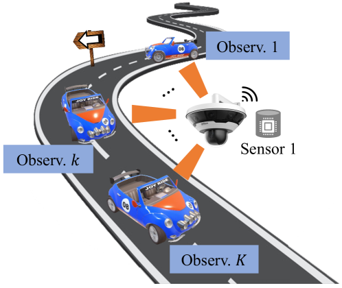
(a) Multi-snapshot sensing

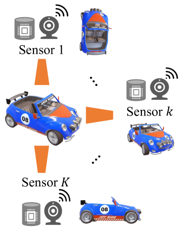
(b) Multi-view sensing

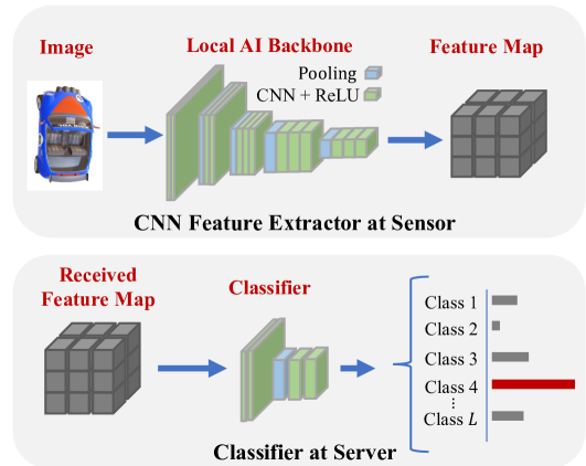
(c) CNN classifier

Figure 1: Sensing models and CNN classifier in an ultra-LoLa edge inference system.

Two sensing scenarios as illustrated in Fig. 1 are modeled as follows.

II-B1 Multi-Snapshot Sensing

As illustrated in Fig. 1(a), the $K$ observations are generated sequentially and then fused by a single device before being transmitted to the edge server. Multi-snapshot sensing represents, for instance, a scenario where the device captures a series of images of a moving object, e.g., a vehicle in an intelligent traffic monitoring system. We assume a sensing duration of $\Delta_{S}$ seconds, so that it takes a total of $T_{\sf{S}}=K\Delta_{S}$ seconds to generate the $K$ observations. The observations are then fused to an averaged feature vector $\overline{\mathbf{x}}\in\mathbb{R}^{N}$, given as

$$\overline{\mathbf{x}}=\frac{1}{K}\sum_{k=1}^{K}\mathbf{x}_{k},$$ (5)

which is transmitted to the edge server for inference.

II-B2 Multi-View Sensing

Compared to multi-snapshot sensing by a single sensor, multi-view sensing is distributed where the $K$ observations are produced and transmitted in parallel by $K$ sensors, as shown in Fig. 1(b). The total sensing duration is then simply $T_{\sf{S}}=\Delta_{S}$, and the edge server performs both feature fusion of the received feature vectors and inference.

II-C Short-Packet Transmission Model

The feature vector at each sensor device is uploaded to the edge server over a wireless channel with a total bandwidth of $B_{W}$ Hz. Each feature vector is quantized to a sufficiently large number of bits $NQ_{B}$, such that the quantization error is negligible. The quantized features are then encoded using a channel code and transmitted over $D$ complex channel uses (i.e., $D$ is the packet length and $NQ_{B}/D$ is the rate).

We assume random i.i.d. block-fading channels between the devices and the server, where the channel coefficient of device $k$ is $h_{k}$. The coefficient remains constant throughout the transmission of each feature vector. We assume that the devices have perfect knowledge of their channel coefficients via channel training, so that they can perform truncated channel inversion power control that is optimal in the finite blocklength regime [29]. On the other hand, the server learns about the channels only after receiving the feature vector transmissions in the uplink, and thus cannot perform scheduling based on channel information. Following the principle of truncated channel inversion, device $k$ inverts its channel only if its channel gain $|h_{k}|^{2}$ exceeds a threshold $G_{th}$, and otherwise stays silent by setting its transmission power to zero. We assume orthogonal transmissions such that the signal received by the server from device $k$ can be written as

$$\mathbf{y}_{k}=p_{k}h_{k}\mathbf{s}_{k}+\mathbf{w}_{k},$$ (6)

where $\mathbf{s}_{k}\in\mathbb{C}^{D}$ is the transmitted signal satisfying $(1/D)\|\mathbf{s}_{k}\|_{2}^{2}\leq 1$, $\mathbf{W}_{k}\sim\mathcal{CN}(0,B_{W}N_{0})$ is additive white Gaussian noise (AWGN) with noise spectral density $N_{0}$, and $p_{k}$ is the precoding coefficient given as

$$p_{k}=\begin{cases}\frac{\sqrt{P_{0}}h_{k}^{*}}{|h_{k}|^{2}},&|h_{k}|^{2}\geq G_{th},\\ 0,&|h_{k}|^{2}<G_{th},\end{cases}$$ (7)

where $P_{0}$ is the target signal power at the receiver. The activation probability, denoted by $\xi_{a}$, is then obtained as

$$\xi_{a}=\Pr(|h_{k}|^{2}\geq G_{th}).$$ (8)

We denote the subset of transmitting devices by $\mathcal{K}=\{k\in\{1,2,\ldots,K\}\mid|h_{k}|^{2}\geq G_{th}\}$. The threshold $G_{th}$ is chosen such that $\mathbb{E}[|p_{k}|^{2}]=\xi_{a}\mathbb{E}[|h_{k}|^{-2}]\leq P_{\max}$, where $P_{\max}$ is the long-term power constraint of the distributed sensing system.

Under the above assumptions, whenever the channel gain exceeds $G_{th}$, the channel is effectively an additive white Gaussian noise (AWGN) channel with SNR $\gamma=\frac{P_{0}}{N_{0}B_{W}}$ [29]. In this regime, the decoding error probability for a transmitting device ($k\in\mathcal{K}$) can be closely approximated as [8]

$$\varepsilon=Q\left(\ln(2)\sqrt{\frac{D}{V}}\left(\log_{2}(1+\gamma)-\frac{NQ_{B}}{D}\right)\right),$$ (9)

where $Q(x)=\frac{1}{\sqrt{2\pi}}\int_{x}^{\infty}e^{-\frac{t^{2}}{2}}dt$ and $V=1-(1+\gamma)^{-2}$ is the channel dispersion. Combining this with the probability of outage (when $|h_{k}|^{2}<G_{th}$), the probability of successful transmission, denoted as $\rho$, can be expressed as

$$\rho=\xi_{a}(1-\varepsilon).$$ (10)

We define $\hat{\mathcal{K}}\subseteq\mathcal{K}$ as the set of sensors that successfully transmit their feature vector.

II-D System Configurations and Multi-Access

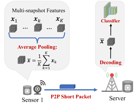
(a) Multi-snapshot sensing with point-to-point transmission

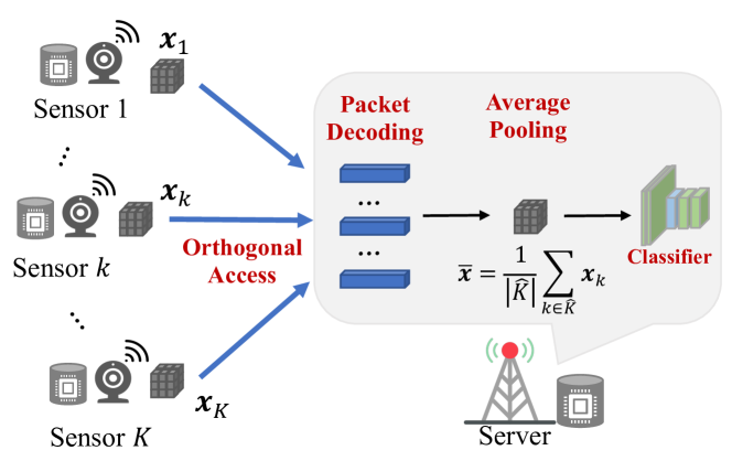
(b) Multi-view sensing with orthogonal access

Figure 2: Diagrams of multi-access models of the considered sensing tasks.

II-D1 Multi-Snapshot Sensing with Point-to-Point Transmission

For multi-snapshot sensing, the quantized fused feature vector $\overline{\mathbf{x}}$ in (5) is uploaded using the full system bandwidth $B_{W}$, as shown in Fig. 2(a). The transmission latency is then $T_{\sf{T}}=\frac{D}{B_{W}}$, where $D$ is the number of complex channel symbols. Upon successful transmission, the fused feature vector is used for inference at the edge server.

II-D2 Multi-View Sensing with Orthogonal Access

In multi-view sensing, we consider time division multiple access (TDMA) for feature uploading, as shown in Fig. 2(b). Specifically, the transmission of the packets is divided equally into $K$ time slots, each of which has access to the full bandwidth of $B_{W}$. Given the orthogonal transmission, each packet is decoded independently by the server with error probability $\varepsilon$ defined in (9). However, compared to the multi-snapshot setting the resulting transmission latency is $T_{\sf{T}}=\frac{DK}{B_{W}}$. After the transmissions, the server performs average pooling over all successfully received feature vectors, i.e., it computes the averaged feature vector

$$\overline{\mathbf{x}}=\frac{1}{\hat{|\mathcal{K}|}}\sum_{k\in\hat{\mathcal{K}}}\mathbf{x}_{k},$$ (11)

which is then fed into the classifier for inference.

II-E E2E Performance Metric

We measure the E2E performance by sensing accuracy. The metric is defined as the probability of correct classification by taking into account both the random observations and the transmission process. Specifically, for a given number of snapshots $K$, the sensing accuracy in the multi-snapshot setting, denoted as $\overline{E}_{\sf{ms}}$, is defined as

$$\overline{E}_{\sf{ms}}=\frac{\rho}{L}\sum_{\ell=1}^{L}\Pr(\hat{\ell}=\ell|\ell,K)+\frac{1-\rho}{L},$$ (12)

where $\Pr(\hat{\ell}=\ell|\ell,K)$ refers to the probability of correct classification with $K$ observations given the ground-truth label $\ell$. Note that the factor $\frac{1}{L}$ represents the inference accuracy of random guessing in the case of a transmission error. Similarly, in multi-view sensing, the sensing accuracy, denoted as $\overline{E}_{\sf{mv}}$, is given by

$$\begin{split}\overline{E}_{\sf{mv}}=\frac{1}{L}\sum_{\ell=1}^{L}\mathbb{E}_{|\hat{\mathcal{K}}|}\left[\Pr(\hat{\ell}=\ell|\ell,|\hat{\mathcal{K}}|)\mid\ell,K\right],\end{split}$$ (13)

where the expectation is over the number of received feature vectors $|\hat{\mathcal{K}}|$, taking into account that some of the $K$ users may fail to transmit their feature vectors.

III E2E Accuracy Analysis for Ultra-LoLa Inference

In this section, we analyze the sensing accuracy of ultra-LoLa edge inference for the two considered sensing scenarios. We consider an E2E deadline so that the sensing and transmission must be completed within a duration of $T$ seconds (in the order of a few milliseconds). Specifically, given sensing time $T_{\sf{S}}$ and transmission time $T_{\sf{T}}$, we require $T_{\sf{S}}+T_{\sf{T}}\leq T$.

III-A Sensing Accuracy for Multi-Snapshot Sensing

The computation of sensing accuracy in (12) relies on the explicit expression of classification accuracy with a given number of observations $K$, i.e., $\frac{1}{L}\sum_{\ell=1}^{L}\Pr(\hat{\ell}=\ell|\ell,K)$. However, it is difficult to obtain its closed-form expression due to the coupling among pairwise decision boundaries in a multi-class classifier. Instead, for a tractable analysis, we study the classification accuracy through the bound in Lemma 1.

Lemma 1 (Lower Bound on Classification Accuracy).

Conditioned on successful transmission and number of classes $L\geq 2$, the classification accuracy with $K$ snapshots, denoted as $A$, is lower bounded as

$$\small A =\frac{1}{L}\sum_{\ell=1}^{L}\Pr(\hat{\ell}=\ell|\ell,K)$$ (14)

$$\geq\left[1-(L-1)Q\left(\frac{\sqrt{Kg_{\min}}}{2}\right)\right]_{(1/L)^{+}},$$ (15)

where $[x]_{(1/L)^{+}}=\max\{1/L,x\}$ ensures an accuracy larger than random guessing probability $\frac{1}{L}$ and $g_{\min}=\min\{g_{\ell,\ell^{\prime}}|\ell,\ell^{\prime}\in\{1,2,\dots,L\},\ell\neq\ell^{\prime}\}$ is the minimum pairwise discrimination gain among all classes.

The proof is given in Appendix A.

Remark 1 (Classification Accuracy of Binary Classifier).

For a binary classifier with $L=2$, the classification accuracy in (15) reduces to the exact expression

$$A=Q\left(-\frac{\sqrt{Kg_{1,2}}}{2}\right),$$ (16)

where $g_{1,2}=\sum_{n=1}^{N}\frac{(\boldsymbol{\mu}_{1}(n)-\boldsymbol{\mu}_{2}(n))^{2}}{C_{n,n}}$ is the discrimination gain.

As observed in Lemma 1 and also (16), the lower bound on classification accuracy increases with the minimum discrimination gain and decreases with an increasing number of classes. These two factors determine the difficulty of the classification task.

For a given packet length $D$, the maximum accuracy is obtained when the number of observations $K$ is maximized while satisfying the task deadline $T$. Considering the constraint $T_{\sf{S}}+T_{\sf{T}}\leq T$ where $T_{\sf{S}}=K\Delta_{S}$, this quantity is given as

$$K_{\sf{ms}}=\left\lfloor\frac{T}{\Delta_{S}}-\frac{D}{B_{W}\Delta_{S}}\right\rfloor.$$ (17)

Substituting (15) and (17) into (12), the achievable sensing accuracy for multi-snapshot sensing is lower bounded in Proposition 1.

Proposition 1 (Sensing Accuracy for Multi-snapshot Sensing).

For a given packet length $D$, the achievable sensing accuracy for multi-snapshot sensing with task completion deadline $T$ can be lower bounded as

$$\begin{split}\overline{E}_{\sf{ms}}&\geq(L-1)\rho\left[\frac{1}{L}-Q\left(\frac{\sqrt{K_{\sf{ms}}g_{\min}}}{2}\right)\right]_{(1/L)^{+}}+\frac{1}{L},\end{split}$$ (18)

where $[x]_{(1/L)^{+}}=\max\{1/L,x\}$, $\rho$ is the successful transmission probability given in (10), and $K_{\sf{ms}}$ is given in (17).

Remark 2 (Reliability-View Tradeoff).

The lower bound on sensing accuracy in Proposition 1 highlights the tradeoff between communication reliability and the number of views. In particular, increasing the packet length $D$ increases the successful decoding probability, which in turn results in a higher successful transmission probability $\rho$, and vice versa. However, a large packet length comes at the cost of a smaller number of observations during the sensing phase, which decreases the discrimination gain $K_{\sf{ms}}G_{\min}$, and reduces the sensing accuracy due to increased sensing noise. Considering this tradeoff, the packet length $D$ should be optimized to maximize the sensing accuracy, which we do in Section IV.

III-B Sensing Accuracy for Multi-View Sensing

Next, we investigate the reliability-view tradeoff for multi-view sensing by applying the lower bound on classification accuracy from Lemma 1 to the multi-view sensing accuracy in (13). Since each view is transmitted independently, the sensing accuracy for multi-view sensing, denoted as $\overline{E}_{\sf{mv}}$, can be lower bounded as

$$\begin{split}\footnotesize\overline{E}_{\sf{mv}}&\geq\hat{E}_{\sf{mv}}\\ &=\sum_{|\hat{\mathcal{K}}|=0}^{K}P_{|\hat{\mathcal{K}|}}\left[1-(L-1)Q\left(\frac{\sqrt{|\hat{\mathcal{K}}|g_{\min}}}{2}\right)\right]_{(1/L)^{+}},\end{split}$$ (19)

where $\hat{\mathcal{K}}\subseteq\{1,2,\dots,K\}$ is the set of successfully transmitted packets, and $P_{|\hat{\mathcal{K}}|}=\binom{K}{|\hat{\mathcal{K}}|}\rho^{|\hat{\mathcal{K}}|}(1-\rho)^{K-|\hat{\mathcal{K}}|}$ is the probability mass function (PMF) of the binomial distribution $|\hat{{\mathcal{K}}}|\sim\mathcal{B}(K,\rho)$. Due to the TDMA transmissions, for a given task completion constraint $T\geq T_{\sf{S}}+T_{\sf{T}}$ and sensing duration $T_{\sf{S}}=\Delta_{S}$, the maximum number of sensors, denoted as $K_{\sf{mv}}$, is inversely proportional to $D$ and given as

$$K_{\sf{mv}}=\left\lfloor\frac{(T-\Delta_{S})B_{W}}{D}\right\rfloor.$$ (20)

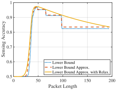
(a) Binary classification with $\gamma=5\text{dB}$

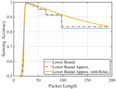
(b) Binary classification with $\gamma=10\text{dB}$

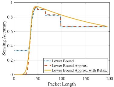
(c) 3 classes with $\gamma=5\text{dB}$

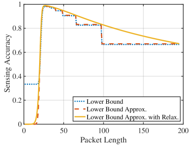
(d) 3 classes with $\gamma=10\text{dB}$

Figure 3: Comparison among lower bound of sensing accuracy $\hat{E}_{\sf{mv}}$ in (19), its approximation in (22) and the approximation with relaxation in (37) in case of multi-view sensing. The settings are $T=1$ms, $\Delta_{S}=0.02$ms, $B_{W}=0.2$MHz, $\xi_{a}=0.95$, $G=1,N=10,Q_{B}=8,\eta=1.7$.

By relaxing the constraint of $[\cdot]_{(1/L)^{+}}$ in the lower bound on classification accuracy, we obtain the following insightful approximation on (19) that follows directly from the application of first-order Taylor expansion around the mean of the random variable $|\hat{\mathcal{K}}|$:

$$\mathbb{E}_{|\hat{\mathcal{K}|}}\left[Q\left(-G\sqrt{|\hat{\mathcal{K}}|}\right)\right]\approx Q\left(-G\sqrt{\mathbb{E}[|\hat{\mathcal{K}}|]}\right).$$ (21)

Using this, the lower bound of sensing accuracy for multi-view sensing in (19), i.e., $\hat{E}_{\sf{mv}}$, can be approximated as

$$\begin{split}\hat{E}_{\sf{mv}}\approx(L-1)Q(-G\sqrt{K_{\sf{mv}}\rho})-(L-2),\end{split}$$ (22)

where $G=\frac{1}{2}\sqrt{g_{\min}}$ and $K_{\sf{mv}}\rho$ is the expected number of successfully transmitted views given a total of $K$ transmissions and successful transmission probability $\rho$. Fig. 3 compares $\hat{E}_{\sf{mv}}$ in (19) to its approximation in (22). For the binary classifier (see Fig. 3(a) and 3(b)), it can be seen that the approximation error is generally very small. The small error stems from the higher-order moments of $|\hat{\mathcal{K}}|$ and has negligible effects on the packet length optimization. For the 3-class classifier (see Fig. 3(c) and 3(d)), the approximation error is also small, except for small packet lengths where the relaxation of the constraint of $[\cdot]_{(1/L)^{+}}$ causes a relatively large error.

Remark 3 (Reliability-View Tradeoff).

The approximation of the lower bound on sensing accuracy in (22) demonstrates the tradeoff between communication reliability and the number of transmitted views. Specifically, $Q(-G\sqrt{x})$ is a monotonically increasing function of $x$. As shown in Fig. 3, regardless of the steps resulting from the integer relaxation of $K_{\sf{mv}}$, an increasing packet length causes two opposite effects on sensing accuracy: by lengthening the packets, the total number of views decreases (i.e., reducing the classification accuracy due to fewer sensor views) while the successful decoding probability increases (i.e., improved communication reliability). This necessitates the optimization of the packet length, as in the case of multi-snapshot sensing.

IV Packet-Length Optimization for Ultra-LoLa Inference

In this section, the packet length that controls the reliability-view tradeoff is optimized to maximize the E2E sensing accuracy by deriving accurate, tractable surrogates of the sensing accuracies. We treat the two sensing scenarios sequentially.

IV-A Optimal Packet-Length for Multi-Snapshot Sensing

We start by optimizing the tradeoff from Proposition 1 to maximize the lower bound on sensing accuracy of multi-snapshot case. First, by expanding $K_{\sf{ms}}$ with the expression in (17), the lower bounded sensing accuracy is a function of the packet length $D$, denoted as $\Psi_{\sf{ms}}(D)$, given as

$$\small\begin{split}\Psi_{\sf{ms}}(D)&=\\ &(L-1)\rho\left[\frac{1}{L}-Q\left(G\sqrt{\left\lfloor\frac{T}{\Delta_{S}}-\frac{D}{B_{W}\Delta_{S}}\right\rfloor}\right)\right]_{(1/L)^{+}}+\frac{1}{L},\end{split}$$ (23)

where $G=\frac{1}{2}\sqrt{g_{\min}}$. The resulting optimization problem for the $L$-class classifier is

$$\begin{split}\max_{D\in\mathbb{Z}_{+}}&\quad\Psi_{\sf{ms}}(D),\end{split}$$ (24)

where $\mathbb{Z}_{+}$ denotes the set of positive integers. In order to solve the problem, we first approximate the Q-function as [30]

$$Q(x)\approx 1-\sigma(\eta x),$$ (25)

where $\sigma(x)=\frac{1}{1+e^{-x}}$ is the sigmoid function and $\eta>0$ is a fitting coefficient. Throughout the paper, we will use $\eta=1.7$, which generally results in a good approximation for a wide range of $x$ [30]. Next, the integer constraint on $K_{\sf{ms}}$ is relaxed by allowing it to take non-integral values, and finally we note that the function $[\cdot]_{{1/L}^{+}}$ in (23) with the approximation in (25) can be replaced by an upper bound on $D$ given by

$$D_{\max}=\left\lfloor\left(T-\frac{\Delta_{S}(\ln{(L-1)})^{2}}{G^{2}\eta^{2}}\right)B_{W}\right\rfloor,$$ (26)

i.e., we constrain $D\in\{1,2,\ldots,D_{\max}\}$.

Using the relaxations above, we obtain the surrogate objective of problem (24), denoted as $\tilde{\Psi}_{\sf{ms}}(D)$, given as

$$\tilde{\Psi}_{\sf{ms}}(D)=\xi_{a}(L-1)\tilde{\nu}_{\sf{ms}}(D)+\frac{1}{L},$$ (27)

where $\tilde{\nu}_{\sf{ms}}(D)$ is a positive function of $D\in\{1,\ldots,D_{\max}\}$, given as

$$\tilde{\nu}_{\sf{ms}}(D)=\left(\sigma\left(\psi_{I}(D)\right)-\frac{L-1}{L}\right)\sigma(\psi_{T}(D)).$$ (28)

The functions $\psi_{I}(D)$ and $\psi_{T}(D)$ are defined as

$$\begin{split}\psi_{I}(D)&=G\eta\sqrt{\frac{T}{\Delta_{S}}-\frac{D}{\Delta_{S}B_{W}}},\\ \psi_{T}(D)&=\ln(2)\eta\sqrt{\frac{D}{V}}\left(\log_{2}(1+\gamma)-\frac{Q_{B}N}{D}\right).\end{split}$$ (29)

As shown in Fig. 4, the proposed function $\tilde{\Psi}_{\sf{ms}}(D)$ provides a good approximation of the lower bound of sensing accuracy $\Psi_{\sf{ms}}(D)$. Building on this approximation, we seek the value of $D$ that maximizes $\tilde{\Psi}_{\sf{ms}}(D)$. Since $\tilde{\Psi}_{\sf{ms}}(D)$ is a monotonically increasing function of $\tilde{\nu}_{\sf{ms}}(D)$, the optimal value of $D$ can be found by solving the simplified problem:

$$\begin{split}\max_{D}&\quad\tilde{\nu}_{\sf{ms}}(D)\\ \text{s.t.}\quad&D\in\{1,2,\dots,D_{\max}\}.\end{split}$$ (30)

$\tilde{\nu}_{\sf{ms}}(D)$ in problem (30) is found to be a log-concave function of $D$ with a unique maximum elaborated in Proposition 2.

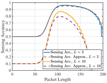
(a) Low SNR with $\gamma=0\text{dB}$

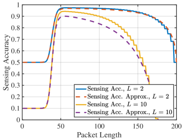
(b) High SNR with $\gamma=5\text{dB}$

Figure 4: Comparison between (23) and its approximation (27) in case of multi-snapshot sensing. The settings are identical to that of multi-view case in Fig. 3 except $G=0.5$.

Proposition 2 (Optimal Packet Length for Multi-Snapshot Sensing).

Let

$$\begin{split}\small f_{\bf{ms}}(D)=&C_{\bf{ms}}\sqrt{\frac{B_{W}T}{D}-1}\left(\log_{2}(1+\gamma)+\frac{Q_{B}N}{D}\right)\\ &-\frac{1+e^{\psi_{T}(D)}}{(1+e^{\psi_{I}(D)})(1/L-e^{-\psi_{I}(D)})},\end{split}$$ (31)

where $C_{\bf{ms}}=\frac{\ln(2)}{G}\sqrt{\frac{\Delta_{S}B_{W}}{V}}$ is a positive constant and $\psi_{T}(D),\psi_{I}(D)$ are defined in (29). The optimal packet length that solves problem (30) is then

$$D^{*}=\left\lfloor\tilde{D}^{*}\right\rceil_{\tilde{\nu}_{\sf{ms}}(\cdot)},$$ (32)

where $\lfloor x\rceil_{\tilde{\nu}_{\sf{ms}}(\cdot)}$ is equal to $\lfloor x\rfloor$ if $\tilde{\nu}_{\sf{ms}}(\lfloor x\rfloor)\geq\tilde{\nu}_{\sf{ms}}(\lceil x\rceil)$, and is otherwise equal to $\lceil x\rceil$, and $\tilde{D}^{*}$ is given as

$$\tilde{D}^{*}=\left\{D|f_{\bf{ms}}(D)=0,D\in[1,D_{\max}]\right\}$$ (33)

if $f_{\bf{ms}}(1)\cdot f_{\bf{ms}}(D_{\max})<0$ holds, otherwise $\tilde{D}^{*}=\operatorname*{argmax}_{D\in\{1,D_{\max}\}}\tilde{\nu}_{\sf{ms}}(D)$.

The proof is given in Appendix B.

Fig. 5 compares the ultra-LoLa packet length obtained using Proposition 2 to the optimal solution of $\Psi_{\sf{ms}}(D)$. The approximations are close to the optimal ones, which validates the surrogate objective function as an accurate approximation. The figure also shows that the optimal balance between communication reliability and classification accuracy is controlled by the SNR and the number of classes $L$. On the one hand, the optimal packet length decreases as the SNR increases, allowing for more snapshots and a higher classification accuracy. On the other hand, increasing the number of classes decreases the optimal packet length as more snapshots are required for a classification task with more classes.

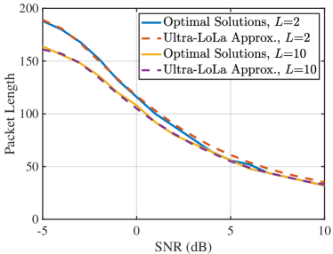
(a) Optimal packet length vs. SNR

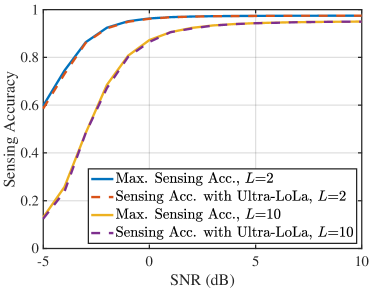
(b) Sensing accuracy vs. SNR

Figure 5: Comparison between optimal solutions and approximated solutions using ultra-LoLa scheme in the case of multi-snapshot sensing with the same setting as Fig. 4.

IV-B Optimal Packet-Length for Multi-View Sensing

We now turn to the problem of choosing the optimal packet length of multi-view sensing. First, we expand $K_{\sf{mv}}$ in (22) with expression in (20) and formulate the optimization problem of interest, given as

$$\begin{split}\max_{D\in\mathbb{Z}_{+}}&\quad\Psi_{\sf{mv}}(D),\end{split}$$ (34)

where $\Psi_{\sf{mv}}(D)$ is the approximation of the lower bounded sensing accuracy:

$$\Psi_{\sf{mv}}(D)=(L-1)Q(-G\sqrt{\nu_{\sf{mv}}(D)})-(L-2),$$ (35)

with $\nu_{\sf{mv}}(D)$ being the expected number of successfully transmitted views, given as

$$\nu_{\sf{mv}}(D)=\left\lfloor\frac{(T-\Delta_{S})B_{W}}{D}\right\rfloor\rho.$$ (36)

Next, we apply again the approximation of Gaussian Q-function in (25) and a relaxation of an integral number of sensors. With the relaxation and approximation above, we obtain the surrogate objective function of problem (34), denoted as $\tilde{\Psi}_{\sf{mv}}(D)$, given as

$$\tilde{\Psi}_{\sf{mv}}(D)=(L-1)Q(-G\sqrt{\tilde{\nu}_{\sf{mv}}(D)})-(L-2),$$ (37)

where $\tilde{\nu}_{\sf{mv}}(D)$ is the approximation of the expected number of received views, given as

$$\tilde{\nu}_{\sf{mv}}(D)=\frac{(T-\Delta_{S})B_{W}\xi_{a}}{D\left(1+\exp(-\psi_{T}(D))\right)},$$ (38)

with $\psi_{T}(D)$ defined in (29).

The approximation error of the approximate sensing accuracy is illustrated in Fig. 3. It is seen that the continuous relaxation in (37) captures the monotonicity and approximates the optimum of the exact expression. Using this approximation, we optimize the packet length $D$ to maximize $\tilde{\Psi}_{\sf{mv}}(D)$. Since $Q(-G\sqrt{x})$ is a monotonically increasing function of $x$, the optimization problem on $\tilde{\Psi}_{\sf{mv}}(D)$ reduces to

$$\begin{split}\max_{D}&\quad\tilde{\nu}_{\sf{mv}}(D)\\ \text{s.t.}\quad&D\in\{1,2,\dots,D_{\max}\},\end{split}$$ (39)

where $D_{\max}=\left\lfloor(T-\Delta_{S})B_{W}\right\rfloor$ is the maximum packet length ensuring $K\geq 1$ (clearly, $K=0$ can never be better than $K\geq 1$).

Finally, $\tilde{\nu}_{\sf{mv}}(D)$ is found to be an unimodal function of $D\in[1,D_{\max}]$ with a unique maximum. Considering the feasible packet length $D\in\{1,\ldots,D_{\max}\}$, the optimal packet length of problem (39), denoted as $D^{*}$, is in the interior of the interval if and only if the derivative of $\tilde{\nu}_{\sf{mv}}(D)$ at the two boundary points have different signs. This is satisfied when

$$f_{\bf{mv}}(1)\cdot f_{\bf{mv}}(D_{\max})<0,$$ (40)

where $f_{\bf{mv}}(D)$ is a function of $D$, given as

$$f_{\bf{mv}}(D)=\frac{\eta\ln(2)\left(\log_{2}(1+\gamma)+NQ_{B}/D\right)}{2\sqrt{DV}(\exp(\psi_{T}(D))+1)}-\frac{1}{D}.$$ (41)

Otherwise, the optimal packet length is obtained at the endpoints, i.e.,

$$D^{*}={\operatorname*{argmax}}_{D\in\{1,D_{\max}\}}\tilde{\nu}_{\sf{mv}}(D).$$ (42)

The optimal packet length given that condition (40) is satisfied is presented in Proposition 3.

Proposition 3 (Optimal Packet Length for Multi-View Sensing).

If the condition in (40) is satisfied, the optimal packet length $D^{*}$ can be obtained as

$$D^{*}=\left\lfloor\frac{V\zeta^{2}}{\ln^{2}(2)\eta^{2}\log^{2}_{2}(1+\gamma)}\right\rceil_{\tilde{\nu}_{\sf{mv}}(\cdot)},$$ (43)

where $\lfloor x\rceil_{\tilde{\nu}_{\sf{mv}}(\cdot)}$ is equal to $\lfloor x\rfloor$ if $\tilde{\nu}_{\sf{mv}}(\lfloor x\rfloor)\geq\tilde{\nu}_{\sf{mv}}(\lceil x\rceil)$, and is otherwise equal to $\lceil x\rceil$, and $\zeta$ is the solution to the transcendental equation

$$\zeta=\left\{x|x+\frac{\omega}{x}-2\exp{\left(x-\frac{\omega}{x}\right)}=2,x>0\right\},$$ (44)

with $\omega=\frac{\ln^{2}(2)\eta^{2}}{V}\log^{2}_{2}(1+\gamma)NQ_{B}$ being a constant representing the effects of channel reliability and sensing quality.

The proof is given in Appendix C.

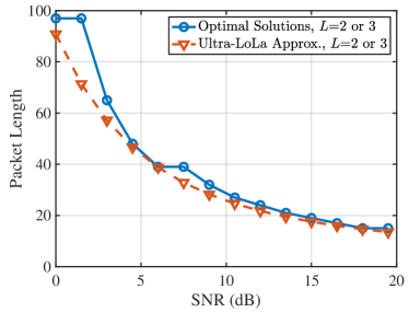
(a) Optimal packet length vs. SNR

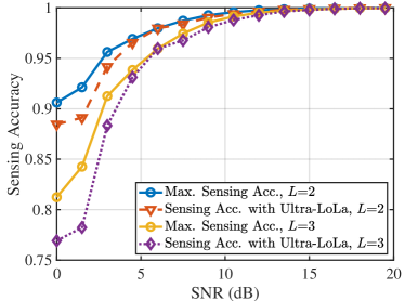
(b) Sensing accuracy vs. SNR

Figure 6: Comparison between optimal solutions and approximate solutions using ultra-LoLa scheme in case of multi-view sensing and the same settings as Fig. 3.

Fig. 6 compares the ultra-LoLa packet length obtained by solving the equation in Proposition 3 to the optimal solution in the settings of SNR and number of classes. Specifically, Fig. 6(a) demonstrates the trend of decreasing optimal packet length with the growth of SNR. This is because that the improvement in packet decoding from increasing SNR can allow shorter packets such that more sensors can be scheduled before the end of the task. Otherwise, the approximate solution is seen to be smaller than the optimal counterpart. The reason is that the optimal packet length guaranteeing an integer total number of sensors is larger than its relaxation. Additionally, both 3-class and binary classification tasks have the same solutions since Problem (39) targets maximizing the expected number of active sensors $\tilde{\nu}_{\sf{mv}}(D)$, which is independent of the number of classes. Correspondingly, in Fig. 6(b), the sensing accuracy with the approximate solution is observed to approach its optimal counterpart with a shrinking gap as the SNR increases. Overall, both an increase in SNR and a decrease in the number of classes enhance the E2E performance due to higher successful decoding probability and an easier classification task, respectively.

V Experimental Results

In this section, we demonstrate the advantages of the proposed framework through numerical results. We first outline the setup, followed by results for linear classification with the GMM. Finally, we demonstrate how the framework performs in MVCNN-based classification.

V-A Experimental Setup

Unless specified otherwise, the experimental settings are set as follows.

V-A1 System and Communication Settings

We consider a single sensor and $K$ distributed sensors for multi-snapshot and multi-view sensing, respectively. For each sensor, we fix the activation probability to $\xi_{a}=1-10^{-5}$ that guarantees the ultra-reliable communication required by URLLC. A total communication bandwidth of $B_{W}=100$ kHz is considered for packet transmission via the access protocols outlined in Section II-D. The packet decoding error probability is assumed to be determined by (9).

V-A2 Sensing and Classification Settings

We consider a very stringent URLLC task completion deadline of $T=1$ms (encompassing both sensing and feature transmission phases) and a sensing time of $\Delta_{S}=0.1$ ms (representing, for instance, an industrial-level camera [31]). To meet the strict deadline, we assume a quantization resolution of 4 bits per feature entry, which has proven to be sufficient for the considered inference tasks and is also consistent with the literature [32]. The linear and MVCNN classifiers are specified below.

• Linear Classification on Synthetic GMM Data: For the linear GMM classifier, we extract feature vectors according to (2) with $L=2,5,10$ classes (selected to vary the classification complexity) and the feature dimensionality set to $N=20$. The centroids of the $L$ clusters are specified as follows: for class $\ell$ ($\ell=1,\ldots,L$), the elements from dimension $N(\ell-1)/L$ to dimension $N\ell/L$ are set to $-1$, while the remaining dimensions are set to $+1$. The covariance matrix is defined as $\mathbf{C}=3\mathbf{I}_{N}$.

• Non-Linear MVCNN-Based Classification on Real-World Data: For the MVCNN classifier, we consider the well-known ModelNet dataset [16], which comprises multi-view images of objects (e.g., a person or a plant), and the popular VGG16 model [33] to implement the MVCNN architecture. We adapt the VGG16 model for our purposes by separating it into feature extractor and classifier networks, with the classifier running on the server and the feature extractor running on the sensors as in [23]. The resulting MVCNN architecture is trained for average pooling and targets a subset of ModelNet, comprising $L=20$ popular object classes. To simulate the sensing phase, each of the $K$ sensors randomly draws an image (view) of the same class (selected uniformly at random) from the dataset. To reduce the communication overhead, each ModelNet image is resized from $3\times 224\times 224$ to $3\times 56\times 56$ (i.e., reducing the image resolution) and fed into the on-device feature extractor, resulting in a $512\times 1\times 1$ tensor. This tensor is then further compressed by a fully connected layer to obtain an output feature vector of dimension $N=20$.

V-A3 Benchmarks

We consider the following benchmarks:

• Brute-force Search: The optimal packet length is obtained by an exhaustive search among all feasible solutions to guarantee the maximum sensing accuracy.

• URLLC: The packet length is determined by computing the shortest packet meeting the decoding error threshold of $10^{-5}$ commonly required in URLLC [7].

• Shannon Rate: The packet length, denoted as $D_{\sf{sr}}$, is determined based on the Shannon rate at the target SNR, i.e., $D_{\sf{sr}}=\left\lceil\frac{NQ_{B}}{\log_{2}(1+\gamma)}\right\rceil$.

Given the task deadline of $T=1$ ms and pre-defined packet lengths in the URLLC and Shannon rate baselines, the number of views for multi-snapshot and multi-view sensing is maximized with respect to (17) and (20), respectively.

V-B Ultra-LoLa Inference with Linear Classification

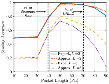
(a) Multi-snapshot sensing (SNR = 5dB)

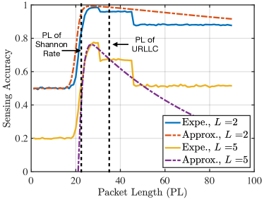
(b) Multi-view sensing (SNR = 10dB)

Figure 7: Packet length versus sensing accuracy for linear classification.

We start by presenting the derived reliability-view tradeoffs. Fig. 7 compares the approximation of sensing accuracy in (27) and (37) with their ground truth in linear classification for a variable packet length. For binary classification (i.e., $L=2$), the approximation can be seen to closely approximate the experimental performance across all packet lengths as also suggested by Remark 1. For the multi-class classifier (i.e., $L=5$), the proposed approximation captures the relationship between the sensing accuracy and the packet length, suggesting that the approximation serves as a good surrogate for the sensing accuracy in the packet-length optimization. Furthermore, the sensing accuracy is seen to increase and then decrease as the packet length increases, revealing the fundamental tradeoff between communication reliability and the number of views. Specifically, when the packet is long, the communication reliability is high, but the number of views is small (i.e., limiting the sensing quality). On the other hand, a short packet has low communication reliability but allows for many views (high sensing quality). Note that the packet lengths obtained using both URLLC and Shannon rate cannot attain the optimal performance. This is because the Shannon rate ignores the communication error caused by the finite blocklength, while URLLC ignores the sensing quality.

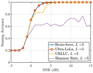
(a) Multi-snapshot sensing ($L=5$)

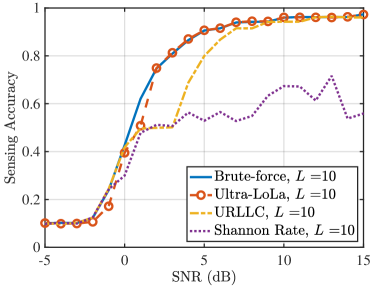
(b) Multi-snapshot sensing ($L=10$)

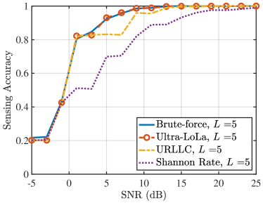
(c) Multi-view sensing ($L=5$)

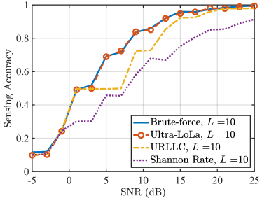
(d) Multi-view sensing ($L=10$)

Figure 8: Sensing accuracy comparison with benchmarks in the case of linear classification.

Fig. 8 shows the sensing accuracy of ultra-LoLa inference as a function of SNR. The sensing accuracy of the ultra-LoLa packet length approaches the brute-force results, rising with the SNR and decreasing with the number of classes. The reasons are twofold: First, a higher SNR leads to a lower decoding error rate, allowing the packet length to be reduced to include for more snapshots (or views) and the sensing quality. Second, with a fixed feature size and covariance matrix, a larger number of classes gives a smaller pair-wise discrimination gain, which compromises classification accuracy.

In Fig. 8, we then compare ultra-LoLa inference with benchmarks in the case of linear classification. The ultra-LoLa scheme achieves similar accuracies as benchmarks when SNR is lower than 0 dB due to the high packet error probability. Compared with URLLC, the multi-view gain can be seen in the SNR range of 0-10 dB for multi-snapshot sensing and 3-20 dB for multi-view sensing. In this regime, ultra-LoLa inference includes more views at the cost of a higher decoding error rate, while URLLC requiring ultra-reliable communication transmits fewer views due to a lower rate. For a high SNR, the required packet length of URLLC decreases, allowing more views to be included, which improves the sensing accuracy and results in a similar performance as ultra-LoLa inference. Moreover, in the multi-snapshot case, there is a significant performance gap between ultra-LoLa and Shannon-rate schemes at high SNR. The reason is that the high decoding error rate associated with the Shannon rate (around 0.5) becomes the bottleneck when all sensing information is transmitted in a single packet. This phenomenon is less significant in multi-view sensing due to view diversity [34].

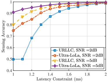
(a) Multi-snapshot sensing

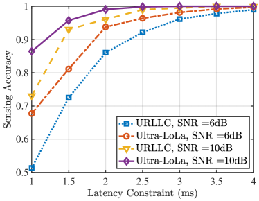
(b) Multi-view sensing

Figure 9: Sensing accuracy versus latency constraints in the case of 10-class linear classifier.

In Fig. 9, the E2E performance of ultra-LoLa inference is measured by the E2E latency constraint and compared with the benchmarks. Relaxing the latency constraint leads to an increase in sensing accuracy by allowing for longer packets and more views. It is observed that the gap between ultra-LoLa inference and the benchmarks is significant under strict latency constraints, showcasing the importance of balancing communication reliability and sensing quality. Additionally, for a given target sensing accuracy, ultra-LoLa inference attains lower latency compared to other schemes.

V-C Ultra-LoLa Inference with MVCNN-Based Classification

We now apply the proposed framework for MVCNN-based classification of a real dataset. We first optimize the packet length exploiting the insights from the linear classifier, and then compare the results to the benchmarks.

V-C1 Packet Length Optimization on Real Dataset

To optimize the packet length of MVCNN, we employ the solution in Proposition 3 for multi-view sensing, while there is no theoretical solution for multi-snapshot sensing due to the unknown minimum discrimination gain of the MVCNN. To tackle this challenge, we propose a lookup-table-based packet length optimization that exploits the insights from the linear classifier. Specifically, leveraging the linear relation between number of views and the packet length in (17), we generate a table of packet lengths and corresponding training accuracy, denoted as $\Psi_{\sf{cnn}}(D)$, during training of the VGG16 using the training dataset. The successful transmission probability can be expressed as a function of packet length with respect to the SNR, feature size, and quantization resolution using (10). Then we estimate the sensing accuracy of the MVCNN with the expectation of $\Psi_{\sf{cnn}}(D)$ over the decoding process, i.e., $\rho\Psi_{\sf{cnn}}(D)+\frac{(1-\rho)}{L}$. In such manner, the packet length of ultra-LoLa inference can be estimated offline by an exhaustive search over the estimated sensing accuracy.

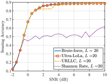
(a) Multi-snapshot sensing

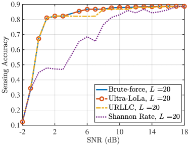
(b) Multi-view sensing

Figure 10: Sensing accuracy comparison with benchmarks in case of MVCNN-based classification.

V-C2 Comparison with Benchmarks

Figs. 10 and 11 demonstrate the performance of ultra-LoLa inference in comparison to the benchmarks in terms of sensing accuracy, latency and SNR. As discussed for linear classification, similar trends can be observed in the MVCNN classifier. For example, a multi-view gain between ultra-LoLa inference and URLLC can be observed at the SNR range of 1–4dB and 3–8dB for the two cases, respectively. Among others, ultra-LoLa inference matches the brute-force results for all settings due to accurate prediction on the training dataset during model training. Without this advantage, URLLC and Shannon rate fail to obtain the maximum performance at the same SNR settings. In addition, as shown in Fig. 11, relaxing the latency constraint allows a larger packet length and a larger number of views, boosting the sensing accuracy as for linear classification.

VI Conclusion

In this paper, we have presented the framework of ultra-LoLa edge inference for latency-constrained distributed sensing. The framework harnesses the interplay between SPT and accuracy improvements from multi-view sensing to meet a stringent deadline while boosting the E2E sensing performance. Under the latency constraint, a fundamental tradeoff between communication reliability and the number of views, controlled by the packet length, is revealed and optimized. The optimization is tackled by deriving accurate surrogate functions of the expressions for the E2E sensing accuracy.

This work is the first to study SPT in edge inference for distributed sensing, opening a number of opportunities for follow-up studies. One direction is accuracy enhancement and latency reduction via joint optimization of packet length and coding rate. This requires further work on characterizing the effects of feature dimensionality and quantization on packet length selection. In terms of energy-efficient communication, it is interesting to design power control techniques that adapt to both fading channels and feature importance. Additionally, the development of the ultra-LoLa inference to incorporate AirComp warrants further investigation.

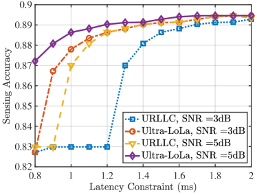
(a) Multi-snapshot sensing

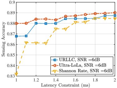
(b) Multi-view sensing

Figure 11: Sensing accuracy versus latency constraints in the case of 20-class MVCNN classifier.

Appendix A Proof of Lemma 1

Conditioned on successful transmission, the inference accuracy with $K$ observations is given as

$$\small A=\frac{1}{L}\sum_{\ell=1}^{L}\Pr(\hat{\ell}=\ell|\ell,K),$$ (45)

where $\Pr(\hat{\ell}=\ell|\ell,K)$ is the correct classification probability given $K$ observations and ground-truth label $\ell$. Following the observation model in (2), the conditional distribution of the fused feature vector $\overline{\mathbf{x}}$ defined in (5) given $\ell$ is $\overline{\mathbf{x}}\sim\mathcal{N}(\boldsymbol{\mu}_{\ell},K^{-1}\mathbf{C})$.

Considering the Mahalanobis distance minimization classifier in (4), the probability of correct classification is

$$\Pr(\hat{\ell}=\ell|\ell,K)=\Pr\left(\cap_{\ell^{\prime}=1,\,\ell^{\prime}\neq\ell}^{L}\left\{z_{\ell}(\overline{\mathbf{x}}|\ell)<z_{\ell^{\prime}}(\overline{\mathbf{x}}|\ell)\right\}\right),$$ (46)

where $z_{\ell^{\prime}}(\overline{\mathbf{x}}|\ell)=(\overline{\mathbf{x}}-\boldsymbol{\mu}_{\ell^{\prime}})^{\sf{T}}\mathbf{C}^{-1}(\overline{\mathbf{x}}-\boldsymbol{\mu}_{\ell^{\prime}})$ is the squared Mahalanobis distance between $\overline{\mathbf{x}}$ and class $\ell^{\prime}$ given that the ground-truth class is $\ell$. Defining the differential squared Mahalanobis distance as $\delta_{\ell,\ell^{\prime}}=z_{\ell}(\overline{\mathbf{x}}|\ell)-z_{\ell^{\prime}}(\overline{\mathbf{x}}|\ell)$, we have

$$\begin{split}\small\Pr(\hat{\ell}=\ell|\ell,K)&=\Pr\left(\cap_{\ell^{\prime}=1,\,\ell^{\prime}\neq\ell}^{L}\left\{\delta_{\ell,\ell^{\prime}}<0\right\}\right)\\ &=1-\Pr\left(\cup_{\ell^{\prime}=1,\,\ell^{\prime}\neq\ell}^{L}\left\{\delta_{\ell,\ell^{\prime}}\geq 0\right\}\right)\\ &\geq 1-\sum_{\ell^{\prime}=1,\,\ell^{\prime}\neq\ell}^{L}\Pr\left(\delta_{\ell,\ell^{\prime}}\geq 0\right)\\ &\geq 1-(L-1)\max_{\forall\ell,\ell^{\prime}}\Pr\left(\delta_{\ell,\ell^{\prime}}\geq 0\right).\end{split}$$ (47)

Denoting by $\overline{\mathbf{x}}_{\ell}(n)$ the $n$-th entry of $\overline{\mathbf{x}}$ when the ground-truth class is $\ell$, the differential squared Mahalanobis distance can be further expressed as $\delta_{\ell,\ell^{\prime}}=z_{\ell}(\overline{\mathbf{x}}|\ell)-z_{\ell^{\prime}}(\overline{\mathbf{x}}|\ell)=\sum_{n=1}^{N}\delta_{\ell,\ell^{\prime}}(n)$, where $\delta_{\ell,\ell^{\prime}}(n)$ is the differential distance of the $n$-th dimension, given as

$$\small\delta_{\ell,\ell^{\prime}}(n)=\frac{2}{C_{n,n}}(\boldsymbol{\mu}_{\ell^{\prime}}(n)-\boldsymbol{\mu}_{\ell}(n))\left(\overline{\mathbf{x}}_{\ell}(n)-\frac{1}{2}\left(\boldsymbol{\mu}_{\ell}(n)+\boldsymbol{\mu}_{\ell^{\prime}}(n)\right)\right).$$ (48)

Note that $\delta_{\ell,\ell^{\prime}}(n)\sim\mathcal{N}(-g_{\ell,\ell^{\prime}}(n),4K^{-1}g_{\ell,\ell^{\prime}}(n))$ is Gaussian consdering the linear mapping from $\overline{\mathbf{x}}_{\ell}(n)$. Since the covariance matrix, $\mathbf{C}$, of the observations is diagonal, $\delta_{\ell,\ell^{\prime}}$ is a sum of $N$ independent Gaussian random variables, distributed as

$$\delta_{\ell,\ell^{\prime}}\sim\mathcal{N}(-g_{\ell,\ell^{\prime}},4K^{-1}g_{\ell,\ell^{\prime}}),$$ (49)

where $g_{\ell,\ell^{\prime}}=\sum_{n=1}^{N}g_{\ell,\ell^{\prime}}(n)=[\boldsymbol{\mu}_{\ell}-\boldsymbol{\mu}_{\ell^{\prime}}]^{\sf{T}}\mathbf{C}^{-1}[\boldsymbol{\mu}_{\ell}-\boldsymbol{\mu}_{\ell^{\prime}}]$ is the total discrimination gain between the two classes.

The probability that distance from ground truth label $\ell$ is greater than that of $\ell^{\prime}$, i.e, $\Pr(\delta_{\ell,\ell^{\prime}}\geq 0)$, can then be given as

$$\begin{split}\small\Pr(\delta_{\ell,\ell^{\prime}}\geq 0)&=\int_{0}^{\infty}\mathcal{N}(\delta_{\ell,\ell^{\prime}};-g_{\ell,\ell^{\prime}},4K^{-1}g_{\ell,\ell^{\prime}})d\delta_{\ell,\ell^{\prime}}\\ &=Q\left(\frac{\sqrt{Kg_{\ell,\ell^{\prime}}}}{2}\right).\end{split}$$ (50)

Substituting (50) into (47), we obtain the lower bound of inference accuracy, given as

$$\begin{split}A=\frac{1}{L}\sum_{\ell=1}^{L}\Pr(\hat{\ell}=\ell|\ell)\geq 1-(L-1)Q\left(\frac{\sqrt{Kg_{\min}}}{2}\right),\end{split}$$ (51)

where $g_{\min}=\min\{g_{\ell_{1},\ell_{2}}|\ell_{1},\ell_{2}\in\{1,2,\dots,L\},\ell_{1}\neq\ell_{2}\}$ is the minimum discrimination gain between any two classes. The proof is completed by noting that the accuracy cannot be smaller than $1/L$ (achieved by random guessing). This completes the proof.

Appendix B Proof of Proposition 2

We first show that $\tilde{\nu}_{\sf{ms}}(D)$ is a log-concave function over the continuous (relaxed) domain $D\in[1,D_{\max}]$, and then establish the optimality conditions for the original problem with $D\in\{1,\ldots,D_{\max}\}$.

Define $f_{I}(D)=\sigma(\psi_{I}(D))$ and $f_{T}(D)=\sigma(\psi_{T}(D))$, which are positive functions of $D\in[1,D_{\max}]$. $\tilde{\nu}_{\sf{ms}}(D)$ can then be expressed as

$$\tilde{\nu}_{\sf{ms}}(D)=\left(f_{I}(D)-\frac{L-1}{L}\right)f_{T}(D).$$ (52)

The functions $\psi_{I}(x)$ and $\psi_{T}(x)$ are concave, which can be seen from their negative second-order derivatives. Specifically, for $D\in[1,D_{\max}]$

$$\begin{split}\small\psi^{\prime\prime}_{I}(D)&=-\frac{G\eta}{4\Delta_{S}^{2}B_{W}^{2}}\left(\frac{T}{\Delta_{S}}-\frac{D}{\Delta_{S}B_{W}}\right)^{-\frac{3}{2}}<0,\\ \psi^{\prime\prime}_{T}(D)&=-\frac{\ln(2)\eta}{4\sqrt{V}}D^{-\frac{5}{2}}\left(\log_{2}(1+\gamma)D+3Q_{B}N\right)<0.\end{split}$$ (53)

Similarly, the sigmoid function $\sigma(x)=\frac{1}{1+\exp(-x)}$ is a log-concave and monotonically increasing function of $x$, and thus $f_{I}(D)$ and $f_{T}(D)$ can be proved to be log-concave functions of $D$ [35]. Building on the constraint that classification accuracy is larger than that of random guessing, i.e.,

$$Q\left(G\sqrt{\frac{T}{\Delta_{S}}-\frac{D}{B_{W}\Delta_{S}}}\right)\leq 0.$$ (54)

The packet length is constrained to at most $D_{\max}$ given in (26). Under this constraint, we have $f_{I}(D)-\frac{L-1}{L}>0,\forall D\in[1,D_{\max}]$, and thus $f_{I}(D)-\frac{L-1}{L}$ is also a log-concave function in $D\in[1,D_{\max}]$ (see, e.g., [35, Exercise 3.48]). The products of two log-concave functions is also a log-concave function, and thus $\tilde{\nu}_{\sf{ms}}(D)$ is a log-concave function of $D\in[1,D_{\max}]$. Then considering the monotonicity of $\ln(x)$, the optimal packet length $\tilde{D}^{*}$ of problem (30) can be given as

$$\begin{split}\tilde{D}^{*}&=\operatorname*{argmax}_{D}\tilde{\nu}_{\sf{ms}}(D)\\ &=\operatorname*{argmax}_{D}\ln(\tilde{\nu}_{\sf{ms}}(D))\\ &=\{D|\tilde{\nu}^{\prime}_{\sf{ms}}(D)=0,D\in[1,D_{\max}]\}.\end{split}$$ (55)

Guaranteeing the maximum point reside in $[1,D_{\max}]$ is equivalent to the existence of the zero of continuous function $\tilde{\nu}^{\prime}_{\sf{ms}}(D),\forall D\in[1,D_{\max}]$. Thus, $\tilde{\nu}^{\prime}_{\sf{ms}}(D)$ evaluated at the endpoints must satisfy

$${\tilde{{\nu}}^{\prime}_{\sf{ms}}(1)\cdot\tilde{\nu}}^{\prime}_{\sf{ms}}(D_{\max})<0,$$ (56)

where $\tilde{{\nu}}^{\prime}_{\sf{ms}}(D)$ is the first derivative given as

$$\begin{split}\tilde{{\nu}}^{\prime}_{\sf{ms}}(D)=f_{\sf{pos}}(D)f_{\bf{ms}}(D),\end{split}$$ (57)

with $f_{\sf{pos}}(D)=-\sigma(\psi_{T}(D))(1-\sigma(\psi_{T}(D)))\left(\sigma(\psi_{I}(D))-\frac{L-1}{L}\right)\psi^{\prime}_{I}(D)\geq 0,\forall D\geq 0$, and $f_{\bf{ms}}(D)$ being a function of $D$ determining the sign of $\tilde{{\nu}}^{\prime}_{\sf{ms}}(D)$, given as

$$\begin{split}f_{\bf{ms}}(D)&=-\frac{1+e^{\psi_{T}(D)}}{(1+e^{\psi_{I}(D)})(1/L-e^{-\psi_{I}(D)})}-\underbrace{\frac{\psi^{\prime}_{T}(D)}{\psi^{\prime}_{I}(D)}}_{(a)}.\\ \end{split}$$ (58)

Note that $(a)$ can be expressed as

$$\small\frac{\psi^{\prime}_{T}(D)}{\psi^{\prime}_{I}(D)}=-C_{\bf{ms}}\sqrt{\frac{B_{W}T}{D}-1}\left(\frac{\log_{2}(1+\gamma)D+Q_{B}N}{D}\right),$$ (59)

where $C_{\bf{ms}}=\frac{\ln(2)}{G}\sqrt{\frac{\Delta_{S}B_{W}}{V}}$ is a positive constant. When the inequality $f_{\bf{ms}}(1)\cdot f_{\bf{ms}}(D_{\max})<0$ holds, the optimal packet length $\tilde{D}^{*}$ is obtained by finding the zero point of $f_{\bf{ms}}(\tilde{D}^{*})=0$. Since the problem is log-convex, the optimal integer packet length, denoted as $D^{*}$, can be obtained by simply inspecting the nearest (feasible) integers less than or greater than $\tilde{D}^{*}$ and picking the one that maximizes the objective function $\tilde{\nu}_{\sf{ms}}(D)$. Otherwise, if $f_{\bf{ms}}(1)\cdot f_{\bf{ms}}(D_{\max})\geq 0$, the optimal packet length is one of the endpoints, i.e., $D^{*}=\operatorname*{argmax}_{D\in\{1,D_{\max}\}}\tilde{\nu}_{\sf{ms}}(D)$. This completes the proof.

Appendix C Proof of Proposition 3

First, to find the maximum of $\tilde{\nu}_{\sf{mv}}(D)$ we investigate its monotonicity through its derivative

$$\begin{split}\tilde{\nu}_{\sf{mv}}^{\prime}(D)=&C_{\sf{pos}}\underbrace{\left[-(1+\exp(\psi_{T}(D)))+D\psi^{\prime}_{T}(D)\right]}_{g(D)},\end{split}$$ (60)

where $C_{\sf{pos}}=\frac{(T-\Delta_{S})B_{W}\xi_{a}\sigma(\psi_{T}(D))}{D^{2}(1+\exp{(\psi_{T}(D))})}>0$ is a positive constant. The monotonicity of $\tilde{\nu}_{\sf{mv}}(D)$ thus depends on the sign of $g(D)$ in (60). $g(D)$ can be expanded as

$$\begin{split}\small g(D)=&-\exp{\left[\frac{\ln(2)\eta}{\sqrt{V}}\left(\frac{\log_{2}(1+\gamma)D-Q_{B}N}{\sqrt{D}}\right)\right]}\\ &+\frac{\ln(2)\eta}{2\sqrt{V}}\left(\log_{2}(1+\gamma)\sqrt{D}+\frac{Q_{B}N}{\sqrt{D}}\right)-1.\end{split}$$ (61)

Define the positive constant $\alpha=\frac{\ln(2)\eta}{\sqrt{V}}\log_{2}(1+\gamma)$ such that $g(D)=q\left(\alpha\sqrt{D}\right)$ where

$$\begin{split}q(x)=\frac{1}{2}\left(x+\frac{\omega}{x}\right)-\left(\exp\left(x-\frac{\omega}{x}\right)+1\right),\end{split}$$ (62)

for $x>0$ with $\omega=\frac{\alpha^{2}Q_{B}N}{\log_{2}(1+\gamma)}>1$ being a positive constant. Then the first derivative of $g(D)$ can be obtained as

$$g^{\prime}(D)=\left(\frac{\alpha}{2\sqrt{D}}\right)q^{\prime}(\alpha\sqrt{D}),$$ (63)

where $q^{\prime}(x)$ is the first derivative of $q(x)$ with respect to $x$, given as

$$\begin{split}q^{\prime}(x)&=\frac{1}{2x^{2}}\left[x^{2}-\omega-2(x^{2}+\omega)\exp(x-\frac{\omega}{x})\right]\\ &=\begin{cases}<0,&x\in(0,\sqrt{\omega})\\ <\frac{1}{2x^{2}}\left[-x^{2}-3\omega\right]<0,&x\in[\sqrt{\omega},\infty).\end{cases}\end{split}$$ (64)

Since $q^{\prime}(x)<0$ for $x>0$, this holds for $g^{\prime}(x)$ as well. Thus $g(D)$ is monotonically decreasing in $D\in[1,D_{\max}]$.

Since $g(D)$ is monotonically decreasing, the value $\tilde{D}^{*}$ that maximizes $\tilde{\nu}_{\sf{mv}}^{\prime}(D)$ either satisfies $g(\tilde{D}^{*})=0$, or is one on the boundary of the domain of $D$. The existence of a $D$ that satisfies $g(D)=0$ is guaranteed if and only if $g(1)g(D_{\max})<0$, such that the boundary points of $g(D)$ have different signs. This condition is the same as the one in (40). Thus, assuming that the condition in (40) is satisfied, the optimal packet length, denoted as $D^{*}$, is unique and given by the solution to transcendental equation $q(\hat{x})=0$, i.e.,

$$\hat{x}+\frac{\omega}{\hat{x}}-2\exp{\left(\hat{x}-\frac{\omega}{\hat{x}}\right)}=2.$$ (65)

Finally, the effects of rounding on the choice of integer packet length is the same as discussed in Appendix B, and thus is omitted. This completes the proof.

References

- [1] HUAWEI, “6G: The next horizon from connected people and things to connected intelligence,” 2022. [Online]. Available: https://www-file.huawei.com/-/media/corp2020/pdf/tech-insights/1/6g-white-paper-en.pdf
- [2] J. Park, S. Samarakoon, M. Bennis, and M. Debbah, “Wireless network intelligence at the edge,” Proc. IEEE, vol. 107, no. 11, pp. 2204–2239, 2019.
- [3] G. Zhu, D. Liu, Y. Du, C. You, J. Zhang, and K. Huang, “Toward an intelligent edge: Wireless communication meets machine learning,” IEEE Commun. Mag., vol. 58, no. 1, pp. 19–25, 2020.
- [4] F. Liu et al., “Integrated sensing and communications: Toward dual-functional wireless networks for 6G and beyond,” IEEE J. Sel. Areas Commun., vol. 40, no. 6, pp. 1728–1767, 2022.
- [5] S. Duan et al., “Distributed artificial intelligence empowered by end-edge-cloud computing: A survey,” IEEE Commun. Surveys Tuts., vol. 25, no. 1, pp. 591–624, 2022.
- [6] Global Semiconductor Alliance, “The challenges to achieve level 4/level 5 autonomous driving.” [Online]. Available: https://www.gsaglobal.org/forums/the-challenges-to-achieve-level-4-level-5-autonomous-driving/
- [7] G. Durisi, T. Koch, and P. Popovski, “Toward massive, ultrareliable, and low-latency wireless communication with short packets,” Proc. IEEE, vol. 104, no. 9, pp. 1711–1726, 2016.
- [8] Y. Polyanskiy, H. V. Poor, and S. Verdú, “Channel coding rate in the finite blocklength regime,” IEEE Trans. Inf. Theory, vol. 56, no. 5, pp. 2307–2359, 2010.
- [9] P. Popovski et al., “Wireless access in ultra-reliable low-latency communication (URLLC),” IEEE Trans. Commun., vol. 67, no. 8, pp. 5783–5801, 2019.
- [10] H. Ren, C. Pan, Y. Deng, M. Elkashlan, and A. Nallanathan, “Joint power and blocklength optimization for URLLC in a factory automation scenario,” IEEE Trans. Wireless Commun., vol. 19, no. 3, pp. 1786–1801, 2019.
- [11] Y. Zhao, J. Hu, K. Yang, and X. Wei, “A joint communication and control system for URLLC in industrial IoT,” IEEE Trans. Veh. Technol., vol. 72, no. 11, pp. 15 074–15 079, 2023.
- [12] J. Östman, G. Durisi, E. G. Ström, M. C. Coşkun, and G. Liva, “Short packets over block-memoryless fading channels: Pilot-assisted or noncoherent transmission?” IEEE Trans. Commun., vol. 67, no. 2, pp. 1521–1536, 2018.
- [13] K. F. Trillingsgaard and P. Popovski, “Downlink transmission of short packets: framing and control information revisited,” IEEE Trans. Commun., vol. 65, no. 5, pp. 2048–2061, 2017.
- [14] C. She, C. Yang, and T. Q. Quek, “Joint uplink and downlink resource configuration for ultra-reliable and low-latency communications,” IEEE Trans. Commun., vol. 66, no. 5, pp. 2266–2280, 2018.
- [15] Y. Hu, Y. Zhu, M. C. Gursoy, and A. Schmeink, “SWIPT-enabled relaying in IoT networks operating with finite blocklength codes,” IEEE J. Sel. Areas Commun., vol. 37, no. 1, pp. 74–88, 2018.
- [16] H. Su, S. Maji, E. Kalogerakis, and E. Learned-Miller, “Multi-view convolutional neural networks for 3D shape recognition,” in proc. IEEE Int. Conf. Comput. Vision (ICCV), Santiago, Chile, Dec. 7-13 2015.
- [17] E. Li, L. Zeng, Z. Zhou, and X. Chen, “Edge AI: On-demand accelerating deep neural network inference via edge computing,” IEEE Trans. Wireless Commun., vol. 19, no. 1, pp. 447–457, 2019.
- [18] W. F. Lo, N. Mital, H. Wu, and D. Gündüz, “Collaborative semantic communication for edge inference,” IEEE Commun. Lett., vol. 12, no. 7, pp. 1125–1129, 2023.
- [19] J. Shao and J. Zhang, “Communication-computation trade-off in resource-constrained edge inference,” IEEE Commun. Mag., vol. 58, no. 12, pp. 20–26, 2020.
- [20] Y.-C. Liu, J. Tian, C.-Y. Ma, N. Glaser, C.-W. Kuo, and Z. Kira, “Who2com: Collaborative perception via learnable handshake communication,” in proc. IEEE Int. Conf. Robot. Automat. (ICRA), 2020, pp. 6876–6883.
- [21] Z. Liu, Q. Lan, and K. Huang, “Resource allocation for multiuser edge inference with batching and early exiting,” IEEE J. Sel. Areas Commun., vol. 41, no. 4, pp. 1186–1200, 2023.
- [22] G. Zhu, Y. Wang, and K. Huang, “Broadband analog aggregation for low-latency federated edge learning,” IEEE Trans. Wireless Commun., vol. 19, no. 1, pp. 491–506, 2020.
- [23] Z. Liu, Q. Lan, A. E. Kalør, P. Popovski, and K. Huang, “Over-the-air multi-view pooling for distributed sensing,” IEEE Trans. Wireless Commun., vol. 23, no. 7, pp. 7652–7667, 2024.
- [24] X. Li et al., “Integrated sensing, communication, and computation over-the-air: MIMO beamforming design,” IEEE Trans. Wireless Commun., vol. 22, no. 8, pp. 5383–5398, 2023.
- [25] M. Ye and R. Yang, “Real-time simultaneous pose and shape estimation for articulated objects using a single depth camera,” in proc. IEEE Conf. Comput. Vis. Pattern Recognit. (CVPR), Columbus, OH, USA, Jun. 23–28 2014.
- [26] J. A. Figueroa, “Semi-supervised learning using deep generative models and auxiliary tasks,” in proc. Adv. Neural Inf. Process. Syst. (NeurIPS) Workshop, Vancouver, Canada, Dec. 13–14, 2019.
- [27] Q. Lan, Q. Zeng, P. Popovski, D. Gündüz, and K. Huang, “Progressive feature transmission for split classification at the wireless edge,” IEEE Trans. Wireless Commun., vol. 22, no. 6, pp. 3837–3852, 2023.
- [28] P. Popovski et al., “Wireless access for ultra-reliable low-latency communication: Principles and building blocks,” IEEE Netw., vol. 32, no. 2, pp. 16–23, 2018.
- [29] W. Yang, G. Caire, G. Durisi, and Y. Polyanskiy, “Optimum power control at finite blocklength,” IEEE Trans. Inf. Theory, vol. 61, no. 9, pp. 4598–4615, 2015.
- [30] M. Lopez-Benitez and D. Patel, “Sigmoid approximation to the Gaussian -function and its applications to spectrum sensing analysis,” in proc. IEEE Wireless Commun. Netw. Conf. (WCNC), Marrakech, Morocco, April 15–19 2019.
- [31] G. Weinberg and O. Katz, “100,000 frames-per-second compressive imaging with a conventional rolling-shutter camera by random point-spread-function engineering,” Optics Express, vol. 28, no. 21, pp. 30 616–30 625, 2020.
- [32] X. Sun et al., “Ultra-low precision 4-bit training of deep neural networks,” in proc. Adv. Neural Inf. Process. Syst. (NeurIPS), Dec. 6–12 2020.
- [33] K. Simonyan and A. Zisserman, “Very deep convolutional networks for large-scale image recognition,” in proc. Int. Conf. Learn. Represent., 2015.
- [34] R. Jurdi, S. R. Khosravirad, H. Viswanathan, J. G. Andrews, and R. W. Heath, “Outage of periodic downlink wireless networks with hard deadlines,” IEEE Trans. Commun., vol. 67, no. 2, pp. 1238–1253, 2019.
- [35] S. P. Boyd and L. Vandenberghe, Convex optimization. Cambridge university press, 2004.