H(curl)-based approximation of the Stokes problem with slip boundary conditions

Abstract

The equations governing incompressible Stokes flow are reformulated such that the velocity is sought in the space H(curl). This relaxed regularity assumption leads to conforming finite element methods using spaces common to discretizations of Maxwell’s equations. A drawback of this approach, however, is that it is not immediately clear how to enforce Navier-slip boundary conditions. By recognizing the slip condition as a Robin boundary condition, we show that the continuous system is well-posed, propose finite element methods, and analyze the discrete system by deriving stability and a priori error estimates. Numerical experiments in 2D confirm the derived, optimal convergence rates.

1 Introduction

The vorticity-velocity-pressure (VVP) formulation of the Stokes problem, proposed by Nédélec [28], has been thoroughly studied both theoretically and numerically by Dubois and collaborators [11, 12, 13]. In this formulation, the velocity is sought in either $\mathbf{H}(\operatorname{curl},\Omega)$ or $\mathbf{H}(\operatorname{div},\Omega)$ instead of the more conventional $\mathbf{H}^{1}$ space, which leads to different finite element methods [7]. This formulation is widely used also in the context of the Navier-Stokes equations, see e.g. [18, 38, 36, 21]. However, the VVP formulation has two issues: a slightly suboptimal convergence rate in the case of Dirichlet boundary conditions [4] and it is not immediately clear how to impose Navier slip boundary conditions.

The former issue has been tackled by Salaün and Salmon [33], who restored the optimal convergence rate in the lowest order case by slightly modifying the space in which the vorticity is sought. The main contribution of this work is a solution to the latter issue. In particular, we introduce and analyze a discrete vorticity-velocity-pressure formulation of the Stokes problem with Navier slip boundary condition in which the velocity is sought in a $\mathbf{H}(\operatorname{curl},\Omega)$ conforming space.

We start by formulating the continuous problem and show that it is well-posed using the theory of compact perturbations of coercive operators on the space $\mathbf{X}=\mathbf{H}(\operatorname{curl},\Omega)\cap\nabla H^{1}(\Omega)^{\perp}$. We then consider the discrete setting, for which we cannot directly apply the standard theory, since the discrete space contains elements of $\mathbf{H}(\operatorname{curl},\Omega)$ that are orthogonal only to discrete gradients. The discrete space is thus non-conforming. Fortunately, the discrete and continuous space are shown to be “close enough”  to prove well-posedness and convergence.

The work is organized as follows. In Section 2 we recall how to derive the VVP formulation and an equivalent expression for Navier slip boundary conditions due to Mitrea and Monniaux [26]. In Section 3 we write the continuous variational formulation and show its well-posedness. In Section 4 we focus on the discrete formulation, derive a priori error estimates for its solution, and extend the analytical results to the saddle-point system involving the pressure. Finally, in Section 5 we validate our new method against five numerical test cases.

2 The Stokes problem in rotation form with slip boundary condition

Let $\Omega\subset\mathbb{R}^{d}$, $d=2,3$ be a bounded Lipschitz or smooth domain and denote by $\Gamma$ its boundary. Formally, we seek a velocity field $\mathbf{u}:\Omega\to\mathbb{R}^{d}$ and pressure field $p:\Omega\to\mathbb{R}$ such that

$$-2\nabla\cdot\boldsymbol{\varepsilon}(\mathbf{u})+\nabla p =\mathbf{f}, \Omega,$$ in (2.1a)

$$\nabla\cdot\mathbf{u} =0, \Omega,$$ in (2.1b)

$$\mathbf{u}\cdot\mathbf{n} =0, \Gamma,$$ on (2.1c)

$$[\boldsymbol{\varepsilon}(\mathbf{u})\mathbf{n}]_{\mathrm{tan}} =0, \Gamma,$$ on (2.1d)

where $\mathbf{f}:\Omega\mapsto\mathbb{R}^{d}$ is a given forcing term and $\mathbf{n}:\Gamma\mapsto\mathbb{R}^{d}$ is the outward oriented, unit vector normal to $\Gamma$. Moreover, $\boldsymbol{\varepsilon}(\mathbf{u})$ denotes the symmetric gradient of $\mathbf{u}$, that is,

$$\boldsymbol{\varepsilon}(\mathbf{u})\coloneqq\frac{1}{2}\left(\nabla\mathbf{u}+(\nabla\mathbf{u})^{T}\right).$$ (2.2)

Finally, $\boldsymbol{\zeta}_{\mathrm{tan}}\coloneqq\boldsymbol{\zeta}-(\boldsymbol{\zeta}\cdot\mathbf{n})\mathbf{n}$ denotes the tangential part of a vector field $\boldsymbol{\zeta}$ on $\Gamma$.

Note that rigid body motions may lie in the kernel of Equation 2.1. Consider the disk $\Omega\coloneqq\{(x,y)\in\mathbb{R}^{2};x^{2}+y^{2}\leq 1\}$. Then, the rotation field $\mathbf{u}=[-y,x]^{T}$ is a solution to Equation 2.1 with $\mathbf{f}=\mathbf{0}$. Thus, in general, we need to explicitly assume that the kernel is trivial.

In the case that $\Gamma$ is a $C^{2}$-boundary, Mitrea and Monniaux [26, eq. 2.9] have shown that the homogeneous Navier slip boundary conditions are equivalent to

$$\mathbf{u}\cdot\mathbf{n} =0, -\mathbf{n}\times(\nabla\times\mathbf{u})+2\mathcal{W}(\mathbf{u}_{\mathrm{tan}}) =0,$$ (2.3)

with $\mathcal{W}:T\Gamma\to T\Gamma$ the Weingarten map and $T\Gamma$ the space of tangential vector fields on $\Gamma$.

In the two-dimensional case ($d=2$), the Weingarten map reduces to the scalar curvature of $\Gamma$. Moreover, the curl operator is defined as $\nabla\times\mathbf{u}\coloneqq\partial_{x}u_{y}-\partial_{y}u_{x}$ for vector-valued $\mathbf{u}=[u_{x},u_{y}]^{T}$ and $\nabla\times q\coloneqq[\partial_{y}q,-\partial_{x}q]^{T}$ for scalar $q$.

For sufficiently smooth $\mathbf{u}$ with $\nabla\cdot\mathbf{u}=0$, we can rewrite the second order term in Equation 2.1a as

$$-2\nabla\cdot\boldsymbol{\varepsilon}(\mathbf{u}) =-\Delta\mathbf{u}-\nabla(\nabla\cdot\mathbf{u})$$ (2.4)

$$=\nabla\times\nabla\times\mathbf{u}-2\nabla(\nabla\cdot\mathbf{u})$$

$$=\nabla\times\nabla\times\mathbf{u}.$$

We conclude formally that the solution of the Stokes problem (2.1) satisfies the following problem: find a velocity field $\mathbf{u}:\Omega\to\mathbb{R}^{d}$ and pressure field $p:\Omega\to\mathbb{R}$ such that

$$\nabla\times\nabla\times\mathbf{u}+\nabla p =\mathbf{f}, \Omega,$$ in (2.5a)

$$\nabla\cdot\mathbf{u} =0, \Omega,$$ in (2.5b)

$$\mathbf{u}\cdot\mathbf{n} =0, \Gamma,$$ on (2.5c)

$$-\mathbf{n}\times(\nabla\times\mathbf{u})+\alpha(\mathbf{u}_{\mathrm{tan}}) =0, \Gamma,$$ on (2.5d)

where $\alpha=2\mathcal{W}$. In this work, however, we will consider the more general case in which $\alpha:\Gamma\to\mathbb{R}^{(d-1)\times(d-1)}$ is symmetric and bounded in the $L^{\infty}$ norm. Problem (2.5) will be the starting point for our discretization.

Remark 2.1.

Note that the determinant of the Weingarten map $\mathcal{W}$ is the Gaussian curvature of $\Gamma$. We can therefore not draw conclusions on the sign of $\alpha$ for general $\Omega$. In the case of a convex $C^{1,1}$-domain, for example, $\mathcal{W}(x)$ will be negative semi-definite for all $x\in\Gamma$. In general, however, $\mathcal{W}$ may be positive-definite, negative-definite, or indefinite on various parts of the boundary.

Remark 2.2.

In terms of differential forms, $u$ can be considered a $1$-form or a $(n-1)$-form. Equation (2.5d) then reads either as $-\mathrm{d}u^{\mathrm{nor}}+\alpha u^{\mathrm{tan}}$ or $-\delta u^{\mathrm{tan}}+\alpha u^{\mathrm{nor}}$, respectively. Here $\zeta^{\mathrm{tan}}$ and $\zeta^{\mathrm{nor}}$ denote the tangential and the normal trace of a differential form $\zeta$ respectively, see e.g. [5]. We then immediately see that equation (2.5d) is a Robin boundary condition. This type of boundary conditions has been investigated in finite element exterior calculus by Yang [37], assuming that $\alpha$ is a positive constant and with the boundary condition $p=0$ in place of $\mathbf{u}\cdot\mathbf{n}=0$. Unfortunately, that analysis does not apply to our problem.

Remark 2.3.

Problem (2.5) is similar to the time-harmonic Maxwell equations with impedance boundary conditions [17]. The main difference is the divergence-free constraint which gives additional smoothness to the space in which $\mathbf{u}$ is sought, but makes the analysis of the discrete problem more involved. These two issues will be discussed in Sections 3 and 4, respectively.

Remark 2.4.

The Stokes equations can alternatively be obtained as the incompressible limit of linearized elasticity. In particular, let $\mathbf{u}$ now denote the displacement and define the solid pressure as $p=-\lambda\nabla\cdot\mathbf{u}$ with $\lambda$ the first Lamé parameter. The equations for linearized elasticity with zero traction then read:

$$-\nabla\cdot(2\mu\boldsymbol{\varepsilon}(\mathbf{u})-pI) =\mathbf{f}, \Omega,$$ in (2.6a)

$$\nabla\cdot\mathbf{u}+\lambda^{-1}p =0, \Omega,$$ in (2.6b)

$$\mathbf{u}\cdot\mathbf{n}=0,\quad[\boldsymbol{\varepsilon}(\mathbf{u})\mathbf{n}]_{\mathrm{tan}} =0, \Gamma,$$ on (2.6c)

Using the substutions from (2.3) and (2.4), we note that system (2.5) corresponds to (2.6) for materials with second Lamé parameter $\mu=1$ in the incompressible limit of $\lambda\to\infty$. A similar approach was adopted in [3]. We reserve investigation of this system for future research.

3 Variational formulation of the continuous problem

In this section, we first describe the functional setting and introduce the notation conventions used throughout this work. Afterward, we present and analyze the variational formulation of (2.5).

3.1 Functional Setting

Let $\Omega\subset\mathbb{R}^{d}$, $d=2,3$, be a contractible domain that is either a Lipschitz polygon or has a $C^{1,1}$-boundary. We denote the $L^{2}(\Omega)$ inner product by parentheses and the analogous product on its boundary $\Gamma$ by angled brackets:

$$(\mathbf{u},\mathbf{v}) \coloneqq\int_{\Omega}\mathbf{u}\cdot\mathbf{v}\,\mathrm{dx}, \langle\mathbf{u},\mathbf{v}\rangle \coloneqq\int_{\Gamma}\mathbf{u}\cdot\mathbf{v}\,\mathrm{dS}.$$ (3.1)

With a slight abuse of notation, we denote inner products for scalar functions using the same parentheses and brackets.

We recall the definitions of the following classical Hilbert spaces

$$\mathbf{H}(\operatorname{curl},\Omega) \coloneqq\{\mathbf{v}\in\mathbf{L}^{2}(\Omega)\mid\nabla\times\mathbf{v}\in(L^{2}(\Omega))^{2d-3}\},$$

$$\mathbf{H}(\operatorname{div},\Omega) \coloneqq\{\mathbf{v}\in\mathbf{L}^{2}(\Omega)\mid\nabla\cdot\mathbf{v}\in L^{2}(\Omega)\},$$

and their associated norms

$$\lVert\mathbf{v}\rVert_{\mathbf{H}(\operatorname{curl},\Omega)} \coloneqq\lVert\mathbf{v}\rVert_{\mathbf{L}^{2}(\Omega)}+\lVert\nabla\times\mathbf{v}\rVert_{\mathbf{L}^{2}(\Omega)},$$

$$\lVert\mathbf{v}\rVert_{\mathbf{H}(\operatorname{div},\Omega)} \coloneqq\lVert\mathbf{v}\rVert_{\mathbf{L}^{2}(\Omega)}+\lVert\nabla\cdot\mathbf{v}\rVert_{\mathbf{L}^{2}(\Omega)}.$$

We continue by defining the subspaces $\mathbf{H}_{0}(\operatorname{div},\Omega)$ and $\mathbf{H}_{0}(\operatorname{div}_{0},\Omega)$ as

$$\mathbf{H}_{0}(\operatorname{div},\Omega) \coloneqq\{\mathbf{v}\in\mathbf{H}(\operatorname{div},\Omega)\mid\mathbf{v}\cdot\mathbf{n}=0\},$$

$$\mathbf{H}_{0}(\operatorname{div}_{0},\Omega) \coloneqq\{\mathbf{v}\in\mathbf{H}_{0}(\operatorname{div},\Omega)\mid\nabla\cdot\mathbf{v}=0\},$$

which are well defined by [19, Thm. 2.5].

For function spaces with regularity of fractional order, we will use the Sobolev-Slobodeckij norm for $s>0$:

$$\lvert\mathbf{v}\rvert_{\mathbf{H}^{s}(\Omega)}\coloneqq\left(\int_{\Omega}\int_{\Omega}\frac{\lvert\mathbf{v}(\mathbf{x})-\mathbf{v}(\mathbf{y})\rvert^{2}}{\lVert\mathbf{x}-\mathbf{y}\rVert^{2s+d}}\,d\mathbf{x}\,d\mathbf{y}\right)^{\frac{1}{p}}.$$ (3.2)

The analogous definition holds when the norm is considered on $\Gamma$. This allows us to define the spaces

$$\mathbf{H}^{s}(\Omega) \coloneqq\{\mathbf{v}\in\mathbf{L}^{2}(\Omega)\mid\lvert\mathbf{v}\rvert_{\mathbf{H}^{s}(\Omega)}<\infty\},$$ (3.3)

$$\mathbf{H}^{s}_{\parallel}(\Gamma) \coloneqq\{\mathbf{v}\in\mathbf{H}^{s}_{\parallel}(\Gamma)\mid\mathbf{v}\cdot\mathbf{n}=0\}.$$ (3.4)

Similarly, we define

$$\mathbf{L}^{2}_{\parallel}(\Gamma)\coloneqq\{\boldsymbol{\zeta}\in\mathbf{L}^{2}(\Gamma)\mid\boldsymbol{\zeta}\cdot\mathbf{n}=0\}.$$ (3.5)

We are now ready to define the tangential trace operator $\boldsymbol{\gamma}_{\parallel}:\boldsymbol{\mathcal{C}}^{\infty}(\Omega)\to\mathbf{L}^{2}_{\parallel}(\Gamma)$ as

$$\boldsymbol{\gamma}_{\parallel}(\mathbf{v}) \coloneqq\mathbf{n}\times(\mathbf{v}_{\restriction\Gamma}\times\mathbf{n}), \forall\mathbf{v} \in\boldsymbol{\mathcal{C}}^{\infty}(\Omega).$$

Using [16, Thm. 3.10], $\boldsymbol{\gamma}_{\parallel}$ can be extended to a bounded map $\boldsymbol{\gamma}_{\parallel}:\mathbf{H}^{s}(\Omega)\to\mathbf{H}^{s-\frac{1}{2}}_{\parallel}(\Gamma)$ whenever $\frac{1}{2}<s\leq\frac{3}{2}$. On the other hand, it was shown by Buffa, Costabel and Sheen [10] that $\boldsymbol{\gamma}_{\parallel}$ can be extended to a bounded map $\boldsymbol{\gamma}_{\parallel}:\mathbf{H}(\operatorname{curl},\Omega)\to\mathbf{H}^{-\frac{1}{2}}_{\parallel}(\Gamma)$, where $\mathbf{H}^{-\frac{1}{2}}_{\parallel}(\Gamma)$ denotes the dual of $\mathbf{H}^{\frac{1}{2}}_{\parallel}(\Gamma)$. We will make a slight abuse of notation and not distinguish between these two extensions. We summarize these results in the following lemma.

Lemma 3.1.

$\boldsymbol{\gamma}_{\parallel}:\mathbf{H}^{s}(\Omega)\to\mathbf{H}^{s-\frac{1}{2}}_{\parallel}(\Gamma)$, $\frac{1}{2}<s\leq\frac{3}{2}$, and $\boldsymbol{\gamma}_{\parallel}:\mathbf{H}(\operatorname{curl},\Omega)\to\mathbf{H}^{-\frac{1}{2}}_{\parallel}(\Gamma)$ are bounded.

The final space we introduce is $\mathbf{X}\coloneqq\mathbf{H}(\operatorname{curl},\Omega)\cap\mathbf{H}_{0}(\operatorname{div}_{0},\Omega)$, which we equip with the $\mathbf{H}(\operatorname{curl},\Omega)$-norm. Note that $\mathbf{X}$ can equivalently be characterized as

$$\mathbf{X}=\{\mathbf{v}\in\mathbf{H}(\operatorname{curl},\Omega)\mid(\mathbf{v},\nabla q)=0,\forall q\in H^{1}(\Omega)\}.$$ (3.6)

Recall that the Poincaré-Steklov inequality holds on $\mathbf{X}$:

Theorem 3.2.

If $\Omega$ is contractible, then a $C>0$ exists such that for all $\mathbf{v}\in\mathbf{X}$

$$\lVert\mathbf{v}\rVert_{\mathbf{L}^{2}(\Omega)}\leq C\lVert\nabla\times\mathbf{v}\rVert_{\mathbf{L}^{2}(\Omega)}.$$

Proof.

See [15, Lem. 4.2]. ∎

The Poincaré-Steklov inequality implies that the norms $\lVert\cdot\rVert_{X}$ and $\lVert\nabla\times\cdot\rVert_{\mathbf{L}^{2}(\Omega)}$ are equivalent on $\mathbf{X}$. We will use this result throughout this work without explicitly mentioning it. We proceed with some regularity properties.

Theorem 3.3.

If $\Omega$ is a Lipschitz polyhedron, there exists $s>\frac{1}{2}$ such that $\mathbf{X}$ is continuously embedded in $\mathbf{H}^{s}(\Omega)$. If $\Omega$ is either a convex domain or has a $C^{1,1}$ boundary, the above statement holds with $s=1$.

Proof.

See Amrouche et al. [1, Thm. 2.9, 2.17, Prop. 3.7]. ∎

From now on, we will denote by $s>\frac{1}{2}$ the smoothness index of Theorem 3.3. As a consequence of the above theorem, we obtain the following trace inequality in $\mathbf{X}$.

Corollary 3.4.

If $\Omega$ is contractible and either a Lipschitz polyhedron or a domain with $\mathcal{C}^{1,1}$ boundary, then there exists $C>0$ such that for all $\mathbf{v}\in\mathbf{X}$

$$\lVert\boldsymbol{\gamma}_{\parallel}(\mathbf{v})\rVert_{\mathbf{L}^{2}(\Gamma)}\leq C\lVert\nabla\times\mathbf{v}\rVert_{\mathbf{L}^{2}(\Omega)}.$$

Proof.

We have for $\mathbf{v}\in\mathbf{X}$ and $s>\frac{1}{2}$ the smoothness index:

$$\lVert\boldsymbol{\gamma}_{\parallel}(\mathbf{v})\rVert_{\mathbf{L}^{2}(\Gamma)}\leq\lVert\boldsymbol{\gamma}_{\parallel}(\mathbf{v})\rVert_{\mathbf{H}^{s-\frac{1}{2}}_{\parallel}(\Gamma)}\leq C\lVert\mathbf{v}\rVert_{\mathbf{H}^{s}(\Omega)}\leq C\lVert\nabla\times\mathbf{v}\rVert_{\mathbf{L}^{2}(\Omega)},$$

where we used Lemma 3.1 for the second inequality and Theorem 3.3 for the third inequality. ∎

We emphasize that our domain of interest $\Omega$ is contractible by assumption.

3.2 The continuous problem

Multiplying equation (2.5a) by $\mathbf{v}$, integrating by parts and using the boundary condition (2.5d) we obtain the continuous problem: find $\mathbf{u}\in\mathbf{X}$ such that

$$a(\mathbf{u},\mathbf{v}) =(\mathbf{f},\mathbf{v}), \forall\mathbf{v} \in\mathbf{X}.$$ (3.7)

Here we have defined the bilinear forms $\tilde{a},k,a:\mathbf{X}\times\mathbf{X}\to\mathbb{R}$ as

$$a \coloneqq\tilde{a}+k, \tilde{a}(\mathbf{u},\mathbf{v}) \coloneqq(\nabla\times\mathbf{u},\nabla\times\mathbf{v}), k(\mathbf{u},\mathbf{v}) \coloneqq\langle\alpha\boldsymbol{\gamma}_{\parallel}(\mathbf{u}),\boldsymbol{\gamma}_{\parallel}(\mathbf{v})\rangle.$$ (3.8)

We analyze (3.7) showing several key properties of the bilinear forms in the following lemma.

Lemma 3.5.

The bilinear forms $\tilde{a},k$ and $a$ are symmetric and bounded on $\mathbf{X}$. Moreover, $\tilde{a}$ is coercive on $\mathbf{X}$, that is, a $\gamma>0$ exists such that for all $\mathbf{v}\in\mathbf{X}$

$$\tilde{a}(\mathbf{v},\mathbf{v})\geq\gamma\lVert\mathbf{v}\rVert_{X}^{2}.$$ (3.9)

Proof.

The symmetry of the bilinear forms is immediate due to the assumed symmetry on $\alpha$. The boundedness of $\tilde{a}:\mathbf{X}\times\mathbf{X}\to\mathbb{R}$ follows directly from a Cauchy-Schwarz inequality. For boundedness of $k$, we first recall that $\alpha\in(L^{\infty}(\Gamma))^{(d-1)\times(d-1)}$. Let $\mathbf{u},\mathbf{v}\in\mathbf{X}$, then Corollary 3.4 implies,

$$k(\mathbf{u},\mathbf{v}) \leq\lVert\alpha\rVert_{L^{\infty}(\Gamma)}\lVert\boldsymbol{\gamma}_{\parallel}(\mathbf{u})\rVert_{\mathbf{L}^{2}(\Gamma)}\lVert\boldsymbol{\gamma}_{\parallel}(\mathbf{v})\rVert_{\mathbf{L}^{2}(\Gamma)}$$

$$\leq C\lVert\alpha\rVert_{L^{\infty}(\Gamma)}\lVert\nabla\times\mathbf{u}\rVert_{\mathbf{L}^{2}(\Omega)}\lVert\nabla\times\mathbf{v}\rVert_{\mathbf{L}^{2}(\Omega)},$$

Thus, we conclude boundedness of $k:X\times X\to\mathbb{R}$ and thereby $a:X\times X\to\mathbb{R}$. Coercivity of $\tilde{a}:X\times X\to\mathbb{R}$ follows directly from Theorem 3.2. ∎

With Lemma 3.5, we prove the following result.

Theorem 3.6.

The null space

$$W:=\{\mathbf{u}\in X\mid a(\mathbf{u},\mathbf{v})=0,\forall\mathbf{v}\in\mathbf{X}\},$$ (3.10)

is finite-dimensional.

Proof.

Define the operators $A,\tilde{A},K:\mathbf{X}\to\mathbf{X}^{*}$ via

$$\langle A\mathbf{u},\mathbf{v}\rangle_{\ast} \coloneqq a(\mathbf{u},\mathbf{v}), \langle\tilde{A}\mathbf{u},\mathbf{v}\rangle_{\ast} \coloneqq\tilde{a}(\mathbf{u},\mathbf{v}), \langle K\mathbf{u},\mathbf{v}\rangle_{\ast} \coloneqq k(\mathbf{u},\mathbf{v}),$$

for $\mathbf{u},\mathbf{v}\in\mathbf{X}$ and $X^{*}$ the dual of $X$. Lemma 3.5 implies that $\tilde{a}$ is coercive in $\mathbf{X}$. Therefore the Lax-Milgram theorem [9, Cor. 5.8] implies that $\tilde{A}^{-1}$ exists and is bounded, while the compact embedding of $\mathbf{H}^{s-\frac{1}{2}}_{\parallel}(\Gamma)$ in ${\mathbf{L}^{2}_{\parallel}(\Gamma)}$ [17, Lemma 4.5] implies that $K$ is compact. Therefore [9, Prop. 6.3] implies that $\tilde{A}^{-1}K$ is compact too. The Fredholm alternative [9, Thm. 6.6] then implies that $I+\tilde{A}^{-1}K$ has a finite-dimensional kernel. The statement follows from $A=\tilde{A}(I+\tilde{A}^{-1}K)$. ∎

Remark 3.1.

Theorem 3.6 implies that—if a solution to Problem (3.7) exists—then it is unique up to addition of elements in the finite-dimensional space $W$. Thus, if we moreover assume that $W$ is trivial, then the solution is unique.

Remark 3.2.

If $\alpha$ is positive (semi-)definite, then $W$ is trivial and Problem (3.7) is well-posed by Lax-Milgram. However, as noted in Remark 2.1, $\alpha$ can be a negative or indefinite operator on parts of the boundary, and thus a more involved analysis is required.

Remark 3.3.

It is also possible to consider an alternative variational formulation. Let $\boldsymbol{\omega}\coloneqq\nabla\times\mathbf{u}$ denote the vorticity and assume that $\alpha^{-1}$ exists and is bounded. Then, multiplication by appropriate test functions, integration by parts and boundary condition (2.5d) yield the following variational formulation: find $\boldsymbol{\omega}\in\Sigma$, $\mathbf{u}\in\mathring{\mathbf{H}}(\mathrm{div},\Omega)$ and $p\in L^{2}(\Omega)$ satisfying

$$(\boldsymbol{\omega},\mathbf{z})-(\mathbf{u},\nabla\times\mathbf{z})+\langle\alpha^{-1}\boldsymbol{\gamma}_{\parallel}(\boldsymbol{\omega}),\boldsymbol{\gamma}_{\parallel}(\mathbf{z})\rangle =0,$$

$$(\nabla\times\boldsymbol{\omega},\mathbf{v})-(p,\nabla\cdot\mathbf{v}) =(\mathbf{f},\mathbf{v}),$$

$$(\nabla\cdot\mathbf{u},q) =0,$$

for each $\mathbf{z}\in\Sigma$, $\mathbf{v}\in\mathring{\mathbf{H}}(\mathrm{div},\Omega)$ and $q\in L^{2}(\Omega)$. Here $\Sigma$ is a subspace of $\mathbf{H}(\operatorname{curl},\Omega)$ on which the bilinear forms are well-defined. This formulation is more suitable for $\mathbf{H}(\operatorname{div},\Omega)$-conforming elements for the velocity. We pursue this research in a separate paper.

4 A priori analysis of the discrete problem

Let $\{\Omega_{h}\}_{h}$ be a quasi-uniform and uniformly shape regular family of meshes on $\Omega$ with $h>0$ the mesh size. Let $\Gamma_{h}$ denote the $(d-1)$-dimensional boundary mesh obtained by restricting $\Omega_{h}$ to $\Gamma$.

Let $\mathbf{V}_{h}$ and $Q_{h}$ be piecewise-polynomial subspaces of $\mathbf{H}(\operatorname{curl},\Omega)$ and $H^{1}(\Omega)$ respectively, satisfying $\nabla Q_{h}\subseteq V_{h}$. In turn, the pair of spaces satisfies the following inf-sup condition:

$$\inf_{q_{h}\in Q_{h}}\sup_{\mathbf{v}_{h}\in\mathbf{V}_{h}}\frac{(\nabla q_{h},\mathbf{v}_{h})}{\lVert q_{h}\rVert_{H^{1}(\Omega)}\lVert\mathbf{v}_{h}\rVert_{\mathbf{H}(\operatorname{curl},\Omega)}}\geq\beta>0$$ (4.1)

with $\beta>0$ independent of $h$. We now define the discrete analogue of $\mathbf{X}$ as

$$\mathbf{X}_{h}\coloneqq\{\mathbf{v}_{h}\in\mathbf{V}_{h}\mid(\mathbf{v}_{h},\nabla q_{h})=0,\,\forall q_{h}\in Q_{h}\}.$$

With a mild abuse of notation, we also let $a,\tilde{a}$ and $k$ denote the extension of the bilinear forms from (3.8) to $\mathbf{X}\cup\mathbf{X}_{h}$. The discrete problem reads: find $\mathbf{u}_{h}\in\mathbf{X}_{h}$ satisfying

$$a(\mathbf{u}_{h},\mathbf{v}_{h}) =(\mathbf{f},\mathbf{v}_{h}), \forall\mathbf{v}_{h} \in\mathbf{X}_{h}$$ (4.2)

4.1 Stability

Note that $\mathbf{X}_{h}$ is not a subspace of $\mathbf{X}$ and therefore our approximation is nonconforming. We can thus not apply the standard theory of conforming approximation of compact perturbations as described in [34, Thm. 4.2.9] and [24, Thm. 13.7]. Instead, our strategy is to apply such results on an intermediate space $\widehat{\mathbf{X}}_{h}\subset\mathbf{X}$ and show that the gap between $\mathbf{X}_{h}$ and $\widehat{\mathbf{X}}_{h}$ tends to zero sufficiently fast. We start by introducing two key technical tools: a curl-preserving lifting and an elliptic projection.

Following Ern and Guermond [15], we define the bijective curl-preserving lifting $L_{h}:\mathbf{X}_{h}\to\mathbf{X}$ as

$$L_{h}(\mathbf{v}_{h})\coloneqq\mathbf{v}_{h}-\nabla\varphi,$$

with $\varphi\in H^{1}(\Omega)$ the solution of

$$(\nabla\varphi,\nabla\psi) =(\mathbf{v}_{h},\nabla\psi), \forall\psi \in H^{1}(\Omega).$$

This map coincides with the “Hodge map”  introduced by Hiptmair [22, Sect. 4]. The curl-preserving lifting satisfies the following approximation property.

Lemma 4.1.

There exists a constant $C>0$ independent of $h$ such that for all $\mathbf{v}_{h}\in\mathbf{X}_{h}$

$$\lVert\mathbf{v}_{h}-L_{h}(\mathbf{v}_{h})\rVert_{\mathbf{L}^{2}(\Omega)}\leq Ch^{s}\lVert\nabla\times\mathbf{v}_{h}\rVert_{\mathbf{L}^{2}(\Omega)}.$$ (4.3)

Proof.

See [15, Lem. 5.1] or [22, Lem. 4.5]. ∎

Thanks to $L_{h}$, a discrete Poincaré-Steklov inequality holds on $\mathbf{X}_{h}$. In particular, [15, Thm. 4.5] shows that a $C>0$ exists independent of $h$ such that

$$\lVert\mathbf{v}_{h}\rVert_{\mathbf{L}^{2}(\Omega)} \leq C\lVert\nabla\times\mathbf{v}_{h}\rVert_{\mathbf{L}^{2}(\Omega)}, \forall\mathbf{v}_{h} \in\mathbf{X}_{h}.$$ (4.4)

As for the continuous case, it follows that $\lVert\nabla\times\cdot\rVert_{\mathbf{L}^{2}(\Omega)}$ defines a norm on $\mathbf{X}_{h}$. Let $\widehat{\mathbf{X}}_{h}\coloneqq L_{h}(\mathbf{X}_{h})$ be the image of $\mathbf{X}_{h}$ under the curl-preserving lifting $L_{h}$. Clearly $\widehat{\mathbf{X}}_{h}$ is a subspace of $\mathbf{X}$ and has the same dimension as $\mathbf{X}_{h}$.

The inverse of $L_{h}$ is given by the elliptic projection $\Pi_{h}:\widehat{\mathbf{X}}_{h}\to\mathbf{X}_{h}$ (“Fortin operator”  in [22]) defined as the solution of

$$(\nabla\times\Pi_{h}(\widehat{\mathbf{u}}_{h}),\nabla\times\mathbf{v}_{h})=(\nabla\times\widehat{\mathbf{u}}_{h},\nabla\times\mathbf{v}_{h}),\qquad\forall\mathbf{v}_{h}\in\mathbf{X}_{h}.$$

It is easy to check that $\Pi_{h}$ is bounded and curl-preserving. As a consequence, we obtain the following approximation property.

Lemma 4.2.

There exists a constant $C>0$ independent of $h$ such that for all $\widehat{\mathbf{v}}_{h}\in\widehat{\mathbf{X}}_{h}$

$$\lVert\widehat{\mathbf{v}}_{h}-\Pi_{h}(\widehat{\mathbf{v}}_{h})\rVert_{\mathbf{L}^{2}(\Omega)}\leq Ch^{s}\lVert\nabla\times\widehat{\mathbf{v}}_{h}\rVert_{\mathbf{L}^{2}(\Omega)}.$$ (4.5)

Proof.

By definition of $\widehat{\mathbf{X}}_{h}$, $\widehat{\mathbf{v}}_{h}=L_{h}(\mathbf{v}_{h})$ for some $\mathbf{v}_{h}\in\mathbf{X}_{h}$ and therefore

$$\lVert\widehat{\mathbf{v}}_{h}-\Pi_{h}(\widehat{\mathbf{v}}_{h})\rVert_{\mathbf{L}^{2}(\Omega)} =\lVert L_{h}(\mathbf{v}_{h})-\Pi_{h}(L_{h}(\mathbf{v}_{h}))\rVert_{\mathbf{L}^{2}(\Omega)}$$

$$=\lVert L_{h}(\mathbf{v}_{h})-\mathbf{v}_{h}\rVert_{\mathbf{L}^{2}(\Omega)}$$

$$\leq Ch^{s}\lVert\nabla\times\mathbf{v}_{h}\rVert_{\mathbf{L}^{2}(\Omega)}$$

$$=Ch^{s}\lVert\nabla\times\widehat{\mathbf{v}}_{h}\rVert_{\mathbf{L}^{2}(\Omega)},$$

where we used the fact that $L_{h}$ and $\Pi_{h}$ are mutual inverses for the first equality, Lemma 4.1 for the inequality, and the fact that $L_{h}$ is curl-preserving for the last equality. ∎

We proceed by deriving approximation estimates for the operators $\Pi_{h}$ and $L_{h}$ on the boundary $\Gamma$. For that, we introduce $\mathbf{S}_{h,\ell}$ as the space of tangential vector-valued discontinuous polynomials of degree $\ell\geq 0$ on the boundary mesh $\Gamma_{h}$:

$$\mathbf{S}_{h,\ell}\coloneqq\{\boldsymbol{\zeta}_{h}\in\mathbf{L}^{2}_{\parallel}(\Gamma)\mid{\boldsymbol{\zeta}_{h}}_{\restriction F}\in\mathcal{P}_{\ell}(F),\ \forall F\in\Gamma_{h}\}.$$

Let $\pi_{h}:\mathbf{L}^{2}_{\parallel}(\Gamma)\to\mathbf{S}_{h,\ell}$ be the corresponding $L^{2}$-projection. The key properties of $\mathbf{S}_{h,\ell}$ and $\pi_{h}$ are summarized in the following lemma.

Lemma 4.3.

The following inverse inequality holds on $\mathbf{S}_{h,\ell}$:

$$\lVert\boldsymbol{\zeta}_{h}\rVert_{\mathbf{L}^{2}(\Gamma)} \leq Ch^{-\frac{1}{2}}\lVert\boldsymbol{\zeta}_{h}\rVert_{H^{-\frac{1}{2}}(\Gamma)}, \forall\boldsymbol{\zeta}_{h} \in\mathbf{S}_{h,\ell}.$$ (4.6)

The $L^{2}$-projection $\pi_{h}$ has the following approximation properties for $\boldsymbol{\zeta}\in\mathbf{H}^{r}_{\parallel}(\Gamma)$ and $0\leq r\leq\ell+1$:

$$\lVert\boldsymbol{\zeta}-\pi_{h}(\boldsymbol{\zeta})\rVert_{\mathbf{L}^{2}(\Gamma)} \leq Ch^{r}\lVert\boldsymbol{\zeta}\rVert_{H^{r}(\Gamma)},$$ (4.7)

$$\lVert\boldsymbol{\zeta}-\pi_{h}(\boldsymbol{\zeta})\rVert_{H^{-\frac{1}{2}}(\Gamma)} \leq Ch^{r+\frac{1}{2}}\lVert\boldsymbol{\zeta}\rVert_{H^{r}(\Gamma)}.$$ (4.8)

Proof.

The inverse inequality (4.6) is shown in [20, Thm. 3.6]. The approximation properties (4.7) and (4.8) can be found in [34, Thm. 4.3.19 and 4.3.20]. ∎

Next, we derive the approximation properties of the operators $\Pi_{h}$ and $L_{h}$ using Lemma 4.3.

Lemma 4.4.

There exists a constant $C>0$ independent of $h$ such that the following estimates hold

$$\lVert\boldsymbol{\gamma}_{\parallel}(\widehat{\mathbf{v}}_{h}-\Pi_{h}(\widehat{\mathbf{v}}_{h}))\rVert_{\mathbf{L}^{2}(\Gamma)} \leq Ch^{s-\frac{1}{2}}\lVert\nabla\times\widehat{\mathbf{v}}_{h}\rVert_{\mathbf{L}^{2}(\Omega)}, \forall\widehat{\mathbf{v}}_{h} \in\widehat{\mathbf{X}}_{h},$$ (4.9)

$$\lVert\boldsymbol{\gamma}_{\parallel}(\mathbf{v}_{h}-L_{h}(\mathbf{v}_{h}))\rVert_{\mathbf{L}^{2}(\Gamma)} \leq Ch^{s-\frac{1}{2}}\lVert\nabla\times\mathbf{v}_{h}\rVert_{\mathbf{L}^{2}(\Omega)}, \forall{\mathbf{v}}_{h} \in{\mathbf{X}}_{h}.$$ (4.10)

Proof.

Starting with (4.9), let $\widehat{\mathbf{v}}_{h}\in\widehat{\mathbf{X}}_{h}$. A triangle inequality gives us

$$\begin{split}\lVert\boldsymbol{\gamma}_{\parallel}(\widehat{\mathbf{v}}_{h})&-\boldsymbol{\gamma}_{\parallel}(\Pi_{h}(\widehat{\mathbf{v}}_{h}))\rVert_{\mathbf{L}^{2}(\Gamma)}\\ &\leq\lVert\boldsymbol{\gamma}_{\parallel}(\widehat{\mathbf{v}}_{h})-\pi_{h}(\boldsymbol{\gamma}_{\parallel}(\widehat{\mathbf{v}}_{h}))\rVert_{\mathbf{L}^{2}(\Gamma)}+\lVert\pi_{h}(\boldsymbol{\gamma}_{\parallel}(\widehat{\mathbf{v}}_{h}))-\boldsymbol{\gamma}_{\parallel}(\Pi_{h}(\widehat{\mathbf{v}}_{h}))\rVert_{\mathbf{L}^{2}(\Gamma)}\\ &\eqqcolon\mathrm{I}+\mathrm{II}\end{split}$$

We bound the first term using (4.7) from Lemma 4.3 with $r=s-\frac{1}{2}$, Lemma 3.1, and Theorem 3.3:

$$\mathrm{I}\leq Ch^{s-\frac{1}{2}}\lVert\boldsymbol{\gamma}_{\parallel}(\widehat{\mathbf{v}}_{h})\rVert_{\mathbf{H}^{s-\frac{1}{2}}(\Gamma)}\leq Ch^{s-\frac{1}{2}}\lVert\nabla\times\widehat{\mathbf{v}}_{h}\rVert_{\mathbf{L}^{2}(\Omega)}.$$ (4.11)

For the second term, we use (4.6) from Lemma 4.3 and again the triangle inequality:

$$\begin{split}\mathrm{II}&\leq Ch^{-\frac{1}{2}}\lVert\pi_{h}(\boldsymbol{\gamma}_{\parallel}(\widehat{\mathbf{v}}_{h}))-\boldsymbol{\gamma}_{\parallel}(\Pi_{h}(\widehat{\mathbf{v}}_{h}))\rVert_{\mathbf{H}^{-\frac{1}{2}}(\Gamma)}\\ &\leq Ch^{-\frac{1}{2}}\left(\lVert\pi_{h}(\boldsymbol{\gamma}_{\parallel}(\widehat{\mathbf{v}}_{h}))-\boldsymbol{\gamma}_{\parallel}(\widehat{\mathbf{v}}_{h})\rVert_{\mathbf{H}^{-\frac{1}{2}}(\Gamma)}+\lVert\boldsymbol{\gamma}_{\parallel}(\widehat{\mathbf{v}}_{h}-\Pi_{h}(\widehat{\mathbf{v}}_{h}))\rVert_{\mathbf{H}^{-\frac{1}{2}}(\Gamma)}\right)\\ &\eqqcolon Ch^{-\frac{1}{2}}(\mathrm{IIa}+\mathrm{IIb}).\end{split}$$

The term $\mathrm{IIa}$ can be bounded similar to (4.11) using (4.8) instead of (4.7):

$$\begin{split}\mathrm{IIa}&\leq Ch^{s}\lVert\boldsymbol{\gamma}_{\parallel}(\widehat{\mathbf{v}}_{h})\rVert_{\mathbf{H}^{s-\frac{1}{2}}(\Gamma)}\leq Ch^{s}\lVert\nabla\times\widehat{\mathbf{v}}_{h}\rVert_{\mathbf{L}^{2}(\Omega)}.\end{split}$$

For $\mathrm{IIb}$, we use the trace inequality in $\mathbf{H}(\operatorname{curl},\Omega)$ from Lemma 3.1, the curl-preserving property of $\Pi_{h}$, and Lemma 4.2:

$$\begin{split}\mathrm{IIb}&\leq C\lVert\widehat{\mathbf{v}}_{h}-\Pi_{h}(\widehat{\mathbf{v}}_{h})\rVert_{\mathbf{H}(\operatorname{curl},\Omega)}=C\lVert\widehat{\mathbf{v}}_{h}-\Pi_{h}(\widehat{\mathbf{v}}_{h})\rVert_{\mathbf{L}^{2}(\Omega)}\leq Ch^{s}\lVert\nabla\times\widehat{\mathbf{v}}_{h}\rVert_{\mathbf{L}^{2}(\Omega)}.\end{split}$$

Collecting all terms, we obtain the first bound (4.9). (4.10) is a consequence of (4.9) and the properties of $\Pi_{h}$ and $L_{h}$:

$$\begin{split}\lVert\boldsymbol{\gamma}_{\parallel}(\mathbf{v}_{h}-L_{h}(\mathbf{v}_{h}))\rVert_{\mathbf{L}^{2}(\Gamma)}&=\lVert\boldsymbol{\gamma}_{\parallel}(\Pi_{h}(L_{h}(\mathbf{v}_{h}))-L_{h}(\mathbf{v}_{h}))\rVert_{\mathbf{L}^{2}(\Gamma)}\\ &\leq Ch^{s-\frac{1}{2}}\lVert\nabla\times L_{h}(\mathbf{v}_{h})\rVert_{\mathbf{L}^{2}(\Omega)}\\ &=Ch^{s-\frac{1}{2}}\lVert\nabla\times\mathbf{v}_{h}\rVert_{\mathbf{L}^{2}(\Omega)}.\end{split}$$

This concludes the proof. ∎

As a consequence of Lemma 4.4, we obtain a discrete trace inequality that does not involve any negative power of $h$.

Corollary 4.5.

There exist a constant $C>0$ independent of $h$ such that the following discrete trace inequality is satisfied for each $h$:

$$\lVert\boldsymbol{\gamma}_{\parallel}(\mathbf{v}_{h})\rVert_{\mathbf{L}^{2}(\Gamma)}\leq C\lVert\nabla\times\mathbf{v}_{h}\rVert_{\mathbf{L}^{2}(\Omega)},\qquad\forall\mathbf{v}_{h}\in\mathbf{X}_{h}.$$ (4.12)

Proof.

The claim follows from a triangle inequality, (4.10) in Lemma 4.4, Lemma 3.1, and Theorem 3.3:

$$\begin{split}\lVert\boldsymbol{\gamma}_{\parallel}(\mathbf{v}_{h})\rVert_{\mathbf{L}^{2}(\Gamma)}&\leq\lVert\boldsymbol{\gamma}_{\parallel}(\mathbf{v}_{h}-L_{h}(\mathbf{v}_{h}))\rVert_{\mathbf{L}^{2}(\Gamma)}+\lVert\boldsymbol{\gamma}_{\parallel}(L_{h}(\mathbf{v}_{h}))\rVert_{\mathbf{L}^{2}(\Gamma)}\\ &\leq C\big{(}h^{s-\frac{1}{2}}\lVert\nabla\times\mathbf{v}_{h}\rVert_{\mathbf{L}^{2}(\Omega)}+\lVert\nabla\times L_{h}(\mathbf{v}_{h})\rVert_{\mathbf{L}^{2}(\Omega)}\big{)}\\ &=C\big{(}h^{s-\frac{1}{2}}\lVert\nabla\times\mathbf{v}_{h}\rVert_{\mathbf{L}^{2}(\Omega)}+\lVert\nabla\times\mathbf{v}_{h}\rVert_{\mathbf{L}^{2}(\Omega)}\big{)}\\ &\leq C\big{(}\text{diam}(\Omega)^{s-\frac{1}{2}}+1\big{)}\lVert\nabla\times\mathbf{v}_{h}\rVert_{\mathbf{L}^{2}(\Omega)}\end{split}$$

∎

Before presenting the main result, we first analyze the bilinear form $a$ on $\widehat{\mathbf{X}}_{h}\times\widehat{\mathbf{X}}_{h}$. For that, we require the following density result.

Lemma 4.6.

The sequence $\{\widehat{\mathbf{X}}_{h}\}_{h>0}\coloneqq\{L_{h}(\mathbf{X}_{h})\}_{h>0}$ is dense in $\mathbf{X}$.

Proof.

Let $\mathbf{v}\in\mathbf{X}$ and fix $\varepsilon>0$. By the approximation properties of $\mathbf{V}_{h}$, we can find $h>0$ and $\mathbf{v}_{h}\in\mathbf{V}_{h}$ such that

$$\lVert\mathbf{v}-\mathbf{v}_{h}\rVert_{\mathbf{H}(\operatorname{curl},\Omega)}<\varepsilon.$$ (4.13)

Now, let $\varphi_{h}\in Q_{h}$ satisfy

$$(\nabla\varphi_{h},\nabla q_{h}) =(\mathbf{v}_{h},\nabla q_{h}), \forall q_{h} \in Q_{h}$$ (4.14)

It follows that $\mathbf{v}_{h}-\nabla\varphi_{h}\in\mathbf{X}_{h}$, which allows us to define $L_{h}(\mathbf{v}_{h}-\nabla\varphi_{h})\in\widehat{\mathbf{X}}_{h}$. In turn, the curl-preserving property of $L_{h}$ implies

$$\lVert\nabla\times(\mathbf{v}-L_{h}(\mathbf{v}_{h}-\nabla\varphi_{h}))\rVert_{\mathbf{L}^{2}(\Omega)} =\lVert\nabla\times(\mathbf{v}-(\mathbf{v}_{h}-\nabla\varphi_{h}))\rVert_{\mathbf{L}^{2}(\Omega)}$$ (4.15)

$$=\lVert\nabla\times(\mathbf{v}-\mathbf{v}_{h})\rVert_{\mathbf{L}^{2}(\Omega)}$$

$$<\varepsilon.$$

This completes the proof. ∎

The results obtained so far allow us to derive the following inf-sup condition on $a$.

Lemma 4.7.

If the null space $W$ from (3.10) is trivial, then there exists $\widehat{h}_{0}>0$ such that, for each $h\leq\widehat{h}_{0}$, the bilinear form $a$ satisfies

$$\inf_{\widehat{\mathbf{v}}_{h}\in\widehat{\mathbf{X}}_{h}}\sup_{\widehat{\mathbf{w}}_{h}\in\widehat{\mathbf{X}}_{h}}\frac{a(\widehat{\mathbf{v}}_{h},\widehat{\mathbf{w}}_{h})}{\lVert\widehat{\mathbf{v}}_{h}\rVert_{X}\lVert\widehat{\mathbf{w}}_{h}\rVert_{X}}\geq\widehat{\kappa}>0$$ (4.16)

with $\widehat{\kappa}$ independent of $h$.

Proof.

We collect four results. First, Lemma 4.6 shows that $\{\widehat{\mathbf{X}}_{h}\}_{h}$ is dense in $\mathbf{X}$. Second, $K:\mathbf{X}\to\mathbf{X}^{*}$ is compact as shown in the proof of Theorem 3.6. Third, $\tilde{a}:\mathbf{X}\times\mathbf{X}\to\mathbb{R}$ is coercive by Lemma 3.5. Finally, $a:\mathbf{X}\times\mathbf{X}\to\mathbb{R}$ has a trivial kernel by assumption. The conditions are now met to invoke [34, Thm. 4.2.9], from which we obtain the result. ∎

We are now ready to state and prove the main result of this section.

Theorem 4.8.

Assume that $W$, the null space from (3.10), is trivial. Then, there exists $h_{0}>0$ and $\kappa>0$ independent of $h$ such that, for each $h\leq h_{0}$, we have

$$\inf_{\mathbf{v}_{h}\in\mathbf{X}_{h}}\sup_{\mathbf{w}_{h}\in\mathbf{X}_{h}}\frac{a(\mathbf{v}_{h},\mathbf{w}_{h})}{\lVert\mathbf{v}_{h}\rVert_{X}\lVert\mathbf{w}_{h}\rVert_{X}}\geq\kappa>0$$ (4.17)

Proof.

Given $\mathbf{v}\in\mathbf{X}$, let $\widehat{\mathbf{z}}_{h}(\mathbf{v})\in\widehat{\mathbf{X}}_{h}$ be the solution of the following problem:

$$a(\widehat{\mathbf{z}}_{h}(\mathbf{v}),\widehat{\mathbf{w}}_{h}) =k(\mathbf{v},\widehat{\mathbf{w}}_{h}), \forall\widehat{\mathbf{w}}_{h} \in\widehat{\mathbf{X}}_{h}.$$ (4.18)

Problem (4.18) is well-posed by the continuity and symmetry of $a$ shown in Lemma 3.5 and the inf-sup condition from Lemma 4.7. It now follows from Lemma 4.7 and the continuity of $k$ from Lemma 3.5 that

$$\lVert\widehat{\mathbf{z}}_{h}(\mathbf{v})\rVert_{X} \leq\frac{1}{\widehat{\kappa}}\sup_{\widehat{\mathbf{w}}_{h}\in\widehat{\mathbf{X}}_{h}}\frac{a(\widehat{\mathbf{z}}_{h}(\mathbf{v}),\widehat{\mathbf{w}}_{h})}{\lVert\widehat{\mathbf{w}}_{h}\rVert_{X}}=\frac{1}{\widehat{\kappa}}\sup_{\widehat{\mathbf{w}}_{h}\in\widehat{\mathbf{X}}_{h}}\frac{k(\mathbf{v},\widehat{\mathbf{w}}_{h})}{\lVert\widehat{\mathbf{w}}_{h}\rVert_{X}}\leq\frac{C_{k}}{\widehat{\kappa}}\lVert\mathbf{v}\rVert_{X},$$ (4.19)

We now define the operator $\widehat{T}_{h}:\widehat{\mathbf{X}}_{h}\to\widehat{\mathbf{X}}_{h}$ as

$$\widehat{T}_{h}(\widehat{\mathbf{v}}_{h})\coloneqq\widehat{\mathbf{v}}_{h}-\widehat{\mathbf{z}}_{h}(\widehat{\mathbf{v}}_{h}),$$

which is $h$-uniformly bounded since $\lVert\widehat{T}_{h}(\widehat{\mathbf{v}}_{h})\rVert_{X}\leq(1+C_{k}\widehat{\kappa}^{-1})\lVert\widehat{\mathbf{v}}_{h}\rVert_{X}$ by (4.19).

Next, let $T_{h}\coloneqq\Pi_{h}\circ\widehat{T}_{h}\circ L_{h}:\mathbf{X}_{h}\to\mathbf{X}_{h}$, which is a $h$-uniformly bounded operator as it is the composition of $h$-uniformly bounded operators. We now proceed with the estimate by fixing $\mathbf{v}_{h}\in\mathbf{X}_{h}$ and setting $\mathbf{w}_{h}\coloneqq T_{h}(\mathbf{v}_{h})$. By boundedness of $T_{h}$, we immediately obtain

$$\lVert\mathbf{w}_{h}\rVert_{X}\leq C\lVert\mathbf{v}_{h}\rVert_{X}$$ (4.20)

We continue as follows:

$$a(\mathbf{v}_{h},T_{h}(\mathbf{v}_{h})) =a(L_{h}(\mathbf{v}_{h}),T_{h}(\mathbf{v}_{h}))+a(\mathbf{v}_{h}-L_{h}(\mathbf{v}_{h}),T_{h}(\mathbf{v}_{h}))$$

$$=a(L_{h}(\mathbf{v}_{h}),\widehat{T}_{h}(L_{h}(\mathbf{v}_{h})))+a(L_{h}(\mathbf{v}_{h}),T_{h}(\mathbf{v}_{h})-\widehat{T}_{h}(L_{h}(\mathbf{v}_{h})))$$

$$\quad+a(\mathbf{v}_{h}-L_{h}(\mathbf{v}_{h}),T_{h}(\mathbf{v}_{h}))$$

$$\eqqcolon\mathrm{I}+\mathrm{II}+\mathrm{III}.$$

Using the short-hand notation $\widehat{\mathbf{v}}_{h}\coloneqq L_{h}(\mathbf{v}_{h})$, the first term becomes

$$\begin{split}\mathrm{I}=a(\widehat{\mathbf{v}}_{h},\widehat{T}_{h}(\widehat{\mathbf{v}}_{h}))&=a(\widehat{\mathbf{v}}_{h},\widehat{\mathbf{v}}_{h})-a(\widehat{\mathbf{v}}_{h},\widehat{\mathbf{z}}_{h}(\widehat{\mathbf{v}}_{h}))\\ &=a(\widehat{\mathbf{v}}_{h},\widehat{\mathbf{v}}_{h})-k(\widehat{\mathbf{v}}_{h},\widehat{\mathbf{v}}_{h})\\ &=\tilde{a}(\widehat{\mathbf{v}}_{h},\widehat{\mathbf{v}}_{h})=\lVert\nabla\times\widehat{\mathbf{v}}_{h}\rVert^{2}=\lVert\mathbf{v}_{h}\rVert_{X}^{2}\end{split}$$ (4.21a)

The bound on the second term follows from (4.9):

$$\begin{split}\mathrm{II}&=a(\widehat{\mathbf{v}}_{h},\Pi_{h}(\widehat{T}_{h}(\widehat{\mathbf{v}}_{h}))-\widehat{T}_{h}(\widehat{\mathbf{v}}_{h}))\\ &=a(\widehat{\mathbf{v}}_{h},(\Pi_{h}-I)\widehat{T}_{h}(\widehat{\mathbf{v}}_{h}))\\ &=\langle\alpha\boldsymbol{\gamma}_{\parallel}(\widehat{\mathbf{v}}_{h}),\boldsymbol{\gamma}_{\parallel}((\Pi_{h}-I)\widehat{T}_{h}(\widehat{\mathbf{v}}_{h}))\rangle\\ &\leq\lVert\alpha\rVert_{L^{\infty}(\Omega)}\lVert\boldsymbol{\gamma}_{\parallel}(\widehat{\mathbf{v}}_{h})\rVert_{\mathbf{L}^{2}(\Gamma)}\lVert\boldsymbol{\gamma}_{\parallel}((I-\Pi_{h})\widehat{T}_{h}(\widehat{\mathbf{v}}_{h}))\rVert_{\mathbf{L}^{2}(\Gamma)}\\ &\leq Ch^{s-\frac{1}{2}}\lVert\nabla\times\mathbf{v}_{h}\rVert_{\mathbf{L}^{2}(\Omega)}\lVert\nabla\times\widehat{T}_{h}(\widehat{\mathbf{v}}_{h})\rVert_{\mathbf{L}^{2}(\Omega)}\\ &\leq C_{\mathrm{II}}h^{s-\frac{1}{2}}\lVert\mathbf{v}_{h}\rVert_{X}^{2}.\end{split}$$ (4.21b)

Finally, we bound the third term in a similar manner, using (4.10) and Corollary 4.5:

$$\begin{split}\mathrm{III}&=\langle\alpha\boldsymbol{\gamma}_{\parallel}(\mathbf{v}_{h}-L_{h}(\mathbf{v}_{h})),\boldsymbol{\gamma}_{\parallel}(T_{h}(\mathbf{v}_{h}))\rangle\\ &\leq\lVert\alpha\rVert_{L^{\infty}(\Gamma)}\lVert\boldsymbol{\gamma}_{\parallel}(\mathbf{v}_{h}-L_{h}(\mathbf{v}_{h}))\rVert_{\mathbf{L}^{2}(\Gamma)}\lVert\boldsymbol{\gamma}_{\parallel}(T_{h}(\mathbf{v}_{h}))\rVert_{\mathbf{L}^{2}(\Gamma)}\\ &\leq Ch^{s-\frac{1}{2}}\lVert\nabla\times\mathbf{v}_{h}\rVert_{\mathbf{L}^{2}(\Omega)}\lVert\nabla\times T_{h}(\mathbf{v}_{h})\rVert_{\mathbf{L}^{2}(\Omega)}\\ &\leq C_{\mathrm{III}}h^{s-\frac{1}{2}}\lVert\mathbf{v}_{h}\rVert_{X}^{2}.\end{split}$$ (4.21c)

Collecting (4.21), we have:

$$a(\mathbf{v}_{h},\mathbf{w}_{h})\geq\big{(}1-h^{s-\frac{1}{2}}(C_{\mathrm{II}}+C_{\mathrm{III}})\big{)}\lVert\mathbf{v}_{h}\rVert_{X}^{2}$$

Since $s>\frac{1}{2}$, it follows that for $h_{0}>0$ sufficiently small, there exists $C>0$ such that

$$a(\mathbf{v}_{h},\mathbf{w}_{h})\geq C\lVert\mathbf{v}_{h}\rVert^{2}_{X},$$ (4.22)

for all $h\leq h_{0}$. Combining (4.22) with (4.20) concludes the proof. ∎

Theorem 4.9 (Stability).

If $W$ is trivial and $h$ is sufficiently small, then the discretization (4.2) is stable. I.e. it admits a unique solution $\mathbf{u}_{h}\in\mathbf{X}_{h}$ that depends continuously on the data:

$$\lVert\mathbf{u}_{h}\rVert_{X}\leq\frac{1}{\kappa}\lVert\mathbf{f}\rVert_{\mathbf{L}^{2}(\Omega)}$$ (4.23)

Proof.

It remains to show that the bilinear form $a$ is continuous on $\mathbf{X}_{h}\times\mathbf{X}_{h}$. This follows directly from Cauchy-Schwarz, the boundedness of $\alpha$, and the trace inequality from Corollary 4.5. Symmetry of $a$ on $\mathbf{X}_{h}\times\mathbf{X}_{h}$ follows from the same arguments as in Lemma 3.5. Thus, $a$ is a continuous and symmetric bilinear form that satisfies the inf-sup conditions from Theorem 4.8. Using the Banach-Nečas-Babuška theorem, Problem (4.2) is well-posed and the result follows. ∎

4.2 A priori error estimates

We proceed by deriving consistency and error estimates. Since we will be comparing the continuous solution in $\mathbf{X}$ with the discrete solution in $X_{h}$, we introduce the space $\mathbf{X}_{\#}\coloneqq\mathbf{X}+\mathbf{X}_{h}$, endowed with the following norm:

$$\lVert\mathbf{v}\rVert_{\#}^{2}\coloneqq\lVert\mathbf{v}\rVert_{\mathbf{H}(\operatorname{curl},\Omega)}^{2}+\lVert\boldsymbol{\gamma}_{\parallel}(\mathbf{v})\rVert_{\mathbf{L}^{2}_{\parallel}(\Gamma)}^{2}.$$

It was shown in Lemma 3.5 that $a$ is continuous on $\mathbf{X}\times\mathbf{X}$ and, for sufficiently small $h$, on $\mathbf{X}_{h}\times\mathbf{X}_{h}$ in Theorem 4.9. Next, we show that continuity also holds on $\mathbf{X}_{\#}\times\mathbf{X}_{h}$.

Lemma 4.10.

There exists a constant $C>0$ independent of $h$ such that for all $h$:

$$a(\mathbf{u},\mathbf{v}_{h}) \leq C\lVert\mathbf{u}\rVert_{\#}\,\lVert\nabla\times\mathbf{v}_{h}\rVert_{\mathbf{L}^{2}(\Omega)}, \forall(\mathbf{u},\mathbf{v}_{h})\in\mathbf{X}_{\#}\times\mathbf{X}_{h}.$$

Proof.

We have for $\mathbf{u}\in\mathbf{X}_{\#}$ and $\mathbf{v}_{h}\in\mathbf{X}_{h}$

$$a(\mathbf{u},\mathbf{v}_{h}) =(\nabla\times\mathbf{u},\nabla\times\mathbf{v}_{h})+(\alpha\boldsymbol{\gamma}_{\parallel}(\mathbf{u}),\boldsymbol{\gamma}_{\parallel}(\mathbf{v}_{h}))$$

$$\leq\lVert\nabla\times\mathbf{u}\rVert_{\mathbf{L}^{2}(\Omega)}\lVert\nabla\times\mathbf{v}_{h}\rVert_{\mathbf{L}^{2}(\Omega)}+\lVert\alpha\rVert_{\infty}\lVert\boldsymbol{\gamma}_{\parallel}(\mathbf{u})\rVert_{\mathbf{L}^{2}(\Gamma)}\lVert\boldsymbol{\gamma}_{\parallel}(\mathbf{v}_{h})\rVert_{\mathbf{L}^{2}(\Gamma)}$$

$$\leq C\lVert\mathbf{u}\rVert_{\#}\lVert\nabla\times\mathbf{v}_{h}\rVert_{\mathbf{L}^{2}(\Omega)},$$

where we used Corollary 4.5 to bound $\lVert\boldsymbol{\gamma}_{\parallel}(\mathbf{v}_{h})\rVert_{\mathbf{L}^{2}(\Gamma)}$. ∎

We are now ready to state the following consistency estimate.

Theorem 4.11.

Let $(\mathbf{u},p)\in(\mathbf{X}\cap\mathbf{H}^{2}(\Omega))\times H^{1}(\Omega)$ and $\mathbf{u}_{h}\in\mathbf{X}_{h}$ be the solutions of (2.5) and (4.2), respectively. Then, $\mathbf{u}$ is the solution of (3.7) and the following consistency estimate holds:

$$\sup_{\mathbf{v}_{h}\in\mathbf{X}_{h}}\frac{a(\mathbf{u}-\mathbf{u}_{h},\mathbf{v}_{h})}{\lVert\mathbf{v}_{h}\rVert_{X}}\leq C\inf_{q_{h}\in Q_{h}}\lVert p-q_{h}\rVert_{H^{1}(\Omega)},$$

with $C>0$ the discrete Poincaré constant from (4.4).

Proof.

Since $\mathbf{u}\in\mathbf{H}^{2}(\Omega)$ solves (2.5), we have that $-\mathbf{n}\times\nabla\times\mathbf{u}+\alpha\boldsymbol{\gamma}_{\parallel}(\mathbf{u})=0$ on $\Gamma$. We thus have for any $\mathbf{v}\in\mathbf{X}$:

$$a(\mathbf{u},\mathbf{v}) =(\nabla\times\mathbf{u},\nabla\times\mathbf{v})+\langle\alpha\boldsymbol{\gamma}_{\parallel}(\mathbf{u}),\boldsymbol{\gamma}_{\parallel}(\mathbf{v})\rangle$$ (4.24)

$$=(\nabla\times\nabla\times\mathbf{u},\mathbf{v})+\langle-\mathbf{n}\times\nabla\times\mathbf{u}+\alpha\boldsymbol{\gamma}_{\parallel}(\mathbf{u}),\boldsymbol{\gamma}_{\parallel}(\mathbf{v})\rangle$$

$$=(\nabla\times\nabla\times\mathbf{u},\mathbf{v})$$

$$=(\mathbf{f}-\nabla p,\mathbf{v})=(\mathbf{f},\mathbf{v})$$

where the last step is due to the orthogonality of $\mathbf{v}$ with respect to gradients, cf. (3.6). $\mathbf{u}$ is therefore the solution of (3.7).

Now, we repeat the same procedure with $\mathbf{v}_{h}\in\mathbf{X}_{h}$ and $q_{h}\in Q_{h}$:

$$a(\mathbf{u},\mathbf{v}_{h}) =(\mathbf{f},\mathbf{v}_{h})-(\nabla p,\mathbf{v}_{h})$$

$$=(\mathbf{f},\mathbf{v}_{h})-(\nabla(p-q_{h}),\mathbf{v}_{h}),$$

where we now used that $\mathbf{v}_{h}$ is orthogonal to discrete gradients. Subtracting (4.2) and using the discrete Poincaré inequality (4.4), we obtain

$$a(\mathbf{u}-\mathbf{u}_{h},\mathbf{v}_{h})\leq\inf_{q_{h}\in Q_{h}}\lVert p-q_{h}\rVert_{H^{1}(\Omega)}\lVert\mathbf{v}_{h}\rVert_{\mathbf{L}^{2}(\Omega)}\leq C\inf_{q_{h}\in Q_{h}}\lVert p-q_{h}\rVert_{H^{1}(\Omega)}\lVert\mathbf{v}_{h}\rVert_{X}.$$

∎

Remark 4.1.

Note that in the case that $\Gamma\in C^{1,1}$ and $\alpha=2\mathcal{W}$, the pair $(\mathbf{u},p)$ in Theorem 4.11 constitutes the solution to the original Stokes problem (2.1).

Lemma 4.10 and Theorem 4.11 allow us to obtain the following error estimate.

Theorem 4.12.

If $(\mathbf{u},p)\in(\mathbf{H}^{2}(\Omega)\cap\mathbf{X})\times H^{1}(\Omega)$ solve (2.5) and $\mathbf{u}_{h}\in\mathbf{X}_{h}$ solves (4.2), then the following error estimate holds

$$\lVert\mathbf{u}-\mathbf{u}_{h}\rVert_{\#}\leq C\big{(}\inf_{\mathbf{v}_{h}\in{\mathbf{X}_{h}}}\lVert\mathbf{u}-\mathbf{v}_{h}\rVert_{\#}+\inf_{q_{h}\in Q_{h}}\lVert p-q_{h}\rVert_{H^{1}(\Omega)}\big{)}.$$

Proof.

Let $\mathbf{w}_{h}\in\mathbf{X}_{h}$. We use a triangle inequality, Corollary 4.5 and Theorem 4.8 to derive

$$\lVert\mathbf{u}-\mathbf{u}_{h}\rVert_{\#} \leq\lVert\mathbf{u}-\mathbf{w}_{h}\rVert_{\#}+\lVert\mathbf{w}_{h}-\mathbf{u}_{h}\rVert_{\#}$$ (4.25)

$$\leq\lVert\mathbf{u}-\mathbf{w}_{h}\rVert_{\#}+C\lVert\mathbf{w}_{h}-\mathbf{u}_{h}\rVert_{X}$$

$$\leq\lVert\mathbf{u}-\mathbf{w}_{h}\rVert_{X}+\frac{C}{\kappa}\sup_{\mathbf{v}_{h}\in\mathbf{X}_{h}}\frac{a(\mathbf{w}_{h}-\mathbf{u}_{h},\mathbf{v}_{h})}{\lVert\mathbf{v}_{h}\rVert_{X}},$$

We continue by bounding the second term using Lemma 4.10 and Theorem 4.11:

$$\sup_{\mathbf{v}_{h}\in\mathbf{X}_{h}}\frac{a(\mathbf{w}_{h}-\mathbf{u}_{h},\mathbf{v}_{h})}{\lVert\mathbf{v}_{h}\rVert_{X}} \leq\sup_{\mathbf{v}_{h}\in\mathbf{X}_{h}}\frac{a(\mathbf{w}_{h}-\mathbf{u},\mathbf{v}_{h})}{\lVert\mathbf{v}_{h}\rVert_{X}}+\sup_{\mathbf{v}_{h}\in\mathbf{X}_{h}}\frac{a(\mathbf{u}-\mathbf{u}_{h},\mathbf{v}_{h})}{\lVert\mathbf{v}_{h}\rVert_{X}}$$ (4.26)

$$\leq C\big{(}\lVert\mathbf{w}_{h}-\mathbf{u}\rVert_{\#}+\inf_{q_{h}\in Q_{h}}\lVert p-q_{h}\rVert_{H^{1}(\Omega)}\big{)}$$

Finally, we combine (4.25) and (4.26) and take the infimum over $\mathbf{w}_{h}$ to obtain the result. ∎

The error estimate in Theorem 4.12 involves the approximation properties of $\mathbf{X}_{h}$ in the $\lVert\cdot\rVert_{\#}$ norm. We now derive these properties by relating to the discrete space $\mathbf{V}_{h}$. To do so, we introduce the $L^{2}$ projection operators $P_{\nabla Q_{h}}$ and $P_{\mathbf{X}_{h}}$, onto $\nabla Q_{h}$ and $\mathbf{X}_{h}$, respectively. I.e. for given $\mathbf{v}\in\mathbf{L}^{2}(\Omega)$, $P_{\nabla Q_{h}}=\nabla\varphi_{h}$ with $\varphi_{h}$ the solution of

$$(\nabla\varphi_{h},\nabla\psi_{h})=(\mathbf{v},\nabla\psi_{h}),\qquad\forall\psi_{h}\in Q_{h}.$$ (4.27)

While $\varphi_{h}$ is only defined up to a constant, $\nabla\varphi_{h}$ is unique.

These projections have the following key properties:

$$P_{\nabla Q_{h}}\mathbf{v} =0, \forall\mathbf{v} \in\mathbf{X},$$ (4.28a)

$$P_{\nabla Q_{h}}\mathbf{v}_{h} =\mathbf{v}_{h}-P_{\mathbf{X}_{h}}\mathbf{v}_{h}, \forall\mathbf{v}_{h} \in\mathbf{V}_{h},$$ (4.28b)

$$\lVert P_{\nabla Q_{h}}\mathbf{v}\rVert_{\mathbf{L}^{2}(\Omega)} \leq\lVert\mathbf{v}\rVert_{\mathbf{L}^{2}(\Omega)}, \forall\mathbf{v} \in\mathbf{L}^{2}(\Omega).$$ (4.28c)

The $L^{2}$ stability of $P_{\nabla Q_{h}}$ in (4.28c) follows by taking $\psi_{h}=\varphi_{h}$ in (4.27). Remarkably, for $d=2$, then $P_{\nabla Q_{h}}$ is also stable with respect to the $L^{q}$ norm with $2\leq q<\infty$, as shown in the following lemma.

Lemma 4.13.

If $\Omega\subset\mathbb{R}^{2}$ is contractible with $\mathcal{C}^{1,1}$ boundary, then

$$\lVert P_{\nabla Q_{h}}\mathbf{v}\rVert_{\mathbf{L}^{q}(\Omega)} \leq Cq\lVert\mathbf{v}\rVert_{\mathbf{L}^{q}(\Omega)}, \forall\mathbf{v} \in\mathbf{L}^{q}(\Omega)$$ (4.29)

with $2\leq q<\infty$.

Proof.

We start by defining the following spaces:

$$\mathbf{X}^{q}_{N}(\Omega) \coloneqq\{\mathbf{v}\in\mathbf{L}^{q}(\Omega)\mid\nabla\times\mathbf{v}\in\mathbf{L}^{q}(\Omega),\,\nabla\cdot\mathbf{v}\in L^{q}(\Omega),\,\mathbf{v}\times\mathbf{n}=0\text{ on $\Gamma$}\},$$

$$\mathbf{W}^{1,q}_{\sigma}(\Omega) \coloneqq\{\mathbf{v}\in\mathbf{W}^{1,q}\mid\nabla\cdot\mathbf{v}=0\}.$$

For contractible domains with $\mathcal{C}^{1,1}$ boundary, the following $\mathbf{L}^{q}$ Helmholtz decomposition is shown by Amrouche and Seloula [2, Thm. 6.1]: any $\mathbf{v}\in\mathbf{L}^{q}(\Omega)$ with $1<q<\infty$ can be decomposed as

$$\mathbf{v}=\nabla\varphi+\nabla\times\boldsymbol{\psi},\qquad\varphi\in W^{1,q}(\Omega),\,\boldsymbol{\psi}\in\mathbf{X}^{q}_{N}\cap\mathbf{W}^{1,q}_{\sigma}(\Omega).$$ (4.30)

The decomposition is stable in the following sense (cf. [14, Eq. (3.11)] and [23]):

$$\lVert\varphi\rVert_{W^{1,q}(\Omega)}+\lVert\boldsymbol{\psi}\rVert_{\mathbf{W}^{1,q}(\Omega)}\leq Cq\lVert\mathbf{v}\rVert_{\mathbf{L}^{q}(\Omega)}.$$

Using the Helmholtz decomposition (4.30), equation (4.27) can be equivalently expressed as

$$(\nabla\varphi_{h},\nabla\mu_{h})=(\nabla\varphi,\nabla\mu_{h}),\qquad\forall\mu_{h}\in Q_{h}.$$ (4.31)

It is shown by Nitsche [31, Thm. 3] (see also equation 3.8 in [14] and Rannacher and Scott [32]) that for $q\geq 2$:

$$\lVert\nabla\varphi_{h}\rVert_{\mathbf{L}^{q}(\Omega)}\leq C\lVert\nabla\varphi\rVert_{\mathbf{L}^{q}(\Omega)},$$ (4.32)

with $C$ independent of $q$. Putting everything together, we have

$$\lVert P_{\nabla Q_{h}}\mathbf{v}\rVert_{\mathbf{L}^{q}(\Omega)}=\lVert\nabla\varphi_{h}\rVert_{\mathbf{L}^{q}(\Omega)}\leq C\lVert\nabla\varphi\rVert_{\mathbf{L}^{q}(\Omega)}\leq Cq\lVert\mathbf{v}\rVert_{\mathbf{L}^{q}(\Omega)}.$$ (4.33)

∎

Theorem 4.14.

Let $\mathbf{u}$ be as in Theorem 4.12 and $h$ sufficiently small. There exists $C>0$ independent of $h$ and of $\mathbf{u}$ such that the following approximation property holds:

$$\inf_{\mathbf{v}\in\mathbf{X}_{h}}\lVert\mathbf{u}-\mathbf{v}_{h}\rVert_{\#}\leq\inf_{\mathbf{w}\in\mathbf{V}_{h}}\left\{\lVert\mathbf{u}-\mathbf{w}_{h}\rVert_{\#}+Ch^{-\frac{1}{2}}\lVert\mathbf{u}-\mathbf{w}_{h}\rVert_{\mathbf{L}^{2}(\Omega)}\right\}.$$ (4.34)

Moreover, if $d=2$, $\Gamma$ is $\mathcal{C}^{1,1}$, and $\mathbf{u}\in\mathbf{L}^{\infty}(\Omega)$, the following improved approximation property holds:

$$\inf_{\mathbf{v}\in\mathbf{X}_{h}}\lVert\mathbf{u}-\mathbf{v}_{h}\rVert_{\#}\leq\inf_{\mathbf{w}\in\mathbf{V}_{h}}\left\{\lVert\mathbf{u}-\mathbf{w}_{h}\rVert_{\#}+C\lVert\mathbf{u}-\mathbf{w}_{h}\rVert_{\mathbf{L}^{\infty}(\Omega)}\right\}.$$ (4.35)

Proof.

Using the properties of $P_{\nabla Q_{h}}$ and $P_{\mathbf{X}_{h}}$ from (4.28), we derive

$$\inf_{\mathbf{v}_{h}\in\mathbf{X}_{h}}\lVert\mathbf{u}-\mathbf{v}_{h}\rVert_{\#} \leq\inf_{\mathbf{v}_{h}\in\mathbf{X}_{h}}\inf_{\mathbf{w}_{h}\in\mathbf{V}_{h}}\left\{\lVert\mathbf{u}-\mathbf{w}_{h}\rVert_{\#}+\lVert\mathbf{w}_{h}-\mathbf{v}_{h}\rVert_{\#}\right\}$$

$$\leq\inf_{\mathbf{w}_{h}\in\mathbf{V}_{h}}\left\{\lVert\mathbf{u}-\mathbf{w}_{h}\rVert_{\#}+\lVert\mathbf{w}_{h}-P_{\mathbf{X}_{h}}\mathbf{w}_{h}\rVert_{\#}\right\}$$

$$=\inf_{\mathbf{w}_{h}\in\mathbf{V}_{h}}\left\{\lVert\mathbf{u}-\mathbf{w}_{h}\rVert_{\#}+\lVert P_{\nabla Q_{h}}(\mathbf{u}-\mathbf{w}_{h})\rVert_{\#}\right\},$$

where we used that $\mathbf{u}\in\mathbf{X}$.

We continue by bounding the second term. The $\mathbf{H}(\operatorname{curl},\Omega)$ part of the $\#$ norm can be bounded by using $\nabla\times(\nabla Q_{h})=0$ and the stability of $P_{\nabla Q_{h}}$ from (4.28c) as

$$\lVert P_{\nabla Q_{h}}(\mathbf{u}-\mathbf{w}_{h})\rVert_{\mathbf{H}(\operatorname{curl},\Omega)}=\lVert P_{\nabla Q_{h}}(\mathbf{u}-\mathbf{w}_{h})\rVert_{\mathbf{L}^{2}(\Omega)}\leq\lVert\mathbf{u}-\mathbf{w}_{h}\rVert_{\mathbf{L}^{2}(\Omega)}.$$

We find an upper bound for the boundary term via a standard inverse inequality (see e.g. [16, Lem. 12.8]) and (4.28c):

$$\lVert\boldsymbol{\gamma}_{\parallel}(P_{\nabla Q_{h}}(\mathbf{u}-\mathbf{w}_{h})\rVert_{\mathbf{L}^{2}(\Gamma)}\leq Ch^{-\frac{1}{2}}\lVert P_{\nabla Q_{h}}(\mathbf{u}-\mathbf{w}_{h})\rVert_{\mathbf{L}^{2}(\Omega)}\leq Ch^{-\frac{1}{2}}\lVert\mathbf{u}-\mathbf{w}_{h}\rVert_{\mathbf{L}^{2}(\Omega)}.$$

This completes the proof for the first claim (4.34). For the second claim (4.35), we use the inverse trace inequality in $L^{q}$ [16, Lem. 12.8] and the $L^{q}$-stability of $P_{\nabla Q_{h}}$ from Lemma 4.13 to obtain

$$\lVert\boldsymbol{\gamma}_{\parallel}(P_{\nabla Q_{h}}(\mathbf{u}-\mathbf{w}_{h}))\rVert_{\mathbf{L}^{2}(\Gamma)} \leq Ch^{-\frac{1}{2}+d\left(\frac{1}{2}-\frac{1}{q}\right)}\lVert P_{\nabla Q_{h}}(\mathbf{u}-\mathbf{w}_{h})\rVert_{\mathbf{L}^{q}(\Omega)}$$

$$\leq Cqh^{-\frac{1}{2}+d\left(\frac{1}{2}-\frac{1}{q}\right)}\lVert\mathbf{u}-\mathbf{w}_{h}\rVert_{\mathbf{L}^{q}(\Omega)}$$

where $d$ is the dimension of $\Omega$. Taking $q=\lvert\log h\rvert$, we obtain the estimate

$$\lVert\boldsymbol{\gamma}_{\parallel}(P_{\nabla Q_{h}}(\mathbf{u}-\mathbf{w}_{h})\rVert_{\mathbf{L}^{2}_{\parallel}(\Gamma)}\leq C\lvert\log h\rvert h^{-\frac{1}{2}+d\left(\frac{1}{2}-\frac{1}{\lvert\log h\rvert}\right)}\lVert\mathbf{u}-\mathbf{w}_{h}\rVert_{\mathbf{L}^{\infty}(\Omega)}$$

In particular, note that, for $h<1$, the $h$-dependent term is bounded by $6$ when $d=2$, concluding the proof. ∎

Remark 4.2.

Note that the $L^{q}$ argument avoids the $h^{-\frac{1}{2}}$ loss in the convergence order. A similar argument was used by Arnold, Falk and Gopalakrishnan in the case of the $\mathbf{H}(\operatorname{div},\Omega)$ formulation of Stokes problem with Dirichlet boundary conditions [4].

We conclude this section by commenting on the approximation estimates of $\mathbf{V}_{h}$ in the $\#$ norm. For simplicity, we restrict ourselves to the case $d=2$. To fix ideas, assume $\mathbf{V}_{h}$ is either the space of Nédélec edge elements of first kind of degree $l+1$ [27] or the space of Nédélec edge elements of second kind of degree $l$ [29] and let $Q_{h}$ be the space of Lagrange polynomials of degree $l+1$. Following [6], these three spaces will be denoted by $\mathrm{N1}^{e}_{l+1}$, $\mathrm{N2}^{e}_{l}$ and $\mathrm{P}_{l+1}$ respectively. Let $\mathcal{I}^{c}_{h}$ be the canonical interpolator $\mathbf{H}^{2}(\Omega)\to\mathbf{V}_{h}$. Then $\mathcal{I}^{c}_{h}$ has optimal approximation properties with respect to the $\mathbf{H}(\operatorname{curl},\Omega)$ norm:

$$\lVert\mathbf{u}-\mathcal{I}^{c}_{h}(\mathbf{u})\rVert_{\mathbf{H}(\operatorname{curl},\Omega)}\leq Ch^{m}\lVert\mathbf{u}\rVert_{\mathbf{H}^{m+1}(\Omega)},$$

with $m=l$ if $\mathbf{V}_{h}=\mathrm{N2}^{e}_{l}$ and $m=l+1$ if $\mathbf{V}_{h}=\mathrm{N1}^{e}_{l+1}$. Regarding the boundary term, we note that $\mathcal{I}^{c}_{h}$ commutes with $\boldsymbol{\gamma}_{\parallel}$, and therefore as soon as $\boldsymbol{\gamma}_{\parallel}(\mathbf{u})$ is smooth enough, we have the following approximation property for $\mathbf{u}\in\mathbf{H}^{2}(\Omega)$ such that $\boldsymbol{\gamma}_{\parallel}(\mathbf{u})\in\mathbf{W}^{r,q}_{\parallel}(\Gamma)$, with $1\leq q\leq\infty$:

$$\lVert\boldsymbol{\gamma}_{\parallel}(\mathbf{u}-\mathcal{I}^{c}_{h}(\mathbf{u}))\rVert_{\mathbf{L}^{q}(\Gamma)}=\lVert\boldsymbol{\gamma}_{\parallel}(\mathbf{u})-\mathcal{I}^{c}_{h}(\boldsymbol{\gamma}_{\parallel}(\mathbf{u}))\rVert_{\mathbf{L}^{q}(\Gamma)}\leq Ch^{m}\lvert\boldsymbol{\gamma}_{\parallel}(\mathbf{u})\rvert_{\mathbf{W}^{m,q}_{\parallel}(\Gamma)},$$

with $m=\min(r,l+1)$. Therefore, taking $\mathbf{w}_{h}=\mathcal{I}^{c}_{h}(\mathbf{u})$ in Theorem 4.12 and $q_{h}$ to be the Lagrange interpolant of $p$ in Theorem 4.14, we obtain the following optimal error estimate.

Theorem 4.15.

Assume that $d=2$ and $\Gamma$ is $\mathcal{C}^{1,1}$. Let $\mathbf{u}$, $p$ and $\mathbf{u}_{h}$ be as in Theorem 4.12 and assume that $\mathbf{u}\in\mathbf{H}^{m+1}(\Omega)$, $\boldsymbol{\gamma}_{\parallel}(\mathbf{u})\in\mathbf{W}^{l,\infty}_{\parallel}(\Gamma)$ and $p\in H^{l+2}(\Omega)$ with $m=l$ if $\mathbf{V}_{h}=\mathrm{N2}^{e}_{l}$ and $m=l+1$ if $\mathbf{V}_{h}=\mathrm{N1}^{e}_{l+1}$. Then, the following error estimate holds:

$$\lVert\mathbf{u}-\mathbf{u}_{h}\rVert_{\#}\leq Ch^{m}(\lVert\mathbf{u}\rVert_{\mathbf{H}^{m+1}(\Omega)}+\lVert\boldsymbol{\gamma}_{\parallel}(\mathbf{u})\rVert_{{\mathbf{W}}^{l,\infty}_{\parallel}(\Gamma)}+\lVert p\rVert_{H^{l+2}(\Omega)}).$$

4.3 Saddle point formulation and error estimates for the pressure

A direct implementation of the space $\mathbf{X}_{h}$ is impractical. Instead, we solve the following saddle problem: find $(\mathbf{u}_{h},p_{h})\in\mathbf{V}_{h}\times Q_{h}$ satisfying

$$a(\mathbf{u}_{h},\mathbf{v}_{h})+b(\mathbf{v}_{h},p_{h}) =(\mathbf{f},\mathbf{v}_{h}), \forall\mathbf{v}_{h} \in\mathbf{V}_{h},$$ (4.36a)

$$b(\mathbf{u}_{h},q_{h}) =0, \forall q_{h} \in Q_{h},$$ (4.36b)

with $b(\mathbf{v}_{h},q_{h})\coloneqq(\mathbf{v}_{h},\nabla q_{h})$. Let $B:\mathbf{V}_{h}\to Q_{h}^{*}$ be the associated linear operator.

Lemma 4.16.

Problem (4.36) is well-posed if and only if problem (4.2) is well posed.

Proof.

Following standard saddle point theory, Problem (4.36) is well posed if $a$ satisfies an inf-sup condition on

$$\ker B\coloneqq\{\mathbf{v}_{h}\in\mathbf{V}_{h}\mid b(\mathbf{v}_{h},q_{h})=0,\,\forall q_{h}\in Q_{h}\},$$

and that $b$ satisfies an inf-sup condition. The former condition is equivalent to the well-posedness of (4.2) since $\mathbf{X}_{h}=\ker B$, while the latter is satisfied by assumption (4.1). ∎

The equivalence between the problems is summarized in the following lemma, which we present without proof.

Lemma 4.17.

Let $(\mathbf{u}_{h},p_{h})\in\mathbf{V}_{h}\times Q_{h}$ be a solution of (4.36). Then $\mathbf{u}_{h}$ solves (4.2). Vice versa, if $\mathbf{u}_{h}\in\mathbf{X}_{h}$ solves (4.2), then $(\mathbf{u}_{h},p_{h})$ solves (4.36) where $p_{h}\in Q_{h}$ is the solution of

$$(\nabla p_{h},\nabla q_{h})=(\mathbf{f},\nabla q_{h})-a(\mathbf{u}_{h},\nabla q_{h}),\qquad\forall q_{h}\in Q_{h}.$$ (4.37)

Note that $a$ is not bounded on $\mathbf{X}_{\#}\times\mathbf{V}_{h}$ with respect to the $\mathbf{H}(\operatorname{curl},\Omega)$ norm since Corollary 4.5 only holds on elements in $\mathbf{X}_{h}$, not for the bigger space $\mathbf{V}_{h}$. To facilitate the analysis of Problem (4.36), we therefore first show the following, mesh-dependent bound on $a$.

Lemma 4.18.

Let $\mathbf{u}\in\mathbf{X}_{\#}$ and $\mathbf{v}_{h}\in\nabla Q_{h}$, then a constant $C_{a}>0$ exists such that

$$a(\mathbf{u},\mathbf{v}_{h})\leq C_{a}h^{-\frac{1}{2}}\lVert\mathbf{u}\rVert_{\#}\lVert\mathbf{v}_{h}\rVert_{\mathbf{L}^{2}(\Omega)}$$ (4.38)

Proof.

We use $\nabla\times\mathbf{v}_{h}=0$ with a Cauchy-Schwarz inequality and a standard inverse trace inequality on the discrete $\mathbf{v}_{h}$ (see e.g. [16, Lem. 12.8]):

$$a(\mathbf{u},\mathbf{v}_{h})=k(\mathbf{u},\mathbf{v}_{h})\leq\lVert\alpha\rVert_{\infty}\lVert\boldsymbol{\gamma}_{\parallel}(\mathbf{u})\rVert_{\mathbf{L}^{2}_{\parallel}(\Gamma)}\lVert\boldsymbol{\gamma}_{\parallel}(\mathbf{v}_{h})\rVert_{\mathbf{L}^{2}_{\parallel}(\Gamma)}\leq C_{a}\lVert\mathbf{u}\rVert_{\#}(h^{-\frac{1}{2}}\lVert\mathbf{v}_{h}\rVert_{\mathbf{L}^{2}(\Omega)}).$$

∎

This leads us to the following error estimate for the pressure.

Theorem 4.19.

Let $\mathbf{u}\in\mathbf{X}\cap\mathbf{H}^{2}(\Omega)$ and $p\in H^{1}(\Omega)$ be a solution of the strong problem (2.5). Then, it holds

$$\lVert p-p_{h}\rVert_{H^{1}(\Omega)}\leq C\left(h^{-\frac{1}{2}}\lVert\mathbf{u}-\mathbf{u}_{h}\rVert_{\#}+\inf_{q_{h}\in Q_{h}}\lVert p-q_{h}\rVert_{H^{1}(\Omega)}\right).$$

Proof.

Since $(\mathbf{u},p)$ is the strong solution, Galerkin orthogonality holds:

$$a(\mathbf{u}-\mathbf{u}_{h},\mathbf{v}_{h})+b(\mathbf{v}_{h},p-q_{h}) =b(\mathbf{v}_{h},p_{h}-q_{h}), \forall(\mathbf{v}_{h},q_{h}) \in\mathbf{V}_{h}\times Q_{h}.$$ (4.39)

Using the inf-sup condition on $b$ from (4.1), (4.39), and Lemma 4.18, we derive for any $q_{h}\in Q_{h}$:

$$\beta\lVert p_{h}-q_{h}\rVert_{H^{1}(\Omega)} \leq\sup_{\mathbf{v}_{h}\in\mathbf{V}_{h}}\frac{b(\mathbf{v}_{h},p_{h}-q_{h})}{\lVert\mathbf{v}_{h}\rVert_{\mathbf{H}(\operatorname{curl},\Omega)}}$$

$$=\sup_{\mathbf{v}_{h}\in\nabla Q_{h}}\frac{b(\mathbf{v}_{h},p_{h}-q_{h})}{\lVert\mathbf{v}_{h}\rVert_{\mathbf{L}^{2}(\Omega)}}$$

$$=\sup_{\mathbf{v}_{h}\in\nabla Q_{h}}\frac{a(\mathbf{u}-\mathbf{u}_{h},\mathbf{v}_{h})+b(\mathbf{v}_{h},p-q_{h})}{\lVert\mathbf{v}_{h}\rVert_{\mathbf{L}^{2}(\Omega)}}$$

$$\leq\sup_{\mathbf{v}_{h}\in\nabla Q_{h}}\frac{C_{a}h^{-\frac{1}{2}}\lVert\mathbf{u}-\mathbf{u}_{h}\rVert_{\#}\lVert\mathbf{v}_{h}\rVert_{\mathbf{L}^{2}(\Omega)}+\lVert p-q_{h}\rVert_{H^{1}(\Omega)}\lVert\mathbf{v}_{h}\rVert_{\mathbf{L}^{2}(\Omega)}}{\lVert\mathbf{v}_{h}\rVert_{\mathbf{L}^{2}(\Omega)}}$$

$$=C_{a}h^{-\frac{1}{2}}\lVert\mathbf{u}-\mathbf{u}_{h}\rVert_{\#}+\lVert p-q_{h}\rVert_{H^{1}(\Omega)}$$

The result now follows by using the triangle inequality $\lVert p-p_{h}\rVert_{H^{1}(\Omega)}\leq\lVert p-q_{h}\rVert_{H^{1}(\Omega)}+\lVert p_{h}-q_{h}\rVert_{H^{1}(\Omega)}$ and taking the infimum over all $q_{h}$. ∎

Due to the presence of the term $h^{-\frac{1}{2}}$, we expect a half-order loss in the convergence rate of the pressure, compared to the convergence in velocity.

5 Numerical experiments

In this section, we conduct various numerical experiments to validate our theoretical results and demonstrate the practical relevance of the method. Specifically, we examine the objectivity tests performed in [25]. Two $H^{1}$-based formulations are considered in these tests, which are referred to as the “Divergence”  and the “Laplace”  formulations. In the case of straight boundaries, these two methods converge to the same solution. However, in the case of curved boundaries, the solutions of these methods differ. Only the “Divergence”  formulation satisfies objectivity requirements. In all our numerical experiments, our method (which will be referred to as “$H(\mathrm{curl})$”  in the figures) agrees with the “Divergence”  formulation.

Unless stated otherwise, we use third-order Nédélec edge elements of the first kind to discretize the velocity and standard $H^{1}$-conforming elements of equal order to discretize the pressure. We will approximate the curvature using the methods described in [30, Sect. 3]. To prevent the approximation of the Weingarten map to be the bottleneck of the convergence analysis, we choose a curved mesh. For lowest-order (1st order) finite-element spaces, we will use 3rd order polynomials for the approximation of the curved boundary. Similarly, for $n$’th order finite-element spaces, we will use polynomials or order $n+2$ to curve the elements. In the case of Dirichlet boundary conditions, we apply a Nitsche-type method, as described in Appendix A. All numerical tests are performed with the open-source finite element library NGSolve [35]. The source code is freely available at https://gitlab.com/WouterTonnon/vvphcurlslip.

5.1 A manufactured solution

In this experiment, we consider a manufactured solution on an ellipse $\Omega\subset\mathbb{R}^{2}$ with width 2 and height 1 to validate the convergence rates for the velocity and pressure. In this experiment, we seek $\mathbf{u}\in C^{\infty}(\Omega)$ and $p\in C^{\infty}(\Omega)$ such that

$$\nabla\times\nabla\times\mathbf{u}+\nabla p =\mathbf{f}, \text{ in }\Omega,$$ (5.1)

$$\nabla\cdot\mathbf{u} =0, \text{ in }\Omega,$$

$$\mathbf{u}\cdot\mathbf{n} =z, \text{ on }\Gamma,$$

$$\mathbf{n}\times\nabla\times\mathbf{u}+(2\mathcal{W})\mathbf{n}\times(\mathbf{u}\times\mathbf{n}) =\mathbf{g}, \text{ on }\Gamma,$$

where $\mathcal{W}\in L^{\infty}(\Gamma)$ is the Weingarten map (a scalar for $\Omega\subset\mathbb{R}^{2})$. We choose the source functions $\mathbf{f}$, $z$, and $\mathbf{g}$ in $C^{\infty}(\Omega)$ such that

$$\mathbf{u} =\begin{bmatrix}-\sin(2x)\cos(2y)\\ \cos(2x)\sin(2y)\end{bmatrix}, p=x\sin(3x)cos(y),$$ (5.2)

is a solution to system (5.1). Even though the curvature of an ellipse is known exactly, we emphasize that an exact curvature is often either not available or difficult to represent numerically. For that reason, we will approximate the curvature as described in the beginning of this chapter. In Figure 1, we display the $L^{2}$-error of $\mathbf{u}$, the $\mathbf{H}(\operatorname{curl},\Omega)$-error of $\mathbf{u}$, the $L^{2}$-error of $p$, and the $H^{1}$-error of $p$, respectively. The convergence rates are in agreement with our analysis from Theorem 4.15. Moreover, we observe half an order loss in convergence for the $H^{1}$ norm of the pressure as predicted by Theorem 4.19.

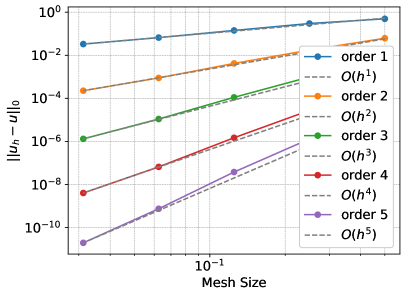
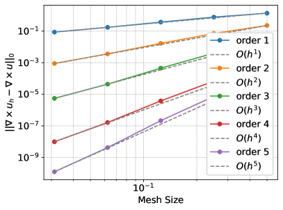
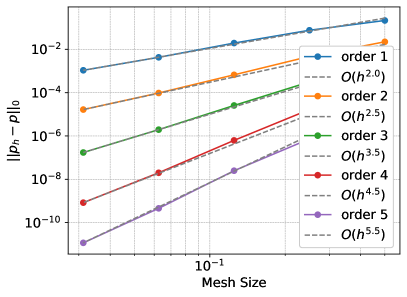
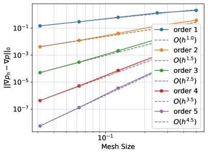
Figure 1: Convergence analysis of (top) $u$ in the $L^{2}$ and $\mathbf{H}(\operatorname{curl},\Omega)$ norms, and (bottom) $p$ in the $L^{2}$ and $H^{1}$ norms for the experiment as discussed in Section 5.1. The results for lowest-order elements are labeled as “order 1”.

5.2 Fully-driven flow on an annulus

In this second test case, we consider an annulus with inner radius of 1 and outer radius of 4 (see Figure 2). On the inner boundary we impose Dirichlet boundary conditions $\mathbf{u}=[-y,x]$. On the outer boundary, we impose a Navier slip boundary condition. This test is of particular interest as it indicates whether the scheme satisfies the objectivity criteria from [25, Sect. 6.4, Test 3]. The objectivity criteria dictate that the true solution is a rigid body motion in this example. We used 3rd order polynomials on an unstructured, curved mesh with mesh-width $h=0.25$. As shown in Figure 2, we observe that the numerical solution correctly represents a rigid body motion.

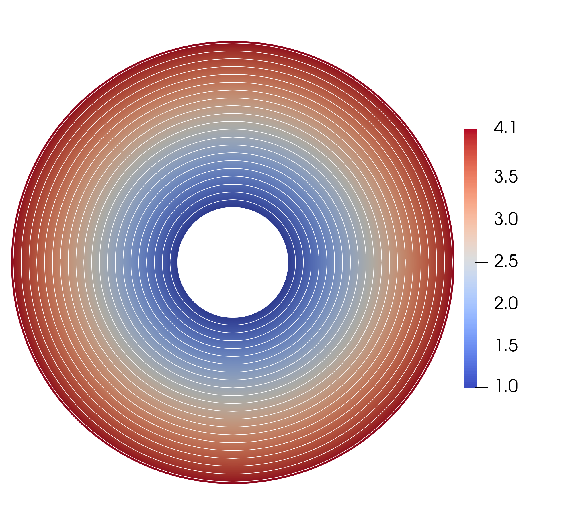
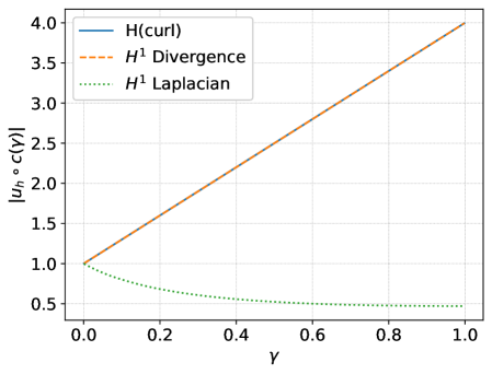
Figure 2: Visualization of the computed solution as described in Section 5.2. The “$\mathbf{H}(\operatorname{curl},\Omega)$”  method correctly produces a rigid body motion. (Left) The white lines represent the streamlines and the colors indicate the magnitude of the velocity field $\mathbf{u}$. (Right) The lines represents the magnitude of the velocity field $\mathbf{u}_{h}$ on the line segment $c(\gamma)=[1+3\gamma,0]$. Note that the blue and orange lines overlap.

5.3 Lid-driven cavity

As our third test case, we consider the lid-driven cavity. We follow [25, Sect. 6.2, Test 2] and define $\Omega$ as a unit square. We impose a Dirichlet boundary condition $\mathbf{u}=[1,0]$ on the top boundary (the “lid”) and Navier slip boundary conditions on the remaining sides. We use 3rd order polynomials on an unstructured mesh with mesh-width $h=0.05$. The results are presented in Figure 3 (Left). Since all the boundaries are straight in this case, both the “Divergence”  and the “Laplace”  formulations converge to the same solution. In Figure 3 (Right) we plot the magnitude of the approximation of the velocity field $\mathbf{u}$ on the line segment $c(\gamma)=[0.5,\gamma]$. We see that the different computed solutions agree.

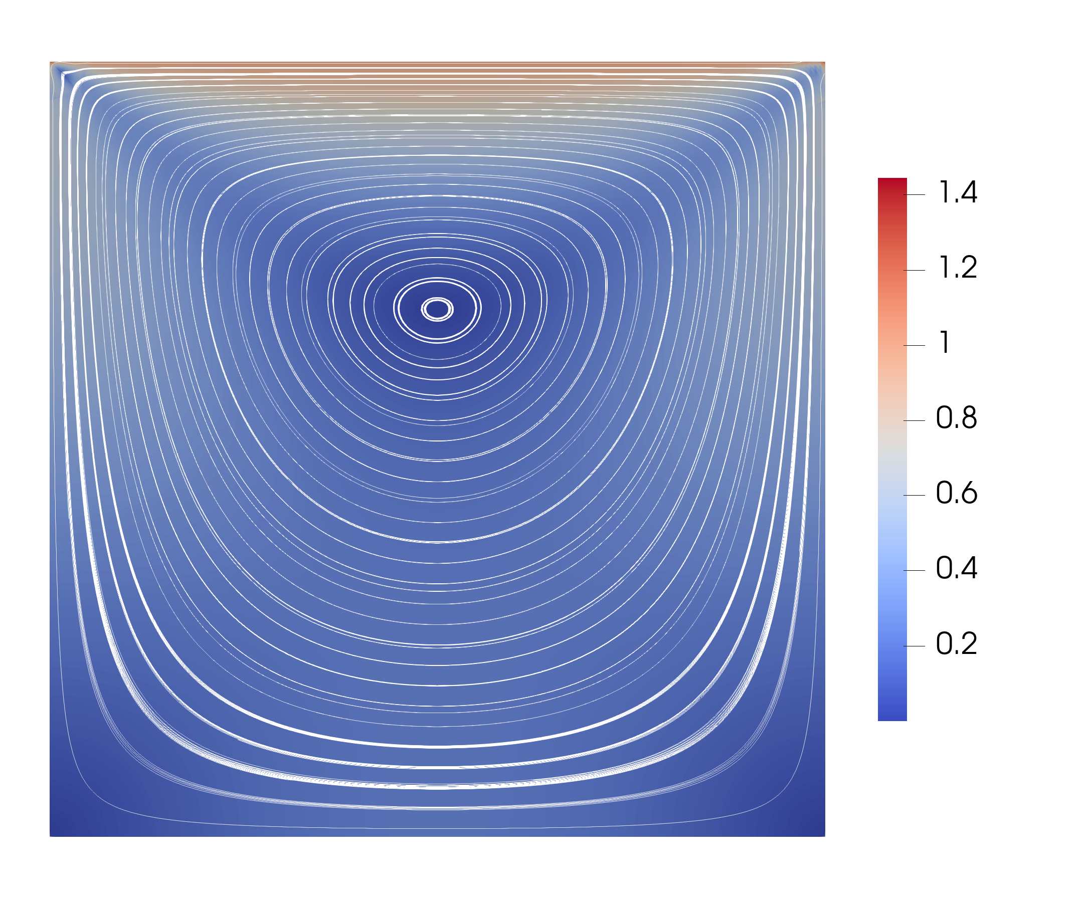
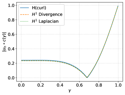
Figure 3: Visualization of the computed solution as described in Section 5.3 using 3rd order polynomials on an unstructured mesh with mesh-width $h=0.05$. The domain is a 1-by-1 square. (Left) The white lines represent the streamlines and the colors indicate the magnitude of the velocity field $\mathbf{u}$. (Right) The line represents the magnitude of the discrete velocity $\mathbf{u}_{h}$ on the line segment $c(\gamma)=[0.5,\gamma]$.

5.4 Slippery semi-circular cavity

In this experiment, we follow [25, Sect. 6.6, Test 2] and define $\Omega$ as a half-disk with radius 1 and center $(0,0)$, as illustrated in Figure 4. Again, we impose a Dirichlet boundary condition $\mathbf{u}=[1,0]$ on the top boundary and Navier slip boundary conditions on the curved part of the boundary. We used 3rd order polynomials on an unstructured, curved mesh with mesh-width $h=0.05$ and we plot the result in Figure 4 (Left). In Figure 4 (Right) we plot the $x$-component of the approximation of the velocity field $\mathbf{u}$ on the line $x=0.5$ and $y\in(0,1)$. In contrast to the test case from Section 5.3, we now observe a clear discrepancy between the “Laplace”  formulation and the other methods. Importantly, our proposed method is in close agreement with the “Divergence”  method, which corresponds to the physically accurate solution.

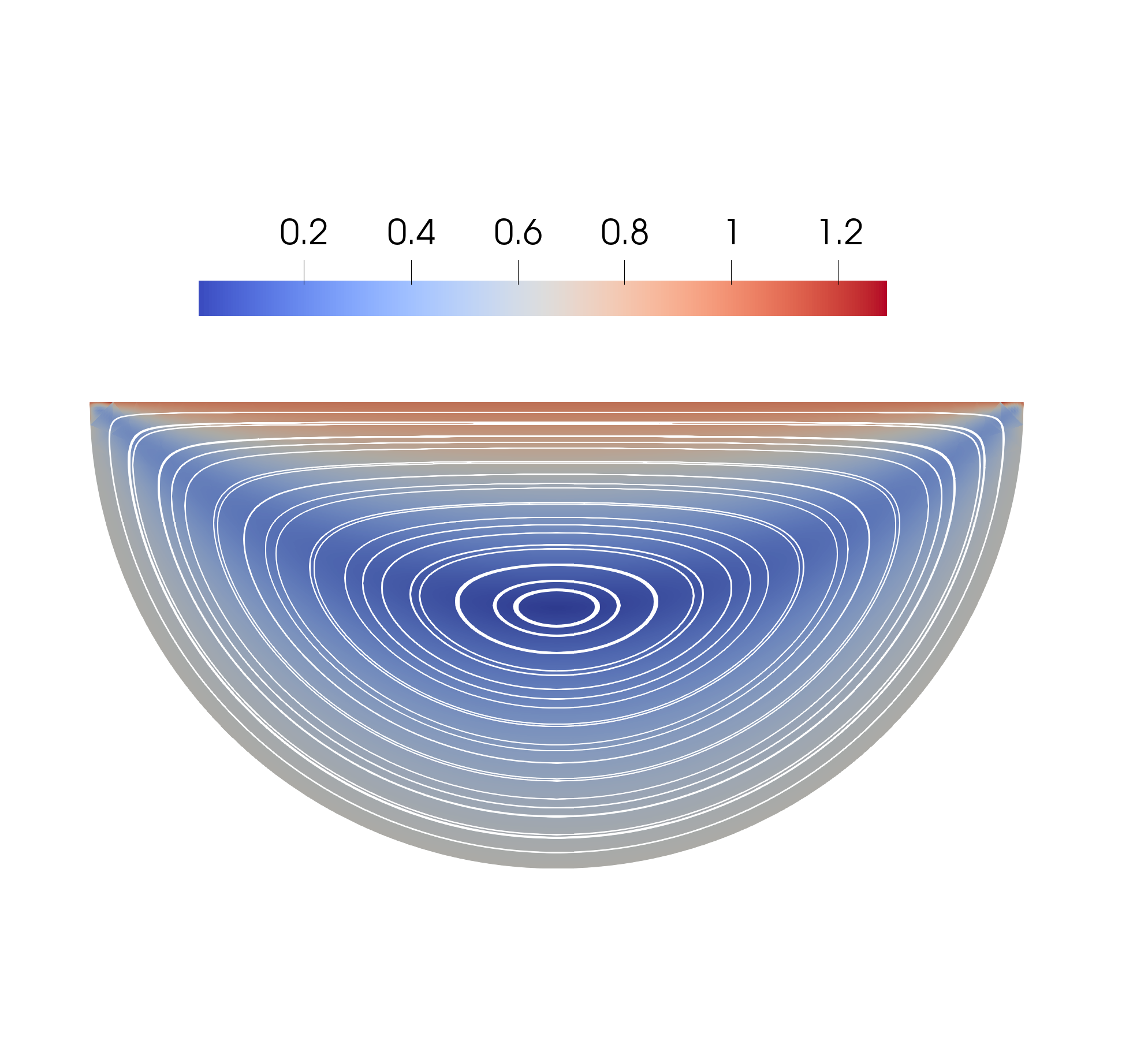
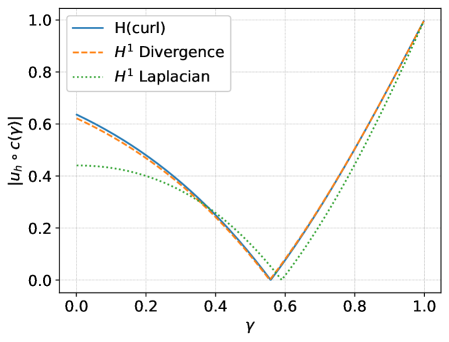
Figure 4: Visualization of the computed solution as described in Section 5.4. The domain is a half-circle of radius 1 and with center $(0,0)$. We used 3rd order polynomials on an unstructured, curved mesh with mesh-width $h=0.05$. (Left) The white lines represent the streamlines and the colors indicate the magnitude of the velocity field $\mathbf{u}_{h}$. (Right) The line represents the $x$-component of the approximation of the velocity field $\mathbf{u}$ on the line $x=0$ and $y\in(-1,0)$.

5.5 Flow around slippery cylinder

In this final experiment, we follow [25, Sect. 6.7] and let $\Omega$ be an 8-by-8 square centered at the origin, from which a circle of radius 1 is cut out, as shown in Figure 5. We impose Dirichlet boundary conditions $\mathbf{u}=[1,0]$ on the outer boundary and Navier slip boundary conditions on the curved part of the boundary. We used 3rd order polynomials on an unstructured, curved mesh with mesh-width $h=0.25$ and we plot the result in Figure 5 (Left). In Figure 5 (Right) we plot the $x$-component of the approximation of the velocity field $\mathbf{u}$ on the curve $(x,y)=(-\cos(\gamma),\sin(\gamma))$ for $\gamma\in(0,\pi)$. Again, the “$\mathbf{H}(\operatorname{curl},\Omega)$”  and “Divergence”  methods are in agreement, whereas the “Laplace”  deviates.

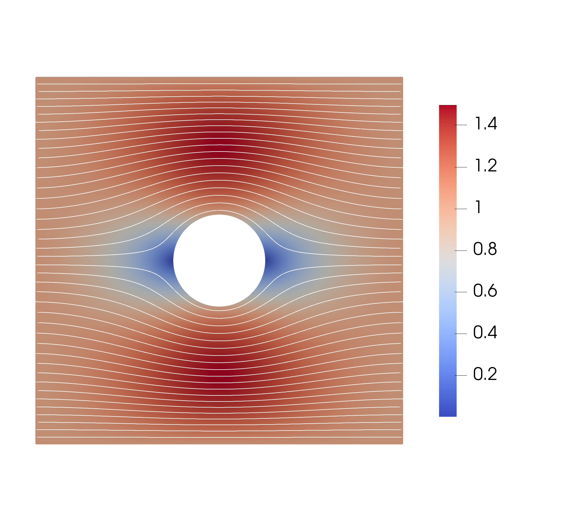
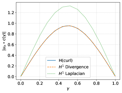
Figure 5: Visualization of the computed solution as described in Section 5.5. The domain is 8-by-8 square with a circle of radius 1 cut out at its center. We used 3rd order polynomials on an unstructured, curved mesh with mesh-width $h=0.25$. (Left) The white lines represent the streamlines and the colors indicate the magnitude of the velocity field $\mathbf{u}$. (Right) Visualization of the computed solution as described in Section 5.5. The line represents the $x$-component of the produced velocity field $\mathbf{u}_{h}$ on the the curve $(x,y)=(-\cos(\gamma),\sin(\gamma))$ for $\gamma\in(0,\pi)$.

6 Conclusions

We have considered the slip condition as a Robin condition for the Stokes equations written in rotation form. The Robin parameter is related to the Weingarten map of the boundary and since its sign may vary along the boundary, it does not necessarily form a (semi-)definite operator. Taking this into account, we showed that the system admits a solution with the velocity in the space $\mathbf{X}$ that is orthogonal to gradients.

For the analysis of the discrete problem, we considered a discrete velocity space that is only orthogonal to discrete gradients and therefore not a subspace of $\mathbf{X}$. The standard theory for conforming methods therefore did not apply and we instead employed appropriate lifting and projection operators to obtain stability and convergence estimates. These results were extended to an implementable saddle-point formulation involving the pressure.

Finally, we showcased the performance of the method through five numerical experiments. The expected convergence rates were confirmed for a family of finite element methods and we highlighted that the discrete solution exhibits physically consistent behavior.

In future work, we will consider the vorticity-velocity-pressure formulation [11] with Navier slip boundary conditions, in which the velocity is sought in $\mathbf{H}(\operatorname{div},\Omega)$. Additionally, we will analyze the imposition of Dirichlet conditions using Nitsche’s method for the Stokes equations in rotation form. Finally, we are interested in extending this work to the case of traction boundary conditions in rotation-based formulations of linearized elasticity[3, 8] (cf. Remark 2.4).

Appendix A A Nitsche-type method for Dirichlet boundary condition

Let $\Gamma=\Gamma_{\mathrm{D}}\cup\Gamma_{\mathrm{NS}}$, where $\Gamma_{\mathrm{D}}$ and $\Gamma_{\mathrm{NS}}$ denote the portions of the boundary on which Dirichlet and Navier slip boundary conditions are imposed, respectively. The bilinear form $a$ in (3.7) is then modified as follows:

$$a(\mathbf{u}_{h},\mathbf{v}_{h}) \coloneqq(\nabla\times\mathbf{u}_{h},\nabla\times\mathbf{v}_{h})+\langle\alpha\boldsymbol{\gamma}_{\parallel}(\mathbf{u}_{h}),\boldsymbol{\gamma}_{\parallel}(\mathbf{v}_{h})\rangle_{\Gamma_{\mathrm{NS}}}$$

$$+\langle\mathbf{n}\times\nabla\times\mathbf{u}_{h},\mathbf{v}_{h}\rangle_{\Gamma_{\mathrm{D}}}+\langle\mathbf{u}_{h},\mathbf{n}\times\nabla\times\mathbf{v}_{h}\rangle_{\Gamma_{\mathrm{D}}}+\frac{C_{w}}{h}\langle\mathbf{n}\times\mathbf{u}_{h},\mathbf{n}\times\mathbf{v}_{h}\rangle_{\Gamma_{\mathrm{D}}}.$$

However, analysis of this formulation falls outside the scope of this work and we will instead consider this in a subsequent paper.

References

• [1] C. Amrouche, C. Bernardi, M. Dauge, and V. Girault, Vector potentials in three-dimensional non-smooth domains, Math. Methods Appl. Sci., 21 (1998), pp. 823–864.
• [2] C. Amrouche and N. E. H. Seloula, $L^{p}$-theory for vector potentials and Sobolev’s inequalities for vector fields: application to the Stokes equations with pressure boundary conditions, Math. Models Methods Appl. Sci., 23 (2013), pp. 37–92.
• [3] V. Anaya, Z. de Wijn, D. Mora, and R. Ruiz-Baier, Mixed displacement–rotation–pressure formulations for linear elasticity, Computer Methods in Applied Mechanics and Engineering, 344 (2019), pp. 71–94.
• [4] D. N. Arnold, R. S. Falk, and J. Gopalakrishnan, Mixed finite element approximation of the vector Laplacian with Dirichlet boundary conditions, Mathematical Models and Methods in Applied Sciences, 22 (2012), p. 1250024.
• [5] D. N. Arnold, R. S. Falk, and R. Winther, Finite element exterior calculus, homological techniques, and applications, Acta Numer., 15 (2006), pp. 1–155.
• [6] D. N. Arnold and A. Logg, Periodic table of the finite elements, 2014.
• [7] W. M. Boon and A. Fumagalli, A multipoint vorticity mixed finite element method for incompressible Stokes flow, Applied Mathematics Letters, 137 (2023), p. 108498.
• [8] W. M. Boon, A. Fumagalli, and A. Scotti, Mixed and multipoint finite element methods for rotation-based poroelasticity, SIAM Journal on Numerical Analysis, 61 (2023), pp. 2485–2508.
• [9] H. Brezis, Functional analysis, Sobolev spaces and partial differential equations, Universitext, Springer, New York, 2011.
• [10] A. Buffa, M. Costabel, and D. Sheen, On traces for ${\bf H}({\bf curl},\Omega)$ in Lipschitz domains, J. Math. Anal. Appl., 276 (2002), pp. 845–867.
• [11] F. Dubois, Vorticity-velocity-pressure formulation for the Stokes problem, Math. Methods Appl. Sci., 25 (2002), pp. 1091–1119.
• [12] F. Dubois, M. Salaün, and S. Salmon, First vorticity-velocity-pressure numerical scheme for the Stokes problem, Comput. Methods Appl. Mech. Engrg., 192 (2003), pp. 4877–4907.
• [13] F. Dubois, M. Salaün, and S. Salmon, Vorticity-velocity-pressure and stream function-vorticity formulations for the Stokes problem, J. Math. Pures Appl. (9), 82 (2003), pp. 1395–1451.
• [14] R. G. Durán, Error analysis in $L^{p},\;1\leq p\leq\infty,$ for mixed finite element methods for linear and quasi-linear elliptic problems, RAIRO Modél. Math. Anal. Numér., 22 (1988), pp. 371–387.
• [15] A. Ern and J.-L. Guermond, Analysis of the edge finite element approximation of the Maxwell equations with low regularity solutions, Comput. Math. Appl., 75 (2018), pp. 918–932.
• [16]  , Finite elements I—Approximation and interpolation, vol. 72 of Texts in Applied Mathematics, Springer, Cham, [2021] ©2021.
• [17] G. N. Gatica and S. Meddahi, Finite element analysis of a time harmonic Maxwell problem with an impedance boundary condition, IMA J. Numer. Anal., 32 (2012), pp. 534–552.
• [18] V. Girault, Curl-conforming finite element methods for Navier-Stokes equations with nonstandard boundary conditions in ${\bf R}^{3}$, in The Navier-Stokes equations (Oberwolfach, 1988), vol. 1431 of Lecture Notes in Math., Springer, Berlin, 1990, pp. 201–218.
• [19] V. Girault and P.-A. Raviart, Finite element methods for Navier-Stokes equations: theory and algorithms, vol. 5, Springer Science & Business Media, 2012.
• [20] I. G. Graham, W. Hackbusch, and S. A. Sauter, Finite elements on degenerate meshes: inverse-type inequalities and applications, IMA J. Numer. Anal., 25 (2005), pp. 379–407.
• [21] M.-L. Hanot, An arbitrary order and pointwise divergence-free finite element scheme for the incompressible 3D Navier–Stokes equations, SIAM Journal on Numerical Analysis, 61 (2023), pp. 784–811.
• [22] R. Hiptmair, Finite elements in computational electromagnetism, Acta Numer., 11 (2002), pp. 237–339.
• [23] C. Johnson and V. Thomée, Error estimates for some mixed finite element methods for parabolic type problems, RAIRO Anal. Numér., 15 (1981), pp. 41–78.
• [24] R. Kress, Linear integral equations, vol. 82 of Applied Mathematical Sciences, Springer-Verlag, Berlin, 1989.
• [25] A. C. Limache, P. Sánchez, L. D. Dalcín, and S. R. Idelsohn, Objectivity tests for Navier–Stokes simulations: The revealing of non-physical solutions produced by Laplace formulations, Computer Methods in Applied Mechanics and Engineering, 197 (2008), pp. 4180–4192.
• [26] M. Mitrea and S. Monniaux, The nonlinear Hodge-Navier-Stokes equations in Lipschitz domains, Differential Integral Equations, 22 (2009), pp. 339–356.
• [27] J.-C. Nédélec, Mixed finite elements in ${\bf R}^{3}$, Numer. Math., 35 (1980), pp. 315–341.
• [28]  , Éléments finis mixtes incompressibles pour l’équation de Stokes dans $\mathbb{R}^{3}$, Numer. Math., 39 (1982), pp. 97–112.
• [29]  , A new family of mixed finite elements in ${\bf R}^{3}$, Numer. Math., 50 (1986), pp. 57–81.
• [30] M. Neunteufel, J. Schöberl, and K. Sturm, Numerical shape optimization of the Canham-Helfrich-Evans bending energy, J. Comput. Phys., 488 (2023), pp. Paper No. 112218, 26.
• [31] J. Nitsche, $L_{\infty}$-convergence of finite element approximations, in Mathematical aspects of finite element methods (Proc. Conf., Consiglio Naz. delle Ricerche (C.N.R.), Rome, 1975), vol. Vol. 606 of Lecture Notes in Math., Springer, Berlin-New York, 1977, pp. 261–274.
• [32] R. Rannacher and R. Scott, Some optimal error estimates for piecewise linear finite element approximations, Math. Comp., 38 (1982), pp. 437–445.
• [33] M. Salaün and S. Salmon, Low-order finite element method for the well-posed bidimensional Stokes problem, IMA J. Numer. Anal., 35 (2015), pp. 427–453.
• [34] S. A. Sauter and C. Schwab, Boundary element methods, vol. 39 of Springer Series in Computational Mathematics, Springer-Verlag, Berlin, 2011. Translated and expanded from the 2004 German original.
• [35] J. Schöberl, C++11 implementation of finite elements in NGSolve, Technical Report ASC-2014-30, Institute for Analysis and Scientific Computing, (2014).
• [36] W. Tonnon and R. Hiptmair, Semi-Lagrangian finite element exterior calculus for incompressible flows, Adv. Comput. Math., 50 (2024), pp. Paper No. 11, 29.
• [37] B. Yang, Robin Boundary Conditions for the Hodge Laplacian and Maxwell’s Equations, ProQuest LLC, Ann Arbor, MI, 2019. Thesis (Ph.D.)–University of Minnesota.
• [38] Y. Zhang, A. Palha, M. Gerritsma, and Q. Yao, A MEEVC discretization for two-dimensional incompressible Navier-Stokes equations with general boundary conditions, J. Comput. Phys., 510 (2024), p. Paper No. 113080.