A millisecond pulsar position determined
to 0.2 mas precision with VLBI

Abstract

Context. Precise millisecond pulsar (MSP) positions determined with very long baseline interferometry (VLBI) hold the key to building the connection between the kinematic and dynamic reference frames respectively used by VLBI and pulsar timing. The frame connection would provide an important pathway to examining the planetary ephemerides used in pulsar timing, and potentially enhancing the sensitivities of pulsar timing arrays used to detect stochastic gravitational-wave background at nano-Hz regime.

Aims. We aim at significantly improving the VLBI-based MSP position from its current $\gtrsim 1$ mas precision level by reducing the two dominant components in the positional uncertainty — the propagation-related uncertainty and the uncertainty resulting from the frequency-dependent core shifts of the reference sources.

Methods. We introduce a new differential astrometry strategy of using multiple calibrators observed at several widely separated frequencies, which we call PINPT (Phase-screen Interpolation plus frequeNcy-dePendent core shifT correction; read as ”pinpoint”) for brevity. The strategy allows determination of the core-shift and mitigates the impact of residual delay in the atmosphere. We implemented the strategy on PSR J2222$-$0137, an MSP well constrained astrometrically with VLBI and pulsar timing.

Results. Using the PINPT strategy, we determined core shifts for 4 AGNs around PSR J2222$-$0137, and derived a VLBI-based pulsar position with uncertainty of 0.17 mas and 0.32 mas in right ascension and declination, respectively, approaching the uncertainty level of the best-determined timing-based MSP positions. Additionally, incorporating the new observations into historical ones, we refined the pulsar proper motion and the parallax-based distance to the $\lesssim 10$ $\mu\mathrm{as\leavevmode\nobreak\ yr^{-1}}$ level and the sub-pc level, respectively.

Conclusions. The realization of the PINPT strategy promises a factor-of-5 positional precision enhancement (over conventional VLBI astrometry) for all kinds of compact radio sources observed at $\lesssim 2$ GHz, including most fast radio bursts.

1 Introduction

Millisecond pulsars (MSPs) refer to recycled fast-spinning neutron stars, which exhibit unparalleled spin stability compared to other pulsars (Hobbs et al., 2010). Using the pulsar timing technique (e.g. Detweiler, 1979) that time and model the pulse arrival times, astronomers have delivered the most stringent tests of gravitational theories with MSPs (e.g. Kramer et al., 2021). Collectively, an array of MSPs scattered across the sky, as known as a pulsar timing array (PTA), can be used to directly probe the stochastic gravitational-wave background (GWB) at the nHz regime (Sazhin, 1978).

Recent years have seen the major PTA consortia closing in on achieving high-significance detections of a homogeneous GWB (Agazie et al., 2023; Reardon et al., 2023; Antoniadis et al., 2023; Xu et al., 2023). Despite the breakthrough, to deepen our understanding of the sources of the GWB still requires continuous improvement of the PTA sensitivities. The optimal strategy to sustain PTA sensitivity enhancement is to regularly add new MSPs to the PTAs (Siemens et al., 2013), as has been adopted by the MPTA (Miles et al., 2023). However, it is generally difficult to quantify the red timing “noises” (in which the GWB signal resides) for a shortly timed ($\lesssim 3000$ days) MSP; one way to overcome this difficulty is to incorporate independent astrometric measurements (i.e., sky position, proper motion and parallax) into the inference of timing parameters (Madison et al., 2013).

The very long baseline interferometry (VLBI) technique can provide precise, robust and model-independent astrometric measurements for MSPs, and takes much shorter time to achieve a certain astrometric precision, as compared to the astrometric determination made with pulsar timing (e.g. Brisken et al., 2002; Chatterjee et al., 2009; Deller et al., 2019). Therefore, incorporating precise VLBI astrometric measurements into timing analysis of MSPs plays an essential role in testing gravitational theories (e.g. Deller et al., 2008; Kramer et al., 2021), and may substantially enhance the PTA sensitivities (Madison et al., 2013).

However, the incorporation is technically challenging. Firstly, incorporating precise VLBI proper motion and parallax into timing analysis can be limited by potential temporal structure evolution of the reference sources used in VLBI astrometry. Secondly, incorporating a VLBI pulsar position into timing analysis hinges on a good understanding of the transformation between the two distinct kinds of reference systems used by VLBI astrometry and pulsar timing. Though both VLBI astrometry and pulsar timing are usually presented with respect to the barycenter of the solar system, VLBI astrometry is conducted in the kinematic reference frame established with remote AGNs quasi-static on the sky (hence being robust to inaccurate planetary ephemerides), while pulsar timing studies are carried out in the dynamic reference frame that requires reliable planetary ephemerides to convert Earth-based pulse arrival times to the barycenter of the solar system. The dynamic coordinate is anchored to a kinematic coordinate system through observations of common objects, for instance, differential observations of asteroids with respect to stars. VLBI observations of MSPs with respect to AGNs will allow us to determine a rotation of the dynamic coordinate system defined by planetary ephemerides with respect to the inertial coordinate system (based on VLBI observations of AGNs) with an accuracy of 0.1 mas (Madison et al., 2013; Wang et al., 2017; Liu et al., 2023).

The residuals in pulsar positions from VLBI and timing observations after a subtraction of the rotation will allow us to provide an independent assessment of pulsar timing errors and validate the PTA error model. We consider that question as a matter of great importance because a claim that a PTA has detected GWB is based upon a model of pulsar timing errors.

So far, planetary-ephemeris-dependent frame rotation remains poorly constrained, mainly limited by relatively large ($\gtrsim 1$ mas) VLBI position uncertainties of MSPs (e.g. Liu et al., 2023), as compared to the $\lesssim 0.2$ mas timing position uncertainties for the best-timed MSPs (e.g. Perera et al., 2019). Therefore, to reduce the VLBI position uncertainties of MSPs holds the key to building the planetary-ephemeris-dependent frame tie, examining the quality of planetary ephemerides, and hence facilitating the quantification of the timing noises resulting from inaccurate planetary ephemerides. In this paper, we introduced and tested a novel method to significantly improve the precision of pulsar VLBI positions. Throughout the paper, uncertainties are provided at 68% confidence, unless otherwise stated; mathematical expressions (including the subscripts and superscripts) defined anywhere are universally valid.

2 A novel observing strategy & test observations

2.1 The PINPT strategy

As radio pulsars are generally faint ($sim1$ mJy at 1.4 GHz, and with steep spectra), the standard approach for directly determining positions in the quasi-inertial VLBI frame involving the measurement of group delays is not feasible. Instead, pulsar absolute positions have been determined using differential astrometry with respect to relatively bright reference sources, which are normally AGNs that are not point-like. Since the position of a suitable nearby AGN can be determined using standard absolute astrometry techniques, such relative position measurements allow a connection of the pulsar position into the quasi-inertial frame. However, standard absolute astrometry techniques do not account for any structure in the AGN, and so the position extracted for these sources is effectively that of the peak brightness in the image. The brightest spot in the 2D brightness distribution (or simply image) of an AGN also serves as the reference point of differential astrometry, which is usually the optically thick jet core (as long as the AGN is not flaring). As the AGN images normally vary with observing frequency $\nu$, the reference point (or the jet core) evolves with $\nu$ as well; additionally, frequency-dependent image models of the reference sources are required for pulsar astrometry.

Three main error sources contribute to the error budget of the absolute pulsar position (see Section 3.2 of Ding et al., 2020a): i) the uncertainty in the absolute position of the primary phase calibrator (derived and registered in the Radio Fundamental Catalogue, or the ICRF3 catalogue, Charlot et al., 2020), ii) the unknown frequency-dependent core shifts (hereafter simply referred to as core shifts) (e.g. Bartel et al., 1986; Lobanov, 1998) of the reference sources (or more generally, the frequency evolution of reference source structures), and iii) differences in the line of sight propagation delay between the direction of the calibrator source (where it has been solved) and the direction of the target. At L band, core shifts amounting to $\sim 1.2$ mas (Sokolovsky et al., 2011) usually dominate the error budget. Second to that, the propagation-related systematic error of the absolute pulsar position is also prominent, given the relatively large ($\gtrsim 1$ deg) separation between the pulsar and its primary phase calibrator.

To suppress the aforementioned positional uncertainties, we designed a special observing strategy of differential astrometry, which extends the core-shift-determining method pioneered by Voitsik et al. (2018), and combines the method with the Multi-View (referring specifically to 2D interpolation throughout this paper) strategy (e.g. Rioja et al., 2017; Hyland et al., 2023). The proposed observing strategy, referred to as the PINPT (Phase-screen Interpolation plus frequeNcy-dePendent core shifT correction; read as ”pinpoint”) strategy, requires a group of $\lesssim 6$ observations for absolute position determination: $\lesssim 3$ L-band Multi-View observations of the pulsar (pulsar sessions), and $\lesssim 3$ core-shift-determining observations on nearby AGNs (that include the 3 calibrators used in the Multi-View session), each at different observing frequency $\nu$. Where suitable L-band in-beam calibrators are identified, the pulsar sessions can also be used as the L-band core-shift-determining session, hence reducing the required observing time.

Our observing strategy of multi-frequency observations with multiple phase calibrators has three advantages. Firstly, with the multi-frequency observations of AGNs, the core shifts of the AGNs would be well determined, which would significantly reduce the core-shift-related errors of the absolute pulsar position. Secondly, the use of Multi-View strategy would remove propagation-related systematic errors to at least the first order (e.g. Ding et al., 2020b). Finally, with three phase calibrators of the Multi-View setup, the pulsar position uncertainties due to uncertain reference source positions would drop by a factor of $\leq\sqrt{3}$ (see Section 4.4 of Ding et al., 2020b), compared to using only one phase calibrator.

2.2 Observations

To test the PINPT strategy, we ran four observing sessions in December 2021 and January 2022 using the Very Long Baseline Array (VLBA) on PSR J2222$-$0137, a millisecond pulsar well determined astrometrically by previous campaigns (Deller et al., 2013; Guo et al., 2021, hereafter referred to as D13 and G21). The observations, carried out under the project code BD244, include two 2-hr L-band Multi-View observations and two other 2-hr core-shift-determining observations at S/X band and Ku ($\sim 15$ GHz) band, respectively. The first L-band observation was scheduled within 2 days of the S/X- and Ku-band observations (in order to minimize structure evolution of the phase calibrators), and served as both pulsar session and core-shift-determining session, whereas the second L-band observation was solely a pulsar session.

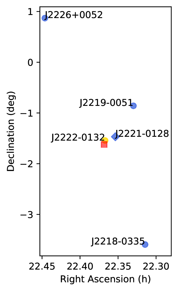
Figure 2: The calibrator plans for the observations at L, S/X and Ku bands. Each 5-min cycle of the L-band observations visited three off-beam calibrators (i.e., ICRF J221852.0$-$033536, ICRF J221947.2$-$005132, and ICRF J222646.5$+$005211), two L-band in-beam calibrators (i.e., FIRST J222112$-$012806 and FIRST J222201$-$013236) identified by Deller et al. (2013), and PSR J2222$-$0137. Accordingly, at L band, multiple combinations of calibrators can be used for the phase calibration of PSR J2222$-$0137. For enhancing the proper motion and parallax measurements of PSR J2222$-$0137, we ultimately phase-referenced PSR J2222$-$0137 to FIRST J222201$-$013236 (marked by golden circle) that was used in previous astrometric campaigns (Deller et al. 2013; Guo et al. 2021). For determining the absolute position of PSR J2222$-$0137, we applied the Multi-View strategy with the off-beam calibrators (marked by blue circles). All BD244 observations were used for core shift determination, using FIRST J222112$-$012806 (marked by blue diamond) and the off-beam calibrators. In the two sessions at S/X and Ku bands, the four AGNs marked in blue were included, while PSR J2222$-$0137 and FIRST J222201$-$013236 were skipped.

More specifically, in the L-band observations, a “target pointing” covers PSR J2222$-$0137 and two in-beam (at L band) calibrators identified by D13, i.e., FIRST J222112$-$012806 (J2221) and FIRST J222201$-$013236 (J2222); scans on this field were interleaved with scans on three brighter but off-beam AGNs (hereafter referred to as off-beam calibrators), i.e., ICRF J221852.0$-$033536 (J2218), ICRF J221947.2$-$005132 (J2219), and ICRF J222646.5$+$005211 (J2226), with a cycle time of 5 minutes. In the S/X- and Ku-band observations, J2221 and the three off-beam calibrators (hereafter referred to as the core-shift-probing AGNs) were observed alternately (by 5-min and 2-min cycles, respectively). All of the 4 core-shift-probing AGNs are selected to have displayed resolved jet-core radio features in VLBI data, which eases the core shift determination (see Section 4.2.2). Being fainter at higher observing frequencies, PSR J2222$-$0137 was skipped in the S/X- and Ku-band observations. The calibrator plans of the observations are displayed in Figure 2. In addition to the phase calibrators relatively close to PSR J2222$-$0137 on the sky, the bright blazar ICRF J214805.4$+$065738, further away from the sky region of interest, was used as the fringe finder to correct instrumental delays and filter bandpass. The unresolved flux densities and the angular separations of the aforementioned sources can be found in Table 3.

To precisely determine the core shifts, a wide variety of observing frequencies are required. The S/X-band observation simultaneously covers two frequency bands, i.e., at around $\sim 2.3$ GHz and $\sim 8.4$ GHz. Additionally, the L-band observations were designed to cover two separate frequency ranges centered around 1.44 GHz and 1.76 GHz, respectively. Altogether, we sampled 5 distinct frequency ranges, for the purpose of core shift determination. The VLBA data prior to data reduction can be accessed with the project code BD244 at https://data.nrao.edu/portal.

3 Data reduction & Direct results

All data reduction was performed with the psrvlbireduce pipeline, which runs functions of AIPS (Greisen, 2003) through ParselTongue (Kettenis et al., 2006), and images sources with DIFMAP (Shepherd et al., 1994). Despite the total observing time of only 8 hours, the data reduction of this work is sophisticated. There are two different procedures of data reduction, which depend on the purpose of the session, i.e., whether it is target session or core-shift-determining session. As noted in Section 2.2, the first L-band observation serves as both target session and core-shift-determining session, therefore being reduced twice in two distinct procedures.

3.1 Target sessions

For the data reduction of target sessions, we did not split the data by observing frequency into two (one at around 1.44 GHz and the other at around 1.76 GHz). By doing so, the average central frequency 1.6 GHz agrees with previous astrometric campaigns of PSR J2222$-$0137 (D13, G21), and the acquired image S/N (and hence the positional precision) is not lowered. As mentioned in Section 2.2, the two L-band observations involve 5 phase calibrators, including off-beam calibrators and two in-beam calibrators (also see Figure 2 and Table 3). We implemented the phase calibration of PSR J2222$-$0137 in two different ways, depending on the astrometric goal.

3.1.1 In-beam astrometry

Previous astrometric campaign of PSR J2222$-$0137 was carried out between October 2010 and June 2012, spanning 1.7 yr (D13, G21). The two new target sessions extend the astrometric time baseline by a factor of 6.6 to 11.3 yr, promising higher astrometric precision (especially for proper motion). To capitalize on the long time baseline, we phase-referenced PSR J2222$-$0137 to the same reference source (i.e., J2222) used in the previous campaign, following the data reduction procedure of D13 (including using the same image model of J2222). The updated results of in-beam astrometry is reported in Section 4.1.

3.1.2 Multi-View (2D interpolation)

As one form of the Multi-View strategy, 2D interpolation uses $\geq 3$ reference sources to derive the phase solution at the sky position of the target (e.g. Rioja et al., 2017), which can at least remove propagation-related systematic errors to the first order. In order to determine precise absolute position of PSR J2222$-$0137, we applied Multi-View (as part of the PINPT strategy) with the off-beam calibrators, all of which have well determined absolute positions¹. We reiterate that realizing the PINPT strategy requires a combination of Multi-View session(s) and core-shift-determining session(s); the two kinds of sessions need to be arranged close to each other to minimize the effects of structure evolution. The second L-band observation is $\approx 40$ days apart from the core-shift-determining sessions. Therefore, Multi-View was applied to only the first L-band observation, but not the second one.

In practice, we realized the Multi-View in two different approaches described in Appendix B. Both approaches consistently render the position $22^{\mathrm{h}}22^{\mathrm{m}}05\aas@@fstack{s}99997\!\pm\!0.1\,\mathrm{mas}$, $-01\degr 37^{\prime}15\aas@@fstack{\prime\prime}7825\!\pm\!0.2\,\mathrm{mas}$ for PSR J2222$-$0137, and $22^{\mathrm{h}}22^{\mathrm{m}}01\aas@@fstack{s}373131\!\pm\!0.03\,\mathrm{mas}$, $-01\degr 32^{\prime}36\aas@@fstack{\prime\prime}97654\!\pm\!0.06\,\mathrm{mas}$ for J2222. For further examination, we also applied the two approaches of Multi-View to the X-band data (where the chance of phase wrap errors is much smaller than at L band), and confirmed with J2221 that the two approaches give almost identical positions. The availability of the J2222 position, as well as the J2221 position $22^{\mathrm{h}}21^{\mathrm{m}}12\aas@@fstack{s}680887\!\pm\!0.01\,\mathrm{mas}$, $-01\degr 28^{\prime}06\aas@@fstack{\prime\prime}30985\!\pm\!0.02\,\mathrm{mas}$, offers a distinct pathway to the absolute position of PSR J2222$-$0137 (see Section 5). We note that the three positions presented above can only be considered relative positions with respect to the off-beam calibrators; and the positional uncertainties only include the statistical component.

3.2 Core-shift-determining sessions

The determination of AGN core shifts requires a wide coverage of observing frequencies. As mentioned in Section 2.2, the core-shift-determining sessions cover 5 frequency ranges. We first split the S/X-band data into S-band data and X-band data, and likewise split the wide-L-band data into two datasets — one at $\sim 1.44$ GHz and the other at $\sim 1.76$ GHz. Thereby, we acquired altogether 5 datasets taken at 5 different observing wavelengths $\lambda$ — 2 cm, 4 cm, 13 cm, 17 cm and 21 cm.

From each of the 5 datasets, we measured the J2221 position with respect to each off-beam calibrator by 1) phase-referencing J2221 to each off-beam calibrator, and 2) dividing the phase-referenced J2221 data by its final image model obtained at $\lambda$, and 3) fitting the J2221 position. In phase referencing, the final image model of an off-beam calibrator at $\lambda$ was applied to the phase calibration of the off-beam calibrator; subsequently, the acquired phase solution was applied to both the off-beam calibrator and J2221. To make the final image models of the off-beam calibrators and J2221, we first applied 13 cm models to the datasets of respective sources at all $\lambda$ during phase calibration (or self-calibration for J2221). In this way, we aligned the reference points of each core-shift-probing AGN across $\lambda$. Thereafter, we split out the aligned datasets, and remade the models of J2221 and off-beam calibrators at each $\lambda$. The final image models of in-beam and off-beam calibrators at all $\lambda$ were made publicly available, to convenience the reproduction of our results.

4 Astrometric parameters & Core shifts

The data reduction described in Section 3 produced a) two pulsar positions measured with respect to J2222, b) Multi-View positions of the pulsar, J2221, and J2222, and c) $5\times 3=15$ J2221 positions from the core-shift-determining sessions. The products a) and c) can provide stringent constraints on astrometric parameters and core shifts, respectively.

4.1 Astrometric inference

We added the two new pulsar positions measured with respect to J2222 to previous pulsar positions (measured with respect to J2222), and re-made the Bayesian inference as described in G21. The resultant astrometric parameters are provided in Table 1. For comparison, the previous VLBI results reported by G21 are reproduced to Table 1. Unsurprisingly, the proper motion improves substantially by a factor of $\sim 7$, while the parallax also being enhanced by $\approx 14$%, corresponding to a refined trigonometric distance of $268.6^{+1.0}_{-0.9}$ pc for PSR J2222$-$0137. On the other hand, the $3\,\sigma$ discrepancy in $\mu_{\delta}$ reveals under-estimated systematic uncertainty in declination in previous works, likely due to vertical structure evolution of J2222, which has much larger impact on short ($\lesssim 2$ yr) timespan.

Table 1: Enhanced astrometric results of PSR J2222$-$0137.

$\mu_{\alpha}$	$\mu_{\delta}$	$\varpi$	$\Omega_{\mathrm{asc}}$	$i$	Reference
($\mathrm{mas\leavevmode\nobreak\ yr^{-1}}$)	($\mathrm{mas\leavevmode\nobreak\ yr^{-1}}$)	(mas)	(deg)	(deg)	—
44.707(5)	$-5.403(12)$	$3.723^{+0.013}_{-0.014}$	190(7)	85.28(9)	this work
44.70(4)	$-5.69(8)$	$3.730^{+0.015}_{-0.016}$	$189^{+19}_{-18}$	85.25(25)	G21

4.2 Core shift determination

Following the pioneering work by Voitsik et al. (2018), we developed new packages to infer the core shifts of the 4 core-shift-probing AGNs, from the 15 J2221 positions (with respect to three off-beam calibrators at five $\lambda$) in a Bayesian style. The core shift inference requires three ingredients — (1) a prescription of systematic errors of the 15 J2221 positions, (2) mathematical description of the core shifts, and (3) an underlying mathematical relation between core shift and $\lambda$ (or observing frequency $\nu$). The three ingredients are addressed as follows.

4.2.1 Systematic errors on measured J2221 positions

Along with the 15 J2221 positions, their random errors due to noise in the J2221 images were also obtained with data reduction (described in Section 3.2). Additionally, atmospheric propagation effects would introduce systematic errors, which change with $\nu$ and the angular separation between J2221 and the reference source. We approached the systematic errors by

$$\frac{\sigma^{\mathcal{S}}_{ijk}}{1\,\mathrm{mas}}=\eta_{\mathrm{EFAC}}\cdot\eta_{0}\cdot\frac{s_{i}}{1\,\mathrm{deg}}\cdot\hat{l}(\epsilon)\cdot\frac{\sigma_{0}(\nu_{j})}{1\,\mathrm{mas}}\cdot\hat{\Theta}_{k}\,\,,$$ (1)

where $\sigma^{\mathcal{S}}_{ijk}$ denote systematic errors; the subscript $i=\mathrm{J2218,J2219,J2226}$ specifies the reference source; the second subscript $j=1,2,3,4,5$ corresponds to one of the five observing frequencies (see Section 3.2); the last subscript $k=\alpha,\delta$ refers to right ascension (RA) or declination; $\eta_{\mathrm{EFAC}}$ is a scaling factor (for the estimated systematic uncertainty) to be determined with Bayesian analysis; $\eta_{0}$ is the initial scaling factor that brings $\sigma^{\mathcal{S}}_{ijk}$ to a reasonable value ($\sim 1$ mas) before inferring $\eta_{\mathrm{EFAC}}$, which eases the inference of $\eta_{\mathrm{EFAC}}$ at a later stage; $s_{i}$ represents the angular separation between J2221 and the reference source; $\hat{\Theta}_{k}$ denotes the fractional synthesized beam size (projected to RA or declination); $\hat{l}$ and $\sigma_{0}$ stand for the two terms changing with antenna elevations $\epsilon$ and $\nu$, respectively. In this work, we set $\eta_{0}\equiv 1$; the adopted $\hat{l}(\epsilon)$ and $\sigma_{0}(\nu)$ are described in Appendix C.

4.2.2 The directions of core shifts

Regarding the ingredient (2), we describe the core shift of the $i^{\prime}$-th ($i^{\prime}=\mathrm{J2218},\mathrm{J2219},\mathrm{J2221},\mathrm{J2226}$) AGN with two parameters — the core shift magnitude $r_{i^{\prime}}$, and the direction of core shift $\theta_{i^{\prime}}$. As noted in Voitsik et al. (2018), it is difficult to infer both $r_{i^{\prime}}$ and $\theta_{i^{\prime}}$ for each of the 4 core-shift-probing AGNs from the 15 J2221 positions without prior constraints, which has been taken into account in design of the observations. As mentioned in Section 2.2, all of the core-shift-probing AGNs are selected to have displayed clear jet-core radio feature on VLBI scales. Following Voitsik et al. (2018), we assumed core shift directions are aligned with respective AGN jet directions, thereby gaining prior knowledge of the core shift directions with analysis of VLBI images of the AGNs. The determination of AGN jet directions is detailed in Appendix D.

4.2.3 The relation between core shift and observing frequency

The relation between core shift and observing frequency is given by Konigl (1981) as $r\propto\nu^{-1/k_{r}}$, where the index $k_{r}$ equals to 1 when synchrotron self-absorption (that leads to the jet core radio emissions) is in equipartition (Blandford & Königl, 1979). For the $i^{\prime}$-th AGN, we initially adopted an equivalent formalism

$$r_{i^{\prime}}=r_{0i^{\prime}}\left(\frac{\nu}{\nu_{0}}\right)^{-\beta_{i^{\prime}}}$$ (2)

as the relation between $r_{i^{\prime}}$ and $\nu$, where $\beta_{i^{\prime}}$ is a power index to be determined in Bayesian analysis; $v_{0}$ and $r_{0i^{\prime}}$ refer to the reference frequency and the core shift magnitude at the reference frequency, respectively.

Using the Bayesian inference described in Appendix E, we derive $\beta_{i^{\prime}}$ along with other model parameters. The results are provided in Table 5. When $\beta_{i^{\prime}}$ are included in the inference, the reduced chi-square $\chi^{2}_{\nu}$ of inference is 1.9. Although $\beta_{i^{\prime}}$ is significantly ($\gtrsim 3\,\sigma$) determined for 2 of the 4 AGNs, it is consistent with 1 in all cases. In comparison, when performing the inference with all $\beta_{i^{\prime}}$ fixed to 1, we acquired consistent results with generally higher precision. Moreover, the $\chi^{2}_{\nu}$ decreases to 1.2, suggesting $\beta_{i^{\prime}}\equiv 1$ as an appropriate assumption for this work. We adopt the results derived assuming $\beta_{i^{\prime}}\equiv 1$ for further analysis. The adopted core shift model is illustrated in Figure 1.

Figure 1: The jet core relative positions of FIRST J222112$-$012806 measured with respect to the jet cores of three reference sources (i.e., ICRF J221852.0$-$033536, ICRF J221947.2$-$005132, and ICRF J222646.5$+$005211) at five observing wavelengths. Systematic uncertainties calculated with Equation 1 have been included in the positional uncertainties. Models of the combined core shifts are derived assuming $\beta_{i^{\prime}}\equiv 1$ with Bayesian inference (see Appendix E), and displayed with straight lines.

5 An ultra-precise MSP position obtained with VLBI

With $r_{0i^{\prime}}$ and $\theta_{i^{\prime}}$ determined for the three off-beam calibrators and J2221, we calculated the core shifts of the 4 AGNs at 1.6 GHz, and proceeded to derive the absolute position of PSR J2222$-$0137. The derivation was realized in three approaches. In the first approach, the pulsar position obtained with Multi-View (presented in Section 3.1.2) was corrected for the core-shift refinements in the assumed positions of the off-beam calibrators (as described by Equation 9 in Appendix F). We obtained the pulsar position $\alpha^{\mathcal{G}}_{1}=22^{\mathrm{h}}22^{\mathrm{m}}05\aas@@fstack{s}99993\!\pm\!0.17\,\mathrm{mas}$, $\delta^{\mathcal{G}}_{1}=-01\degr 37^{\prime}15\aas@@fstack{\prime\prime}7841\!\pm\!0.32\,\mathrm{mas}$ in the geocentric reference frame at the reference epoch $t_{\mathrm{ref}}$ of MJD 59554.0, which corresponds to $\alpha^{\mathcal{B}}_{1}=22^{\mathrm{h}}22^{\mathrm{m}}06\aas@@fstack{s}00015\!\pm\!0.17\,\mathrm{mas}$, $\delta^{\mathcal{B}}_{1}=-01\degr 37^{\prime}15\aas@@fstack{\prime\prime}7827\!\pm\!0.32\,\mathrm{mas}$ with respect to the barycenter of the solar system after removing the parallax effects. Here, the positional uncertainty is the addition-in-quadrature of the statistical uncertainty (provided in Section 3.1.2) and the $\Delta\@vec{x}_{\mathrm{target}}$ uncertainty described in Appendix F.

In the second approach, we first acquired the J2221 position $\vec{x}_{\mathrm{J2221}}$ at 1.6 GHz by correcting the X-band J2221 position (obtained with Multi-View, see Section 3.1.2) using the same process employed in the previous approach for the target source PSR J2222$-$0137. Subsequently, we reprocessed all VLBA data (including the two new pulsar sessions and the historical ones) of PSR J2222$-$0137, phase-referencing PSR J2222$-$0137 to J2221. With the position series obtained from the data reduction, we inferred the reference pulsar position $\vec{x}_{\mathrm{psr}}^{\mathrm{\,J2221}}$ (measured with respect to J2221) and its uncertainty at $t_{\mathrm{ref}}=\mathrm{MJD}\leavevmode\nobreak\ 59554.0$ (along with other astrometric parameters) using the Bayesian analysis described in Ding et al. (2023). Combining $\vec{x}_{\mathrm{J2221}}$, the image model position $\vec{x}_{\mathrm{J2221}}^{\mathrm{\,model}}$ of J2221, and $\vec{x}_{\mathrm{psr}}^{\mathrm{\,J2221}}$, the absolute position of PSR J2222$-$0137 was determined with Equation 12 to be $\alpha^{\mathcal{B}}_{2}=22^{\mathrm{h}}22^{\mathrm{m}}06\aas@@fstack{s}00015\!\pm\!0.19\,\mathrm{mas}$, $\delta^{\mathcal{B}}_{2}=-01\degr 37^{\prime}15\aas@@fstack{\prime\prime}7825\!\pm\!0.42\,\mathrm{mas}$, where the error budget of the position is detailed in Appendix F.1.

The last approach is essentially the same as the second one, except that J2222 is used instead of J2221. Accordingly, the absolute pulsar position was calculated with the J2222 position $\vec{x}_{\mathrm{J2222}}$ at 1.6 GHz, the image model position $\vec{x}_{\mathrm{J2222}}^{\mathrm{\,model}}$ of J2222, and the reference pulsar position $\vec{x}_{\mathrm{psr}}^{\mathrm{\,J2222}}$ measured with respect to J2222. We obtained $\alpha^{\mathcal{B}}_{3}=22^{\mathrm{h}}22^{\mathrm{m}}06\aas@@fstack{s}00015\!\pm\!0.14\,\mathrm{mas}$, $\delta^{\mathcal{B}}_{3}=-01\degr 37^{\prime}15\aas@@fstack{\prime\prime}7828\!\pm\!0.27\,\mathrm{mas}$.

The pulsar positions obtained with the three approaches are summarized in the upper part of Table 2. Though all the three approaches render highly consistent absolute pulsar positions, the first approach offers a snapshot (on the timescale of AGN structure evolution) localization (of PSR J2222$-$0137) independent from the previous astrometric observations of PSR J2222$-$0137, as opposed to the two other approaches (which essentially use the multi-frequency multi-source observations to perfect the position and structure of one of the in-beam calibrators, rather than the pulsar, at that snapshot in time, and then proceeds to perform standard differential astrometry using that frozen model of the astrometric reference source). Therefore, we report $\left(\alpha^{\mathcal{B}}_{1},\delta^{\mathcal{B}}_{1}\right)$ at $t_{\mathrm{ref}}=\mathrm{MJD}\leavevmode\nobreak\ 59554.0$ as the primary absolute position of PSR J2222$-$0137.

Table 2: Absolute pulsar positions with respect to the barycenter of the solar system, derived with the PINPT strategy

	$\alpha^{\mathcal{B}}$	$\delta^{\mathcal{B}}$
	$t_{\mathrm{ref}}=\mathrm{MJD}\leavevmode\nobreak\ 59554.0$ — VLBI-only
psr. appr.	$\mathbf{22^{\mathrm{h}}22^{\mathrm{m}}06\aas@@fstack{s}00015\!\pm\!0.17\,\mathrm{mas}}$	$\mathbf{-01\degr 37^{\prime}15\aas@@fstack{\prime\prime}7827\!\pm\!0.32\,\mathrm{mas}}$
J2221 appr.	$22^{\mathrm{h}}22^{\mathrm{m}}06\aas@@fstack{s}00015\!\pm\!0.19\,\mathrm{mas}$	$-01\degr 37^{\prime}15\aas@@fstack{\prime\prime}7825\!\pm\!0.42\,\mathrm{mas}$
J2222 appr.	$22^{\mathrm{h}}22^{\mathrm{m}}06\aas@@fstack{s}00015\!\pm\!0.14\,\mathrm{mas}$	$-01\degr 37^{\prime}15\aas@@fstack{\prime\prime}7828\!\pm\!0.27\,\mathrm{mas}$
	$t_{\mathrm{ref}}=\mathrm{MJD}\leavevmode\nobreak\ 55743$ — VLBI vs timing
J2221 appr.	$22^{\mathrm{h}}22^{\mathrm{m}}05\aas@@fstack{s}969005\!\pm\!0.13\,\mathrm{mas}$	$\mathbf{-01\degr 37^{\prime}15\aas@@fstack{\prime\prime}72631\!\pm\!0.24\,\mathrm{mas}}$
J2222 appr.	$\mathbf{22^{\mathrm{h}}22^{\mathrm{m}}05\aas@@fstack{s}969042\!\pm\!0.13\,\mathrm{mas}}$	$-01\degr 37^{\prime}15\aas@@fstack{\prime\prime}72646\!\pm\!0.21\,\mathrm{mas}$
DMX	$22^{\mathrm{h}}22^{\mathrm{m}}05\aas@@fstack{s}969046\!\pm\!0.18\,\mathrm{mas}$	$-01\degr 37^{\prime}15\aas@@fstack{\prime\prime}7257\!\pm\!0.5\,\mathrm{mas}$
non-DMX	$22^{\mathrm{h}}22^{\mathrm{m}}05\aas@@fstack{s}969071\!\pm\!0.06\,\mathrm{mas}$	$-01\degr 37^{\prime}15\aas@@fstack{\prime\prime}7267\!\pm\!0.1\,\mathrm{mas}$

5.1 Comparison to timing positions

A priori, we expect the position difference between the VLBI PINPT measurement, and that made by pulsar timing, to be consistent. With a sample size of 1, it is difficult to ascribe any discrepancy to one or the other of the measurement techniques, or to a systematic difference between dynamic and kinematic frames - but we can use the level of agreement to set a probabilistic upper limit on the error contribution from any of these three potential sources. The most precise published timing-based position of PSR J2222$-$0137 is reported in G21. In Table 3 of G21, three positions are provided for $t_{\mathrm{ref}}=\mathrm{MJD}\leavevmode\nobreak\ 55743$, which include one position derived assuming a proper motion determined with VLBI, and two positions derived without using any VLBI prior (hereafter referred to as timing-only positions).

To test the PINPT strategy with pulsar timing, we re-derived $\left(\alpha^{\mathcal{B}}_{2},\delta^{\mathcal{B}}_{2}\right)$ and $\left(\alpha^{\mathcal{B}}_{3},\delta^{\mathcal{B}}_{3}\right)$ at $t_{\mathrm{ref}}=\mathrm{MJD}\leavevmode\nobreak\ 55743$ (same as that of G21) following the method described earlier in Section 5, under the assumption that the structures of J2221 and J2222 do not evolve with time. The results are displayed in Table 2. To minimize the correlation between the timing and VLBI positions, we only compare the VLBI positions to the two timing-only positions (of G21), which are listed in Table 2 as the “DMX” and “non-DMX” positions. Here, “DMX”, named by G21, refers to the pulsar timing model that describes DM with a piecewise constant function (Demorest et al., 2013; G21), while ”non-DMX” refers to the timing model that approximates DM variations with a cubic function (G21). The DMX and non-DMX timing positions are marginally consistent to within $2\,\sigma$ (here and hereafter, $\sigma$ refers to the addition-of-quadrature of the uncertainties of the two compared sides), with the uncertainty of the DMX position being more conservative than the non-DMX one.

On the other side of the comparison, $\delta^{\mathcal{B}}_{2}$ and $\delta^{\mathcal{B}}_{3}$ are consistent with each other. However, $\alpha^{\mathcal{B}}_{2}$ is smaller than $\alpha^{\mathcal{B}}_{3}$ at $3\,\sigma$ significance, which is associated with a $\sim 3\,\sigma$ discrepancy between the two $\mu_{\alpha}$ measured with respect to J2221 ($44.755^{+0.017}_{-0.014}$ $\mathrm{mas\leavevmode\nobreak\ yr^{-1}}$) and J2222 ($44.707\pm 0.005$ $\mathrm{mas\leavevmode\nobreak\ yr^{-1}}$, as reported in Table 1), respectively. The discrepancy between $\alpha^{\mathcal{B}}_{2}$ and $\alpha^{\mathcal{B}}_{3}$ likely indicates the violation of the assumption that the structures of J2221 and J2222 do not evolve with time. The jet direction of J2221 is almost aligned with the RA direction (see Figure 3). As noted in D13, the relatively severe structure evolution of J2221 is believed to cause 1) less precise parallax derived with respect to J2221 (as the parallax magnitude in the RA direction is $\approx 2.4$ times larger than in the declination direction), and 2) biased $\mu_{\alpha}$ determination. Specifically, the discrepancy between $\alpha^{\mathcal{B}}_{2}$ and $\alpha^{\mathcal{B}}_{3}$ (or the $\mu_{\alpha}$ discrepancy) can be explained by 0.56 mas larger (or fractionally 18% higher according to Table 5) $r_{\mathrm{J2221}}\left(1.6\,\mathrm{GHz}\right)$ at MJD 55743 compared to at MJD 59554. On the other hand, thanks to the horizontal jet of J2221, $\delta^{\mathcal{B}}_{2}$ is almost free from the impact of structure evolution (of J2221), hence being more favorable than $\delta^{\mathcal{B}}_{3}$, let alone the indication of vertical structure evolution of J2222 mentioned in Section 4.1. Therefore, we adopt $\left(\alpha^{\mathcal{B}}_{3},\delta^{\mathcal{B}}_{2}\right)$ as the absolute pulsar position at MJD 55743. A more sophisticated treatment in the future could incorporate positions in both axes from both sources, weighting them by some measure of expected reliability and taking into account the covariance between the two measurements.

When comparing $\left(\alpha^{\mathcal{B}}_{3},\delta^{\mathcal{B}}_{2}\right)$ to the two timing-only positions, we first find good consistency between $\left(\alpha^{\mathcal{B}}_{3},\delta^{\mathcal{B}}_{2}\right)$ and the DMX position, with $\alpha^{\mathcal{B}}_{3}$ and the DMX RA consistent to within $0.3\,\sigma$, and $\delta^{\mathcal{B}}_{2}$ and the DMX declination consistent to within $1.1\,\sigma$. On the other hand, despite the $1.5\,\sigma$ consistency between $\delta^{\mathcal{B}}_{2}$ and the non-DMX declination, $\alpha^{\mathcal{B}}_{3}$ is smaller than the non-DMX RA at $>3\,\sigma$ significance. It is not impossible that the $>3\,\sigma$ RA discrepancy is caused by the use of different kinds of reference systems. Therefore, we cannot yet conclude that the new PINPT results favour the DMX timing model over the non-DMX one with just one MSP.

Moreover, we reiterate that $\alpha^{\mathcal{B}}_{3}$ is subject to additional errors induced by potential horizontal structure evolution of J2222. A more robust test of the PINPT strategy with pulsar timing can be achieved by comparing $\left(\alpha^{\mathcal{B}}_{1},\delta^{\mathcal{B}}_{1}\right)$ to timing positions (based on different timing models) derived at MJD 59554, which will be part of an upcoming timing paper. Additionally, applying the PINPT strategy to just a few well timed MSPs will allow a much stronger test of the new strategy.

6 Summary

Using the PINPT strategy, we determine an MSP position to the $\sim 0.2$ mas precision with VLBI, which improves on the previous precision level by a factor of $\sim 5$ (e.g. Ding et al., 2020a; Liu et al., 2023), and is comparable with the precision level of the timing positions of the best-timed MSPs (e.g. Perera et al., 2019). According to Liu et al. (2023), applying the PINPT strategy to 50 MSPs promises $\lesssim 0.1$ mas precision for the connection between the kinematic and dynamic reference frames, $>3$ times more precise than the previous expectation. Considering that systematic errors of calibrator source positions are in a range of 0.05–0.2 mas¹ and unlikely to be improved within several decades, our strategy provides the position accuracy that approaches to a practical limit.

In general, the PINPT strategy can be used in a broader context: it can sharpen the VLBI localisation of any steep-spectrum compact radio source, which could facilitate the studies of, for example, fast radio bursts (e.g. Bhandari et al., 2023) or mergers of two neutron stars (e.g. Mooley et al., 2022). Furthermore, it is important to stress that the PINPT strategy is not only meant to enhance the precision of absolute positions, but would have fundamental impact on differential astrometry as well. Due to the variability of AGN core shifts (e.g. Plavin et al., 2019), proper motions and parallaxes measured with respect to AGNs could be potentially biased (e.g. D13, also see Section 5.1), which is believed to have driven the occasional inconsistencies between VLBI and timing proper motions for the longest timed MSPs (Ding et al., 2023). However, traditional differential astrometry with one calibrator is incapable of quantifying the variabilities in AGN core shifts, hence being subject to extra systematic errors. In the scenario of precise in-beam astrometry, variability in the core shifts of the reference sources is a leading source of systematic errors. Multi-epoch PINPT observations, on the other hand, can constrain the core shift variabilities, thus minimizing their corruption on astrometric results. As pulsar astrometry is considered, joining the core-shift-determining sessions to in-beam or Multi-View astrometry can provide accurate pulsar proper motions and parallaxes not biased by core shift variabilities, which can then be safely incorporated into pulsar timing analysis.

Appendix A Supporting materials for Section 2.2

Table 3: Unresolved flux densities & angular separations from PSR J2222$-$0137.

source	purpose	$\mathcal{S}_{\mathrm{18cm}}$	$\mathcal{S}_{\mathrm{13cm}}$	$\mathcal{S}_{\mathrm{4cm}}$	$\mathcal{S}_{\mathrm{2cm}}$	$\Delta_{\mathrm{psr}}$
name		($\mathrm{mJy\leavevmode\nobreak\ beam^{-1}}$)	($\mathrm{mJy\leavevmode\nobreak\ beam^{-1}}$)	($\mathrm{mJy\leavevmode\nobreak\ beam^{-1}}$)	($\mathrm{mJy\leavevmode\nobreak\ beam^{-1}}$)	(deg)
PSR J2222$-$0137	target	0.8	—	—	—	0
ICRF J221852.0$-$033536	phase cal. / CS det.	$1.5\times 10^{3}$	$1.0\times 10^{3}$	$1.4\times 10^{3}$	$1.8\times 10^{3}$	2.13
ICRF J221947.2$-$005132	phase cal. / CS det.	165.2	113.9	113.0	111.5	0.96
ICRF J222646.5$+$005211	phase cal. / CS det.	249.2	267.7	459.3	762.2	2.75
FIRST J222112$-$012806	phase cal. / CS det.	24.7	9.5	10.5	9.7	0.27
FIRST J222201$-$013236	phase cal.	14.5	—	—	—	0.08
ICRF J214805.4$+$065738	fringe finder	$1.5\times 10^{3}$	$1.1\times 10^{3}$	$1.5\times 10^{3}$	$2.2\times 10^{3}$	12.07

Appendix B Two approaches of Multi-View (2D interpolation)

As mentioned in Section 3.1.2, Multi-View was realized in two approaches. In both approaches, J2219 — the closest to PSR J2222$-$0137 among the off-beam calibrators, was used as the main phase calibrator. In the first approach, we made a phase calibration with J2219, then interpolated the phase solution to the approximate sky position of PSR J2222$-$0137 by performing two 1D interpolation operations (e.g. Ding et al. 2020b) one after another. Specifically, the first 1D interpolation extrapolated the phase solution to the intersection of two straight lines — one connecting J2219 and J2226, and the other connecting J2218 and J2226. Then the second 1D interpolation derived the phase solution at the position of PSR J2222$-$0137.

In the second approach, the phase solution acquired with J2219 was passed to J2218 and J2226. Subsequently, self-calibration was performed with both J2218 and J2226. The acquired incremental phase solutions $\phi_{\mathrm{J2218}}$ and $\phi_{\mathrm{J2226}}$ were then linearly added together as $c_{\mathrm{J2218}}\cdot\phi_{\mathrm{J2218}}+c_{\mathrm{J2226}}\cdot\phi_{\mathrm{J2226}}$ (here, $c_{\mathrm{J2218}}$ and $c_{\mathrm{J2226}}$ are constants described in Appendix F), which essentially moves the virtual calibrator (explained in Ding et al. 2020b) to the approximate sky position of the target (i.e., PSR J2222$-$0137, J2221, or J2222).

Appendix C $\hat{l}(\epsilon)$ and $\sigma_{0}(\nu)$

In Equation 1, there are two functions — $\hat{l}(\epsilon)$ and $\sigma_{0}(\nu)$. The former describes the fractional atmospheric path length as a function of the antenna elevation $\epsilon$, while the latter characterizes the evolution of the systematic error with respect to the observing frequency $\nu$. We define $\hat{l}(\epsilon)$ as $l/R_{\mathrm{E}}$, where $l$ and $R_{\mathrm{E}}$ are, respectively, the atmospheric path length and the radius of the Earth (not including the atmosphere). It is easy to calculate that

$$\hat{l}(\epsilon)=\overline{\sqrt{\sin^{2}{\epsilon}+2\eta_{\mathrm{H}}+{\eta_{\mathrm{H}}}^{2}}-\sin{\epsilon}}\,\,,$$ (3)

where the overline commands averaging over the observation; $\eta_{\mathrm{H}}=h_{\mathrm{atmo}}/R_{\mathrm{E}}$ is the atmosphere thickness divided by $R_{\mathrm{E}}$. We adopted $\eta_{\mathrm{H}}=0.15$ calculated with the upper height of the ionosphere ($\approx 965$ km) and the average Earth radius of 6371 km.

Using simulations, the relation between propagation-related positional error and $\nu$ has been studied by Martí-Vidal et al. (2010), and is provided in Figure 6 of Martí-Vidal et al. (2010). As the simulations of Martí-Vidal et al. (2010) assume a 5° angular separation between the target and the reference source, we divided the results of Martí-Vidal et al. (2010) by a factor of 5 (to reach the systematics per degree separation), and adopted the divided results as $\sigma_{0}(\nu)$. In Equation 1, we assume $\sigma^{\mathcal{S}}_{ijk}\propto\hat{l}(\epsilon)\cdot\sigma_{0}(\nu_{j})$, while having little knowledge about the coefficient. Therefore, the nuisance parameter $\eta_{\mathrm{EFAC}}$ (to be determined in Bayesian inference) is essential for completing Equation 1, and recovering the true magnitude of $\sigma^{\mathcal{S}}_{ijk}$.

Appendix D The determination of AGN jet directions

AGN jet directions $\phi_{\mathrm{jet}}$ and their uncertainties have been directly estimated from their VLBI images (e.g. Kovalev et al. 2017). Likewise, we determined $\phi_{\mathrm{jet}}$ of the 4 core-shift-probing AGNs from the final image models³ of the 4 sources using the newly developed package arcfits. The obtained $\phi_{\mathrm{jet}}$ results are illustrated alongside the AGN images in Figure 3, and provided in Table 4. arcfits derives $\phi_{\mathrm{jet}}$ and their uncertainties in an automatic way described as follows.

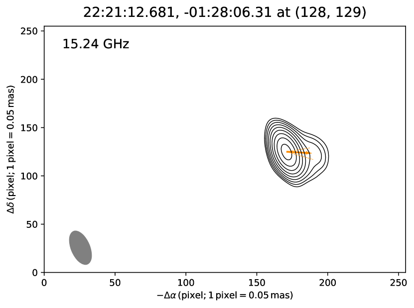
(a) FIRST J222112$-$012806

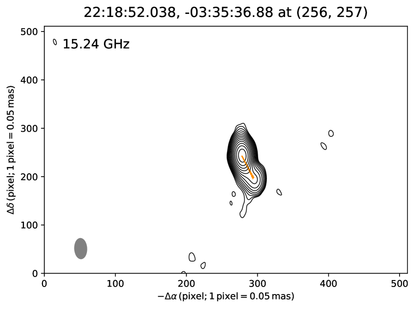
(b) ICRF J221852.0$-$033536

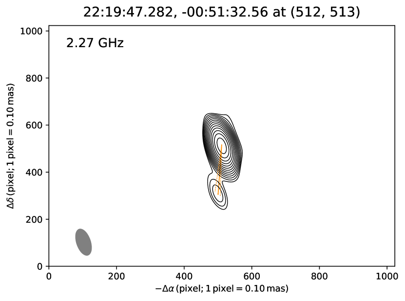
(c) ICRF J221947.2$-$005132

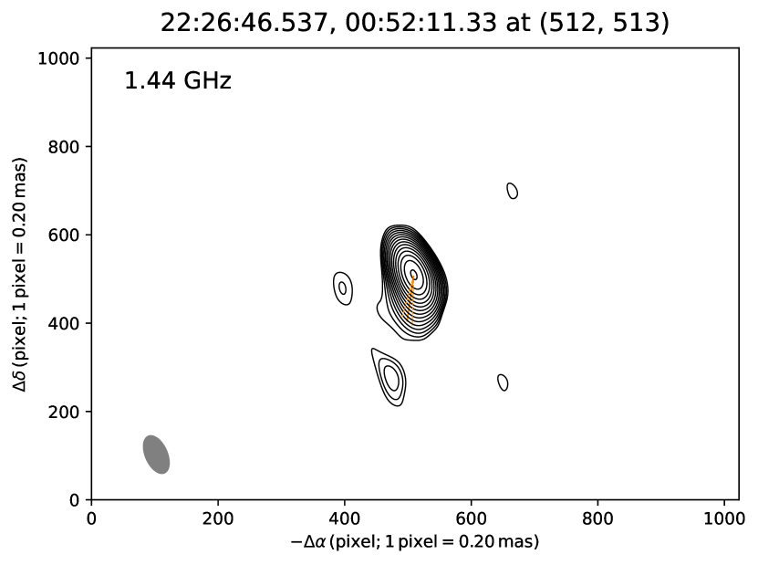
(d) ICRF J222646.5$+$005211

Figure 3: AGN contour plots obtained from the core-shift-determining sessions, and the AGN jet directions determined with arcfits. The flux density on the $m$-th ($m=1,2,3,...$) contour equals to $3\cdot\mathrm{rms}\cdot\left(\sqrt{2}\right)^{m-1}$, where rms is 0.18 $\mathrm{mJy\leavevmode\nobreak\ beam^{-1}}$, 7.3 $\mathrm{mJy\leavevmode\nobreak\ beam^{-1}}$, 0.50 $\mathrm{mJy\leavevmode\nobreak\ beam^{-1}}$ and 0.65 $\mathrm{mJy\leavevmode\nobreak\ beam^{-1}}$ for J2221, J2218, J2219 and J2226, respectively. $\Delta\alpha$ and $\Delta\delta$ are, respectively, relative right ascension (left to the east) and relative declination in the unit of image pixel. The reference position of each image is provided over the image. In each panel, the grey ellipse shows the size of the synthesized beam; the AGN jet direction is marked with the orange arrow, while the uncertainty of the direction is illustrated with the two dashed lines.

Table 4: AGN jet position angles $\phi_{\mathrm{jet}}$ determined with arcfits.

source name	$\phi_{\mathrm{jet}}$
	(deg)
ICRF J221852.0$-$033536	$220(3)$
ICRF J221947.2$-$005132	$157^{+4}_{-5}$
FIRST J222112$-$012806	$276^{+7}_{-9}$
ICRF J222646.5$+$005211	$152^{+8}_{-7}$

D.1 The noise level of the residual map

After reading a VLBI image, a 2D array of flux densities can be obtained. From this 2D map, the noise level rms of the residual map (i.e., the image after removing all detected source components) can be derived, which is a preparation for measuring $\phi_{\mathrm{jet}}$. We established the residual map and estimated the rms in the following way. We first marginalized the 2D array of flux densities into a 1D array, and calculated the standard deviation of the flux densities. All flux densities higher than 7 times the standard deviation were considered “detected”, and were removed from the 1D array. We repeated this standard deviation calculation and removal of detected points until we reached the residual map, in which no more detection can be identified. The standard deviation of this residual map was adopted as the residual map noise level rms.

D.2 Elliptical cuts on the inner regions of VLBI images

The hitherto most advanced method of measuring the position angles of radio features outside the compact radio core is by 1) converting the positions in a VLBI image from Cartesian coordinate to a polar coordinate centered around the brightest spot of the image, and 2) applying circular cuts to the VLBI image (e.g. Cui et al. 2023). As the core shift study is concerned, a $\phi_{\mathrm{jet}}$ determined close to the compact radio core is expected to better approximate the core shift direction, as compared to a $\phi_{\mathrm{jet}}$ determined afar (e.g. Konigl 1981). Due to intrinsic structure and/or scatter broadening, the compact radio core is usually larger than the synthesized beam, while normally resembling the beam (e.g., Figure 3). In other words, there is no prior information about the size of the compact radio core. As a result, when the synthesized beam is non-circular, circular cuts applied in close proximity to the compact radio core might lead to the misidentification of the compact radio core (stretching along the major axis) as radio features outside the compact core. Although this anomaly can be corrected by human intervention, other systematic errors might be introduced during the human intervention.

As a novel method that is i) largely free of human intervention, and ii) dedicated to $\phi_{\mathrm{jet}}$ determination in close proximity to the compact radio core, we cut an image model with a number of increasingly large ellipses that a) have the same axis ratio and position angle as the synthetic beam, and b) are centered at the image pixel of the highest flux density. Given that the position angle and axis ratio are both constant, the $n$-th ($n=1,2,3,...$) ellipse can be characterized by its semi-major axis $a_{n}$; a position on this ellipse can be defined with one additional parameter — the position angle (east of north) $\phi$. In this work, we universally adopted

$$a_{n}=a_{\mathrm{beam}}+(n-1)\cdot\left(a_{\mathrm{beam}}/2\right)$$ (4)

for the ellipses, where $a_{\mathrm{beam}}$ refers to the semi-major axis of the synthesized beam.

Among the ellipses ascertained by Equation 4, the innermost ellipse outside the compact radio core was used to derive $\phi_{\mathrm{jet}}$; the position angle corresponding to the maximum flux density on the ellipse was adopted as the $\phi_{\mathrm{jet}}$. An ellipse is considered outside the compact radio core, when it meets the following criteria:

1. the maximum flux density on the ellipse is $>7$ rms (see Appendix D.1 for the meaning and calculation of rms), and

2. the median flux density on the ellipse is $<3$ rms, and

3. $\phi_{\mathrm{jet}}$ uncertainty can be calculated with the method detailed in Appendix D.3.

If no ellipse meets the criteria, the AGN is considered a compact source without extended radio features.

D.3 The uncertainty on the AGN jet direction

In Appendix D.2, we adopted the position angle of the maximum flux density $\mathcal{S}_{\mathrm{max}}$ on the innermost elliptical cut outside the compact radio core as the $\phi_{\mathrm{jet}}$. Random noises in the image might distort the flux density distribution, and deviate the position of the maximum flux density on the ellipse. The degree of flux density change due to random noises is limited: the chance of large flux density changes due to random noises is lower than smaller flux density changes. Given a flux density drop $\Delta\mathcal{S}$ induced by random noises, one can estimate the chance of the drop by counting flux densities $<\bar{\mathcal{S}}_{\mathrm{R}}-\Delta\mathcal{S}$ in the residual map (see Appendix D.1 for explanation of the residual map), where $\bar{\mathcal{S}}_{\mathrm{R}}$ stands for the mean flux density of the residual map. Reversely, provided a confidence level where the flux densities in the residual map is $\geq\bar{\mathcal{S}}_{\mathrm{R}}-\Delta\mathcal{S}$, we can derive the $\Delta\mathcal{S}$ corresponding to the confidence level. In this way, we estimated $\Delta\mathcal{S}$ corresponding to 68% confidence level from the residual map. At 68% confidence, we expect $S^{\prime}_{\mathrm{max}}>S_{\mathrm{max}}-\Delta\mathcal{S}$, where $S^{\prime}_{\mathrm{max}}$ is the maximum flux density changed by random noises.

On the ellipse (where $\phi_{\mathrm{jet}}$ is determined), we identify all position angles $\phi$ where the flux densities equal to $S_{\mathrm{max}}-\Delta\mathcal{S}$. When exactly two $\phi$ are acquired, the two $\phi$ are adopted as the $1\,\sigma$ uncertainty interval of $\phi_{\mathrm{jet}}$. Otherwise (which is rare), we consider the ellipse likely still intersects the compact radio core, and move onto the next ellipse further afield.

Appendix E The Bayesian inference of core shifts

We derived the core shift model with quartet, a newly developed package dedicated to inferring core-shift-related parameters in a Bayesian manner, which is explained as follows.

E.1 Mathematical formalism

Apart from the aforementioned parameters $r_{i}$, $\theta_{i}$, $\beta_{i}$ and $\eta_{\mathrm{EFAC}}$, the reference positions $x^{*}_{ik}$ are also required in the model of core shifts. For the Bayesian inference, the likelihood function is

$$P_{\mathrm{CS}}\propto\left(\prod_{i}\prod_{j}\prod_{k}\sigma_{ijk}\right)^{-1}\exp{\left[-\frac{1}{2}\sum_{i}\sum_{j}\sum_{k}\left(\frac{x_{ijk}-\tilde{x}_{ijk}}{\sigma_{ijk}}\right)^{2}\right]}\,,$$ (5)

where $x_{ijk}$ and $\tilde{x}_{ijk}$ refer to, respectively, the observed and the modeled J2221 positions with respect to the $i$-th reference source at observing frequency $\nu_{j}$; the total positional uncertainty $\sigma_{ijk}$ is the addition-in-quadrature of random and systematic errors. In Equation 5, the modeled J2221 positions $\tilde{x}_{ijk}$ follow the relation

$$\begin{split}\tilde{x}_{ij\alpha}&=\left[r_{\mathrm{J2221}}(\nu_{j})\cos{\theta_{\mathrm{J2221}}}-r_{i}(\nu_{j})\cos{\theta_{i}}\right]+x^{*}_{i\alpha}\\ \tilde{x}_{ij\delta}&=\left[r_{\mathrm{J2221}}(\nu_{j})\sin{\theta_{\mathrm{J2221}}}-r_{i}(\nu_{j})\sin{\theta_{i}}\right]+x^{*}_{i\delta}\,,\end{split}$$ (6)

where the formalism of $r_{i^{\prime}}(\nu_{j})$ is given by Equation 2.

E.2 Priors

For the Bayesian inference, we adopted the following prior information:

1. When the inference of $\beta_{i^{\prime}}$ is requested, the prior constraints of $\beta_{i^{\prime}}$ follow a uniform distribution between 0.3 and 3, which is denoted as $\beta_{i^{\prime}}\sim\mathcal{U}\left(0.3,3\right)$.

2. $r_{0i^{\prime}}\sim\mathcal{U}\left(0,5\right)$, where the unit is mas.

3. $x^{*}_{ik}\sim\mathcal{U}\left(\overline{x_{ij}}|_{k}-3\sigma_{x_{ij}}|_{k},\,\,\overline{x_{ij}}|_{k}+3\sigma_{x_{ij}}|_{k}\right)$, where $\overline{x_{ij}}|_{k}$ and $\sigma_{x_{ij}}|_{k}$ stand for the average and standard deviation of $x_{ijk}$ at a given $k$; one lower limit and one upper limit are universally used for all reference sources.

4. $\eta_{\mathrm{EFAC}}\sim\mathcal{U}\left(0,20\right)$.

5. The prior constraints on $\theta_{i^{\prime}}$ follow Gaussian distributions characterized by the AGN jet directions $\phi_{\mathrm{jet}}$ in Table 4. Namely, $\theta_{i^{\prime}}\sim\mathcal{G}\left(\phi_{\mathrm{jet}}|_{i^{\prime}},\sigma_{\phi_{\mathrm{jet}}}|_{i^{\prime}}\right)$. In the case of asymmetric $\phi_{\mathrm{jet}}$ uncertainty, the larger side of the uncertainty is used as the $\sigma_{\phi_{\mathrm{jet}}}|_{i^{\prime}}$.

Table 5: Core shift models derived at the reference frequency of 2.27 GHz with Bayesian inference.

Model	AGN name
parameter	ICRF J221852.0$-$033536	ICRF J221947.2$-$005132	ICRF J222646.5$+$005211	FIRST J222112$-$012806
	$\beta_{i^{\prime}}$ inferred $\rightarrow\chi^{2}_{\nu}=1.9$
$\beta_{i^{\prime}}$	$0.8^{+0.3}_{-0.2}$	$1.0^{+0.9}_{-0.5}$	$1.4^{+0.8}_{-0.6}$	$0.73^{+0.22}_{-0.18}$
$r_{0i^{\prime}}$ (mas)	$3.45^{+0.33}_{-0.36}$	$0.70^{+0.34}_{-0.26}$	$2.3^{+0.5}_{-0.4}$	$2.19^{+0.32}_{-0.25}$
$\theta_{i^{\prime}}$ (deg)	$218\pm 3$	$156\pm 5$	$149^{+5}_{-6}$	$284\pm 5$
$x^{*}_{i\alpha}$	$22^{\mathrm{h}}21^{\mathrm{m}}12\aas@@fstack{s}680988\!\pm\!0.07\,\mathrm{mas}$	$22^{\mathrm{h}}21^{\mathrm{m}}12\aas@@fstack{s}681004\!\pm\!0.04\,\mathrm{mas}$	$22^{\mathrm{h}}21^{\mathrm{m}}12\aas@@fstack{s}681011\!\pm\!0.09\,\mathrm{mas}$	—
$x^{*}_{i\delta}$	$-01\degr 28^{\prime}06\aas@@fstack{\prime\prime}30895\!\pm\!0.15\,\mathrm{mas}$	$-01\degr 28^{\prime}06\aas@@fstack{\prime\prime}30891\!\pm\!0.08\,\mathrm{mas}$	$-01\degr 28^{\prime}06\aas@@fstack{\prime\prime}30852\!\pm\!0.17\,\mathrm{mas}$	—
$\eta_{\mathrm{EFAC}}$	$5.0^{+1.4}_{-1.1}$
	$\beta_{i^{\prime}}\equiv 1$ $\rightarrow\chi^{2}_{\nu}=1.2$
$r_{0i^{\prime}}$ (mas)	$3.25\pm 0.27$	$0.69^{+0.28}_{-0.29}$	$2.3\pm 0.4$	$1.98^{+0.17}_{-0.16}$
$\theta_{i^{\prime}}$ (deg)	$218\pm 3$	$157\pm 5$	$150\pm 5$	$284\pm 6$
$x^{*}_{i\alpha}$	$22^{\mathrm{h}}21^{\mathrm{m}}12\aas@@fstack{s}680989\!\pm\!0.06\,\mathrm{mas}$	$22^{\mathrm{h}}21^{\mathrm{m}}12\aas@@fstack{s}681006\!\pm\!0.03\,\mathrm{mas}$	$22^{\mathrm{h}}21^{\mathrm{m}}12\aas@@fstack{s}681011\!\pm\!0.07\,\mathrm{mas}$	—
$x^{*}_{i\delta}$	$-01\degr 28^{\prime}06\aas@@fstack{\prime\prime}30897\!\pm\!0.13\,\mathrm{mas}$	$-01\degr 28^{\prime}06\aas@@fstack{\prime\prime}30891\!\pm\!0.07\,\mathrm{mas}$	$-01\degr 28^{\prime}06\aas@@fstack{\prime\prime}30844\!\pm\!0.16\,\mathrm{mas}$	—
$\eta_{\mathrm{EFAC}}$	$4.8^{+1.4}_{-1.0}$

Appendix F The calculation of an absolute pulsar position and its uncertainty

The determination of the absolute position of PSR J2222$-$0137 through the PINPT strategy relies on well determined absolute positions of the off-beam calibrators. This work is based on the off-beam calibrator positions $\@vec{x}^{\mathrm{\,RFC}}_{i}$ reported in the 2024A release of the Radio Fundamental Catalogue¹ (RFC). Generally speaking, for Multi-View carried out with 3 off-beam calibrators, the relation between the target position $\vec{x}_{\mathrm{target}}$ and the off-beam calibrator positions $\vec{x}_{q}$ ($q=1,2,3$) is

$$\vec{x}_{\mathrm{target}}=\sum_{q}^{3}c_{q}\vec{x}_{q}\,,$$ (7)

where $\vec{x}_{\mathrm{target}}$ is known to a precision good enough to guide the Multi-View; $c_{q}$ are coefficients that can be solved with the additional condition

$$\sum_{q}^{3}c_{q}=1\,.$$ (8)

Therefore, in Multi-View, offsets in the off-beam calibrator positions would lead to offset in the target position (refined with Multi-View), as

$$\Delta\vec{x}_{\mathrm{target}}=\sum_{q}^{3}c_{q}\cdot\Delta\vec{x}_{q}\,,$$ (9)

where $\Delta\vec{x}_{q}$ result from 1) core shifts of the off-beam calibrators, and 2) inaccurate positions of the off-beam calibrator image models, and are calculated by

$$\Delta\vec{x}_{q}=\left(\@vec{x}^{\mathrm{\,model}}_{q}-\@vec{x}^{\mathrm{\,RFC}}_{q}\right)+\left[\vec{r}_{q}\left(\nu_{\mathrm{psr}}\right)-\@vec{r}_{q}^{\mathrm{\,RFC}}\right]\,.$$ (10)

Here, $\@vec{x}^{\mathrm{\,model}}_{q}$ refers to the image model position of the $q$-th off-beam calibrator; $\vec{r}_{q}\left(\nu_{\mathrm{psr}}\right)$ denotes the core shift of the $q$-th off-beam calibrator at the observing frequency of interest (which is 1.6 GHz, the observing frequency of the pulsar sessions, for this work); $\@vec{r}_{q}^{\mathrm{\,RFC}}$ is the residual core shift of the RFC position.

Specific to this work, $q=i=\mathrm{J2212},\mathrm{J2219},\mathrm{J2226}$. $c_{i}$ for various targets are provided in Table 6. According to Porcas (2009), $\@vec{r}_{i}^{\mathrm{\,RFC}}=0$, when 1) $\@vec{x}^{\mathrm{\,RFC}}_{i}$ is derived with group-delay astrometry (that removes the ionosphere-induced group delay with dual-band or multi-band geodetic observations), and 2) $\beta_{i}=1$. Both conditions are met for this work: $\@vec{x}^{\mathrm{\,RFC}}_{i}$ are estimated with group-delay astrometry; and we already assume that $\beta_{i}\equiv 1$ in the Bayesian analysis (see Section 4.2.3). Therefore, we adopt $\@vec{r}_{i}^{\mathrm{\,RFC}}=0$ in this work.

Table 6: $c_{i}$ (of Equation 7) for different targets.

Target name	$c_{\mathrm{J2218}}$	$c_{\mathrm{J2219}}$	$c_{\mathrm{J2226}}$
PSR J2222$-$0137	0.53	0.07	0.40
FIRST J222112$-$012806	0.38	0.36	0.25
FIRST J222201$-$013236	0.49	0.12	0.38

The uncertainty on $\Delta\vec{x}_{\mathrm{target}}$ is calculated by the addition-in-quadrature of the uncertainties on the components $c_{i}\Delta\@vec{x}_{i}$, where the uncertainty of $\Delta\@vec{x}_{i}$ is further derived by the addition-in-quadrature of the uncertainties on $\@vec{x}^{\mathrm{\,RFC}}_{i}$ and $\vec{r}_{i}$.

F.1 Deriving an absolute pulsar position via a nearby AGN

When the target itself is an AGN (e.g. J2221, J2222), Equation 9 needs to be generalized to

$$\Delta\vec{x}_{\mathrm{target}}=\sum_{q}^{3}c_{q}\cdot\Delta\vec{x}_{q}+\Delta\vec{r}_{\mathrm{target}}\,,$$ (11)

where $\Delta\vec{r}_{\mathrm{target}}$ is the core shift difference between $\nu_{\mathrm{psr}}$ and the observing frequency $\nu_{\mathrm{IBC}}$ of the AGN target. Accordingly, the uncertainty on $\Delta\vec{x}_{\mathrm{target}}$ is further added in quadrature by the uncertainty of $\Delta\vec{r}_{\mathrm{target}}$.

The availability of a nearby AGN (hereafter referred to as IBC) around a pulsar (or other targets of interest) provides an alternative pathway to the absolute position of the pulsar. After applying the position correction $\Delta\vec{x}_{\mathrm{target}}$ calculated with Equation 11, the absolute position $\@vec{x}_{\mathrm{IBC}}$ of the IBC at $\nu_{\mathrm{psr}}$ can be derived. Provided i) the image model position $\vec{x}_{\mathrm{IBC}}^{\mathrm{\,model}}$ of the IBC, and ii) the pulsar position $\vec{x}_{\mathrm{psr}}^{\mathrm{\,PR}}$ determined with phase referencing with respect to the IBC, the absolute pulsar position can be calculated as

$$\vec{x}_{\mathrm{psr}}=\vec{x}_{\mathrm{psr}}^{\mathrm{\,PR}}+\left(\@vec{x}_{\mathrm{IBC}}-\vec{x}_{\mathrm{IBC}}^{\mathrm{\,model}}\right)\,.$$ (12)

This pathway of deriving the absolute position may become the only option in cases where Multi-View of the target of interest cannot be arranged (e.g., when the target is an unpredictable radio transient). The uncertainty of $\vec{x}_{\mathrm{psr}}$ derived via the IBC is the addition-in-quadrature of the $\Delta\vec{x}_{\mathrm{target}}$ uncertainty, the $\vec{x}_{\mathrm{psr}}^{\mathrm{\,PR}}$ uncertainty (estimated with Bayesian inference in this work), and the statistical uncertainty of the IBC position obtained with Multi-View at $\nu_{\mathrm{IBC}}$.