Fully Test-Time rPPG Estimation via Synthetic Signal-Guided Feature Learning

Abstract

Many remote photoplethysmography (rPPG) estimation models have achieved promising performance on the training domain but often fail to measure the physiological signals or heart rates (HR) on test domains. Domain generalization (DG) or domain adaptation (DA) techniques are therefore adopted in the offline training stage to adapt the model to the unobserved or observed test domain by referring to all the available source domain data. However, in rPPG estimation problems, the adapted model usually confronts challenges of estimating target data with various domain information, such as different video capturing settings, individuals of different age ranges, or of different HR distributions. In contrast, Test-Time Adaptation (TTA), by online adapting to unlabeled target data without referring to any source data, enables the model to adaptively estimate rPPG signals of various unseen domains. In this paper, we first propose a novel TTA-rPPG benchmark, which encompasses various domain information and HR distributions, to simulate the challenges encountered in rPPG estimation. Next, we propose a novel synthetic signal-guided rPPG estimation framework with a two-fold purpose. First, we design an effective spectral-based entropy minimization to enforce the rPPG model to learn new target domain information. Second, we develop a synthetic signal-guided feature learning, by synthesizing pseudo rPPG signals as pseudo ground-truths to guide a conditional generator to generate latent rPPG features. The synthesized rPPG signals and the generated rPPG features are used to guide the rPPG model to broadly cover various HR distributions. Our extensive experiments on the TTA-rPPG benchmark show that the proposed method achieves superior performance and outperforms previous DG and DA methods across most protocols of the proposed TTA-rPPG benchmark.

I Introduction

Remote photoplethysmography (rPPG) is a contactless technology of estimating physiological signals and heart rate (HR) related information through measuring subtle chrominance changes reflected on facial skin. To generalize the rPPG estimation model to various test domains, many recent methods [1, 2, 3] have adopted domain generalization (DG) or domain adaptation (DA) approaches to adapt the model trained on source domain to either unobserved or observed target domain. As shown in Figure 1 (a), DG technique [1, 2] aims to learn a generalized rPPG model from multiple source domains during the training stage and then use this offline trained model in the inference stage. In Figure 1 (b), if the target data is also available, then DA technique [3] can be readily applied to transfer the source knowledge into the target domain. In the two settings depicted in Figure 1, both DG and DA techniques utilize the fixed and offline trained models in the inference stage. Since target data often encompass diverse domain information different from the source domain, these fixed models deem impractical to resolve the unknown or unseen test domain information, such as specific video capturing settings, different individuals, varying age ranges or HR distributions. Moreover, the pre-adapted models in the offline training stage usually yield unstable estimation due to potential inaccuracies in the ground truth labels of source training datasets [1].

Figure 1: Illustration of different cross-domain scenarios in rPPG estimation: (a) Domain Generalization (DG), (b) Domain Adaptation (DA), and (c) Test-Time Adaptation (TTA). Note that, unlike DG and DA, TTA includes no offline training stage but involves adapting the model in the inference stage, which consists of one online training (adaptation) process and one online testing process.

Unlike DG and DA, fully Test-Time Adaptation (TTA) addresses a more practical scenario where only an off-the-shelf model is accessible without access to source domain data. Thus, TTA focuses on adapting this off-the-shelf model directly to unlabeled target data during the inference stage, as illustrated in Figure 1 (c). Many recent TTA methods [4, 5] have demonstrated promising performance improvements in various computer vision tasks. For example, the authors in [4] proposed adapting the model to learn target domain information by minimizing entropy to update the affine parameters of batch normalization (BN) layers for image classification. In [5], the authors proposed aligning the feature distribution between the source and target domains to address common distribution shifts for video action recognition. In addition, to effectively adapt the modal to target domain, the authors in [6, 7, 8] including an additional post-training stage (before the inference stage within Figure 1) to obtain more information. While TTA has shown promising potential in many tasks, it still remains unexplored in the field of rPPG estimation.

Compared to other computer vision tasks, rPPG estimation relies on subtle color changes for signal extraction and faces more challenges in TTA setting. Since the target data is collected from multiple environments and devices, different facial videos usually exhibit significant distribution discrepancies between the source and target domains. Therefore, the first challenge is fine-tuning the rPPG model to adapt to the new domain information of the target domain. The second challenge concerns the unlabeled target data problem. When adapting a rPPG model to unlabeled target data, TTA encounters the same challenge as DA of learning rPPG signals from the unlabeled target data to enable model adaptation. In addition, unlike other image or video classification tasks that primarily deal with known classes, rPPG models may encounter heart rate ranges unseen in the source training domain during the adaptation process. Therefore, when encountering target data containing new domain information and unseen heart rate distributions, TTA for rPPG estimation becomes doubly challenging.

This paper addresses the above-mentioned challenges of TTA in rPPG estimation and proposes a novel synthetic signal-guided rPPG estimation framework to effectively adapt the rPPG model to the target domain during the inference stage. First, to address the problem regarding domain information, we propose an effective spectral-based entropy minimization by minimizing the entropy of the power spectrum densities (PSDs) derived from estimated rPPG signals. Next, to overcome the challenge of unseen HR distributions, we propose a novel synthetic signal-guided generative feature learning approach. In particular, we propose synthesizing rPPG signals within human HR constraint (i.e., the frequency interval between 0.66 Hz and 4.16 Hz [9]) as pseudo ground-truths to guide a conditional generator to generate nontrivial latent rPPG features. To store these synthesized rPPG signals and generated rPPG features, we design a hierarchical memory bank for each frequency. During the inference stage of TTA, these generated rPPG signals and features are utilized to guide the rPPG models in learning unseen HRs. Furthermore, to adapt to unlabeled target data, we propose an effective adaptive feature alignment to align the feature distributions between the target rPPG features and the generated rPPG features. This alignment facilitates a more effective adaptation of the rPPG model to the characteristics of the target data during inference.

To evaluate the proposed framework on TTA setting, we further propose a comprehensive rPPG benchmark: TTA-rPPG, i.e., Test Time Adaptation for rPPG estimation. In the TTA-rPPG benchmark, we design two challenging real-world scenarios to simulate the realistic scenario of test-time adaption: (1) new domain information meets seen HR distribution and (2) new domain information meets unseen HR distribution. Our experimental results on the TTA-rPPG benchmark not only verify the effectiveness of the proposed framework in the TTA setting but also open up many potential directions for future research.

Our contributions are summarized as follows:

• We propose a new benchmark, TTA-rPPG, which covers various domain information and HR distributions to closely simulate the real-world scenario. To the best of our knowledge, this is the first work that addresses test-time adaptation for rPPG estimation.

• Under the heart rate constraint, we synthesize rPPG signals as pseudo ground-truths and then propose a synthetic signal-guided generative feature learning to generate latent rPPG features for enhancing the adaptation capability of rPPG models.

• Extensive experiments demonstrate that the proposed framework achieves superior performance in online adapting to both seen and unseen HR distributions across new domains.

II Related Work

II-A Test-time adaptation

Test-time Adaptation (TTA) focuses on using the testing data to online fine-tune the off-the-shelf models to adapt to the target domain during the inference stage. Recent TTA methods generally fall into two categories: non-fully and fully test-time adaptation.

Non-fully test-time adaptation aims to adapt the off-the-shelf models to target domain by using the auxiliary source statistics during the inference stage. For example, the authors in [6, 7, 8] proposed accessing the source data in the post-training stage (after the pre-training stage, before the inference stage) to obtain the source statistics, and then incorporating these source statistics to facilitate the adaptation process of TTA. Next, the authors in [10] proposed adaptively mixing the statistics between source and target domains to increase the diversity of the statistics, and then using the mixed statistics to enhance TTA. In addition, in [5], the authors proposed to align online estimates of test set statistics towards the training statistics for video action recognition. However, obtaining the source data and its statistics is not easily feasible in real-world scenarios.

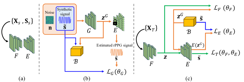
Figure 2: The proposed framework consists of one feature extractor $F$, one rPPG estimator $E$, and one latent rPPG feature generator $G$. (a) The pre-training stage: the off-the-shelf rPPG model $T=F\circ E$ is pretrained on the source training data $\{\mathbf{X}_{s},\mathbf{S}_{s}\}$. (b) The post-training stage: the sampled Gaussian noise $\mathbf{n}$ and the synthetic rPPG signal $\widetilde{\mathbf{s}}$ are used to guide the generator $G$ to generate latent rPPG features $\mathbf{z}^{G}$. (c) The inference stage of test-time adaptation: we first adapt $T$ to the incoming batch of target sample $\{\mathbf{X}_{T}\}$ to alleviate the uncertainty of the estimated rPPG signals, and then use the generated paired $\mathbf{z}^{G}$ and $\widetilde{\mathbf{s}}$ to adapt $T$ to target domain.

Compared to obtaining the source data and its statistics, fully test-time adaptation is more feasible, as fully test-time adaptation requires only the acquisition of off-the-shelf models. Therefore, the authors in [4] pioneered fully test-time adaptation by adapting the off-the-shelf models to the target domain without the need for auxiliary source statistics. Next, in [11], the authors proposed to rectify inaccurate normalization statistics to address the issue of class bias. Furthermore, the authors in [12] proposed adapting concave-convex procedure to optimize the models for fully test-time adaptation. Considering the potential of fully test-time adaptation, we firmly believe that exploring fully test-time adaptation would boost the development of the field in rPPG estimation.

II-B rPPG estimation

Remote photoplethysmography (rPPG) estimation aims to derive pulse signals from facial videos by capturing and analyzing the subtle changes in skin color for heart rate measurement. Since rPPG signals are subtle and fragile, rPPG estimation is a challenging task. rPPG estimation often performs well in the source training domain but fails to generalize effectively to the target testing domain due to new domain information and unseen heart rate ranges. In addition, due to the potential inaccuracies of the ground truth rPPG signals within source training data [1], the learned rPPG models may exhibit unstable estimations. In earlier methods [13, 14, 15], the authors focused on improving intra-domain performance but rarely addressed the cross-domain issue. These rPPG models easily overfit to the source training domain and fail to generalize to the target testing domain due to significant domain shifts. To address the cross-domain issue, many recent rPPG estimation methods have been developed to adopt domain generalization (DG) and domain adaptation (DA) techniques. For example, the authors in [2, 16] proposed adopting DG technique to address the cross-domain issue for rPPG estimation. In particular, the authors in [2] proposed to maximize the coverage of the rPPG feature space to improve the generalization capacity of rPPG extraction. In [16], the authors proposed to learn a hierarchical style-aware feature disentanglement to extracting domain-invariant and instance-specific rPPG features to enhance rPPG estimation. In addition, the authors in [3] proposed adopting domain adaptation (DA) technique to synthesize target noise to enhance the source domain training to achieve the noise reduction of rPPG estimation.

III Methodology

In this paper, we aim to tackle the test-time adaptation (TTA) problem in rPPG estimation, especially focusing on exploring potential new domain information and heart rate ranges different from the source model. To this end, we propose a novel representation learning, guided by synthetic rPPG signals, to facilitate test-time adaptation for rPPG estimation.

Given an off-the-shelf rPPG model $T$ pre-trained on the source training data $\{\mathbf{X}_{s},\mathbf{S}_{s}\}$ (where $\mathbf{X}_{s}$ indicates the source facial videos and $\mathbf{S}_{s}$ denotes the ground truth rPPG signals of $\mathbf{X}_{s}$), we propose to adapt $T$ to the incoming batch of unlabeled target facial videos $\mathbf{X}_{T}^{i}=\left\{\mathbf{x}\right\}$ and then use the adapted model to estimate the rPPG signals $\bar{\mathbf{s}}$. As shown in Figure 2 (a), the rPPG model $T=F\circ E$ is composed of one feature extractor $F$ and one rPPG estimator $E$, where $F$ is used to extract the latent rPPG feature representation and $E$ is used to estimate the rPPG signals. To overcome the challenge of estimating unseen heart rate range in $\mathbf{X}_{T}$, we specifically synthesize pseudo rPPG signals with different frequencies and then incorporate a generative module $G$ to generate latent rPPG features guided by synthetic rPPG signals. There are overall three sets of parameters, $\bm{\theta}_{F}$ of $F$, $\bm{\theta}_{E}$ of $E$ and $\bm{\theta}_{G}$ of $G$, to be optimized in the post-training stage in Figure 2 (b) for $\bm{\theta}_{G}$ and the online training (adaptation) process of the inference stage in Figure 2 (c) for $\bm{\theta}_{F}$ and $\bm{\theta}_{E}$. Below, we give the detailed description of the proposed approach.

(a)

(b)

Figure 3: Samples of (a) ground truth rPPG signal and its corresponding Power Spectral Density (PSD) and (b) synthetic rPPG signal and its corresponding PSD.

III-A Synthetic signal-guided feature learning

Given an unlabeled target facial video $\mathbf{x}\in\mathbf{X}_{T}^{i}$, we estimate its rPPG signals $\bar{\mathbf{s}}$ of $\mathbf{x}$ by,

$$\bar{\mathbf{s}}=T(\mathbf{x})=E(F(\mathbf{x}))=E(\mathbf{z})\,,$$ (1)

where $\mathbf{z}=F(\mathbf{x})$ is the latent rPPG feature. According to the heart rate range of 40 to 250 beats per minute (bpm), previous studies [17, 9] have shown that the power spectrum densities (PSDs) $\mathbf{f}$ of $\bar{\mathbf{s}}$ should fall in the frequency interval between 0.66 Hz and 4.16 Hz. Therefore, as shown in Figure 3 (a), these methods [17, 9] used the PSDs $\mathbf{f}$ to identify the frequency $f$ corresponding to the highest peak to obtain the heart rate value. However, under TTA setting, when adapting $T$ to new domains, the model may forget the previously learned HR distributions or fail to accurately estimate the range of HR which did not appear in the training sets. To tackle these challenges, we develop a synthetic signal-guided feature learning to generate the latent rPPG features covering the entire heart rate range. These generated rPPG features are used to guide the rPPG model to prevent forgetting the learned heart rate distributions and to learn the heart rates unseen in the source model.

III-A1 Synthetic rPPG signals

To resolve the forgetting problem and the issue of unseen HR distributions, we include a synthetic signal-guided generator $G$ in the post-training stage to generate latent rPPG features $\mathbf{z}^{G}$ for different heart rates. More importantly, this strategy empowers the rPPG model $T$ to effectively detect HR values unseen in the training datasets. Note that, during the post-training stage in Figure 2 (b), only an off-the-shelf rPPG model $T$ is available without any source training data.

Recall that we can use the peak frequency $f$ of PSDs $\mathbf{f}$ to derive the HR value of rPPG signals, as shown in Figure 3 (a). Therefore, after converting the human HR range (i.e., 40 to 250 bpm) in the corresponding frequency value $f$ of $[0.66,4.16]$ Hz, we propose to synthesize a set of pseudo rPPG signals $\widetilde{\mathbf{s}}$, denoted as $\widetilde{\mathcal{S}}=\{\widetilde{\mathbf{s}}\}$, according to these frequencies $f$ in the post-training stage. To synthesize $\widetilde{\mathbf{s}}$, we adopt the simplified formulation proposed in [18] by

$$\begin{split}\widetilde{\mathbf{s}}&=M\sin(2\pi ft+\phi)+0.1\cdot M\sin(2\pi(2f)t+\phi),\end{split}$$ (2)

where $\operatorname{sin}(\cdot)$ is a sine function, $M$ denotes the magnitude randomly sampled from $[0,1]$, $f$ is the frequency transformed from HR value, $t$ denotes time, and $\phi$ is the phase offset randomly sampled from $[0,2\pi]$. Figure 3 (b) shows examples of using specific transformed frequency (i.e., 90 bpm to 1.5 Hz) to synthesize the pseudo rPPG signals. We see that synthetic and ground truth rPPG signals have highly similar frequencies and PSDs.

III-A2 Generative feature learning

We now describe how we include a conditional generator $G$ in the proposed synthetic signal-guided generative feature learning. As illustrated in Figure 2 (b), we propose the feature generation process by using $G$ conditioned on a given synthetic rPPG signal $\widetilde{\mathbf{s}}$ as well as the noise $\mathbf{n}$ sampled from a unit Gaussian prior, $\mathbf{n}\sim\mathcal{N}(0,I)$, to generate the latent rPPG features $\mathbf{z}^{G}$ by.

$$\mathbf{z}^{G}\,\leftarrow G(\mathbf{n}|\widetilde{\mathbf{s}};\bm{\theta}_{G}).$$ (3)

With Equation (3), the synthetic signal-guided generative process incorporates another aspect of input, denoted as $\mathbf{z}^{G}$, to enhance the TTA of the rPPG model $T$. As shown in Figure 2 (b), the synthetic signal-guided feature learning pipeline involves the generator $G$ and the estimator $E$, thereby incorporating the parameters $\bm{\theta}_{G}$ and $\bm{\theta}_{E}$. We adopt an optimization strategy to learn $\bm{\theta}_{G}$ by fixing $\bm{\theta}_{E}$. In particular, we consider minimizing the following loss:

$$\begin{split}\mathcal{L}_{G}(\bm{\theta}_{G})&=\sum\nolimits_{\widetilde{\mathbf{s}}\in\widetilde{\mathcal{S}}}1-\rho(E(G(\mathbf{n}|\widetilde{\mathbf{s}};\bm{\theta}_{G})),\widetilde{\mathbf{s}})\\ &=\sum\nolimits_{\widetilde{\mathbf{s}}\in\widetilde{\mathcal{S}}}1-\rho(E(\mathbf{z}^{G}),\widetilde{\mathbf{s}}),\end{split}$$ (4)

where $\rho(\bar{\mathbf{s}},\widetilde{\mathbf{s}})=\frac{Cov(\bar{\mathbf{s}},\widetilde{\mathbf{s}})}{\sqrt{Cov(\bar{\mathbf{s}},\widetilde{\mathbf{s}})}\sqrt{Cov(\bar{\mathbf{s}},\widetilde{\mathbf{s}})}}$ is the Pearson correlation between $\bar{\mathbf{s}}=E(\mathbf{z}^{G})$ and $\widetilde{\mathbf{s}}$, and $Cov(\bar{\mathbf{s}},\widetilde{\mathbf{s}})$ denotes the covariance between $\bar{\mathbf{s}}$ and $\widetilde{\mathbf{s}}$. To learn $\bm{\theta}_{G}$, we define the optimization problem as follows:

$$\bm{\theta}_{G}^{*}=\mathop{\mathrm{arg}\,\mathrm{min}}_{\bm{\theta}_{G}}\mathcal{L}_{G}(\bm{\theta}_{G}).$$ (5)

Figure 4: Illustration of the hierarchical memory bank $\mathcal{B}$.

III-A3 Frequency-aware memory buffer

So far we have established a synthetic signal-guided feature learning formulation to generate the paired pseudo rPPG signals and latent features, i.e., $\{(\widetilde{\mathbf{s}},\mathbf{z}^{G})\}$. Next, we design a hierarchical memory bank $\mathcal{B}$ to store the generated pairs$(\widetilde{\mathbf{s}},\mathbf{z}^{G})$ to facilitate the rPPG estimation during test-time adaptation stage. As shown in Figure LABEL:fig:MB, in $\mathcal{B}$, we keep $I$ sub-memory banks to store the all frequency values corresponding to HRs within the HR range. For each frequency $f$, we maintain a fixed-size sub-memory buffer that includes $J$ generated pairs $(\widetilde{\mathbf{s}},\mathbf{z}^{G})$. When the sub-memory buffer of $\mathcal{B}$ is fully stored, we adopt the First In First Out (FIFO) scheme to update the sub-memory buffer.

(a)

(b)

Figure 5: Samples of the entropy $H(\mathbf{f})$ from (a) the estimated rPPG signal $\bar{\mathbf{s}}$ and (b) the ground truth rPPG signal $\mathbf{s}$.

III-B Feature-enhanced test-time rPPG estimation

Having described the synthetic signal-guided generative feature learning, we now need to elucidate how the remaining parameters (i.e., $\bm{\theta}_{F}$ and $\bm{\theta}_{E}$) are optimized during the online training (adaptation) process of the inference stage within TTA, as shown in Figure 2 (c).

III-B1 Spectral-based entropy minimization

Since the unlabeled target facial video $\mathbf{x}\in\mathbf{X}_{T}^{i}$ may contain new domain information, the rPPG model $T$ may produce the estimated rPPG signals $\bar{\mathbf{s}}$ with higher uncertainty. In Figure 5, by following the approach described in [19] to estimate the entropy $H(\mathbf{f})$ of PSDs derived from (a) the estimated rPPG signal $\bar{\mathbf{s}}$ and (b) the ground truth rPPG signal $\mathbf{s}$ for the same target video, we observe that $\bar{\mathbf{s}}$ indeed exhibits higher entropy compared to $\mathbf{s}$, despite their corresponding HR values being highly similar. To alleviate the uncertainty within $\bar{\mathbf{s}}$, we propose a novel spectral-based entropy loss to adapt the model $T$ to new domains by,

$$\mathcal{L}_{T}(\bm{\theta}_{F},\bm{\theta}_{E})=H(\mathbf{f})=-\sum^{b}_{i=a}\mathbf{f}_{i}\log(\mathbf{f}_{i}),$$ (6)

where $\mathbf{f}$ is the PSD of $\bar{\textbf{s}}$, $\mathbf{f}_{i}$ denotes the $i$-th frequency bin within $\mathbf{f}$, and $a$ and $b$ represent the lower and upper bounds of the frequency (i.e., 0.66 Hz and 4.16 Hz).

III-B2 Feature-enhanced rPPG estimation

Now, with the generated pairs $(\widetilde{\mathbf{s}},\mathbf{z}^{G})$ by $G$ from $\mathcal{B}$, the concerns regarding forgotten and unseen HR distributions are no longer issues. More specifically, we propose to use the generated pairs within $\mathcal{B}$ to enhance the estimator $E$ fine-tuning. We thus have

$$\begin{split}\mathcal{L}_{E}(\bm{\theta}_{E})=\sum\nolimits_{\widetilde{\mathbf{s}},\mathbf{z}^{G}\in\mathcal{B}}1-\rho(E(\mathbf{z}^{G};\bm{\theta}_{E}),\widetilde{\mathbf{s}}).\end{split}$$ (7)

Subsequently, our next goal is to fine-tune the extractor $F$ to align the extracted rPPG features $\textbf{z}=F(\mathbf{x})$ and the generated rPPG features $\textbf{z}^{G}$ from the similar HRs. Unlike previous rPPG estimation methods [17, 9], which proposed to dichotomize the rPPG features as either positive pairs or negative pairs based on different HR values to learn the rPPG features, the authors in [20] found that the periodic features exhibit a continuous similarity change in periodic feature measurement when the feature frequency varies. Inspired by [20], we propose an effective adaptive feature alignment to align the latent rPPG features z and $\textbf{z}^{G}$ from similar HRs. Thus, to effectively align the latent rPPG features in adapting the extractor $F$, we introduce an additional regularization loss, namely,

$$\begin{split}\mathcal{L}_{F}(\bm{\theta}_{F})=\sum\nolimits_{\mathbf{z}^{G}\in\mathcal{B}}\lvert e^{\frac{-1}{2}(\frac{f_{\mathbf{z}}-f_{\mathbf{z}^{G}}}{\sigma})^{2}}-\cos(F(\mathbf{x};\bm{\theta}_{F}),\mathbf{z}^{G})\rvert,\end{split}$$ (8)

where $f_{\mathbf{z}},f_{\mathbf{z}^{G}}\in[0.66,4.16]$ Hz are the frequencies corresponding to the HR values of the estimated rPPG signals $E(\mathbf{z})$ and $E(\mathbf{z}^{G})$, $\cos(\cdot)$ is the cosine function, and $\sigma$ is a predefined constant set to 0.04 based on empirical findings. As shown in Figure 6, we observe that different values of $\sigma$ enable guiding the proposed adaptive feature alignment to align similar rPPG features from different HR ranges.

Figure 6: Illustration of adaptive weights from $e^{\frac{-1}{2}(\frac{f_{\mathbf{z}}-f_{\mathbf{z}^{G}}}{\sigma})^{2}}$ for aligning rPPG features from different HR ranges.

Finally, analogous to (5), by freezing the parameters $\bm{\theta}_{G}$ of the generator $G$, the model fine-tuning of $T=F\circ E$, can be achieved with

$$\bm{\theta}_{F}^{*},\bm{\theta}_{E}^{*}=\mathop{\mathrm{arg}\,\mathrm{min}}_{\bm{\theta}_{F},\bm{\theta}_{E}}\mathcal{L}_{E}(\bm{\theta}_{E})+\alpha\mathcal{L}_{F}(\bm{\theta}_{F})+\beta\mathcal{L}_{T}(\bm{\theta}_{F},\bm{\theta}_{E}),$$ (9)

where $\alpha$ and $\beta$ are the weight factors. In all our experiments, we empirically set $\alpha=0.5$ and $\beta=0.1$.

IV Experiment

(a)	(b)

(c)	(d)

Figure 7: Illustration of HR distributions on different rPPG datasets, including (a) COHFACE [21], (b) PURE [22], (c) UBFC-rPPG [23], and (d) VIPL-HR [13].

TABLE I: Different testing protocols from the proposed TTA-rPPG benchmark.

Protocols	Pre-training sets	Testing sets
V $\rightarrow$ C	45-180 bpm	45-100 bpm
V $\rightarrow$ P		40-165 bpm
V $\rightarrow$ U		55-140 bpm
V $\rightarrow$ [C,P,U]		40-165 bpm
C $\rightarrow$ P	45-100 bpm	40-165 bpm
C $\rightarrow$ U		55-140 bpm
C $\rightarrow$ V		45-180 bpm
C $\rightarrow$ [P,U,V]		40-180 bpm

IV-A Datasets

IV-A1 PURE

The dataset PURE [22] comprises 60 RGB videos featuring 10 subjects. Each subject is recorded under six distinct conditions, including sitting still, talking, slow and fast head translation, and small and large head rotation, with each video lasting approximately one minute. All videos are captured at a resolution of 640 × 480 pixels and a frame rate of 30 fps.

IV-A2 COHFACE

The dataset COHFACE [21] comprises 160 RGB videos featuring 40 subjects under studio and natural light. All videos are captured at a resolution of 640 × 480 pixels and a frame rate of 20 fps.

IV-A3 UBFC-rPPG

The dataset UBFC-rPPG [23] comprises 42 RGB videos under sunlight and indoor illumination conditions. Because participants will play a time-sensitive mathematical game in the videos, the heart rate range will be larger. All videos are captured at a resolution of 640 × 480 pixels and a frame rate of 30 fps.

IV-A4 VIPL-HR

The dataset VIPL-HR [13] comprises 2,378 RGB videos of 107 subjects under head movements, illumination variations, and acquisition device changes.

IV-B Fully Test-Time Adaptation Benchmark for rPPG Estimation (TTA-rPPG)

In this paper, we propose new fully Test-Time Adaptation benchmark for rPPG estimation (TTA-rPPG) to study the challenges posed by new domain information and unseen heart rate distributions. We construct the TTA-rPPG benchmark based on four publicly available rPPG datasets, including COHFACE [21] (denoted as C), PURE [22] (denoted as P), UBFC-rPPG [23] (denoted as U), and VIPL-HR [13] (denoted as V). As shown in Figure 7, we analyze the HR distributions of different rPPG datasets by examining the quantity of heart rates from sampled 10-second clips. We observe that the HR range of C is constrained to distribute between 40 to 100 bpm. By contrast, the HR range of datasets U, P, and V is widely distributed between 40 and 180 bpm. Therefore, in Table I, we design the different testing protocols for TTA-rPPG benchmark to evaluate the efficacy of rPPG models when encountering target data containing either (1) new domain information and seen HR distributions or (2) new domain information and unseen HR distributions under test-time adaptation scenario. In addition, we also design the protocols, i.e., V$\rightarrow$ [C,P,U] and C$\rightarrow$ [P,U,V] by mixing videos from different datasets to simulate a real-world scenario where data is non-independent and identically distributed (non-i.i.d) [24]. To obtain the pre-trained models for each protocol, we adopt a similar approach to previous classification-based TTA methods [4, 25, 26], which only use the vanilla cross-entropy loss to pre-train classification models. Therefore, we propose adopting the network architecture (Physnet) proposed in [27] as $T$ and using the simple negative Pearson correlation loss [14, 28] to pre-train the rPPG models for each protocol.

IV-C Evaluation Metrics and Implementation Details

We evaluate our method on the proposed TTA-rPPG benchmark and report the results using different evaluation metrics, including Mean Absolute Error (MAE) and Root Mean Square Error (RMSE) across all target datasets. During inference stage, we refer to [17, 9] to decompose each test video into non-overlapping 10s clips and then estimate the rPPG signals of each clip to calculate PSD for deriving HR of each clip.

TABLE II: Ablation study on the protocols V$\rightarrow$ [C,P,U] and C$\rightarrow$ [P,U,V], using different loss combinations.

Loss Terms			V$\rightarrow$ [C,P,U]		C$\rightarrow$ [P,U,V]
$\mathcal{L}_{T}$	$\mathcal{L}_{E}$	$\mathcal{L}_{F}$	MAE$\downarrow$	RMSE$\downarrow$	MAE$\downarrow$	RMSE$\downarrow$
-	-	-	21.41	24.16	28.72	30.44
✓	-	-	17.27	22.29	21.03	23.54
✓	✓	-	14.53	16.94	15.23	17.95
✓	✓	✓	11.14	12.08	12.75	14.48

Figure 8: Illustration of (a) facial images and (b)-(e) saliency maps [29] generated by different $T$. For a good rPPG estimator, the visualized saliency maps should have a large response on facial skin regions.

IV-D Ablation Study

IV-D1 Comparison between Different Loss Terms

In Table II, we compare using different combinations of loss terms to update $T=F\circ E$ during the online training (adaptation) process of inference stage. Here, we test various rPPG models on the proposed protocols V$\rightarrow$ [C,P,U] and C$\rightarrow$ [P,U,V] from Table I. In addition, we use two examples to visualize the saliency maps to demonstrate the efficacy of different combinations of loss terms, as shown in Figure 8.

First, we use the fixed pre-trained models without any online training (adaptation) process as the baseline. We observe that the performances of the baseline models are limited, and the saliency maps in Figure 8 (b) appear blurred due to the presence of new domain information and unseen HR distributions in the target data.

Next, we include $\mathcal{L}_{T}$ to fine-tune $F$ and $E$. We see that the proposed spectral-based entropy minimization effectively adapts the model $T$ to learn the target domain information. The saliency maps in Figure 8 (c) also show improvement compared to Figure 8 (b).

Moreover, we include $\mathcal{L}_{E}$ and use the paired $(\widetilde{\mathbf{s}},\mathbf{z}^{G})$ stored from $\mathcal{B}$ to enhance the adaptation of $E$. Because the generator $G$ guided by the synthetic rPPG signals $\widetilde{\mathbf{s}}$ is able to generate latent rPPG features capable of producing the estimated rPPG signals similar to $\widetilde{\mathbf{s}}$, we see that the generated $(\widetilde{\mathbf{s}},\mathbf{z}^{G})$ indeed facilitates the adaptation of $E$ to effectively estimate the rPPG signals and measure the HRs unseen within the source data. In addition, we see the saliency maps in Figure 8 (d) more accurately concentrate on facial regions compared to Figure 8 (c).

Finally, when including $\mathcal{L}_{F}$, we achieve the best performance and saliency maps in Figure 8 (e) by continually aligning the extracted rPPG features $\mathbf{z}^{G}$ to the generated rPPG features $\mathbf{z}^{G}$. The overall improvement verifies the superiority of the proposed synthetic signal-guided feature learning.

TABLE III: Ablation study on the protocols V$\rightarrow$ [C,P,U] and C$\rightarrow$ [P,U,V], using different optimization strategies.

Updating parameters	V$\rightarrow$ [C,P,U]		C$\rightarrow$ [P,U,V]		FPS
	MAE$\downarrow$	RMSE$\downarrow$	MAE$\downarrow$	RMSE$\downarrow$
BatchNorm layers	15.85	19.75	20.14	21.71	1146.15
Entire model $T$	11.14	12.08	12.75	14.48	912.12

IV-D2 Comparison between Different Optimization Strategies

In Table III, we compare using different optimization strategies to fine-tune $T$ under the same loss $\mathcal{L}_{T}+\mathcal{L}_{E}+\mathcal{L}_{F}$ during the online training (adaptation) process. We first refer to previous classification-based TTA methods [4, 7] that only update the batch normalization (BN) layers. We see that updating BN layers enables rapid response and aids $T$ in learning target domain information. However, updating only BN layers is insufficient to effectively adapt $T$ to learn unseen HR distributions, resulting in unsatisfactory performance. By contrast, when updating the entire model $T$, the significant improvement demonstrates that $T$ better adapts to the target data containing new domain information and unseen HR distributions without encountering significant speed degradation.

TABLE IV: Ablation study on the protocols V$\rightarrow$ [C,P,U] and C$\rightarrow$ [P,U,V], using different feature alignments (FA).

Methods	V$\rightarrow$ [C,P,U]		C$\rightarrow$ [P,U,V]
	MAE$\downarrow$	RMSE$\downarrow$	MAE$\downarrow$	RMSE$\downarrow$
Dichotomous FA [17, 9]	13.85	15.88	14.71	16.25
Adaptive FA	11.14	12.08	12.75	14.48

TABLE V: Ablation study on the protocols V$\rightarrow$ [C,P,U] and C$\rightarrow$ [P,U,V], using different memory banks (MB).

Methods	V$\rightarrow$ [C,P,U]		C$\rightarrow$ [P,U,V]
	MAE$\downarrow$	RMSE$\downarrow$	MAE$\downarrow$	RMSE$\downarrow$
Vanilla MB	13.18	14.42	14.78	15.50
Hierarchical MB	11.14	12.08	12.75	14.48

TABLE VI: Ablation study on different network architectures.

Network $T$	Method	C$\rightarrow$ [P,U,V]
		MAE$\downarrow$	RMSE$\downarrow$	Model size	GFLOPs	FPS
PhysNet [27]	No adaptation	28.72	30.44	2.93MB	196.72	4327.01
	Ours	12.75	14.48			912.12
PhysFormer [30]	No adaptation	24.16	28.67	28.15MB	296.06	1597.051
	Ours	11.48	12.71			464.87

TABLE VII: HRV and HR estimation results on UBFC-rPPG.

Method	LF (n.u.)			HF (n.u.)			LF/HF			RF(Hz)			HR(bpm)
	STD$\downarrow$	RMSE$\downarrow$	R$\uparrow$	STD$\downarrow$	RMSE$\downarrow$	R$\uparrow$	STD$\downarrow$	RMSE$\downarrow$	R$\uparrow$	STD$\downarrow$	RMSE$\downarrow$	R$\uparrow$	MAE$\downarrow$	RMSE$\downarrow$
RErPPGNet [1]	0.128	0.194	0.667	0.128	0.194	0.667	0.452	0.603	0.496	0.050	0.060	0.011	2.00	2.40
NEST [2]	0.131	0.216	0.259	0.131	0.216	0.259	0.539	0.800	0.236	0.048	0.060	0.158	1.29	4.97
Dual-bridging [3]	0.138	0.172	0.397	0.138	0.172	0.397	0.500	0.556	0.227	0.069	0.087	0.187	0.16	0.57
No adaptation	0.161	0.227	0.291	0.161	0.227	0.291	0.592	0.862	0.242	0.116	0.152	0.174	2.84	3.68
Ours	0.055	0.103	0.771	0.055	0.103	0.771	0.167	0.219	0.790	0.062	0.123	0.270	0.40	0.69

TABLE VIII: Experimental comparisons on the proposed TTA-rPPG benchmark.

Type	Method	V $\rightarrow$ P		V $\rightarrow$ U		V $\rightarrow$ C		V $\rightarrow$ [C,P,U]
		MAE$\downarrow$	RMSE$\downarrow$	MAE$\downarrow$	RMSE$\downarrow$	MAE$\downarrow$	RMSE$\downarrow$	MAE$\downarrow$	RMSE$\downarrow$
DG	RErPPG-Net [1] (ECCV 22)	13.26	14.88	13.11	18.68	13.48	15.41	18.64	21.31
	NEST [2] (CVPR 23)	13.21	19.49	7.68	10.56	12.53	14.60	16.08	20.38
DA	Dual-bridging [3] (CVPR 23)	6.58	9.16	5.14	8.44	10.25	11.98	10.25	12.81
TTA	No adaptation	15.26	18.89	14.64	18.50	17.19	20.01	21.41	24.16
	Ours	3.33	4.87	5.60	7.16	8.31	9.16	11.14	12.08
Type	Method	C $\rightarrow$ P		C $\rightarrow$ U		C $\rightarrow$ V		C $\rightarrow$ [P,U,V]
		MAE$\downarrow$	RMSE$\downarrow$	MAE$\downarrow$	RMSE$\downarrow$	MAE$\downarrow$	RMSE$\downarrow$	MAE$\downarrow$	RMSE$\downarrow$
DG	RErPPG-Net [1] (ECCV 22)	13.53	14.16	16.13	17.08	30.52	34.10	26.51	29.86
	NEST [2] (CVPR 23)	16.25	23.88	17.99	22.84	24.90	28.93	25.30	29.85
DA	Dual-bridging [3] (CVPR 23)	0.94	1.51	6.00	7.67	23.99	25.86	25.19	26.59
TTA	No adaptation	17.93	20.12	19.32	21.35	31.51	34.06	28.72	30.44
	Ours	1.45	2.24	3.60	5.26	12.36	13.08	12.75	14.48

IV-D3 Comparison between Different Feature Alignments

In Table IV, we compare using different feature alignments (FA) to align the extracted rPPG features $\textbf{z}=F(\mathbf{x})$ and the generated rPPG features $\textbf{z}^{G}$. First, we adopt the dichotomous feature alignment [17, 9] to align $\mathbf{z}=F(\mathbf{x})$ and $\mathbf{z}^{G}$ from the same HR and to push $\mathbf{z}=F(\mathbf{x})$ and $\mathbf{z}^{G}$ from different HRs. Next, by adopting the proposed adaptive feature alignment to align $\mathbf{z}=F(\mathbf{x})$ and $\mathbf{z}^{G}$ from the similar HRs, the adaptation of $T$ is improved. This performance enhancement also coincides with the finding observed in [20] that learning similar features of periodic signals with similar frequencies (i.e., HRs) indeed facilitates rPPG estimation.

Figure 9: Ablation study on the protocol V$\rightarrow$ [C,P,U], using different sub-memory bank sizes.

IV-D4 Comparison between Different Memory Banks

In Table V, we compare using different memory banks (MB) of the same total size to store the generated $(\widetilde{\mathbf{s}},\mathbf{z}^{G})$ under the same First In First Out (FIFO) scheme. Because the vanilla MB adopts the FIFO scheme during the training of $G$, it cannot guarantee that the stored pairs $(\widetilde{\mathbf{s}},\mathbf{z}^{G})$ cover the entire HR range. By contrast, the proposed hierarchical MB ensures that the stored pairs $(\widetilde{\mathbf{s}},\mathbf{z}^{G})$ cover the entire HR range to effectively enhance the adaptation of $T$.

IV-D5 Comparison between Different Sizes of Memory Bank

In Figure 9, we compare using different sub-memory bank sizes $N_{\mathcal{B}}$ ($N_{\mathcal{B}}$ = 1, 2, 4, 6, 8 and 16) in $\mathcal{B}$ on the protocol V$\rightarrow$ [C,P,U] and show the results in terms of MAE and RMSE. First, We observe that the performance steadily improves as $N_{\mathcal{B}}$ increases from 1 to 6 and reaches the best performance at $N_{\mathcal{B}}=6$. These results demonstrate that larger sub-memory banks indeed facilitate better adaptation of the rPPG models to unseen HR distributions. Next, we see that the performance does not improve as $N_{\mathcal{B}}$ increases from 8 to 16. This performance plateau might indicate that the memory bank has reached a state of overcompleteness. Therefore, based on this ablation study, we empirically set $N_{\mathcal{B}}=6$ for subsequent experiments.

Figure 10: Ablation study on the protocol V$\rightarrow$ [C,P,U], using different $\sigma$ in Equation (8).

IV-D6 Comparison between Different $\sigma$

In Figure 10, we compare using different $\sigma$ in Equation (8) to align similar rPPG features from different HR ranges. Note that, different values of $\sigma$ corresponding to valid HR ranges are given in Figure 6. Because rPPG features corresponding to similar HRs exhibit proximity in the latent feature space [20], we see that aligning rPPG features within HR range of minor difference (i.e., $\sigma\leq 0.04$, corresponding to HR difference of less than 5) does indeed facilitate the feature alignment process, as shown in Figure 10. In addition, when aligning rPPG features within HR range of larger difference, their corresponding rPPG features exhibit differences that hinder effective feature alignment.

IV-D7 Comparison between Different Network Architectures

In Table VI, we investigate the impact of different network architectures using the same loss $\mathcal{L}_{T}+\mathcal{L}_{E}+\mathcal{L}_{F}$ on the most challenging protocol C $\rightarrow$ [P,U,V]. The results in Table VI verify robust transferability of the proposed method using different network architectures. Moreover, the results in Table VI show that, larger and more powerful network architectures indeed yield better performance but have lower inference speed due to the increased number of parameters.

IV-D8 HRV Analysis

We conduct HRV and HR estimation on UBFC-rPPG and show the result in Table VII. The results in Table VII and Table 6 all demonstrate the effectiveness of the proposed method in both intra-domain and cross-domain testing. In addition, our method also produces better quality rPPG waveforms to improve the heart rate measurement.

IV-E Experimental Comparisons on the proposed TTA-rPPG benchmark

In Table VIII, we present the evaluation results of the proposed method and compare with other domain generalization (DG) and domain adaptation (DA) methods on TTA-rPPG benchmark. We re-implement all the compared methods and fix the pre-trained rPPG models $T$ during the inference stage, denoted as ”No adaptation”. First, we observe that ”No adaptation” yields poorer performance than the DG methods [1, 2] because ”No adaptation”, trained solely by negative Pearson correlation loss, fails to generalize well to the target domain. Next, we observe that the DA method [3], which utilizes labeled source data and unlabeled target data, effectively adapts the rPPG models to the target domain to achieve better performances. Although these DG and DA methods may perform well within the seen HR distribution seen in the source data, they may overfit to that distribution and exhibit degraded performance when facing unseen HR distributions. With the generated rPPG signals and features, our method effectively adapt $T$ to learn estimating the HRs unseen in the source training data. By comparing the results of experimenting with C$\rightarrow$ [U], C$\rightarrow$ [V], and C$\rightarrow$ [P,U,V], it can be seen that the proposed method benefits from using the generated rPPG signals and features.

V Conclusion

In this paper, we introduce a new benchmark TTA-rPPG and propose a novel synthetic signal-guided generative feature learning approach to address challenges of TTA in rPPG estimation. We first design an effective spectral-based entropy minimization mechanism to adapt the model to new domain. Next, we propose a novel synthetic signal-guided generative feature learning to resolve the issue of unseen HR distributions. In addition, we propose an adaptive feature alignment to reliably estimate the unlabeled target data. Our experimental results on the proposed benchmark TTA-rPPG demonstrate the superior performance of the proposed method on handling realistic TTA scenarios.

References

- [1] C. Hsieh, W. Chung, and C. Hsu, “Augmentation of rppg benchmark datasets: Learning to remove and embed rppg signals via double cycle consistent learning from unpaired facial videos,” in European Conf. Comput. Vis. Springer, 2022, pp. 372–387.
- [2] H. Lu, Z. Yu, X. Niu, and Y.-C. Chen, “Neuron structure modeling for generalizable remote physiological measurement,” in Proceedings of the IEEE/CVF Conference on Computer Vision and Pattern Recognition, 2023, pp. 18 589–18 599.
- [3] J. Du, S. Liu, B. Zhang, and P. Yuen, “Dual-bridging with adversarial noise generation for domain adaptive rppg estimation,” in Proc. IEEE/CVF Conf. Comput. Vis. Pattern Recog., 2023, pp. 10 355–10 364.
- [4] D. Wang, E. Shelhamer, S. Liu, B. Olshausen, and T. Darrell, “Tent: Fully test-time adaptation by entropy minimization,” in International Conference on Learning Representations, 2021.
- [5] W. Lin, M. J. Mirza, M. Kozinski, H. Possegger, H. Kuehne, and H. Bischof, “Video test-time adaptation for action recognition,” in Proceedings of the IEEE/CVF Conference on Computer Vision and Pattern Recognition, 2023, pp. 22 952–22 961.
- [6] H. Lim, B. Kim, J. Choo, and S. Choi, “Ttn: A domain-shift aware batch normalization in test-time adaptation,” in The Eleventh International Conference on Learning Representations, 2022.
- [7] S. Park, S. Yang, J. Choo, and S. Yun, “Label shift adapter for test-time adaptation under covariate and label shifts,” in Proceedings of the IEEE/CVF International Conference on Computer Vision, 2023, pp. 16 421–16 431.
- [8] S. Choi, S. Yang, S. Choi, and S. Yun, “Improving test-time adaptation via shift-agnostic weight regularization and nearest source prototypes,” in European Conference on Computer Vision, 2022, pp. 440–458.
- [9] Z. Sun and X. Li, “Contrast-phys: Unsupervised video-based remote physiological measurement via spatiotemporal contrast,” in Proc. European Conf. Comput. Vis., 2022, pp. 492–510.
- [10] J. Zhang, L. Qi, Y. Shi, and Y. Gao, “Domainadaptor: A novel approach to test-time adaptation,” in Proceedings of the IEEE/CVF International Conference on Computer Vision, 2023, pp. 18 971–18 981.
- [11] B. Zhao, C. Chen, and S.-T. Xia, “Delta: degradation-free fully test-time adaptation,” arXiv preprint arXiv:2301.13018, 2023.
- [12] M. Boudiaf, R. Mueller, I. Ben Ayed, and L. Bertinetto, “Parameter-free online test-time adaptation,” in Proceedings of the IEEE/CVF Conference on Computer Vision and Pattern Recognition, 2022, pp. 8344–8353.
- [13] X. Niu, S. Shan, H. Han, and X. Chen, “Rhythmnet: End-to-end heart rate estimation from face via spatial-temporal representation,” IEEE Trans. Image Process., vol. 29, pp. 2409–2423, 2020.
- [14] Y. Tsou, Y. Lee, and C. Hsu, “Multi-task learning for simultaneous video generation and remote photoplethysmography estimation,” in Proc. Asian Conf. Comput. Vis., 2020, pp. 392–407.
- [15] E. Lee, E. Chen, and C.-Y. Lee, “Meta-rppg: Remote heart rate estimation using a transductive meta-learner,” in Computer Vision–ECCV 2020: 16th European Conference, Glasgow, UK, August 23–28, 2020, Proceedings, Part XXVII 16. Springer, 2020, pp. 392–409.
- [16] J. Wang, H. Lu, A. Wang, Y. Chen, and D. He, “Hierarchical style-aware domain generalization for remote physiological measurement,” IEEE Journal of Biomedical and Health Informatics, 2023.
- [17] J. Gideon and S. Stent, “The way to my heart is through contrastive learning: Remote photoplethysmography from unlabelled video,” in Proc. IEEE/CVF Int. Conf. Comput. Vis., 2021, pp. 3995–4004.
- [18] X. Niu, H. Han, S. Shan, and X. Chen, “Synrhythm: Learning a deep heart rate estimator from general to specific,” in 2018 24th international conference on pattern recognition (ICPR). IEEE, 2018, pp. 3580–3585.
- [19] J.-F. Bercher and C. Vignat, “Estimating the entropy of a signal with applications,” IEEE transactions on signal processing, vol. 48, no. 6, pp. 1687–1694, 2000.
- [20] Y. Yang, X. Liu, J. Wu, S. Borac, D. Katabi, M.-Z. Poh, and D. McDuff, “Simper: Simple self-supervised learning of periodic targets,” in The Eleventh International Conference on Learning Representations, 2023. [Online]. Available: https://openreview.net/forum?id=EKpMeEV0hOo
- [21] G. Heusch, A. Anjos, and S. Marcel, “A reproducible study on remote heart rate measurement,” arXiv preprint arXiv:1709.00962, 2017.
- [22] R. Stricker, S. Müller, and H. Gross, “Non-contact video-based pulse rate measurement on a mobile service robot,” in Proc. 23rd IEEE Int. Symp. Robot Human Interactive Commun., 2014, pp. 1056–1062.
- [23] S. Bobbia, R. Macwan, Y. Benezeth, A. Mansouri, and J. Dubois, “Unsupervised skin tissue segmentation for remote photoplethysmography,” Pattern Recog. Lett., vol. 124, pp. 82–90, 2019.
- [24] T. Gong, J. Jeong, T. Kim, Y. Kim, J. Shin, and S. Lee, “Note: Robust continual test-time adaptation against temporal correlation,” Adv. in Neural Inf. Proc. Sys., vol. 35, pp. 27 253–27 266, 2022.
- [25] M. Jang, S. Chung, and H. W. Chung, “Test-time adaptation via self-training with nearest neighbor information,” in The 11th Int. Conf. on Learn. Representations, 2023. [Online]. Available: https://openreview.net/forum?id=EzLtB4M1SbM
- [26] S. Niu, J. Wu, Y. Zhang, Z. Wen, Y. Chen, P. Zhao, and M. Tan, “Towards stable test-time adaptation in dynamic wild world,” in Int. Conf. Learn. Representations, 2023.
- [27] Z. Yu et al., “Remote photoplethysmograph signal measurement from facial videos using spatio-temporal networks,” in BMVC, 2019.
- [28] Y. Tsou, Y. Lee, C. Hsu, and S. Chang, “Siamese-rppg network: Remote photoplethysmography signal estimation from face videos,” in Proc. 35th Annu. ACM Symp. Appl. Comput., 2020, pp. 2066–2073.
- [29] K. Simonyan, A. Vedaldi, and A. Zisserman, “Deep inside convolutional networks: Visualising image classification models and saliency maps,” Proc. 2nd Int. Conf. Learn. Representations, 2014.
- [30] Z. Yu, Y. Shen, J. Shi, H. Zhao, P. Torr, and G. Zhao, “Physformer: facial video-based physiological measurement with temporal difference transformer,” in Proc. IEEE/CVF Conf. Comput. Vis. Pattern Recog., 2022, pp. 4186–4196.