Combining Climate Models using Bayesian Regression Trees and Random Paths

Abstract

Climate models, also known as general circulation models (GCMs), are essential tools for climate studies. Each climate model may have varying accuracy across the input domain, but no single model is uniformly better than the others. One strategy to improving climate model prediction performance is to integrate multiple model outputs using input-dependent weights. Along with this concept, weight functions modeled using Bayesian Additive Regression Trees (BART) were recently shown to be useful for integrating multiple Effective Field Theories in nuclear physics applications. However, a restriction of this approach is that the weights could only be modeled as piecewise constant functions. To smoothly integrate multiple climate models, we propose a new tree-based model, Random Path BART (RPBART), that incorporates random path assignments into the BART model to produce smooth weight functions and smooth predictions of the physical system, all in a matrix-free formulation. The smoothness feature of RPBART requires a more complex prior specification, for which we introduce a semivariogram to guide its hyperparameter selection. This approach is easy to interpret, computationally cheap, and avoids an expensive cross-validation study. Finally, we propose a posterior projection technique to enable detailed analysis of the fitted posterior weight functions. This allows us to identify a sparse set of climate models that can largely recover the underlying system within a given spatial region as well as quantifying model discrepancy within the model set under consideration. Our method is demonstrated on an ensemble of 8 GCMs modeling the average monthly surface temperature.

1 Introduction

Complex natural phenomena are often modeled using computer simulators – models that incorporate theoretical knowledge to approximate an underlying system. In climate applications, these simulators, or General Circulation Models (GCMs), have been widely used to understand a variety of climate features such as temperature or precipitation (Eyring et al., 2016). Many GCMs have been developed over time and each one tends to have varying fidelity across different subregions of the world. This implies that no universally best model exists. For example, Figure 1 displays the difference between the simulated average monthly surface temperature in the northeastern hemisphere for April 2014 from three different climate models and the observed data. This figure demonstrates that the residuals (and thus the fidelity) of each GCM differs across the various spatial regions. In particular, greater variation in residuals are observed over land. Specific residual patterns tend to mimic the changes in elevation, which suggests each GCM accounts for elevation in different manners.

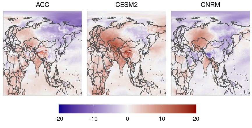
Figure 1: The difference in temperature (degrees Celsius) between the output from three different simulators and the observed average monthly surface temperature for April 2014.

Multi-model ensembles are often used to help improve global prediction of the system (Tebaldi and Knutti, 2007; Sansom et al., 2021). Various approaches exist for combining the outputs from multiple GCMs. A common approach is to explicitly combine the outputs from $K$ different GCMs using a linear combination or weighted average, usually in a pointwise manner for a specific latitude and longitude. For example, Knutti et al. (2017) and Tebaldi and Knutti (2007) define performance-based weights. Giorgi and Mearns (2002) define Reliability Ensemble Averaging (REA), which weight the GCMs based on model performance and model convergence. More traditional regression-based models assume the underlying process can be modeled as a linear combination of the individual GCMs (Tebaldi and Knutti, 2007). Vrac et al. (2024) propose a density-based approach that combines the individual cumulative density functions from the $K$ models. This results in a mixed-CDF that better accounts for the distribution of each model compared to methods that only consider the each model’s mean predictions. Each of these methods estimate the weights in vastly different ways, however, they all derive location-specific weights based on the information at a given latitude and longitude location.

Alternative Bayesian and machine learning approaches implicitly combine multiple GCMs to estimate the mixed-prediction. For example, Harris et al. (2023) model the underlying system as a Gaussian process with a deep neural network kernel, and then employ Gaussian process regression to combine multiple climate models. Sansom et al. (2021) define a Bayesian hierarchical model that assumes a co-exchangeable relationship between climate models and the real world process.

Global approaches such as Bayesian Model Averaging (BMA) (Raftery et al., 1997) and model stacking (Breiman, 1996; Yao et al., 2018; Clyde and Iversen, 2013), have not seen wide adoption in climate applications. These approaches use scalar weights to combine simulator outputs. The corresponding weights in such schemes are meant to reflect the overall accuracy of each model, where larger weights indicate better performance.

More recent advancements consider localized weights, where the weights are explicitly modeled as functions over the input domain. The outputs from each model are then combined, or mixed, using weight functions that reflect each individual model’s local predictive accuracy relative to the others in the model set. This approach is often referred to as model mixing and allows for advanced interpretations of the localized fidelity of each model. This weight function approach allows for more effective learning of local information than pointwise methods without degenerating to overly simplistic global weighting. One key challenge in model mixing is specifying the relationship between the inputs and weight values. Specific approaches model the weights using linear basis functions (Sill et al., 2009), generalized linear models (Yao et al., 2021), neural networks (Coscrato et al., 2020), calibration-based weighting (Phillips et al., 2021), Dirichlet-based weights (Kejzlar et al., 2023), precision weighting (Semposki et al., 2022), or Bayesian Additive Regression Trees (BART) (Yannotty et al., 2024). These approaches are conceptually related but differ in the assumed functional relationship for the weights, additional constraints imposed on the weight values, and the capability to quantify uncertainties.

The BART approach for modeling the $K$-dimensional vector of weight functions is attractive due to its non-parametric formulation which avoids the need for user-specified basis functions. Specifically, the BART approach defines a set of prior tree bases which are adaptively learned based on the information in the model set and the observational data. However, the resulting weight functions of BART are piecewise constant, resulting in the primary drawback of this approach: the weight functions and predictions of the system are discontinuous. This is a noticeable limitation when smoothness is desirable. The univariate regression extension Soft BART (SBART) (Linero and Yang, 2018) allows smooth predictions using tree bases. However, SBART is better suited to modeling scalar responses rather than a vector-valued quantity. In particular, applying SBART to a tree model with $K$-dimensional vector parameters would increase the computational complexity by a factor of $K^{3}$, a non-negligible increase when working with larger model sets. Additionally, Linero and Yang (2018) propose a set of default priors for the SBART model, which mitigates the need to select the values of hyperparameters and avoids a complex cross-validation study. However, these default settings may be insufficient in some applications and a more principled approach for prior calibration may be desired. Thus, directly applying the existing “soft” regression tree methods to the current BART-based weight functions is both not straight-forward and computationally infeasible.

Our contribution with this research is as follows. First, we propose the Random Path BART (RPBART) model, which uses a latent variable approach to enable smooth predictions using an additive regression tree framework, all in a matrix-free formulation. We further use the random path model in the Bayesian Model Mixing framework (RPBART-BMM). This improves on the initial BART-based model mixing method introduced by Yannotty et al. (2024), which was at times sensitive to overfitting and thus provided poor uncertainty quantification in areas away from the training points. The proposed construction also introduces smoothness in a holistic way such that the induced smoothing is compatible with the localization effect of the learned tree structure. Additionally, we derive the prior semivariogram of the resulting model, allowing for principled yet efficient calibration of model prior hyperparameters with similar ease as the original BART proposal. We also introduce posterior projection methods for model mixing that can be used to better interpret the mixed-prediction and resulting weight functions in cases where all, some, or none of the models are locally useful for the system of interest. Finally, we demonstrate our methodology by combining the outputs from $K$ different GCMs to estimate the underlying mean process of the true system and gain insight as to where each GCM is locally accurate or inaccurate. We demonstrate the enhanced performance of our method relative to competing methods in mixing GCMs.

The remainder of the paper is organized as follows. Section 2 reviews the relevant background literature relating to Bayesian regression trees. Section 3 outlines our novel Random Path BART (RPBART) methodology for scalar responses. Section 4 extends the RPBART model to Bayesian model mixing and introduces projections of the fitted weight functions. Section 5 applies our methods to GCMs, and Section 6 summarizes our contributions in this paper.

2 Bayesian Regression Trees

Bayesian regression trees were first introduced by Chipman et al. (1998) as a single tree model and later extended to incorporate an ensemble of trees (Chipman et al., 2010). The most common ensemble approach is BART (Chipman et al., 2010), which models the mean function using additive tree bases.

A single Bayesian tree recursively partitions a $p$-dimensional compact input space into $B$ disjoint subsets. The tree topology then consists of $B$ terminal nodes and $B-1$ internal nodes. Each internal node consists of a binary split along the $v\text{th}$ dimension of the input space using a rule of the form $x_{v}<c_{v}$, where $v\in\{1,\ldots,p\}$. The cutpoint $c_{v}$ is selected from a discretized set over the interval $[L_{v},U_{v}]$, which defines the lower and upper bounds of the $v\text{th}$ dimension of the input space, respectively. The terminal nodes are found in the bottom level of the tree and each terminal node corresponds to a unique partition of the input space. The terminal nodes facilitate predictions from the tree model, where each partition is assigned a unique terminal node parameter. Specifically, a tree implicitly defines a function $g(\boldsymbol{x};T,M)$ such that if $\boldsymbol{x}$ lies in the $b\text{th}$ partition, then $g(\boldsymbol{x};T,M)=\mu_{b}$, where $T$ denotes the tree topology and $M=\{\mu_{1},\ldots,\mu_{B}\}$ denotes the set of terminal node parameters. By construction, $g(\boldsymbol{x};T,M)$ is a piecewise constant function. Figure 2 displays an example tree with $B=3$ terminal nodes and the corresponding partition of the $2$-dimensional input space.

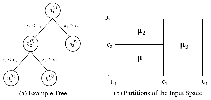
Figure 2: (Left) An example of a tree structure $T$ applied to a $2$-dimensional input space. The internal and terminal nodes of the tree are denoted with superscripts $(i)$ and $(t)$, respectively. Each internal node facilitates a binary split of the form $x_{v}<c_{v}$. (Right) The partitions of the rectangular input space $[L_{1},U_{1}]\times[L_{2},U_{2}]$, with associated terminal node parameters $\mu_{b}$, $b=1,2,3$. The function $g(\boldsymbol{x};T,M)$ maps a given $\boldsymbol{x}$ to one of these three values.

The tree topology prior, $\pi(T)$, accounts for the type of each node within the tree (terminal or internal) along with the splitting rules selected at each internal node. The default prior is uninformative for the split rules and penalizes tree depth (Chipman et al., 2010). For example, the probability that a node $\eta$ is internal is given as $\pi(\eta\text{ is internal})=\alpha(1+d_{\eta})^{-\beta}$, where $\alpha$ and $\beta$ are tuning parameters and $d_{\eta}$ denotes the depth of $\eta$. The output of the tree corresponds to the set of the terminal node parameters $M$. In most cases, a conjugate normal prior is assigned to each of the terminal node parameters $\mu_{1},\ldots,\mu_{B}$. Another common assumption is that the terminal node parameters are conditionally independent given the tree topology $T$. These assumptions simplify the Markov Chain Monte Carlo (MCMC), particularly when working with a Gaussian likelihood. Specifically, the conjugacy avoids the need for a complex Reversible Jump MCMC.

Given data and the specified prior distributions, samples from the posterior of $T,\ M$ and $\sigma^{2}$ are generated using MCMC. The tree topology is updated at each iteration by proposing a slight change to the existing tree structure (Chipman et al., 1998; Pratola, 2016). The terminal node and variance parameters are then updated using Gibbs sampling steps.

The methodology outlined above is easily extended to an ensemble of $m$ trees, $T_{1},\ldots,T_{m},$ with terminal node parameter sets $M_{1},\ldots,M_{m}$ (Chipman et al., 2010) using a Bayesian backfitting algorithm (Hastie and Tibshirani, 2000). The mean function becomes

$$E[Y(\boldsymbol{x})\mid\boldsymbol{x}] =\sum_{j=1}^{m}g(\boldsymbol{x};T_{j},M_{j}),$$ (1)

where $g(\boldsymbol{x};T_{j},M_{j})=\sum_{b=1}^{B_{j}}\mu_{bj}\;I(\boldsymbol{x}\in\mathcal{X}_{bj})$ and $I(\boldsymbol{x}\in\mathcal{X}_{bj})$ is an indicator function denoting the event that $\boldsymbol{x}$ is mapped to the $b\text{th}$ partition of the input space by tree $j$.

Generally, tree models result in a piecewise constant mean function. When continuity is desirable, soft regression trees (Irsoy et al., 2012; Linero and Yang, 2018) can serve as a useful alternative. A soft regression tree maps an observation with input $\boldsymbol{x}$ to a unique terminal node probabilistically given the tree topology and associated splitting rules. If $T_{j}$ has $B_{j}$ terminal nodes, the probability of being mapped to the $b\text{th}$ terminal node is given by $\phi_{bj}(\boldsymbol{x};T_{j},\gamma_{j})$ for $b=1,\ldots,B_{j}$ and bandwidth parameter $\gamma_{j}$. The bandwidth parameter is used to control the amount of smoothing across the terminal node parameters. Given each input dimension is standardized so that $x_{v}\in[0,1]$, SBART assumes $\gamma_{j}$ to be exponentially distributed with a mean of $0.1$. Larger values of $\gamma_{j}$ ($\geq 0.1$) will lead to a more global solution, while small values of $\gamma_{j}$ tends to generate a localized fit similar to BART. The mean function of a soft regression tree is then constructed as a weighted average of the terminal node parameters

$$g(\boldsymbol{x};T_{j},M_{j})=\sum_{b=1}^{B_{j}}\mu_{bj}\;\phi_{bj}(\boldsymbol{x};T_{j},\gamma_{j}).$$ (2)

Once more, the traditional regression tree with deterministic paths can be thought of as a special case where $\phi_{bj}(\boldsymbol{x};T_{j},\gamma_{j})=I(\boldsymbol{x}\in\mathcal{X}_{bj}).$

This expression for the mean function requires the terminal node parameters to be updated jointly during the MCMC. When the terminal node parameters are scalars, this requires inversion of a non-sparse $B_{j}\times B_{j}$ matrix (Linero and Yang, 2018). In most cases, the trees are regularized to maintain a shallow depth, so this inversion is relatively inexpensive to compute. If the terminal node parameters are $K$-dimensional vectors, the corresponding update requires inversion of a $KB_{j}\times KB_{j}$ matrix, which can quickly become computationally expensive even with shallow trees. Climate applications typically involve large amounts of data and thus we can expect deeper trees will be required to combine a set of GCMs. The proposed Random Path BART (RPBART) model described next alleviates these concerns.

3 The Random Path Model

We first propose our smooth, continuous, Random Path model for standard BART (RPBART), which models a univariate mean function. Let $Y(\boldsymbol{x}_{i})$ be an observable quantity from some unknown process at input $\boldsymbol{x}_{i}$. Let $z_{bj}(\boldsymbol{x}_{i})$ be the latent random path indicator for the event that the $i\text{th}$ input is mapped to the $b\text{th}$ terminal node in $T_{j}$. Given the random path assignments, we assume $Y(\boldsymbol{x}_{i})$ is modeled as

$$Y(\boldsymbol{x}_{i})\mid\{T_{j},M_{j},Z_{j}\}_{j=1}^{m},\sigma^{2}\; \sim\;N\Big{(}\sum_{j=1}^{m}g(\boldsymbol{x}_{i};T_{j},M_{j},Z_{j}),\sigma^{2}\Big{)},$$ (3)

$$g(\boldsymbol{x}_{i};T_{j},M_{j},Z_{j}) =\sum_{b=1}^{B_{j}}\mu_{bj}\;z_{bj}(\boldsymbol{x}_{i}).$$ (4)

Each observation is mapped to exactly one terminal node within $T_{j}$, thus $\sum_{b=1}^{B_{j}}z_{bj}(\boldsymbol{x}_{i})=1$ and $z_{bj}(\boldsymbol{x}_{i})\in\{0,1\}$ for $b=1,\ldots,B_{j}$ and $i=1,\ldots,n$. The set $Z_{j}$ is then defined as $Z_{j}=\{\boldsymbol{z}_{j}(\boldsymbol{x}_{i})\}_{i=1}^{n}$ where $\boldsymbol{z}_{j}(\boldsymbol{x}_{i})$ is the $B_{j}$-dimensional vector of random path assignments for the $i\text{th}$ input. Traditional BART with deterministic paths can be viewed as a special case of RPBART where $z_{bj}(\boldsymbol{x}_{i})=I(\boldsymbol{x}_{i}\in\mathcal{X}_{bj})$. Conditional on $Z_{j}$, the output of the random path tree remains a piecewise constant form. However, taking the expectation of the sum-of-trees with respect to $Z_{j}$ results in a continuous function, similar to SBART (2).

3.1 Prior Specification

The original BART model depends on the tree structures, associated set of terminal node parameters, and error variance. We maintain the usual priors for each of these components,

$$\mu_{bj}\mid T_{j} \sim N(0,\tau^{2}),\quad T_{j}\sim\pi(T_{j}),\quad\sigma^{2}\sim\nu\lambda/\chi^{2}_{\nu},$$

where $b=1,\ldots,B_{j}$ and $j=1,\ldots,m$. The values of $\tau$, $\lambda$, and $\nu$ can still be selected using similar methods as specified by Chipman et al. (2010).

RPBART introduces two new sets of parameters, $(Z_{j},\gamma_{j})$ for $j=1,\ldots,m$. For each $Z_{j}$, consider the path assignment for the $i\text{th}$ observation, $\boldsymbol{z}_{j}(\boldsymbol{x}_{i})$. Conditional on $T_{j}$, the $B_{j}$-dimensional random path vector for a given $\boldsymbol{x}_{i}$ is assigned a Multinomial prior

$$\boldsymbol{z}_{j}(\boldsymbol{x}_{i})\mid T_{j},\gamma_{j}\sim\text{Multinomial}\Big{(}1;\phi_{1j}(\boldsymbol{x}_{i};T_{j},\gamma_{j}),\ldots,\phi_{{B_{j}}j}(\boldsymbol{x}_{i};T_{j},\gamma_{j})\Big{)},$$ (5)

where $\phi_{bj}(\boldsymbol{x}_{i};T_{j},\gamma_{j})$ is the probability an observation with input $\boldsymbol{x}_{i}$ is mapped to the $b\text{th}$ terminal node in $T_{j}$ or equivalently, the conditional probability that $z_{bj}(\boldsymbol{x}_{i})=1$. The bandwidth parameter, $\gamma_{j}$, takes values within the interval $(0,1)$ and controls the degree of pooling across terminal nodes. As $\gamma_{j}$ increases, more information is shared across the terminal nodes, which leads to a less localized prediction. Since we confine $\gamma_{j}$ to the interval $(0,1)$, we assume

$$\gamma_{j}\sim\text{Beta}(\alpha_{1},\alpha_{2}),\quad j=1,\ldots,m.$$

This prior specification of $\gamma_{j}$ noticeably differs from the exponential bandwidth prior used in SBART (Linero and Yang, 2018). The different modeling assumptions are guided by the design of the path probabilities, $\phi_{bj}(\boldsymbol{x}_{i};T_{j},\gamma_{j})$, which are discussed in Section 3.2.

Finally, we assume conditional independence given the set of $m$ trees. This implies the joint prior simplifies as

$$\pi\big{(}\sigma^{2},\{T_{j},M_{j},Z_{j},\gamma_{j}\}_{j=1}^{m}\big{)} =\pi(\sigma^{2})\prod_{j=1}^{m}\pi(M_{j}\mid T_{j},Z_{j})\;\pi(Z_{j}\mid T_{j},\gamma_{j})\;\pi(T_{j})\pi(\gamma_{j})$$

$$=\pi(\sigma^{2})\prod_{j=1}^{m}\pi(T_{j})\;\pi(\gamma_{j})\prod_{b=1}^{B_{j}}\pi(\boldsymbol{\mu}_{bj}\mid T_{j})\;\pi(Z_{j}\mid T_{j},\gamma_{j}).$$ (6)

Furthermore, we assume mutual independence across the random path assignment vectors $\boldsymbol{z}_{j}(\boldsymbol{x}_{i})$ apriori. Thus the set of vectors over the $n$ training points can be rewritten as

$$\pi(Z_{j}\mid T_{j},\gamma_{j})=\prod_{i=1}^{n}\prod_{b=1}^{B_{j}}\Big{(}\phi_{bj}(\boldsymbol{x}_{i};T_{j},\gamma_{j})\Big{)}^{z_{bj}(\boldsymbol{x}_{i})}.$$ (7)

3.2 The Path Probabilities

The continuity in the mean prediction from each tree is driven by the $B_{j}$ path probabilities, $\phi_{bj}(\boldsymbol{x}_{i};T_{j},\gamma_{j})$. Recall, a tree model recursively partitions the input space into $B_{j}$ disjoint subregions using a sequence of splitting rules. We define the path from the root node, $\eta_{1j}^{(i)}$, to the $b\text{th}$ terminal node, $\eta_{bj}^{(t)}$, in terms of the sequence of internal nodes that connect $\eta_{1j}^{(i)}$ and $\eta_{bj}^{(t)}$. To define $\phi_{bj}(\boldsymbol{x}_{i};T_{j},\gamma_{j})$, we must consider the probability of visiting the internal nodes that form the path that connects $\eta_{1j}^{(i)}$ and $\eta_{bj}^{(t)}$.

For example, consider the tree with $B_{j}=3$ terminal nodes (red, blue, green) and induced partition of the $1$-dimensional input space, $[-1,1]$, in Figure 4. In this tree, the path to the red terminal node, $\eta_{1j}^{(t)}$, is simply defined by splitting left at the root node. Similarly, the path to the blue terminal node, $\eta_{2j}^{(t)}$, is defined by first splitting right at $\eta_{1j}^{(i)}$ and then left at $\eta_{2j}^{(i)}$. In the usual regression tree model, these splits happen deterministically. This means an observation with $x_{1}<0$ splits left and is thus mapped to $\eta_{1j}^{(t)}$ with probability 1. Using our random path model, an observation splits right with probability $\psi(\boldsymbol{x};\cdot)$ and left with probability $1-\psi(\boldsymbol{x};\cdot)$. This adds another layer of stochasticity into the model.

3.2.1 Defining the Splitting Probabilities

Consider the $d\text{th}$ internal node, $\eta^{(i)}_{dj}$, of $T_{j}$. Assume $\eta^{(i)}_{dj}$ splits on the rule $x_{v_{(dj)}}<c_{(dj)}$. Let $\psi(\boldsymbol{x};v_{(dj)},c_{(dj)},\gamma_{j})$ define the probability an observation with input $\boldsymbol{x}$ moves to the right child of $\eta^{(i)}_{dj}$. Further assume the cutpoint $c_{(dj)}$ is selected from the discretized subset $(L^{d}_{v},U^{d}_{v})\cap\mathcal{C}_{v}$, where $\mathcal{C}_{v}$ is the finite set of possible cutpoints for variable $v$, and $L^{d}_{v}$ and $U^{d}_{v}$ are the upper and lower bounds defined based on the previous splitting rules in the tree. The bounds, which are computed based on the information in $T_{j}$, are used to define a threshold which establishes a notion of “closeness” between points. We incorporate this information into the definition of $\psi(\boldsymbol{x};v_{(dj)},c_{(dj)},\gamma_{j})$ by

$$\psi(\boldsymbol{x};v_{(dj)},c_{(dj)},\gamma_{j})=\begin{cases}1-\frac{1}{2}\Big{(}1-\frac{x_{v_{(dj)}}-c_{(dj)}}{\gamma_{j}(U^{d}_{v}-c_{(dj)})}\Big{)}^{q}_{+}&x_{v_{(dj)}}\geq c_{(dj)},\\[7.0pt] \frac{1}{2}\Big{(}1-\frac{c_{(dj)}-x_{v_{(dj)}}}{\gamma_{j}(c_{(dj)}-L^{d}_{v})}\Big{)}^{q}_{+}&x_{v_{(dj)}}<c_{(dj)},\end{cases}$$ (8)

where the expression $a_{+}=\max\{a,0\}$ for any $a\in\mathbb{R}$ and $q$ is a shape parameter. This definition of $\psi(\boldsymbol{x};v_{(dj)},c_{(dj)},\gamma_{j})$ restricts the probabilistic assignment to the left or right child of $\eta^{(i)}_{dj}$ to the interval $\mathcal{I}_{dj}(\gamma_{j}):=\big{(}c_{(dj)}-\gamma_{j}(c_{(dj)}-L^{d}_{v}),\;c_{(dj)}+\gamma_{j}(U^{d}_{v}-c_{(dj)}))$. Any observation with input $x_{v_{(dj)}}$ such that $x_{v_{(dj)}}\in\mathcal{I}_{dj}(\gamma_{j})$ has a non-zero chance of being assigned to either of the child nodes in the binary split. Meanwhile, $\psi(\boldsymbol{x};v_{(dj)},c_{(dj)},\gamma_{j})=0$ if $x_{v_{(dj)}}$ is less than the lower bound in $\mathcal{I}_{dj}(\gamma_{j})$ or $\psi(\boldsymbol{x};v_{(dj)},c_{(dj)},\gamma_{j})=1$ if $x_{v_{(dj)}}$ is greater than the upper bound in $\mathcal{I}_{dj}(\gamma_{j})$. This means the probabilistic assignment agrees with the deterministic split when $x_{v_{(dj)}}\notin\mathcal{I}_{dj}(\gamma_{j})$. In other words, points that are farther away from the cutpoint take the deterministic left or right move while points close to the cutpoint take a random move left or right.

To understand $\gamma_{j}$, consider the first split (at the root node) within a given a tree. Assume the root node splits the interval $[L_{1}^{(1)},U_{1}^{(1)}]=[-1,1]$ using the rule $x_{1}<0$ (i.e. $v_{1j}=1$ and $c_{1j}=0$). Figure 3 displays the probability of splitting left (red), $1-\psi(\boldsymbol{x};1,0,\gamma_{j})$, and the probability of splitting right (blue), $\psi(\boldsymbol{x};1,0,\gamma_{j})$, for different values of $\gamma_{j}$ as a function of $x_{1}$. The orange region in each panel highlights the set $\mathcal{I}_{1j}(\gamma_{j})$. The interval is wider for larger $\gamma_{j}$, which means a larger proportion of points can move to the left or right child nodes. As $\gamma_{j}$ decreases, the probability curves become steeper and $\psi(\boldsymbol{x};1,0,\gamma_{j})$ starts to resemble the deterministic rule $I(x_{v_{(dj)}}\geq c_{(dj)})$.

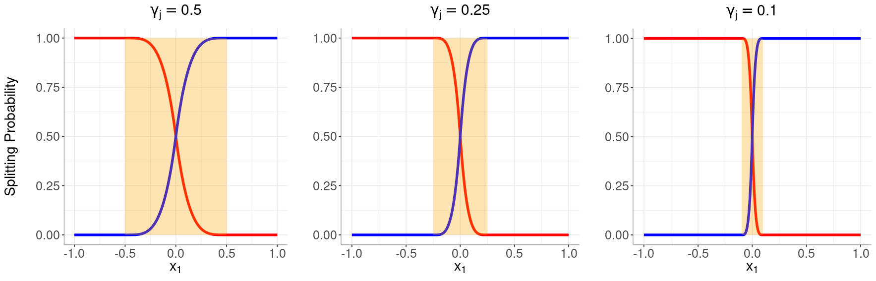
Figure 3: Three examples of $1-\psi(\boldsymbol{x};1,0,\gamma_{j})$ (red) and $\psi(\boldsymbol{x};1,0,\gamma_{j})$ (blue) with bandwidth parameters of $0.5$, $0.25$, and $0.1$, corresponding to the move that splits the interval $[L^{(1)}_{1},U^{(1)}_{1}]=[-1,1]$ on the cutpoint $c_{1j}=0$. The interval $\mathcal{I}_{1j}(\gamma_{j})$ (orange) defines the interval where the random path assignment can disagree with the traditional deterministic path assignment.

The splitting probabilities determine how to traverse the tree along the various paths created by the internal nodes. These probabilities set the foundation for computing the probability of reaching any of the $B_{j}$ terminal nodes within $T_{j}$.

3.2.2 Defining the Path Probabilities

The path probabilities, $\phi_{bj}(\boldsymbol{x};T_{j},\gamma_{j})$, can be defined in terms of the individual splits at each internal node. For example, consider the tree with $B_{j}=3$ terminal nodes in Figure 4. The first internal node, $\eta_{1j}^{(i)}$, splits using $v_{1j}=1$ and $c_{1j}=0$, while the second internal node, $\eta_{2j}^{(i)}$, splits using $v_{2j}=1$ and $c_{2j}=0.4$. The probability of reaching the red terminal node is simply the probability of splitting left at $\eta_{1j}^{(i)}$, which is given by $\phi_{1j}(\boldsymbol{x};T_{j},\gamma_{j})=1-\psi(\boldsymbol{x};1,0,\gamma_{j}).$ Meanwhile, an observation is mapped to the blue terminal node by first splitting right at $\eta_{1j}^{(i)}$ and then left at $\eta_{2j}^{(i)}$. This sequence of moves occurs with probability $\phi_{2j}(\boldsymbol{x};T_{j},\gamma_{j})=\psi(\boldsymbol{x};1,0,\gamma_{j})\times\Big{(}1-\psi(\boldsymbol{x};1,0.4,\gamma_{j})\Big{)}.$ The resulting path probabilities for each terminal node with $\gamma_{j}=0.5$ are shown in the right panel of Figure 4.

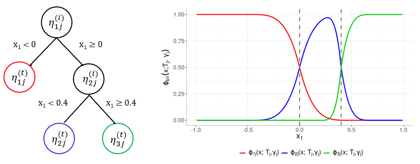
Figure 4: (Left) An example tree with $B_{j}=3$ terminal nodes (red, blue, green). The internal nodes (black) define a set of splitting rules that recursively partition the input space. (Right) Example path probabilities, $\phi_{bj}(\boldsymbol{x};T_{j},\gamma_{j})$, using $\gamma_{j}=0.5$. Each curve displays the probability of being mapped to the terminal node of the same color as a function of $x_{1}$. For example, an observation with $x_{1}=0$ has a probability of 0.5 of being mapped to the red terminal node and a probability of 0.5 of being mapped to the blue terminal node.

In general, if the path from the root node to the $b\text{th}$ terminal node depends on $D$ internal nodes, the path probability is defined by

$$\phi_{bj}(\boldsymbol{x};T_{j},\gamma_{j})=\prod_{d=1}^{D}\psi(\boldsymbol{x};v_{(dj)},c_{(dj)},\gamma_{j})^{R_{(dj)}}\times\big{(}1-\psi(\boldsymbol{x};v_{(dj)},c_{(dj)},\gamma_{j})\big{)}^{1-R_{(dj)}},$$ (9)

where $v_{(dj)}$ and $c_{(dj)}$ are the variable and cutpoint selected at the $d\text{th}$ internal node along the specified path in $T_{j}$, and $R_{(dj)}=1$ ($R_{(dj)}=0$) if a right (left) move is required at the $d\text{th}$ internal node to continue along the path towards $\eta^{(t)}_{bj}$.

3.3 Smooth Mean Predictions

Let $Y(\tilde{\boldsymbol{x}})$ be a new observable quantity at input $\tilde{\boldsymbol{x}}$. Conditional on the $m$ random path vectors at $\tilde{x}$, the mean function is given by

$$E[Y(\tilde{\boldsymbol{x}})\mid\{T_{j},M_{j},\tilde{Z}_{j},\gamma_{j}\}_{j=1}^{m}] =\sum_{j=1}^{m}\boldsymbol{g}(\tilde{\boldsymbol{x}};T_{j},M_{j},\tilde{Z}_{j})$$

$$=\sum_{j=1}^{m}\sum_{b=1}^{B_{j}}\boldsymbol{\mu}_{bj}\;z_{bj}(\tilde{\boldsymbol{x}}),$$

where $\tilde{Z}_{j}=Z_{j}\cup\{\boldsymbol{z}_{j}(\tilde{\boldsymbol{x}})\}$ is the set of random path assignments from the training data and the future observation. Marginalizing over the random path assignments results in a smooth mean prediction,

$$E[Y(\tilde{\boldsymbol{x}})\mid\{T_{j},M_{j},\gamma_{j}\}_{j=1}^{m}] =\sum_{j=1}^{m}\sum_{b=1}^{B_{j}}\boldsymbol{\mu}_{bj}\;\phi_{bj}(\tilde{\boldsymbol{x}};T_{j},\gamma_{j}).$$ (10)

Posterior samples of this expectation can be obtained by evaluating the functional form in (10) given posterior draws of $T_{j}$, $M_{j}$, and $\gamma_{j}$.

3.4 The Semivariogram

The RPBART model introduces an additional pair of hyperparameters, $\alpha_{1}$ and $\alpha_{2}$, which control the $m$ bandwidth parameters $\gamma_{j},$ and therefore the level of smoothing in the model. The common approach in BART is to calibrate the prior hyperparameters using a lightly data-informed approach or cross validation. However, neither the data-informed approach proposed for BART (Chipman et al., 2010) nor the default prior settings in SBART (Linero and Yang, 2018) can be used for calibrating the new smoothness parameters $\alpha_{1}$ and $\alpha_{2}$. Furthermore, the added complexity of RPBART would render the traditional cross-validation study too complex and computationally expensive. Thus, we propose to calibrate RPBART using the semivariogram (Cressie, 2015).

The semivariogram, $\overline{\nu}(\lVert\boldsymbol{h}\rVert)$, is defined by

$$\overline{\nu}(\lVert\boldsymbol{h}\rVert)=\frac{1}{|\mathcal{X}|}\int_{\mathcal{X}}\nu(\boldsymbol{x},\boldsymbol{h})\;d\boldsymbol{x},$$ (11)

$$\nu(\boldsymbol{x},\boldsymbol{h})=\frac{1}{2}\text{Var}\big{(}Y(\boldsymbol{x}+\boldsymbol{h})-Y(\boldsymbol{x})\big{)},$$ (12)

where $|\mathcal{X}|$ denotes the volume of the input domain $\mathcal{X}$ and $\boldsymbol{x}+\boldsymbol{h}$ denotes an input which is a distance $\lVert\boldsymbol{h}\rVert>0$ away from $\boldsymbol{x}$ (Matheron, 1963). Assuming a constant mean function for $Y(\boldsymbol{x})$, the function $\nu(\boldsymbol{x},\boldsymbol{h})$ simplifies as

$$\nu(\boldsymbol{x},\boldsymbol{h})=\frac{1}{2}E\Big{[}\big{(}Y(\boldsymbol{x}+\boldsymbol{h})-Y(\boldsymbol{x})\big{)}^{2}\Big{]}.$$ (13)

In spatial statistics, the function $\nu(\boldsymbol{x},\boldsymbol{h})$ describes the spatial correlation between two points that are separated by a distance of $\lVert\boldsymbol{h}\rVert$ and may depend on parameters that determine the shape of the semivariogram $\overline{\nu}(\lVert\boldsymbol{h}\rVert)$.

We propose calibrating the hyperparameters of the RPBART model by using an estimator of the prior semivariogram in (11) and the function $\nu(\boldsymbol{x},\boldsymbol{h})$ in (12). The estimator of (12) can be can be calculated by marginalizing over the set of parameters $\{T_{j},M_{j},Z_{j},\gamma_{j}\}_{j=1}^{m}$ and conditioning on $\sigma^{2}$. In order to compute $\nu(\boldsymbol{x},\boldsymbol{h})$, we first analytically marginalize over $\{M_{j},Z_{j}\}_{j=1}^{m}$ conditional on the remaining parameters. An expression for $\nu(\boldsymbol{x},\boldsymbol{h})$ is then computed by numerically integrating over $\{T_{j},\gamma_{j}\}_{j=1}^{m}$ (where $\sigma^{2}$ is held fixed). The function $\nu(\boldsymbol{x},\boldsymbol{h})$ for the RPBART model is given by Theorem 3.1.

Theorem 3.1.

Assume the random quantities $\{T_{j},M_{j},Z_{j},\gamma_{j}\}_{j=1}^{m}$ are distributed according to prior specification in Section 3.1. Conditional on $\sigma^{2}$, the function $\nu(\boldsymbol{x},\boldsymbol{h})$ for the RPBART model is

$$\nu(\boldsymbol{x},\boldsymbol{h}) =\sigma^{2}+m\tau^{2}\Big{(}1-\bar{\Phi}(\boldsymbol{x},\boldsymbol{h})\Big{)},$$ (14)

where $m\tau^{2}=\Big{(}\frac{y_{\text{max}}-y_{\text{min}}}{2k}\Big{)}^{2}$ defines the variance of the sum-of-trees, $k$ is a tuning parameter, $y_{\text{max}}-y_{\text{min}}$ is the range of the observed data, and

$$\bar{\Phi}(\boldsymbol{x},\boldsymbol{h})=E\Big{[}\sum_{b=1}^{B_{1}}\phi_{b1}(\boldsymbol{x}+\boldsymbol{h};\gamma_{1},T_{1})\phi_{b1}(\boldsymbol{x};\gamma_{1},T_{1})\Big{]},$$

is the probability two observations with inputs $\boldsymbol{x}$ and $\boldsymbol{x}+\boldsymbol{h}$ are assigned to the same partition. Without loss of generality the expectation is with respect to $T_{1}$, and $\gamma_{1}$ (since the $m$ trees are a priori i.i.d.).

The proof of Theorem 3.1 is in Section 8.2 of the Supplement. The expectation, $\bar{\Phi}(\boldsymbol{x},\boldsymbol{h})$, in Theorem 3.1 can be approximated using draws from the prior. This expression shows that $\nu(\boldsymbol{x},\boldsymbol{h})$ depends on the probability that two points are assigned to different partitions, averaged over the set of trees and bandwidth parameters, as denoted by $1-\bar{\Phi}(\boldsymbol{x},\boldsymbol{h})$. This probability is then scaled and shifted by the variance of the sum-of-trees, $m\tau^{2}$, and error variance, $\sigma^{2}$.

Generally, we are more interested in $\overline{\nu}(\lVert\boldsymbol{h}\rVert)$, which describes the variability across the entire input space rather than at a specific $\boldsymbol{x}$. For RPBART, we can numerically compute $\overline{\nu}(\lVert\boldsymbol{h}\rVert)$ by integrating (14) over $\mathcal{X}$ as shown in (11). We can use the resulting a priori semivariogram estimator to guide the selection of the hyperparameters, $\alpha$, $\beta$, $\alpha_{1}$, $\alpha_{2}$, and $k$, across the various priors in the model. Note the number of trees $m$ must still be selected through other means, such as cross-validation.

We note this procedure for computing the semivariogram is more complex than what is observed with Gaussian Processes (Cressie, 2015). In such cases, shift-invariant kernels are typically selected for the covariance model in a stationary Gaussian Process. In other words, the covariance model is simply a function of $\boldsymbol{h}$ under a shift-invariant kernel. However, in the RPBART model, the covariance function, $\bar{\Phi}(\boldsymbol{x},\boldsymbol{h})$ is a non-shift-invariant product kernel of the path probabilities that is averaged over all possible trees and bandwidth parameters. Because of this, we must carefully consider the computation of $\nu(\boldsymbol{x},\boldsymbol{h})$ in order to numerically compute $\overline{\nu}(\lVert\boldsymbol{h}\rVert)$.

For example, consider the semivariogram with respect to the 2-dimensional input space $[-1,1]\times[-1,1]$. Figure 5 displays possible semivariograms for different values of $k$, $\alpha_{1}$, and $\alpha_{2}$ with $y_{min}=-1$ and $y_{max}=1$. Note, we set the nugget $\sigma=0$ in this Figure to clearly isolate the effect of the smoothness parameters $\alpha_{1}$ and $\alpha_{2}$, i.e. ignoring the nugget. Each panel corresponds to different settings of the bandwidth prior, where $\alpha_{1}=2$ and $\alpha_{2}=25$ indicate low levels of smoothing and $\alpha_{1}=15$ and $\alpha_{2}=10$ indicate high levels of smoothing. Based on each curve, we see the smoothing parameters primarily affect the behavior of the semivariogram for small values of $\lVert\boldsymbol{h}\rVert$. In the low smoothing case (left), each of the semivariograms take values closer to $0$ when $\lVert\boldsymbol{h}\rVert$ is small, while a noticeable shift upwards is observed in the higher smoothing cases (center and right). This offset behavior appears in the RPBART semivariogram regardless of the bandwidth hyperparameters because the covariance function is discontinuous.

As $\lVert\boldsymbol{h}\rVert$ increases, each semivariogram reaches a maximum value, known as the sill. For each $k$, we observe the sill is similar regardless of the values of $\alpha_{1}$ and $\alpha_{2}$. Thus, the value of $k$ controls the height of the sill and in turn the amount of variability attributed to the sum-of-trees model. As a result, the interpretation of $k$ under the RPBART model is the same as in the original BART model. Finally, we should note that the hyperparameters in the tree prior, $\alpha$ and $\beta$, can also be determined based on the semivariogram, as deeper trees result in a larger number of partitions and thus less correlation across the input space. Hence, deeper trees tend to shift the semivariograms upwards and further contribute to the offset.

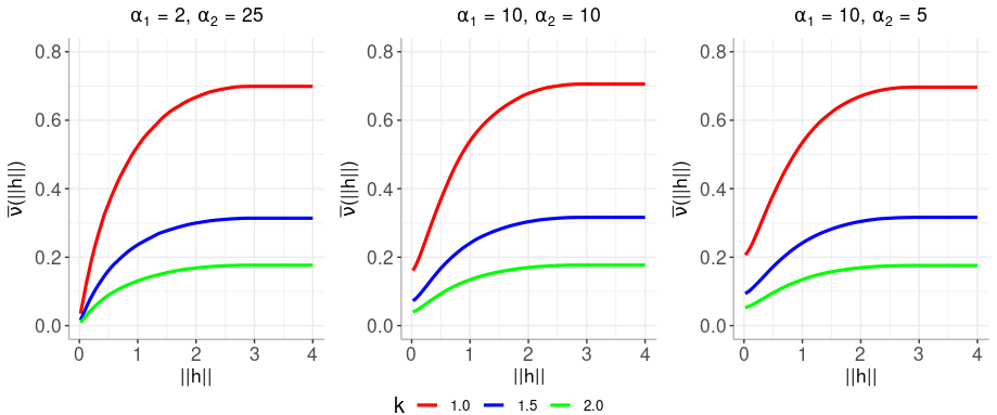
Figure 5: The semivariogram for different values of $k=1$ (red), $k=1.5$ (blue), and $k=2$ (green) and bandwidth hyperparameters $\alpha_{1}$ and $\alpha_{2}$. Each semivariogram is generated using $y_{min}=-1$, $y_{max}=1$, $\sigma=0$, and $\alpha=0.95$, and $\beta=0.5$.

In practice, we can compare the theoretical semivariogram to the empirical semivariogram to select the hyperparameters for the model (Cressie, 2015). In summary, we see $\alpha_{1}$ and $\alpha_{2}$ primarily affect the semivariogram when $\lVert\boldsymbol{h}\rVert$ is near $0$, as more smoothing generally leads to an upward shift and increase in curvature near the origin. The tree prior hyperparameters, $\alpha$ and $\beta$, affect the size of the offset and the height of the sill. Meanwhile, the value of $k$ simply scales the function and has minimal impact on the overall shape of the curve.

The last component to consider is the value of $\sigma^{2}$, which is set to $0$ in Figure 5. The typical way to calibrate the $\nu\lambda/\chi_{\nu}^{2}$ prior on $\sigma^{2}$ is to fix $\nu$ at a desired value and select $\lambda$ based on an estimate of $\sigma^{2}$, denoted by $\hat{\sigma}^{2}$ (Chipman et al., 2010; Linero and Yang, 2018). Traditional approaches typically compute $\hat{\sigma}^{2}$ using a linear model. From Theorem 3.1, we see $\sigma^{2}$ simply adds to the offset by vertically shifting the semivariogram. Thus, we can select $\hat{\sigma}^{2}$ based on theoretical and empirical semivariogram. Given a fixed value of $\nu$ (usually around 10), one can set $\hat{\sigma}^{2}$ to be the mode of the prior distribution and algebraically solve for the scale parameter $\lambda$. This strategy allows us to select $\lambda$, along with the other hyperparameters, using the same information encoded in the semivariogram.

4 Smooth Model Mixing

4.1 A Mean-Mixing Approach

The RPBART model can be easily extended to the BART-based model mixing framework originally presented by Yannotty et al. (2024). Let $f_{1}(\boldsymbol{x}_{i}),\ldots,f_{K}(\boldsymbol{x}_{i})$ denote the output from $K$ simulators at an input $\boldsymbol{x}_{i}$. When the simulators are computationally expensive, the output $f_{l}(\boldsymbol{x}_{i})$ is replaced with the prediction from an inexpensive emulator, $\hat{f}_{l}(\boldsymbol{x}_{i})$, for $l=1,\ldots,K$. For example, $\hat{f}_{l}(\boldsymbol{x}_{i})$ could be the mean prediction from a Gaussian process emulator (Santner et al., 2018) or an RPBART emulator. In climate applications, each GCM may be evaluated on different latitude and longitude grids, thus we use regridding techniques such as bilinear interpolation to compute $\hat{f}_{l}(\boldsymbol{x}_{i})$.

Given the mean predictions from $K$ emulators, we assume $Y(\boldsymbol{x}_{i})$ is modeled by

$$Y(\boldsymbol{x}_{i})\mid\boldsymbol{\hat{f}}(\boldsymbol{x}_{i}),\{T_{j},M_{j},Z_{j}\}_{j=1}^{m},\sigma^{2}\; \sim\;N\big{(}\boldsymbol{\hat{f}}^{\top}(\boldsymbol{x}_{i})\boldsymbol{w}(\boldsymbol{x}_{i}),\sigma^{2}),$$

$$\boldsymbol{w}(\boldsymbol{x}_{i}) =\sum_{j=1}^{m}\boldsymbol{g}(\boldsymbol{x}_{i};T_{j},M_{j},Z_{j}),$$

$$\boldsymbol{g}(\boldsymbol{x};T_{j},M_{j},Z_{j}) =\sum_{b=1}^{B_{j}}\boldsymbol{\mu}_{bj}z_{bj}(\boldsymbol{x}_{i}),$$

where $\boldsymbol{\hat{f}}(\boldsymbol{x}_{i})$ is the $K$-dimensional vector of mean predictions at input $\boldsymbol{x}_{i}$, $\boldsymbol{w}(\boldsymbol{x}_{i})$ is the corresponding $K$-dimensional weight vector, and $i=1,\ldots,n$. This extension allows the $K$ weights to be modeled as continuous functions using similar arguments as outlined for the 1-dimensional tree output case in Section 3.3.

Similar to Yannotty et al. (2024), we regularize the weight functions via a prior on the terminal node parameters. The primary goal is to ensure each weight function, $w_{l}(\boldsymbol{x})$, prefers the interval $[0,1]$ without directly imposing a strict non-negativity or sum-to-one constraint. Thus, we assume

$$\boldsymbol{\mu}_{bj}\mid T_{j}\sim N\Big{(}\frac{1}{mK}\boldsymbol{1}_{K}\;,\tau^{2}I_{K}\Big{)},$$ (15)

where $\tau=1/(2k\sqrt{m})$ and $k$ is a tuning parameter. This choice of $\tau$ follows Chipman et al. (2010) in that the confidence interval for the sum-of-trees has a length of $w_{max}-w_{min}$, where 0 and 1 are the target minimum and maximum values of the weights. This prior calibration ensures each $w_{l}(\boldsymbol{x})$ is centered about $1/K$, implying each model is equally weighted at each $\boldsymbol{x}$ apriori. The value of $k$ controls the flexibility of the weight functions. Small $k$ allows for flexible weights that can vary easily beyond the target bounds of $0$ and $1$ and thus are able to identify granular patterns in the data. Larger $k$ will keep the weights near the simple average of $1/K$ and could be limited in identifying regional patterns in the data. Typically, more flexible weights are needed when mixing lower fidelity or lower resolution models, as the weights will account for any discrepancy between the model set and the observed data. By default, we set $k=1$.

RPBART allows for independent sampling of each of the $B_{j}$ terminal node parameters, $\boldsymbol{\mu}_{bj}$, within $T_{j}$ for $j=1,\ldots,m$. As previously discussed, this avoids the joint update required in SBART. This is rather significant, as the SBART update for the $B_{j}$ terminal node parameters vectors would require an inversion of a $KB_{j}\times KB_{j}$ matrix. In larger scale problems with larger $K$ or deeper trees, the repeated inversion cost of this matrix would be burdensome.

4.2 The Semivariogram

To calibrate the remaining hyperparameters of our RPBART-based mixing model, we employ the prior semivariogram introduced in Section 3.4. The semivariogram of Theorem 3.1 can be extended to the model mixing framework by considering the assumptions associated with each emulator. One cannot directly apply the results conditional on the point estimates of each emulator, $\hat{f}_{1}(\boldsymbol{x}),\ldots,\hat{f}_{K}(\boldsymbol{x})$, because the semivariogram is designed to assess the spatial variability of the model free of any mean trend (Gringarten and Deutsch, 2001).

Rather than condition on the model predictions, we treat each of the individual emulators $f_{1}(\boldsymbol{x}),\ldots,f_{K}(\boldsymbol{x})$ as unknown quantities. Thus, the semivariogram for $Y(\boldsymbol{x})$ will assess the modeling choices for the sum-of-trees mixing model along with modeling choices for each $f_{l}(\boldsymbol{x})$. For example, we might assume GP emulators,

$$f_{l}(\boldsymbol{x})\mid\boldsymbol{\psi}_{l}\;\sim\text{GP}\big{(}\bar{f}_{l},\;R_{l}(\boldsymbol{x},\boldsymbol{x}^{\prime};\boldsymbol{\psi}_{l})\big{)},$$

where $\boldsymbol{\psi}_{l}$ is a vector of parameters such as the scale or length scale and $\bar{f}_{l}$ is a constant mean.

Theorem 4.1.

Assume the random quantities $\{T_{j},M_{j},Z_{j},\gamma_{j}\}_{j=1}^{m}$ are distributed according to prior specification in Section 3.1. Assume each simulator is modeled as a stochastic emulator with mean $\bar{f}_{l}$ and covariance kernel $R_{l}({\boldsymbol{x}},\boldsymbol{x}^{\prime};\boldsymbol{\psi}_{l}),\ l=1,\ldots,K.$ Then, the function $\nu(\boldsymbol{x},\boldsymbol{h})$ is

$$\nu(\boldsymbol{x},\boldsymbol{h}) =\sigma^{2}+\Big{(}\;\frac{1}{4k^{2}}+\frac{1}{K^{2}}\Big{)}\sum_{l=1}^{K}\nu_{l}^{(f)}(\boldsymbol{x},h;\boldsymbol{\psi}_{l})\;$$

$$\quad+\Big{(}\frac{1}{4k^{2}}\Big{)}\Big{(}1-\bar{\Phi}(\boldsymbol{x},\boldsymbol{h})\Big{)}\times\sum_{l=1}^{K}\Big{(}R_{l}(\boldsymbol{x}+\boldsymbol{h},\boldsymbol{x};\boldsymbol{\psi}_{l})+\bar{f}_{l}^{2}\Big{)}.$$

The semivariogram, $\overline{\nu}(\lVert\boldsymbol{h}\rVert)$, can be obtained by averaging over $\boldsymbol{x}$, as in (11). Rather than using the empirical semivariogram for $Y(\boldsymbol{x})$ to select the hyperparameters for the emulators and the weight functions, we recommend a modularization approach. Specifically, the hyperparameters associated with each emulator can be selected solely based on evaluations of the corresponding simulator output. The empirical semivariogram of $Y(\boldsymbol{x})$ can then be used to select the hyperparameters for the BART weights, plugging-in the choices of the $\boldsymbol{\psi}_{l}$ and $\bar{f}_{l}$ for $l=1,\ldots,K$. Though this strategy is just used for hyperparameter selection, it aligns well with the two-step estimation procedure common in stacking (Breiman, 1996; Le and Clarke, 2017), which separates the information used to train the emulators from the observational data used to train the weights.

4.3 Posterior Weight Projections

The RPBART-based weights are modeled as unconstrained functions of the inputs. Alternative approaches impose additional constraints on the weight functions, such as a non-negativity or sum-to-one constraint (Yao et al., 2021; Coscrato et al., 2020; Breiman, 1996). Though constrained approaches may introduce bias into the mean of the mixed prediction, they can improve the interpretability of the weight functions. However, additional constraints on the weight functions could increase the computational complexity of the estimation procedure. For example, imposing a simplex constraint on the BART-based weights would drastically change the model fitting procedure, as the multivariate normal prior on the terminal node parameters ensuing conditional conjugacy would likely be lost.

Rather than changing the model and estimation procedure, one alternative is to explore the desired constraints through post-processing methods which impose constraints a posteriori rather than a priori (Lin and Dunson, 2014; Sen et al., 2018). In this regard, we define a constrained model in terms of the original unconstrained model using Definition 4.2.

Definition 4.2.

Let $\boldsymbol{w}(\boldsymbol{x})=\big{(}w_{1}(\boldsymbol{x}),\ldots,w_{K}(\boldsymbol{x})\big{)}$ be a vector of unconstrained weights and $Y(\boldsymbol{x})$ be an observable quantity from the underlying physical process. Define the unconstrained and constrained models for $Y(\boldsymbol{x})$ by

$$\text{(Unconstrained)}\quad Y(\boldsymbol{x}) =\sum_{l=1}^{K}w_{l}(\boldsymbol{x})\hat{f}_{l}(\boldsymbol{x})+\epsilon(\boldsymbol{x}),$$

$$\text{(Constrained)}\quad Y(\boldsymbol{x}) =\sum_{l=1}^{K}u_{l}(\boldsymbol{x})\hat{f}_{l}(\boldsymbol{x})+\delta(\boldsymbol{x})+\epsilon(\boldsymbol{x}),$$

where $\boldsymbol{u}(\boldsymbol{x})=\big{(}u_{1}(\boldsymbol{x}),\ldots,u_{K}(\boldsymbol{x})\big{)}$ is the projection of $\boldsymbol{w}(\boldsymbol{x})$ onto the constrained space, and

$$\delta(\boldsymbol{x})=\sum_{l=1}^{K}\big{(}w_{l}(\boldsymbol{x})-u_{l}(\boldsymbol{x})\big{)}\hat{f}_{l}(\boldsymbol{x})$$

denotes the estimated discrepancy between the constrained mixture of simulators and the underlying process, and $\epsilon(\boldsymbol{x})$ is a random error.

This framework allows for the interpretation of the weight functions on the desired constrained space without introducing significant computational burdens. The unconstrained and constrained models are connected through an addictive discrepancy, $\delta(\boldsymbol{x})$, which accounts for any potential bias introduced by the set of constraints.

Posterior samples of $\boldsymbol{u}(\boldsymbol{x})$ can easily be obtained by projecting the posterior samples of $\boldsymbol{w}(\boldsymbol{x})$ onto the constrained space. The specific form of the projection will depend on the desired constraints. In this work, we explore projections that enforce a simplex constraint that result in continuous constrained weight functions, are computationally cheap, and promote some level of sparsity. The simplex constraint ensures each $u_{l}(\boldsymbol{x})\geq 0$ and $\sum_{l=1}^{K}u_{l}(\boldsymbol{x})=1$. The simplex constraint enables a more clear interpretation of the weights, as the mixed-prediction is simply an interpolation between different model predictions. Model selection is also possible under the simplex constraint. Common ways to enforce a simplex constraint are through defining $\boldsymbol{u}(\boldsymbol{x})$ as a function of $\boldsymbol{w}(\boldsymbol{x})$ using a softmax or penalized $L_{2}$ projection (Laha et al., 2018; Kong et al., 2020). These projections each have closed form expressions and are inexpensive to compute.

The softmax is used in stacking methods such as Bayesian Hierarchical Stacking (Yao et al., 2021). Though the softmax function is widely used, a common criticism is the lack of sparsity in that the constrained weights will take values between 0 and 1 but never exactly reach either bound. Thus, the softmax can shrink the effect of a given model, but each of the $K$ models will have at least some non-zero contribution to the final prediction. Lastly, the softmax function may depend on a “temperature parameter”, which can be used to control the shape of the projected surface.

The penalized $L_{2}$ projection (i.e. the sparsegen-linear from Laha et al. (2018)) defines the weights using a thresholding function,

$$u_{l}(\boldsymbol{x};T) =\bigg{[}\frac{w_{l}(\boldsymbol{x})-\lambda_{Q}(\boldsymbol{x};T)}{1-T}\bigg{]}_{+},$$ (16)

$$\lambda_{Q}(\boldsymbol{x};T) =\frac{1}{Q}\Big{(}\sum_{k=1}^{Q}w_{(k)}(\boldsymbol{x})-1+T\Big{)},$$ (17)

for $l=1,\ldots,K$, temperature parameter $T>0$, and $Q\leq K$. We let $w_{(1)}(\boldsymbol{x})\geq\ldots\geq w_{(K)}(\boldsymbol{x})$ denote the ordered set of weights at a fixed $\boldsymbol{x}$. The value of $Q$ is given by

$$Q=\max_{t=1,\ldots K}\Big{\{}1-T+tw_{(t)}(\boldsymbol{x})>\sum_{l=1}^{t}w_{(l)}(\boldsymbol{x})\Big{\}}.$$

This projection promotes more sparsity in the constrained prediction, as any $u_{l}(\boldsymbol{x};T)$ can take values of exactly $0$, which in turn removes the effect of the $l\text{th}$ GCM.

The softmax and penalized $L_{2}$ projections are just two examples of ways to compute the constrained weights. One can choose between these two methods (among others) based on the desirable properties in the constrained weights and discrepancy. For example, the penalized $L_{2}$ projection can be used to obtain a more sparse solution.

5 Applications

This section outlines two different examples of model mixing using the RPBART method for Bayesian Model Mixing (RPBART-BMM). Section 5.1 demonstrates the methodology on a toy simulation example, which combines the outputs of $K=4$ simulators each with two inputs. Each simulator in Section 5.1 provides a high-fidelity approximation of the underlying system in one subregion of the domain and is less accurate across the remainder of the domain. Similar patterns are observed for a set of general climate models (GCMs) under consideration. Section 5.2 demonstrates our methodology on a real-data application with eight GCMs that model the average monthly surface temperature across the world.

5.1 A Toy Numerical Experiment

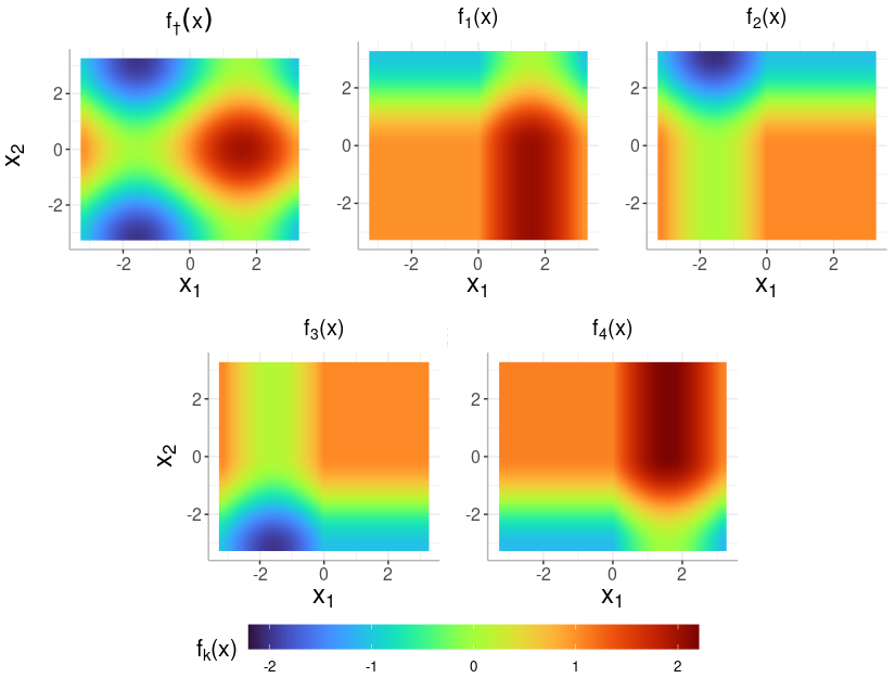
Figure 6: The true underlying process, $f_{\dagger}(\boldsymbol{x})$, and the output from the $K=4$ simulators $f_{1}(\boldsymbol{x}),\ldots,f_{4}(\boldsymbol{x})$.

Assume an underlying physical process is given by $f_{\dagger}(\boldsymbol{x})=\sin(x_{1})+\cos(x_{2})$, where $\boldsymbol{x}=(x_{1},x_{2})\in[-\pi,\pi]\times[-\pi,\pi]$, and $Y(\boldsymbol{x})$ is generated as a Gaussian random process with mean $f_{\dagger}(\boldsymbol{x})$ and standard deviation $\sigma=0.05$. Consider $K=4$ different simulators with outputs shown in Figure 6. Compared to $f_{\dagger}(\boldsymbol{x})$, we see each simulator provides a high-fidelity approximation of the system in one corner of the domain, a lower-fidelity approximation in two corners of the domain, and a poor approximation in the last corner of the domain. We generated $n=100$ simulated observations from the true process, $f_{\dagger}(\boldsymbol{x})$, across equally spaced inputs over a regular grid, and then fit an RPBART-BMM model using $m=10$, $k=1$, $\alpha_{1}=2$, $\alpha_{2}=10$, $\alpha=0.95$, and $\beta=1$.

The posterior prediction results are summarized in Figure 7. The left panel displays the mean prediction, which nearly matches the true underlying process shown in Figure 6. The mean residuals (center) suggest the mixed-prediction only struggles in areas where $x_{1}$ or $x_{2}$ are close to $0$, the region where each simulator begins to degrade. The width of the credible intervals (right) displays a similar pattern with low uncertainty in each corner and larger uncertainty in the middle of the domain.

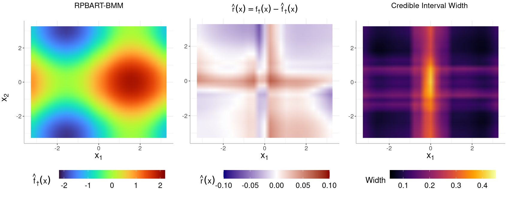
Figure 7: (Left) The mean prediction of the underlying system from the RPBART-BMM model by mixing the outputs of $K=4$ simulators. (Center) The residuals between the underlying process $f_{\dagger}(\boldsymbol{x})$ and the mean prediction $\hat{f}_{\dagger}(\boldsymbol{x})$. (Right) The interval width of the pointwise $95\%$ Credible Intervals from the RPBART-BMM model.

The posterior mean of the weight functions are shown in Figure 8. Each individual weight suggests the corresponding simulator receives relatively high weight in one corner, moderate weight in two corners, and relatively low or negative weight in the last corner. For example consider the first simulator and correspond mean weight $\hat{w}_{1}(\boldsymbol{x})$. We see the corner with higher weight (yellow) corresponds to the region where that particular simulator is a high-fidelity approximation of the system. The two corners (top left and bottom right) where the simulator receives lower but non-negligible weight (pink and purple) generally corresponds to the region where the model is less accurate but still informative for the underlying process. The region where the simulator receives weight near 0 or negative (blue and black) generally corresponds to the area where the model does not follow the patterns of the underlying process.

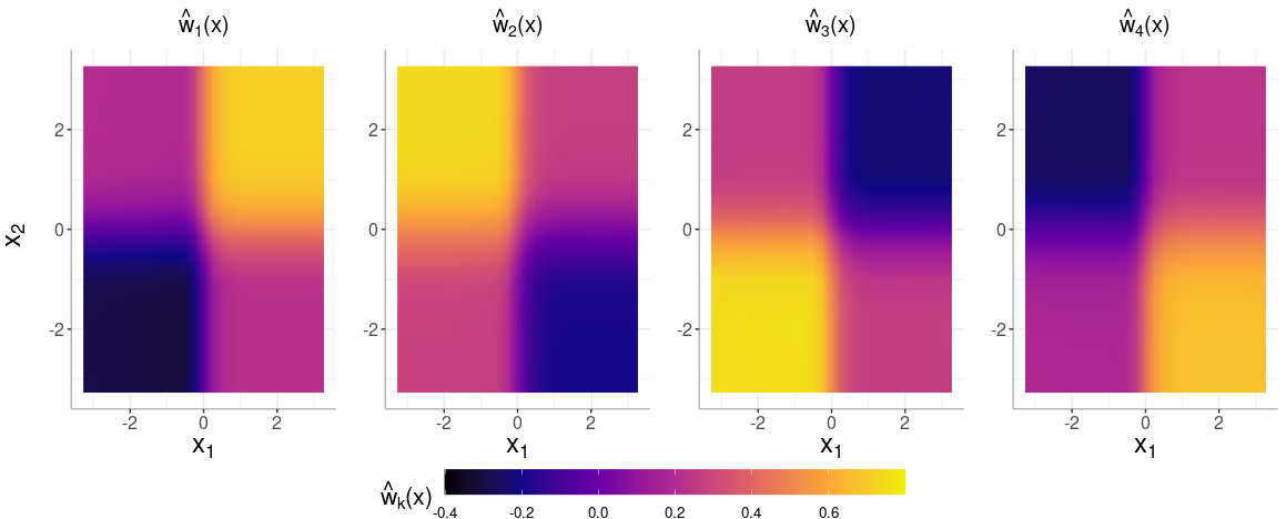
Figure 8: The posterior mean weight functions from the RPBART-BMM model.

Overall, the RPBART-BMM model is able to identify regions where a given simulator is a high or low fidelity approximation of the system. The mean prediction and weight functions are estimated as continuous functions, which improves upon the initial work of Yannotty et al. (2024).

5.2 Application to Climate Data Integration

In this application, we mix multiple GCMs which model the monthly average two-meter surface temperature (T2M) across the world for April, August, and December 2014. These three time periods are chosen to capture how the GCM performance varies across different months. We combine the output of eight different simulators, each with varying fidelity across the input space and spatial resolution.

We compare the RPBART-BMM approach to Feature-Weighted Linear Stacking (FWLS) (Sill et al., 2009) and Neural Network Stacking (NNS) (Coscrato et al., 2020). The latter two approaches are both mean mixing methods where FWLS models the weights using a linear model and NNS defines the weights using a Neural Network. We allow all three methods to model the weights as functions of latitude, longitude, elevation, and month. Each mixing method is trained using 45,000 observations, where 15,000 are taken from each of the three time periods. The predictions for April, August, and December 2014 are generated over a grid of 259,200 latitude and longitude pairs for each time period.

5.2.1 Results

Model	April 2014	August 2014	December 2014
RPBART-BMM	0.827	0.864	0.882
NNS	0.993	1.032	1.088
FWLS	2.393	2.345	2.142
Access	3.675	3.813	4.802
BCC	4.229	4.320	4.340
MIROC	5.529	5.590	6.979
CMCC	4.454	4.272	6.369
CESM2	3.230	3.681	3.419
CNRM	3.289	3.053	3.580
Can-ESM5	3.665	3.977	3.759
KIOST	3.763	4.645	3.639

Table 1: The root mean square error for each mixing approach (BART-BMM, NNS, and FWLS) and GCMs (remaining rows) stratified by month. Each RMSE is computed by evaluating the output of the mixed-prediction or a given GCM over a dense grid of 259,200 inputs and comparing to the observed ERA5 data. Smallest RMSEs for each month are denoted in bold.

We downloaded the GCM data from the Coupled Model Intercomparison Project (CMIP6) (Eyring et al., 2016), a data product which includes outputs from a wide range of simulators used to study various climate features. Each GCM may be constructed on a different set of external forcing or socioeconomic factors, hence the fidelity of each climate model is likely different across the globe. Regardless of these factors, each GCM outputs the T2M on a longitude and latitude grid although the grid resolutions can be different. We denote the output from each GCM at a given input $\boldsymbol{x}$ as $f_{l}(\boldsymbol{x})$ where $l=1,\ldots,K$.

In climate applications, reanalysis data is often used for observational data. We obtain the European Centre for Medium-Range Forecasts reanalysis (ERA5) data, which combines observed surface temperatures with results from a weather forecasting model to produce measurements of T2M across a dense grid of $0.25^{\circ}$ longitude by $0.25^{\circ}$ latitude. We denote the $i\text{th}$ reanalysis data point as $Y(\boldsymbol{x}_{i})$ where $\boldsymbol{x}_{i}$ denotes the $i\text{th}$ latitude, longitude, elevation, and month for $i=1,\ldots,45000$. The ERA5 data and elevation data was downloaded from the Copernicus Climate Data Store.

A common assumption in model mixing is that the simulators are evaluated across the same grid of inputs as the observed response data. To map the data onto the same grid, we apply the bilinear interpolation to obtain an inexpensive emulator, $\hat{f}_{1}(\boldsymbol{x}),\ldots,\hat{f}_{K}(\boldsymbol{x}),$ for each GCM (The Climate Data Guide: Regridding Overview., 2014).

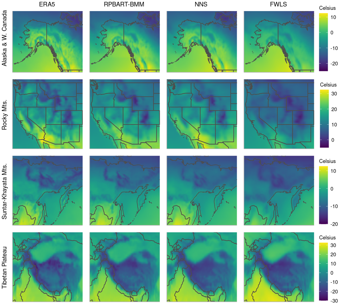
Figure 9: The ERA5 data (first column) vs the mean predictions from RPBART-BMM (second column), NNS (third column), or FWLS (fourth column). Each row highlights difference regions of the world in April 2014.

Table 1 displays the root mean squared errors for each of the three time periods. We see each of the three mean mixing approaches (RPBART-BMM, NNS, FWLS) outperform the individual simulators (rows 4-11), with the RPBART-BMM model performing the best across each month. Figure 9 displays the ERA5 data (left) and the mean predictions from the three approaches across Alaska and Western Canada, the Rocky Mountains, the Suntar-Khayata Mountain Region, and the Tibetan Plateau in April 2014. In general, we see RPBART-BMM and NNS result in very similar high-fidelity predictions that capture the granular features in the data. Some of the granularity is lost in FWLS due to the less flexible form of the weight functions defined by a linear basis. Only subtle differences exist between RPBART-BMM and NNS. It appears RPBART-BMM is able to better leverage elevation and preserve the fine details in the data, as seen in the predictions in the Suntar-Khayata Mountains and the Tibetan Plateau.

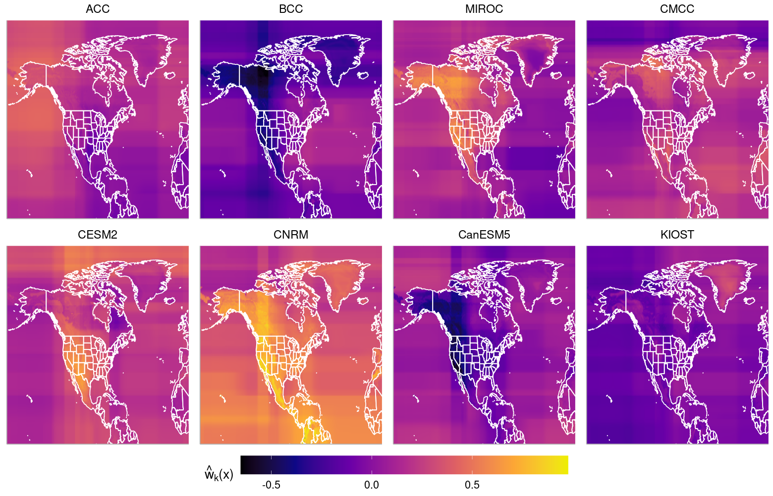
Figure 10: The posterior mean of the RPBART-based weight functions for each of the eight simulators across the northwestern hemisphere in April 2014.

In addition to the improved mean prediction, we are also interested in identifying the subregions where each simulator is favored in the ensemble. In most cases, we have observed weight values closer to $1$ typically indicates more accurate GCMs, while weights near $0$ typically indicate less accurate GCMs. Figure 10 displays the posterior mean weight functions for the eight simulators in the Northwestern hemisphere in April 2014. The posterior mean weights in Figure 10 suggest CNRM, CESM2, and MIROC are more active in the mixed-prediction across the western part of the U.S. and Canada, as these three GCMs receive higher weight relative to the other GCMs. In the same region, BCC and CanESM5 receive negative weights, which are possibly due to multicollinearity and can be investigated using posterior weight projections as described in Section 4.3.

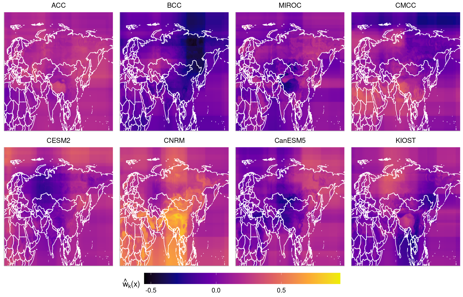
Figure 11: The posterior mean of the RPBART-based weight functions for each of the eight simulators across the northeastern hemisphere in April 2014.

Figure 11 displays the posterior mean weight functions for the GCMs in the Northeastern hemisphere for April 2014. Again we can identify the subregions where each of the GCMs are more active in the mixed-prediction and receive higher weight. Additionally, we can identify the effect of elevation across the eight weights. For example, we can easily identify the oval shape of the Tibetan Plateau in South Asia across the various weight functions. Additionally, we can identify the outline of Suntar-Khayata mountain regions in Northeastern Asia based on the weights attributed to CNRM and CanESM5.

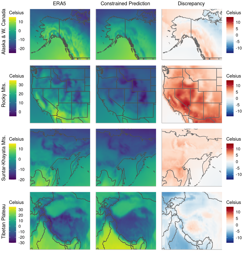
Figure 12: The ERA5 data (left) vs. the simplex constrained mixture of simulators (center) and the resulting additive discrepancy (right) across four subregions (rows) in April 2014.

To better identify a subset of GCMs that are active in a specific region, we consider projecting the samples of the posterior weight functions onto the simplex using a penalized $L_{2}$ projection (the sparsegen-linear projection) (Laha et al., 2018). This imposes a sum-to-one and non-negativity constraint on $\boldsymbol{u}(\boldsymbol{x})$. For this example, $T=0.137$, which is chosen by minimizing the sum of squared discrepancies, $\sum_{i=1}^{N_{v}}\big{(}\delta(\boldsymbol{x}^{v}_{i})\big{)}^{2}$, at $N_{v}=5000$ validation points.

The posterior mean predictions from the constrained mixture of GCMs and the posterior mean discrepancy are shown in Figure 12. Overall, the constrained mixed-prediction recovers the major features of the underlying temperature patterns, however some fine details are lost due to the simplex constraint. This, at times, can be indicative of response features that are not accounted for by any of the GCMs in the model set. Typically, we loose some of the granularity in the areas with significant elevation changes, such as the Rocky Mountains (second row). Essentially, the constrained weights lose flexibility and are less able to properly account for the discrepancy present in the GCMs, as expected. The remaining variability that is unaccounted for by the constrained mixed-prediction is then attributed to the additive discrepancy.

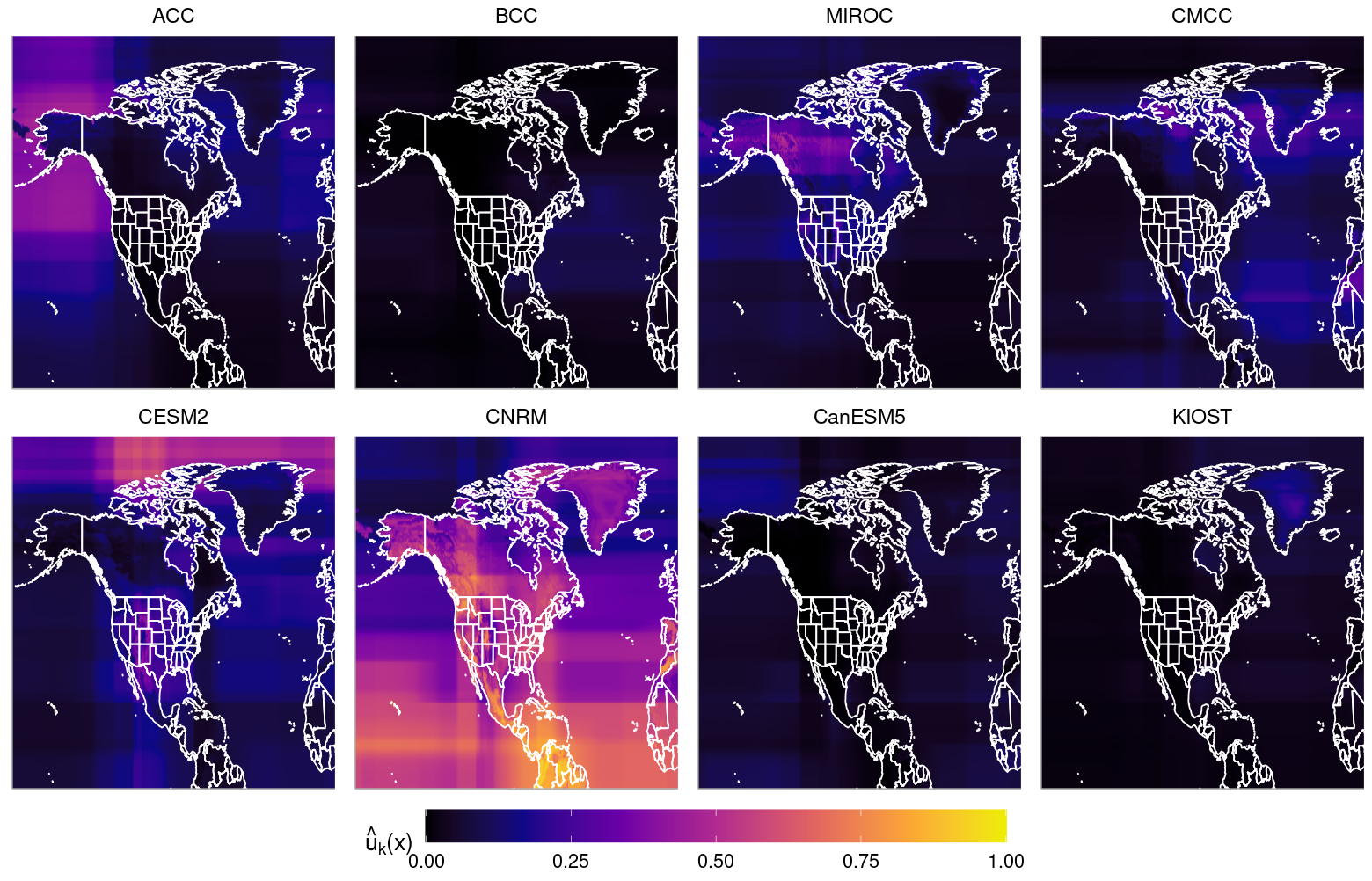
Figure 13: The posterior mean of the constrained RPBART-based weight functions for each of the eight simulators across the northwestern hemisphere in April 2014.

Figure 13 displays the projected weight functions for April 2014. Similar conclusions can be made as in the unconstrained weights from Figure 10, however in the constrained model, we can clearly isolate the GCMs that contribute to the prediction in Figure 12. For example, we see CNRM, CESM2, and MIROC receive relatively high weight in the western part of the United States and Canada. Coupled with the discrepancy in Figure 12, we see that these three GCMs are sufficient for recovering the system in Alaska and Western Canada (low additive discrepancy), but are insufficient for recovering the system in the Rocky Mountains (higher additive discrepancy). Figure 14 displays the posterior mean of the constrained weights in the northeastern hemisphere for April 2014. Similar conclusions can be made as in the northwestern hemisphere.

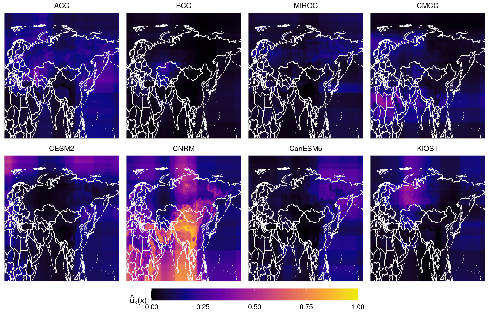
Figure 14: The posterior mean of the constrained RPBART-based weight functions for each of the eight simulators across the northeastern hemisphere in April 2014.

Finally, we can connect the unconstrained and constrained models in terms of how each identifies model discrepancy. In the unconstrained model, the posterior sum of the weight functions, $w_{sum}(\boldsymbol{x})=\sum_{l=1}^{K}w_{l}(\boldsymbol{x})$, is one metric that can be used to help identify model discrepancy. In our applications, we have observed that the posterior distribution of $w_{sum}(\boldsymbol{x})$ deviates away from $1$ in areas where the GCMs do not accurately model the underlying system. This phenomenon has also been observed in earlier work with constant weights (Breiman, 1996; Le and Clarke, 2017). The top panel of Figure 15 displays the posterior mean of $w_{sum}(\boldsymbol{x})$ over selected regions in April 2014. The bottom row of Figure 15 displays the posterior mean of $\delta(\boldsymbol{x})$ from the constrained model in April 2014. Subregions where $w_{sum}(\boldsymbol{x})$ deviates away from $1$ (purple or green) align well with the areas where $\delta(\boldsymbol{x})$ deviates away from $0$ (orange or blue). Thus, the post-processing approach used to estimate $\delta(\boldsymbol{x})$ preserves the information in the posterior of $w_{sum}(\boldsymbol{x})$.

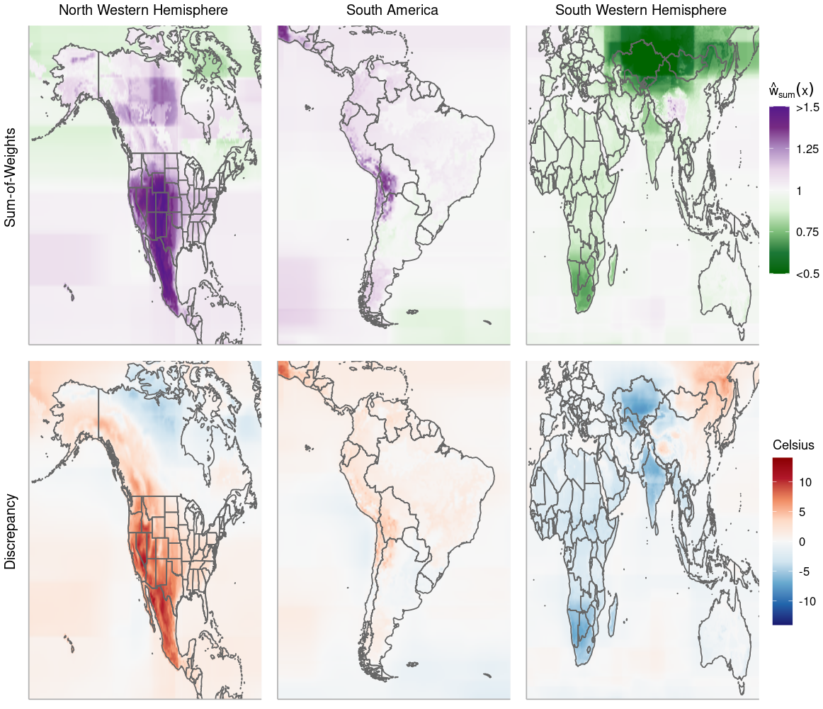
Figure 15: The sum-of-weights from the unconstrained RPBART model (top) and the additive discrepancy from the constrained weight model (bottom). Each column corresponds to a different region in April 2014.

6 Discussion

This research proposes a random path model as a novel approach to introduce continuity into the sum-of-trees model. We then extend the original mean mixing framework presented by Yannotty et al. (2024) to combine the outputs from a general collection of GCMs while also modeling the weight functions as continuous functions. This methodology has been successfully applied to GCMs, which model the monthly average surface temperate.

This model mixing approach depends on two sources of information, namely the observational data and the output from the GCMs. Our method explicitly assumes one can evaluate each GCM, or an emulator for the GCM, at the $n$ inputs associated with the observational data. In this case, each emulator is constructed using bilinear interpolation with respect to the latitude and longitude grid associated with the temperature output. This results in a simple, yet lower resolution emulator for each GCM. Since the emulators maintain a lower resolution, the weight functions in the RPBART-BMM model are left to account for the granularity in the observed data. In other words, when the emulators are lower resolution, the weight functions must be more complex. In terms of BART, the required complexity corresponds to deep trees, less smoothing, and larger $m$.

Alternatively, one could replace the bilinear interpolation approach with a more complex emulator, such as another RPBART model, neural networks, or Gaussian processes (Watson-Parris, 2021; Kasim et al., 2021). More complex emulators could depend on more features other than longitude and latitude and thus result in higher fidelity interpolations of the GCM output. Higher resolution emulators would likely explain more granularity in the data and thus result in less complex weight functions (this implies shallower trees, more smoothing, and smaller $m$).

Existing climate ensembles tend to focus on the temporal distribution of the simulator output and combine the GCM output in a pointwise manner for each latitude and longitude pair (Vrac et al., 2024; Harris et al., 2023). Though a temporal component can be considered as an input to the weight functions, this work predominantly focuses on learning the spatial distribution of the weights to help identify subregions where each simulator is more or less influential. Future work will further explore other ways to incorporate the temporal distribution of the GCMs, which could allow for more appropriate long term model-mixed predictions of future temperature.

7 Acknowledgements

The work of JCY was supported in part by the National Science Foundation under Agreement OAC-2004601. The work of MTP was supported in part by the National Science Foundation under Agreements DMS-1916231, DMS-1564395, OAC-2004601. The work of TJS was supported in part by the National Science Foundation under Agreement DMS-1564395 (The Ohio State University). The work of BL was supported in part by the National Science Foundation under Agreement DMS-2124576.

8 Supplement

8.1 The Conditional Covariance Model

We can better understand the parameters in the RPBART model by studying their effects on the covariance of the response for two inputs, $\boldsymbol{x}$ and $\boldsymbol{x}^{\prime}$. Conditional on the set of trees, $T_{1},\ldots,T_{m}$, bandwidth parameters $\gamma_{1},\ldots,\gamma_{m}$, and error variance $\sigma^{2}$, the prior covariance between $Y(\boldsymbol{x})$ and $Y(\boldsymbol{x}^{\prime})$ is given by Theorem 8.1.

Theorem 8.1 (Conditional Covariance).

Assume the $m$ sets of terminal node parameters, $M_{1},\ldots,M_{m}$, and random path assignments, $Z_{1},\ldots,Z_{m}$ are mutually independent conditional on the set of trees and bandwidth parameters. Further assume that the random path assignments for an observation $\boldsymbol{x}$ are conditionally independent of those for another input $\boldsymbol{x}^{\prime}$. Then, conditional on the set of trees, $T_{1},\ldots,T_{m}$, bandwidth parameters $\gamma_{1},\ldots,\gamma_{m}$, and error variance $\sigma^{2}$ the prior covariance between $Y(\boldsymbol{x})$ and $Y(\boldsymbol{x}^{\prime})$ when $\boldsymbol{x}\neq\boldsymbol{x}^{\prime}$ is given by

$$\text{Cov}\big{(}Y(\boldsymbol{x}),\;Y(\boldsymbol{x}^{\prime})\mid\Theta\big{)}=m\tau^{2}\sum_{j=1}^{m}\frac{1}{m}\sum_{b=1}^{B_{j}}\phi_{bj}(\boldsymbol{x};T_{j},\gamma_{j})\phi_{bj}(\boldsymbol{x}^{\prime};T_{j},\gamma_{j}),$$ (18)

where $\Theta=\big{\{}\{T_{j},\gamma_{j}\}_{j=1}^{m},\sigma^{2}\big{\}}$. The conditional variance is given by

$$\text{Var}\big{(}Y(\boldsymbol{x})\mid\Theta\big{)}=m\tau^{2}+\sigma^{2}.$$ (19)

Proof.

Fix the set of trees, bandwidth parameters, and $\sigma^{2}$ and let $\Theta=\Big{\{}\{T_{j},\gamma_{j}\}_{j=1}^{m},\sigma^{2}\Big{\}}$. By definition, the conditional covariance between $Y(\boldsymbol{x})$ and $Y(\boldsymbol{x}^{\prime})$ is given by

$$\text{Cov}\Big{(}Y(\boldsymbol{x}),\;Y(\boldsymbol{x}^{\prime})\mid\Theta\Big{)} =\text{Cov}\Big{(}\sum_{j=1}^{m}g(\boldsymbol{x};T_{j},M_{j},Z_{j})+\epsilon(\boldsymbol{x}),\;\sum_{k=1}^{m}g(\boldsymbol{x}^{\prime};T_{k},M_{k},Z_{k})+\epsilon(\boldsymbol{x}^{\prime})\mid\Theta\Big{)}$$

$$=\sum_{j=1}^{m}\sum_{k=1}^{m}\text{Cov}\big{(}g(\boldsymbol{x};T_{j},M_{j},Z_{j}),\;g(\boldsymbol{x}^{\prime};T_{k},M_{k},Z_{k})\mid\Theta\big{)}.$$

where $g(\boldsymbol{x};T_{j},M_{j},Z_{j})=\sum_{b=1}^{B_{j}}\mu_{bj}z_{bj}(\boldsymbol{x})$ and $\boldsymbol{x}\neq\boldsymbol{x}^{\prime}$. Due to the conditional independence assumption across the $m$ trees and associated parameters, the covariance simplifies as

$$\text{Cov}\Big{(}Y(\boldsymbol{x}),\;Y(\boldsymbol{x}^{\prime})\mid\Theta\Big{)} =\sum_{j=1}^{m}\text{Cov}\Big{(}g(\boldsymbol{x};T_{j},M_{j},Z_{j}),\;g(\boldsymbol{x}^{\prime};T_{j},M_{j},Z_{j})\mid\Theta\Big{)},$$ (20)

since $\text{Cov}\big{(}g(\boldsymbol{x};T_{j},M_{j},Z_{j}),\;g(\boldsymbol{x}^{\prime};T_{k},M_{k},Z_{k})\mid\Theta\big{)}=0$ when $j\neq k$. Finally, we can consider the covariance function within the $j\text{th}$ tree, which simplifies as follows

$$\text{Cov}\Big{(}g(\boldsymbol{x};T_{j},M_{j},Z_{j}),\;g(\boldsymbol{x}^{\prime};T_{j},M_{j},Z_{j})\mid\Theta\Big{)} =\text{Cov}\Big{(}\sum_{b=1}^{B_{j}}\mu_{bj}z_{bj}(\boldsymbol{x}),\;\sum_{d=1}^{B_{j}}\mu_{dj}z_{dj}(\boldsymbol{x}^{\prime})\mid\Theta\Big{)}$$

$$=\sum_{b=1}^{B_{j}}\sum_{d=1}^{B_{j}}\text{Cov}\Big{(}\mu_{bj}z_{bj}(\boldsymbol{x}),\;\mu_{dj}z_{dj}(\boldsymbol{x}^{\prime})\mid\Theta\Big{)}.$$

Once again, conditional independence between the terminal node parameters and random path assignments implies $\text{Cov}\big{(}\mu_{bj}z_{bj}(\boldsymbol{x}),\;\mu_{dj}z_{dj}(\boldsymbol{x}^{\prime})\big{)}=0$ when $b\neq d$. However, when $b=d$ the covariance within the $j\text{th}$ tree is defined by

$$\sum_{b=1}^{B_{j}}\text{Cov}\big{(}\mu_{bj}z_{bj}(\boldsymbol{x}),\;\mu_{bj}z_{bj}(\boldsymbol{x}^{\prime})\mid\Theta\big{)} =\sum_{b=1}^{B_{j}}E\big{[}\mu_{bj}^{2}z_{bj}(\boldsymbol{x})z_{bj}(\boldsymbol{x}^{\prime})\mid\Theta\big{]}$$

$$\qquad-E\big{[}\mu_{bj}z_{bj}(\boldsymbol{x})\mid\Theta\big{]}E\big{[}\mu_{bj}z_{bj}(\boldsymbol{x}^{\prime})\mid\Theta\big{]}$$

$$=\tau^{2}\sum_{b=1}^{B_{j}}\phi_{bj}(\boldsymbol{x};T_{j},\gamma_{j})\;\phi_{bj}(\boldsymbol{x}^{\prime};T_{j},\gamma_{j}),$$

where $E\big{[}\mu_{bj}z_{bj}(\boldsymbol{x})\big{]}=0$ because each terminal node parameter has mean zero and we assume conditional independence between each $\mu_{bj}$ and $z_{bj}(\boldsymbol{x})$. Returning to (20), the covariance between $Y(\boldsymbol{x})$ and $Y(\boldsymbol{x}^{\prime})$ when $\boldsymbol{x}\neq\boldsymbol{x}^{\prime}$ is then defined as

$$\text{Cov}\big{(}Y(\boldsymbol{x}),\;Y(\boldsymbol{x}^{\prime})\mid\Theta\big{)}=m\tau^{2}\sum_{j=1}^{m}\frac{1}{m}\sum_{b=1}^{B_{j}}\phi_{bj}(\boldsymbol{x};T_{j},\gamma_{j})\phi_{bj}(\boldsymbol{x}^{\prime};T_{j},\gamma_{j}).$$

An expression for the conditional variance of $Y(\boldsymbol{x})$ is also given by

$$\text{Var}\big{(}Y(\boldsymbol{x})\mid\Theta\big{)} =\text{Var}\big{(}\sum_{j=1}^{m}g(\boldsymbol{x};T_{j},M_{j},Z_{j})+\epsilon(\boldsymbol{x})\mid\Theta\big{)}$$

$$=\sum_{j=1}^{m}\text{Var}\big{(}g(\boldsymbol{x};T_{j},M_{j},Z_{j})\mid\Theta\big{)}+\text{Var}\big{(}\epsilon(\boldsymbol{x})\mid\Theta\big{)}.$$ (21)

Due to the conditional independence between parameters across trees, we can once again focus on the variance within each tree separately. The conditional variance for the output of $T_{j}$ is

$$\text{Var}\Big{(}g(\boldsymbol{x};T_{j},M_{j},Z_{j})\mid\Theta\Big{)} =\text{Var}\Big{(}\sum_{b=1}^{B_{j}}\mu_{bj}z_{bj}(\boldsymbol{x})\mid\Theta\Big{)}$$

$$=E\Big{[}\Big{(}\sum_{b=1}^{B_{j}}\mu_{bj}z_{bj}(\boldsymbol{x})\Big{)}^{2}\mid\Theta\Big{]}-E\Big{[}\sum_{b=1}^{B_{j}}\mu_{bj}z_{bj}(\boldsymbol{x})\mid\Theta\Big{]}^{2}$$

$$=\sum_{b=1}^{B_{j}}\sum_{d=1}^{B_{j}}E\Big{[}\mu_{bj}\mu_{dj}z_{bj}(\boldsymbol{x})z_{dj}(\boldsymbol{x})\mid\Theta\Big{]}.$$

By assumption, $z_{bj}(\boldsymbol{x})\in\{0,1\}$ and $\sum_{b=1}^{B_{j}}z_{bj}(\boldsymbol{x})=1$. Thus, if $b\neq d$, then $z_{bj}(\boldsymbol{x})z_{dj}(\boldsymbol{x})=0$ with probability 1. The conditional variance then simplifies as

$$\text{Var}\big{(}g(\boldsymbol{x};T_{j},M_{j},Z_{j})\mid\Theta\big{)} =\sum_{b=1}^{B_{j}}E\big{[}\mu_{bj}^{2}z^{2}_{bj}(\boldsymbol{x})\mid\Theta\big{]}$$

$$=\sum_{b=1}^{B_{j}}E\big{[}\mu_{bj}^{2}z_{bj}(\boldsymbol{x})\mid\Theta\big{]}$$

$$=\sum_{b=1}^{B_{j}}\tau^{2}\phi_{bj}(\boldsymbol{x};T_{j},\gamma_{j})$$

$$=\tau^{2},$$

where $\sum_{b=1}^{B_{j}}\phi_{bj}(\boldsymbol{x};T_{j},\gamma_{j})=1$. Thus, the conditional variance of the tree output is simply the variance of the terminal node parameters $\tau^{2}$. The variance of the sum-of-tress is then given by $m\tau^{2}$. These results are the same as in the original BART model. Returning to (21), the conditional variance of $Y(\boldsymbol{x})$ is given by $\text{Var}\big{(}Y(\boldsymbol{x})\mid\Theta\big{)}=m\tau^{2}+\sigma^{2}$. ∎

8.2 Proof of the Semivariogram Formula

Consider the semivariogram of the sum-of-trees model, which depends on the function $\nu(\boldsymbol{x},\boldsymbol{h})$. Due to the constant mean assumption in the random path model, $\nu(\boldsymbol{x},\boldsymbol{h})$ is defined by

$$\nu(\boldsymbol{x},\boldsymbol{h}) =\frac{1}{2}E^{T,M,Z,\gamma}\Big{[}\big{(}Y(\boldsymbol{x}+\boldsymbol{h})-Y(\boldsymbol{x})\big{)}^{2}\mid\sigma^{2}\Big{]}$$

$$=\frac{1}{2}E^{T,\gamma}\Big{[}E^{M,Z}\Big{[}\big{(}Y(\boldsymbol{x}+\boldsymbol{h})-Y(\boldsymbol{x})\big{)}^{2}\mid\Theta\Big{]}\Big{]},$$ (22)

where $E^{T,\gamma}$ denotes the expectation with respect to the set of trees and bandwidth parameters and $E^{M,Z}$ denotes the conditional expectation with respect to the set of terminal nodes and random path assignments. Moving forward, we will let $\Theta=\big{\{}\{T_{j},\gamma_{j}\}_{j=1}^{m},\sigma^{2}\big{\}}$ and treat $\sigma^{2}$ as a fixed value rather than a random variable.

First consider the inner expectation, which will enable us to understand the effect of the priors we assign to each $M_{j}$ and $Z_{j}$ in the model. Due to the constant mean assumption, the inner expectation is equivalently expressed as

$$E^{M,Z}\Big{[}\big{(}Y(\boldsymbol{x}+\boldsymbol{h})-Y(\boldsymbol{x})\big{)}^{2}\mid\Theta\Big{]} =\text{Var}\big{(}Y(\boldsymbol{x}+\boldsymbol{h})\mid\Theta\big{)}$$ (23)

$$\quad\quad+\text{Var}\big{(}Y(\boldsymbol{x})\mid\Theta\big{)}$$

$$\quad\quad-2\;\text{Cov}\big{(}Y(\boldsymbol{x}+\boldsymbol{h}),Y(\boldsymbol{x})\mid\Theta\big{)}.$$

The inner expectation from (23) divided by $2$ will be denoted as $\nu(\boldsymbol{x},\boldsymbol{h};\Theta)$. Thus, we can focus on $\nu(\boldsymbol{x},\boldsymbol{h};\Theta)$, which involves analytically tractable terms, as shown in Theorem 8.1:

$$\nu(\boldsymbol{x},h;\Theta)=\sigma^{2}+m\tau^{2}\Big{(}1-\frac{1}{m}\sum_{j=1}^{m}\sum_{b=1}^{B_{j}}\phi_{bj}(\boldsymbol{x}+\boldsymbol{h};T_{j},\gamma_{j})\phi_{bj}(\boldsymbol{x};T_{j},\gamma_{j})\Big{)}.$$ (24)

The function $\nu(\boldsymbol{x},\boldsymbol{h})$ is obtained by computing the outer expectation in (22), which is with respect to the set of $m$ trees and bandwidth parameters. We can then obtain $\nu(\boldsymbol{x},\boldsymbol{h})$ by marginalizing over the remaining parameters,

$$\nu(\boldsymbol{x},\boldsymbol{h}) =\sigma^{2}+m\tau^{2}E\Big{[}\Big{(}1-\frac{1}{m}\sum_{j=1}^{m}\sum_{b=1}^{B_{j}}\phi_{bj}(\boldsymbol{x}+\boldsymbol{h};T_{j},\gamma_{j})\phi_{bj}(\boldsymbol{x};T_{j},\gamma_{j})\Big{)}\Big{]}$$

$$=\sigma^{2}+m\tau^{2}\Big{(}1-\frac{1}{m}\sum_{j=1}^{m}E\Big{[}\sum_{b=1}^{B_{j}}\phi_{bj}(\boldsymbol{x}+\boldsymbol{h};T_{j},\gamma_{j})\phi_{bj}(\boldsymbol{x};T_{j},\gamma_{j})\Big{]}\Big{)},$$ (25)

where the expectation is with respect to $\Theta$ and $\sigma^{2}$ is treated as a fixed constant.

Since the set of trees and bandwidth parameters are sets of i.i.d. random quantities, the expectation in (25) is the same for each $j=1,\ldots,m$. Finally, we take $\tau=\big{(}y_{max}-y_{min}\big{)}/(2k\sqrt{m})$ which implies $m\tau^{2}$ simplifies as

$$m\tau^{2}=\Big{(}\frac{y_{\text{max}}-y_{\text{min}}}{2k}\Big{)}^{2},$$

where $y_{\text{max}}-y_{\text{min}}$ is the range of the observed data and $k$ is a tuning parameter that controls the flexibility of the sum-of-trees model. Given these two simplifications, $\nu(\boldsymbol{x},\boldsymbol{h})$ for the RPBART is

$$\nu(\boldsymbol{x},\boldsymbol{h}) =\sigma^{2}+\Big{(}\frac{y_{\text{max}}-y_{\text{min}}}{2k}\Big{)}^{2}\Big{(}1-E\Big{[}\sum_{b=1}^{B_{1}}\phi_{b1}(\boldsymbol{x}+\boldsymbol{h};\gamma_{1},T_{1})\phi_{b1}(\boldsymbol{x};\gamma_{1},T_{1})\Big{]}\Big{)}.$$

8.3 The Semivariogram Formula for Model Mixing

Similar to Section 8.2, we first consider the function, $\nu(\boldsymbol{x},\boldsymbol{h};\Theta)$. In model mixing, this is derived by marginalizing over $M_{j}$, $Z_{j}$, and $f_{l}(\boldsymbol{x})$ where $j=1,\ldots,m$ and $l=1,\ldots,K$. For simplicity, assume each $f_{l}(\boldsymbol{x})$ is an independently distributed stochastic process with constant mean $\bar{f}_{l}$ and covariance function $R_{l}(\boldsymbol{x}+\boldsymbol{h},\boldsymbol{x};\boldsymbol{\psi}_{l})$, with hyperparameter vector $\boldsymbol{\psi}_{l}$.

The function $\nu(\boldsymbol{x},\boldsymbol{h};\Theta)$ is defined in Theorem 8.2.

Theorem 8.2.

Assume the set of emulators, $f_{1}(\boldsymbol{x}),\ldots,f_{K}(\boldsymbol{x})$, are mutually independent random processes with constant means $\bar{f}_{l}$ and covariance functions $R_{l}(\boldsymbol{x}+\boldsymbol{h},\boldsymbol{x};\boldsymbol{\psi}_{l})$, $l=1,...,K$. Further assume the emulators are independent of the $K$ weight functions. Then, the function $\nu(\boldsymbol{x},\boldsymbol{h};\Theta)$ for the mean-mixing model is given by

$$\nu(\boldsymbol{x},\boldsymbol{h};\Theta)=\sigma^{2} +\Big{(}m\tau^{2}+\frac{1}{K^{2}}\Big{)}\sum_{l=1}^{K}\nu_{l}^{(f)}(\boldsymbol{x},h;\boldsymbol{\psi}_{l})\;$$

$$\quad+\nu^{(w)}(\boldsymbol{x},h;\Theta)\sum_{l=1}^{K}\Big{(}R_{l}(\boldsymbol{x}+\boldsymbol{h},\boldsymbol{x};\boldsymbol{\psi}_{l})+\bar{f}_{l}^{2}\Big{)}$$

where $\nu^{(f)}_{l}(\boldsymbol{x},h;\boldsymbol{\psi}_{l})=R_{l}(\boldsymbol{x},\boldsymbol{x};\boldsymbol{\psi}_{l})-R_{l}(\boldsymbol{x}+\boldsymbol{h},\boldsymbol{x};\boldsymbol{\psi}_{l})$ is semivariogram component from the $l\text{th}$ emulator, $R(\boldsymbol{x}+\boldsymbol{h},\boldsymbol{x}+\boldsymbol{h};\boldsymbol{\psi}_{l})=R(\boldsymbol{x},\boldsymbol{x};\boldsymbol{\psi}_{l})$, and

$$\nu^{(w)}(\boldsymbol{x},h;\Theta)=m\tau^{2}\Big{(}1-\frac{1}{m}\sum_{j=1}^{m}\sum_{b=1}^{B_{j}}\phi_{bj}(\boldsymbol{x}+\boldsymbol{h};T_{j},\gamma_{j})\phi_{bj}(\boldsymbol{x};T_{j},\gamma_{j})\Big{)}$$

is the semivariogram component from each of the $K$ weight functions.

Proof.

By definition, the function $\nu(\boldsymbol{x},\boldsymbol{h};\Theta)$ is defined by

$$\nu(\boldsymbol{x},\boldsymbol{h};\Theta) =\frac{1}{2}\text{Var}\Big{(}Y(\boldsymbol{x}+\boldsymbol{h})-Y(\boldsymbol{x})\mid\Theta\Big{)}$$

$$=\frac{1}{2}\bigg{(}\text{Var}\Big{(}Y(\boldsymbol{x}+\boldsymbol{h})\mid\Theta\Big{)}+\Big{(}Y(\boldsymbol{x})\mid\Theta\Big{)}\bigg{)}$$

$$\qquad-\text{Cov}\big{(}Y(\boldsymbol{x}+\boldsymbol{h})-Y(\boldsymbol{x})\big{.}$$

The conditional variance simplifies as,

$$\text{Var}\Big{(}Y(\boldsymbol{x})\mid\Theta\Big{)} =\text{Var}\Big{(}\sum_{l=1}^{K}w_{l}(\boldsymbol{x})f_{l}(\boldsymbol{x})+\epsilon(\boldsymbol{x})\mid\Theta\Big{)}$$

$$=\sigma^{2}+\sum_{l=1}^{K}\text{Var}\Big{(}w_{l}(\boldsymbol{x})f_{l}(\boldsymbol{x})\mid\Theta\Big{)},$$

where the $K$ weights and $K$ functions are all mutually independent, conditional on $\Theta$. Each individual variance component then simplifies as

$$\text{Var}\Big{(}w_{l}(\boldsymbol{x})f_{l}(\boldsymbol{x})\mid\Theta\Big{)} =E\Big{[}w_{l}(\boldsymbol{x})^{2}f_{l}(\boldsymbol{x})^{2}\mid\Theta\Big{]}-E\Big{[}w_{l}(\boldsymbol{x})f_{l}(\boldsymbol{x})\mid\Theta\Big{]}^{2}$$

$$=E\big{[}w_{l}(\boldsymbol{x})^{2}\mid\Theta\big{]}E\big{[}f_{l}(\boldsymbol{x})^{2}\big{]}-E\big{[}w_{l}(\boldsymbol{x})\mid\Theta\big{]}^{2}E\big{[}f_{l}(\boldsymbol{x})\big{]}^{2}$$

$$=\Big{(}m\tau^{2}+1/K^{2}\Big{)}\Big{(}R_{l}(\boldsymbol{x},\boldsymbol{x};\boldsymbol{\psi}_{l})+\bar{f}_{l}^{2}\Big{)}-\Big{(}\bar{f}_{l}/K\Big{)}^{2}.$$

Similarly, the conditional variance of $w_{l}(\boldsymbol{x}+\boldsymbol{h})f_{l}(\boldsymbol{x}+\boldsymbol{h})$ is expressed by

$$\text{Var}\Big{(}w_{l}(\boldsymbol{x}+\boldsymbol{h})f_{l}(\boldsymbol{x}+\boldsymbol{h})\mid\Theta\Big{)}=\Big{(}m\tau^{2}+1/K^{2}\Big{)}\Big{(}R_{l}(\boldsymbol{x}+\boldsymbol{h},\boldsymbol{x}+\boldsymbol{h};\boldsymbol{\psi}_{l})+\bar{f}_{l}^{2}\Big{)}-\Big{(}\bar{f}_{l}/K\Big{)}^{2},$$

for $l=1,\ldots,K$.

The conditional covariance can then be computed as

$$\text{Cov}\Big{(}Y(\boldsymbol{x}+\boldsymbol{h}),Y(\boldsymbol{x})\mid\Theta\Big{)} =\text{Cov}\Big{(}\sum_{l=1}^{K}w_{l}(\boldsymbol{x}+\boldsymbol{h})f_{l}(\boldsymbol{x}+\boldsymbol{h}),\;\sum_{t=1}^{K}w_{t}(\boldsymbol{x})f_{t}(\boldsymbol{x})\mid\Theta\Big{)}$$

$$=\sum_{l=1}^{K}\sum_{t=1}^{K}\text{Cov}\Big{(}w_{l}(\boldsymbol{x}+\boldsymbol{h})f_{l}(\boldsymbol{x}+\boldsymbol{h}),\;w_{t}(\boldsymbol{x})f_{t}(\boldsymbol{x})\mid\Theta\Big{)}.$$

Due to conditional independence between the $K$ weight functions and the $K$ emulators, the covariance simplifies as

$$\text{Cov}\Big{(}Y(\boldsymbol{x}+\boldsymbol{h}),Y(\boldsymbol{x})\mid\Theta\Big{)} =\sum_{l=1}^{K}\text{Cov}\Big{(}w_{l}(\boldsymbol{x}+\boldsymbol{h})f_{l}(\boldsymbol{x}+\boldsymbol{h}),\;w_{l}(\boldsymbol{x})f_{l}(\boldsymbol{x})\mid\Theta\Big{)}$$

$$=\sum_{l=1}^{K}E\Big{[}w_{l}(\boldsymbol{x}+\boldsymbol{h})f_{l}(\boldsymbol{x}+\boldsymbol{h})w_{l}(\boldsymbol{x})f_{l}(\boldsymbol{x})\mid\Theta\Big{]}$$

$$\qquad\quad-E\Big{[}w_{l}(\boldsymbol{x}+\boldsymbol{h})f_{l}(\boldsymbol{x}+\boldsymbol{h})\mid\Theta\Big{]}E\Big{[}w_{l}(\boldsymbol{x})f_{l}(\boldsymbol{x})\mid\Theta\Big{]}$$

$$=\sum_{l=1}^{K}E\Big{[}w_{l}(\boldsymbol{x}+\boldsymbol{h})w_{l}(\boldsymbol{x})\mid\Theta\Big{]}E\Big{[}f_{l}(\boldsymbol{x}+\boldsymbol{h})f_{l}(\boldsymbol{x})\Big{]}-\Big{(}\bar{f}_{l}/K\Big{)}^{2}$$

$$=\sum_{l=1}^{K}\big{(}m\tau^{2}\bar{\phi}(\boldsymbol{x},h;\Theta)+1/K^{2}\big{)}\Big{(}R_{l}(\boldsymbol{x}+\boldsymbol{h},\boldsymbol{x};\boldsymbol{\psi}_{l})+\bar{f}_{l}^{2}\Big{)}$$

$$\qquad\quad-\sum_{l=1}^{K}\Big{(}\bar{f}_{l}/K\Big{)}^{2}.$$

where $\bar{\phi}(\boldsymbol{x},h;\Theta)=\frac{1}{m}\sum_{j=1}^{m}\sum_{b=1}^{B_{j}}\phi_{bj}(\boldsymbol{x}+\boldsymbol{h};T_{j},\gamma_{j})\phi_{bj}(\boldsymbol{x};T_{j},\gamma_{j})$. Using the conditional variances and covariance, $\nu(\boldsymbol{x},\boldsymbol{h};\Theta)$ can be expressed as

$$\nu(\boldsymbol{x},\boldsymbol{h};\Theta) =\frac{1}{2}\bigg{(}\sigma^{2}+\sum_{l=1}^{K}\Big{(}R_{l}(\boldsymbol{x}+\boldsymbol{h},\boldsymbol{x}+\boldsymbol{h};\boldsymbol{\psi}_{l})+\bar{f}_{l}^{2}\Big{)}\Big{(}m\tau^{2}+1/K^{2}\Big{)}-\Big{(}\bar{f}_{l}/K\Big{)}^{2}\bigg{)}$$

$$\quad+\frac{1}{2}\bigg{(}\sigma^{2}+\sum_{l=1}^{K}\Big{(}R_{l}(\boldsymbol{x},\boldsymbol{x};\boldsymbol{\psi}_{l})+\bar{f}_{l}^{2}\Big{)}\Big{(}m\tau^{2}+1/K^{2}\Big{)}-\Big{(}\bar{f}_{l}/K\Big{)}^{2}\bigg{)}$$

$$\quad-\Bigg{(}\sum_{l=1}^{K}\big{(}m\tau^{2}\bar{\phi}(\boldsymbol{x},h;\Theta)+1/K^{2}\big{)}\Big{(}R_{l}(\boldsymbol{x}+\boldsymbol{h},\boldsymbol{x};\boldsymbol{\psi}_{l})+\bar{f}_{l}^{2}\Big{)}-\Big{(}\bar{f}_{l}/K\Big{)}^{2}\Bigg{)}$$

$$=\sigma^{2}+\frac{1}{2}\bigg{(}\sum_{l=1}^{K}\Big{(}R_{l}(\boldsymbol{x}+\boldsymbol{h},\boldsymbol{x}+\boldsymbol{h};\boldsymbol{\psi}_{l})\Big{)}\Big{(}m\tau^{2}+1/K^{2}\Big{)}+m\tau^{2}\bar{f}^{2}_{l}\bigg{)}$$

$$\quad+\frac{1}{2}\bigg{(}\sum_{l=1}^{K}\Big{(}R_{l}(\boldsymbol{x},\boldsymbol{x};\boldsymbol{\psi}_{l})\Big{)}\Big{(}m\tau^{2}+1/K^{2}\Big{)}+m\tau^{2}\bar{f}^{2}_{l}\bigg{)}$$

$$\quad-\Bigg{(}\sum_{l=1}^{K}\big{(}m\tau^{2}\bar{\phi}(\boldsymbol{x},h;\Theta)+1/K^{2}\big{)}R_{l}(\boldsymbol{x}+\boldsymbol{h},\boldsymbol{x};\boldsymbol{\psi}_{l})+m\tau^{2}\bar{f}_{l}^{2}\bar{\phi}(\boldsymbol{x},h;\Theta)\Bigg{)}$$

$$=\sigma^{2}+\frac{1}{2}\Big{(}m\tau^{2}+1/K^{2}\Big{)}\bigg{(}\sum_{l=1}^{K}\Big{(}R_{l}(\boldsymbol{x}+\boldsymbol{h},\boldsymbol{x}+\boldsymbol{h};\boldsymbol{\psi}_{l})+R_{l}(\boldsymbol{x},\boldsymbol{x};\boldsymbol{\psi}_{l})\bigg{)}$$

$$\qquad\quad+m\tau^{2}\big{(}1-\bar{\phi}(\boldsymbol{x},h;\Theta)\big{)}\sum_{l=1}^{K}\bar{f}_{l}^{2}$$

$$\qquad\quad-\big{(}m\tau^{2}\bar{\phi}(\boldsymbol{x},h;\Theta)+1/K^{2}\big{)}\sum_{l=1}^{K}R_{l}(\boldsymbol{x}+\boldsymbol{h},\boldsymbol{x};\boldsymbol{\psi}_{l})$$

$$\qquad\quad\pm\Big{(}m\tau^{2}+1/K^{2}\Big{)}\sum_{l=1}^{K}R_{l}(\boldsymbol{x}+\boldsymbol{h},\boldsymbol{x};\boldsymbol{\psi}_{l}),$$

where we can add and subtract $\Big{(}m\tau^{2}+1/K^{2}\Big{)}\sum_{l=1}^{K}R_{l}(\boldsymbol{x}+\boldsymbol{h},\boldsymbol{x};\boldsymbol{\psi}_{l})$ to further simplify the expression. Now define the following functions for each emulator and each weight as

$$\nu^{(f)}_{l}(\boldsymbol{x},\boldsymbol{h};\boldsymbol{\psi}_{l}) =\frac{1}{2}\Big{(}R_{l}(\boldsymbol{x},\boldsymbol{x};\boldsymbol{\psi}_{l})+R_{l}(\boldsymbol{x}+\boldsymbol{h},\boldsymbol{x}+\boldsymbol{h};\boldsymbol{\psi}_{l})-2R_{l}(\boldsymbol{x}+\boldsymbol{h},\boldsymbol{x};\boldsymbol{\psi}_{l})\Big{)}$$ (26)

$$\nu^{(w)}(\boldsymbol{x},\boldsymbol{h};\Theta) =m\tau^{2}\Big{(}1-\bar{\phi}(\boldsymbol{x},h;\Theta)\Big{)}$$ (27)

In typical cases, $R(\boldsymbol{x}+\boldsymbol{h},\boldsymbol{x}+\boldsymbol{h};\boldsymbol{\psi}_{l})=R(\boldsymbol{x},\boldsymbol{x};\boldsymbol{\psi}_{l})$ and thus $\nu^{(f)}_{l}(\boldsymbol{x},h;\boldsymbol{\psi}_{l})$ simplifies further. The terms in the expression can then be rearranged as follows

$$\nu(\boldsymbol{x},\boldsymbol{h};\Theta) =\sigma^{2}+\Big{(}m\tau^{2}+1/K^{2}\Big{)}\sum_{l=1}^{K}\nu^{(f)}_{l}(\boldsymbol{x},\boldsymbol{h};\boldsymbol{\psi}_{l})$$

$$\qquad\quad+\nu^{(w)}(\boldsymbol{x},\boldsymbol{h};\Theta)\bigg{(}\sum_{l=1}^{K}R_{l}(\boldsymbol{x}+\boldsymbol{h},\boldsymbol{x};\boldsymbol{\psi}_{l})+\bar{f}_{l}^{2}\bigg{)}.$$

∎

Theorem 8.2 shows the function $\nu(\boldsymbol{x},\boldsymbol{h};\Theta)$ combines information from the model set and the weight functions. More specifically, we see the expression combines the functions for the individual semivariogram from the $K+1$ different components. Using Theorem 8.2, we can compute the $\nu(\boldsymbol{x},\boldsymbol{h})$ in Definition 3.1 by marginalizing over the set of $m$ trees and bandwidth parameters. The resulting function is given by

$$\nu(\boldsymbol{x},\boldsymbol{h}) =\sigma^{2}+\Big{(}\;\frac{1}{4k^{2}}+\frac{1}{K^{2}}\Big{)}\sum_{l=1}^{K}\nu_{l}^{(f)}(\boldsymbol{x},h;\boldsymbol{\psi}_{l})\;$$

$$\quad+\Big{(}\frac{1}{2k}\Big{)}^{2}\Big{(}1-E\Big{[}\sum_{b=1}^{B_{1}}\phi_{b1}(\boldsymbol{x}+\boldsymbol{h};T_{1},\gamma_{1})\phi_{b1}(\boldsymbol{x};T_{1},\gamma_{1})\Big{]}\Big{)}$$

$$\qquad\quad\times\sum_{l=1}^{K}\Big{(}R_{l}(\boldsymbol{x}+\boldsymbol{h},\boldsymbol{x};\boldsymbol{\psi}_{l})+\bar{f}_{l}^{2}\Big{)}.$$

8.4 Reproducible Examples

8.4.1 Regression Example

Consider the true data generating process

$$Y(\boldsymbol{x}) \sim N\big{(}f_{\dagger}(\boldsymbol{x}),\sigma^{2}\big{)}$$

$$f_{\dagger}(\boldsymbol{x}) =\sin(x_{1})+\cos(x_{2})$$

where $\boldsymbol{x}\in[-\pi,\pi]\times[-\pi,\pi]$. Assume $n=100$ different observations are generated from the true underlying process with $\sigma=0.1$. The inputs $\boldsymbol{x}_{1},\ldots,\boldsymbol{x}_{100}$ are also randomly generated about the two-dimensional input space. We train the random path model using three different settings of the bandwidth prior to demonstrate the smoothing effect of the model. Each of the three models are trained using an ensemble of 20 trees and a value of $k=1$.

Figure 16 displays the mean predictions from the RPBART model along with their associated hyperparameters of $\alpha_{1}$ and $\alpha_{2}$. Based on Figure 16, we see the model with less smoothing (i.e. $\alpha_{1}=2$ and $\alpha_{2}=20$) provides the most accurate predictions across the entire domain. Essentially, this model preserves the localization induced by the tree models but is able to smooth over the hard boundaries. With $\alpha_{1}=2$ and $\alpha_{2}=5$, we see the a similar smooth mean surface, however the prediction is slightly less accurate along the boundaries (particularly when $x_{1}$ is near $-\pi$). We note BART typically struggles along the boundaries when no or minimal data is present, so this occurrence is to be expected. Similar observations can be made as more smoothness is introduced into the model as shown in the bottom right panel of Figure 16, where $\alpha_{1}=10$ and $\alpha_{2}=10$.

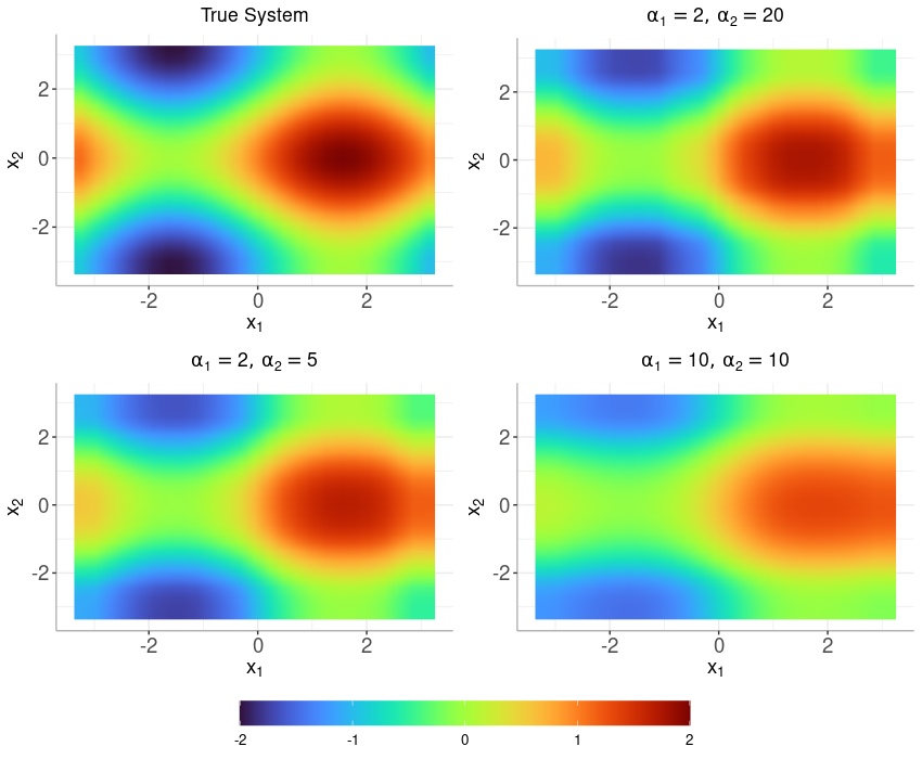
Figure 16: The true system (top left) compared to the the posterior mean of the predictions from the RPBART model using 20 trees and different settings of the bandwidth prior as indicated by the values of $\alpha_{1}$ and $\alpha_{2}$.

These results are to be expected as higher levels of smoothing will naturally result in a less localized prediction. Despite this, RPBART is able to consistently identify the main features of the underlying process, regardless the level of smoothing. In cases with more smoothing, the mean function will identify the general pattern of the data and attribute some of the granularity in the process to the observational error.

8.4.2 Mixing Two GCMs

This section outlines the results from a simplified example which can easily be reproduced on a laptop. Consider mixing the two outputs from CESM2 and CNRM over the Northwestern hemisphere in June 2014. For this example, a 20 tree model is trained using 300 training points. The weight functions are defined only in terms of latitude and longitude. The model is evaluated across a grid of 26,000 points which are evenly spaced over a grid with $0.50^{\circ}\times 0.50^{\circ}$ resolution.

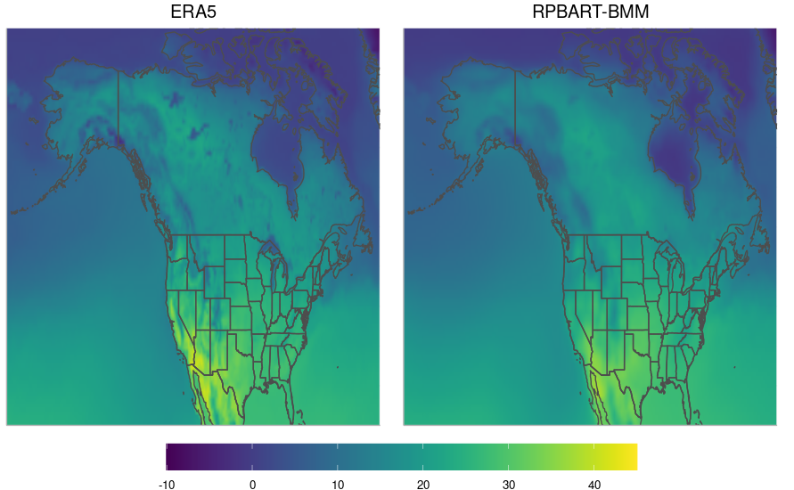
Figure 17: (Left) The observed ERA5 data for June 2014. (Right) The posterior mean prediction from the RPBART-BMM model using 20 trees and 300 training points.

The observed system (left) and posterior mean predictions from RPBART-BMM (right) are shown in Figure 17. We see the mixed-prediction captures the major features within the data, but does not account for some of the granular features in regions of varying elevation. The mixed prediction does not recover these features because only 300 training points are used (compared to the roughly 11,000 points used in Chapter 4 for this region). Additionally, the RPBART-BMM model is only trained using latitude and longitude. Therefore, the model is unable to directly account for any existing discrepancy due to elevation. The resulting weight functions are shown in Figure 18.

Figure 18: The posterior mean of the RPBART-BMM weight functions for GCMs across the northwestern hemisphere in June 2014.

The fidelity of the approximation can be improved by using more training data, including additional simulators, or simply replacing CESM2 and CNRM with higher fidelity models.

References

- (1)
- Breiman (1996) Breiman, L. (1996), “Stacked regressions”, Machine learning 24(1), 49–64.
- Chipman et al. (1998) Chipman, H. A., George, E. I. and McCulloch, R. E. (1998), “Bayesian CART model search”, Journal of the American Statistical Association 93(443), 935–948.
- Chipman et al. (2010) Chipman, H., George, E. and McCulloch, R. (2010), “BART: Bayesian additive regression trees”, The Annals of Applied Statistics 4(1), 266–298.
- Clyde and Iversen (2013) Clyde, M. and Iversen, E. S. (2013), “Bayesian model averaging in the M-open framework”, Bayesian theory and applications pp. 484–498.
- Coscrato et al. (2020) Coscrato, V., de Almeida Inácio, M. H. and Izbicki, R. (2020), “The nn-stacking: Feature weighted linear stacking through neural networks”, Neurocomputing 399, 141–152.
- Cressie (2015) Cressie, N. (2015), Statistics for spatial data, John Wiley & Sons.
- Eyring et al. (2016) Eyring, V., Bony, S., Meehl, G. A., Senior, C. A., Stevens, B., Stouffer, R. J. and Taylor, K. E. (2016), “Overview of the coupled model intercomparison project phase 6 (cmip6) experimental design and organization”, Geoscientific Model Development 9(5), 1937–1958.
- Giorgi and Mearns (2002) Giorgi, F. and Mearns, L. O. (2002), “Calculation of average, uncertainty range, and reliability of regional climate changes from aogcm simulations via the “reliability ensemble averaging”(rea) method”, Journal of climate 15(10), 1141–1158.
- Gringarten and Deutsch (2001) Gringarten, E. and Deutsch, C. V. (2001), “Teacher’s aide variogram interpretation and modeling”, Mathematical Geology 33, 507–534.
- Harris et al. (2023) Harris, T., Li, B. and Sriver, R. (2023), “Multimodel ensemble analysis with neural network gaussian processes”, The Annals of Applied Statistics 17(4), 3403–3425.
- Hastie and Tibshirani (2000) Hastie, T. and Tibshirani, R. (2000), “Bayesian backfitting (with comments and a rejoinder by the authors”, Statistical Science 15(3), 196–223.
- Irsoy et al. (2012) Irsoy, O., Yıldız, O. T. and Alpaydın, E. (2012), Soft decision trees, in “Proceedings of the 21st international conference on pattern recognition (ICPR2012)”, IEEE, pp. 1819–1822.
- Kasim et al. (2021) Kasim, M. F., Watson-Parris, D., Deaconu, L., Oliver, S., Hatfield, P., Froula, D. H., Gregori, G., Jarvis, M., Khatiwala, S., Korenaga, J. et al. (2021), “Building high accuracy emulators for scientific simulations with deep neural architecture search”, Machine Learning: Science and Technology 3(1), 015013.
- Kejzlar et al. (2023) Kejzlar, V., Neufcourt, L. and Nazarewicz, W. (2023), “Local bayesian dirichlet mixing of imperfect models”, Scientific Reports 13(1), 19600.
- Knutti et al. (2017) Knutti, R., Sedláček, J., Sanderson, B. M., Lorenz, R., Fischer, E. M. and Eyring, V. (2017), “A climate model projection weighting scheme accounting for performance and interdependence”, Geophysical Research Letters 44(4), 1909–1918.
- Kong et al. (2020) Kong, W., Krichene, W., Mayoraz, N., Rendle, S. and Zhang, L. (2020), “Rankmax: An adaptive projection alternative to the softmax function”, Advances in Neural Information Processing Systems 33, 633–643.
- Laha et al. (2018) Laha, A., Chemmengath, S. A., Agrawal, P., Khapra, M., Sankaranarayanan, K. and Ramaswamy, H. G. (2018), “On controllable sparse alternatives to softmax”, Advances in neural information processing systems 31.
- Le and Clarke (2017) Le, T. and Clarke, B. (2017), “A Bayes interpretation of stacking for M-complete and M-open settings”, Bayesian Analysis 12(3), 807–829.
- Lin and Dunson (2014) Lin, L. and Dunson, D. B. (2014), “Bayesian monotone regression using gaussian process projection”, Biometrika 101(2), 303–317.
- Linero and Yang (2018) Linero, A. R. and Yang, Y. (2018), “Bayesian regression tree ensembles that adapt to smoothness and sparsity”, Journal of the Royal Statistical Society. Series B (Statistical Methodology) 80(5), 1087–1110.
- Matheron (1963) Matheron, G. (1963), “Principles of geostatistics”, Economic geology 58(8), 1246–1266.
- Phillips et al. (2021) Phillips, D., Furnstahl, R., Heinz, U., Maiti, T., Nazarewicz, W., Nunes, F., Plumlee, M., Pratola, M., Pratt, S., Viens, F. et al. (2021), “Get on the BAND wagon: a Bayesian framework for quantifying model uncertainties in nuclear dynamics”, Journal of Physics G: Nuclear and Particle Physics 48(7), 072001.
- Pratola (2016) Pratola, M. T. (2016), “Efficient Metropolis–Hastings proposal mechanisms for Bayesian regression tree models”, Bayesian analysis 11(3), 885–911.
- Raftery et al. (1997) Raftery, A., Madigan, D. and Hoeting, J. (1997), “Bayesian model averaging for linear regression models”, Journal of the American Statistical Association 92(437), 179–191.
- Sansom et al. (2021) Sansom, P. G., Stephenson, D. B. and Bracegirdle, T. J. (2021), “On constraining projections of future climate using observations and simulations from multiple climate models”, Journal of the American Statistical Association 116(534), 546–557.
- Santner et al. (2018) Santner, T. J., Williams, B. J. and Notz, W. I. (2018), The Design and Analysis of Computer Experiments, 2nd ed., Springer.
- Semposki et al. (2022) Semposki, A. C., Furnstahl, R. J. and Phillips, D. R. (2022), “Interpolating between small- and large- expansions using bayesian model mixing”, Phys. Rev. C 106, 044002.
- Sen et al. (2018) Sen, D., Patra, S. and Dunson, D. (2018), “Constrained inference through posterior projections”, arXiv preprint arXiv:1812.05741 .
- Sill et al. (2009) Sill, J., Takács, G., Mackey, L. and Lin, D. (2009), “Feature-weighted linear stacking”, arXiv preprint arXiv:0911.0460 .
- Tebaldi and Knutti (2007) Tebaldi, C. and Knutti, R. (2007), “The use of the multi-model ensemble in probabilistic climate projections”, Philosophical transactions of the royal society A: mathematical, physical and engineering sciences 365(1857), 2053–2075.
- The Climate Data Guide: Regridding Overview. (2014) The Climate Data Guide: Regridding Overview. (2014), https://climatedataguide.ucar.edu/climate-tools/regridding-overview. Accessed: 2024-03-11.
- Vrac et al. (2024) Vrac, M., Allard, D., Mariéthoz, G., Thao, S. and Schmutz, L. (2024), “Distribution-based pooling for combination and multi-model bias correction of climate simulations”, EGUsphere 2024, 1–41.
- Watson-Parris (2021) Watson-Parris, D. (2021), “Machine learning for weather and climate are worlds apart”, Philosophical Transactions of the Royal Society A 379(2194), 20200098.
- Yannotty et al. (2024) Yannotty, J. C., Santner, T. J., Furnstahl, R. J. and Pratola, M. T. (2024), “Model mixing using bayesian additive regression trees”, Technometrics 66(2), 196–207.
- Yao et al. (2021) Yao, Y., Pirš, G., Vehtari, A. and Gelman, A. (2021), “Bayesian hierarchical stacking: Some models are (somewhere) useful”, Bayesian Analysis 1(1), 1–29.
- Yao et al. (2018) Yao, Y., Vehtari, A., Simpson, D. and Gelman, A. (2018), “Using stacking to average Bayesian predictive distributions”, Bayesian Analysis 13(3), 917–1007.