Domain-specific or Uncertainty-aware models: Does it really make a difference for biomedical text classification?

Abstract

The success of pretrained language models (PLMs) across a spate of use-cases has led to significant investment from the NLP community towards building domain-specific foundational models. On the other hand, in mission critical settings such as biomedical applications, other aspects also factor in—chief of which is a model’s ability to produce reasonable estimates of its own uncertainty. In the present study, we discuss these two desiderata through the lens of how they shape the entropy of a model’s output probability distribution. We find that domain specificity and uncertainty awareness can often be successfully combined, but the exact task at hand weighs in much more strongly.

Domain-specific or Uncertainty-aware models: Does it really make a difference for biomedical text classification?

Aman Sinha^{$\clubsuit$,$\heartsuit$}, Timothee Mickus^$\spadesuit$, Marianne Clausel^$\clubsuit$, Mathieu Constant^$\clubsuit$ and Xavier Coubez^{$\heartsuit$ $\clubsuit$}Université de Lorraine, Nancy, France ^$\spadesuit$University of Helsinki, Helsinki, Finland ^$\heartsuit$Institut de Cancérologie, Strasbourg, France Correspondence: aman.sinha@univ-lorraine.fr

1 Introduction

Deep-learning models are trained with data-driven approaches to maximize prediction accuracy Goodfellow et al. (2016). This entails several well-documented pitfalls, ranging from closed-domain limitations Daume III and Marcu (2006) to social systemic biases McCoy et al. (2019); Schnabel et al. (2016). These limitations compound to a severe deterioration of model performances in out-of-domain (OOD) scenarios Hurd et al. (2013); Shah et al. (2020). This has led to engineering efforts towards developing models tailored to specific domains, ranging from the legal (Paul et al., 2023) to the biomedical (Lee et al., 2020; Singhal et al., 2023) ones.

Domain-specific models, while useful, are rarely considered as a definitive answer. Crucially, in the biomedical domain, experts require more reliability from these models—in particular, insofar as accounting for uncertainty in prediction is concerned. For example, in the case of a risk scoring model used to rank patients for live transplant, uncertainty-awareness becomes critical. The lack of uncertainty-aware models may lead to improper allocation of medical resources Steyerberg et al. (2010). Such concerns exemplify the importance of uncertainty aware models and its critical role in model selection.

The compatibility of domain-specific pretraining and uncertainty modeling appears under-assessed. To illustrate this, one can consider the entropy of output distributions: Domain-specific pretraining will lead to more probability mass assigned to a single (hopefully correct) estimate, leading to a lower entropy; whereas uncertainty-aware designs intend to not neglect valid alternatives—meaning that the probability mass should be spread out, which entails a higher entropy when uncertainty is due.

	Uncertainty-unaware	Uncertainty-aware
General-domain
Domain-specific

Figure 1: Illustration of this study’s setup. We perform a systematic comparison of domain-specificity and uncertainty-awareness in the medical domain.

Dataset		Task Description		Splits				Statistics
				train	val	test		#Class	CIR	avglen	maxlen
US	MedABS	Predict the patient condition described, given a medical abstract		8662	2888	2888		5	3.1445	180.59	597
US	MedNLI	Predict the inference type, given a hypothesis and a premise		11232	1395	1422		3	1	23.83	151
US	SMOKING	Predict the patient smoking status, given a medical discharge record		398	100	104		5	23.75	654.30	2788
FR	PxSLU	Predict the drug prescription intent, given a user speech transcription		1386	198	397		4	98.1538	11.40	48
FR	MedMCQA	Predict the number of answers, given a medical multi-choice question		2171	312	622		5	21.1176	12.90	92
FR	MORFITT	Predict the speciality, given a scientific article abstract		1514	1022	1088		12	15.3529	226.33	1425

Table 1: Datasets description. CIR denotes class imbalance ratio.

In this work, we reflect on how model-specificity and uncertainty-awareness articulate with one another. Figure 1 illustrates the experimental setup we use for our study. In practice, we study the performances of frequentist and Bayesian general and domain-specific models on biomedical text classification tasks across a wide array of metrics, ranging from macro F1 to SCE, with a specific focus on entropy Ruder and Plank (2017); Kuhn et al. (2023). More narrowly, we study the following research questions: RQ1: Are the benefits of uncertainty-awareness and domain-specificity orthogonal? RQ2: Given our benchmarking results, should medical practitioners prioritize domain-specificity or uncertainty-awareness?

2 Related Work

Recently, uncertainty quantification has gained attention from the NLP community Xiao and Wang (2019); Xiao et al. (2022); Hu et al. (2023)—particularly in mission critical settings, such as in the medical domain Hwang et al. (2023); Barandas et al. (2024). In parallel, compared to domain adaptation approaches Wiese et al. (2017) for the medical domain, there is a growing interest in domain-specific language models starting from BioBERT Lee et al. (2020) to the recent MedPalM Singhal et al. (2023). Xiao et al. (2022) presented an elaborate study of uncertainty paradigm for general-domain PLMs. While uncertainty modeling has been applied to biomedical data previously (e.g., Begoli et al., 2019; Abdar et al., 2021), surprisingly little has been done for biomedical textual data. Therefore, our study precisely focuses on the interaction between the two paradigms for medical domain NLP tasks. We address this gap by focusing specifically on predictive entropy Ruder and Plank (2017); Kuhn et al. (2023).

3 Methodology

Datasets.

We conduct experiments on six standard biomedical datasets: three English datasets, viz. MedABS Schopf et al. (2023), MedNLI Romanov and Shivade and SMOKING Uzuner et al. (2008); as well as three French datasets, viz. MORFITT Labrak et al. (2023b), PxSLU Kocabiyikoglu et al. (2022) and MedMCQA Labrak et al. (2023a).

For MEDABS, SMOKING, PxSLU, and MEDMCQA, we do not perform any special preprocessing. For MEDMCQA, we perform Task 2, i.e., predicting the number of possible responses (ranging from 1-5) for the input multi choice question. For MEDNLI, we concatenate the statement and hypothesis using the [SEP] token and use it as an input converting it to a multi-class task. For MORFITT, which is originally a multi-label classification task, we use the first label for each sample to convert it to a multi-class problem. The descriptive statistics of these datasets are listed in Table 1, along with class imbalance ratio (CIR; Yu et al., 2022). See Appendix A.4 for more information.

Models.

We derive classifiers from language-specific PLMs: for English datasets, we use BERT Devlin et al. (2018) and BioBERT Lee et al. (2020); for French, we use CamemBERT Martin et al. (2019) and CamemBERT-bio Touchent et al. (2023). We compare two types of models, frequentist deep learning models (DNN) and Bayesian deep learning models (BNNs). The DNN model comprises of a PLM-based encoder, a Dropout unit along with 1-layer classifier. The BNN models are likewise based on a PLM encoder, along with a Bayesian module applied over the classification layer. We also experimented with MC-dropout models Gal and Ghahramani (2016), DropConnect Mobiny et al. (2021), and variational inference Blundell et al. (2015) models. We focus on the DropConnect architecture which comprises a PLM encoder along a DropConnect dense classification layer. This approach infuses stochasticity into a deterministic model by randomly zeroing out classifier weights with probability $1-p$. This allows us to sample multiple outputs for a given input, thus enabling to aggregate the predictions and to produce estimates of uncertainty.

For simplicity, we note domain-specific models as $+\mathcal{D}$ (and general models $-\mathcal{D}$); uncertainty aware models are referred to as $+\mathcal{U}$ (with frequentist models noted $-\mathcal{U}$). We replicate training across 10 seeds per model and dataset; further implementation details can be found in Section A.2.

Evaluation Setup.

We evaluate classifiers on two aspects: task performance and uncertainty awareness. For text classification, we report Macro-F1 and accuracy. For uncertainty quantification we report Brier score (BS; Brier, 1950), Expected Calibration Error (ECE; Naeini et al., 2015), Static Calibration Error (SCE; Nixon et al., 2019), Negative log likelihood (NLL), coverage (Cov%) and entropy ($H$). See Section A.3 for definitions.

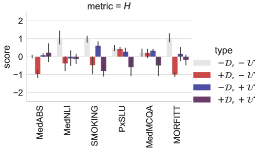
(a) Entropy

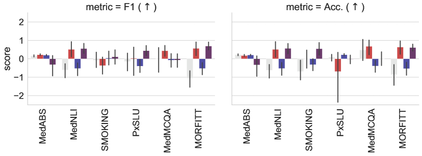
(b) Classification metrics

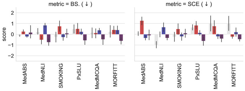
(c) Calibration metrics

Figure 2: Performances for empirically best models (selected metrics), $z$-normalized per dataset. See Table 5 in Appendix B for full non-normalized results.

4 Results

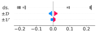
(a) F1

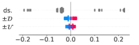
(b) Acc.

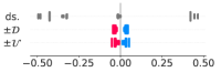
(c) NLL

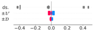
(d) $H$

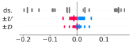
(e) Brier score

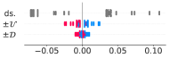
(f) SCE

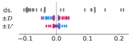
(g) ECE

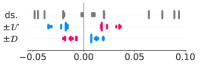
(h) Cov %

Figure 3: SHAP attributions. Variables are ordered by mean absolute SHAPs. In blue, weight assigned when the variable is negative; in red, when it is positive. ‘ds.’ denotes a categorical variable tracking the dataset.

Performance.

All results are listed in Table 5 in Appendix B, we highlight some key metrics in Figure 2. Insofar as classification metrics go, $+\mathcal{D}$ configurations outperform $-\mathcal{D}$ ones. More generally, as all scores are highly dependent on the exact dataset considered, we first de-trend them by $z$-normalizing results on a per-dataset basis to simplify analysis. We find $+\mathcal{D}+\mathcal{U}$ classifiers to be strong contenders, although they are often outperformed—especially by $+\mathcal{D}-\mathcal{U}$ models on classification metrics (Figure 2b) and by $-\mathcal{D}+\mathcal{U}$ models on calibration metrics (Figure 2c). As for entropy, we find both $+\mathcal{D}-\mathcal{U}$ and $+\mathcal{D}+\mathcal{U}$ to lead to lower scores. Trends are consistent across languages.

Relative importance.

To interpret results in Figure 2 more rigorously, we rely on SHAP Lundberg and Lee (2017). SHAP is an algorithm to compute heuristics for Shapley values (Shapley, 1953), viz. a game theoretical additive and fair distribution of a given variable to be explained across predetermined factors of interest. Here, we analyze the scores obtained by individual classifiers on all 8 metrics, and try to attribute their values ($z$-normalized per dataset) to domain specificity ($\pm\mathcal{D}$), uncertainty awareness ($\pm\mathcal{U}$) and the dataset one observation corresponds to (ds.).

Results are displayed in Figure 3; specific points correspond to weights assigned to one of the factors for one of the datapoints, factors are sorted from most to least impactful from top to bottom. We can see that which of domain specificity and uncertainty awareness has the strongest impact depends strictly on the metrics: Cases where $\pm\mathcal{D}$ is assigned on average a greater absolute weight than $\pm\mathcal{U}$ account for exactly half of the metrics we study. Another import trend is that effects tied to $+\mathcal{D}$ are also often attested for $+\mathcal{U}$: if domain specificity is useful, then uncertainty awareness is as well. Lastly, weights assigned to both $\pm\mathcal{D}$ and $\pm\mathcal{U}$ are considerably smaller than those assigned to datasets, showcasing that these trends are often overpowered by the specifics of the task at hand.

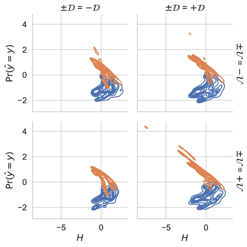
Figure 4: Entropy vs. probability mass assigned to the target ($z$-normalized per classifier). Orange: correct predictions; Blue: incorrect.

Entropy.

A desideratum we laid out above is to have large entropy scores when the model is incorrect. Focusing on entropy, we display how it compares to the probability mass assigned to the target in Figure 4. In detail, we retrieve all predictions for every datapoint across all classifiers and then $z$-normalize entropy scores and probability assigned the target class. We can see that incorrect predictions do result in more spread out entropy scores. Moreover, we can notice some tentative differences between the four types of classifiers of our study: Correct predictions from $+\mathcal{D}+\mathcal{U}$ models seem to lead to an especially tight correlation between entropy and probability mass.

	effect size $f$				Spearman’s $\rho$
	$-\mathcal{D}~{}-\mathcal{U}$	$+\mathcal{D}~{}-\mathcal{U}$	$-\mathcal{D}~{}+\mathcal{U}$	$+\mathcal{D}~{}+\mathcal{U}$	$-\mathcal{D}~{}-\mathcal{U}$	$+\mathcal{D}~{}-\mathcal{U}$	$-\mathcal{D}~{}+\mathcal{U}$	$+\mathcal{D}~{}+\mathcal{U}$
MedABS	$62.4587$	$64.8$64.8	$62.3861$	$67.3204$	$-48.0$-48.0	$-47.9223$	$-44.6260$	$-53.5326$
MedNLI	$73.2472$	$73.2104$	$74.0$74.0	$76.9906$	$-73.1618$	$-77.4$-77.4	$-76.0566$	$-83.2975$
SMOKING	$75.8140$	$71.5580$	$74.1591$	$74.8$74.8	$-56.4635$	$-37.9853$	$-50.0037$	$-56.0$-56.0
PxSLU	$65.4190$	$87.2314$	$65.0581$	$85.8$85.8	$-85.4051$	$-69.0819$	$-87.3$-87.3	$-96.1698$
MedMCQA	$65.5612$	$63.8467$	$66.6$66.6	$68.1908$	$-82.2927$	$-82.2$-82.2	$-60.7625$	$-62.5836$
MORFITT	$65.6$65.6	$66.1075$	$65.0232$	$64.7896$	$-54.6$-54.6	$-55.0504$	$-50.7645$	$-50.9648$

Table 2: Statistical tests on entropy measurements, with best and second best highlighted.

However, establishing whether this difference is significant requires further testing. We therefore measure whether incorrect predictions lead to higher entropy in two ways: (i) using Mann–Whitney U-tests, from which we derive a common language effect size $f$ (as the entropy of incorrect predictions should be higher); and (ii), by computing Spearman correlation coefficients between the entropy and the mass assigned to the target class (as entropy should degrade with correctness). Corresponding results are listed in Table 2: Across most of the datasets we study, the top or second most coherent distributions we observe are for domain-specific and uncertainty-aware models. However, we also observe that actual performances are highly sensitive to the exact classification task at hand.

5 Discussion & Conclusion

We can now answer our initial research questions.

RQ1: Are the benefits of uncertainty-awareness and domain-specificity orthogonal? We have seen in Table 2 that in most cases, using a classifier that was both domain-specific and uncertainty-aware led to the optimal distribution shape, with entropy more gracefully increasing with incorrectness.

RQ2: Should medical practitioners prioritize domain-specificity or uncertainty-awareness? SHAP attributions in Figure 3 strongly suggest that the evaluation metric dictates the strategy to follow. As one would expect, accuracy is better captured with domain-specific models, whereas uncertainty-aware models tend to be better calibrated.

We also found significant evidence throughout our experiments that the exact classification task at hand weighs in much more strongly than the design of the classifier. This extraneous factor necessarily complicates the relationship between domain-specificity and uncertainty-awareness: In a handful of cases in Figure 2, we observe classifiers that are neither uncertainty-aware nor domain specific faring best among all the models we survey—and conversely domain-specific uncertainty-aware classifiers can also rank dead last. This is also related to the often limited quantitative difference between best and worst models, which for instance can be as low as $\pm 2.3\%$ for F1 on MEDABS (cf. Table 5).

Overall, our experiments suggest a very nuanced conclusion. Domain-specificity and uncertainty-awareness do appear to shape classifiers’ distributions and their entropy in distinct but compatible ways, but they have a lesser impact than the task itself. Hence, while we can often combine uncertainty-awareness and domain-specificity, there are no out-of-the-box solutions, and optimal performances require careful application designs.

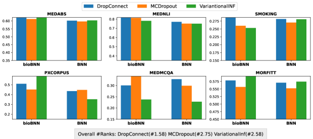
Figure 5: Comparison of various BNN models for different datasets on classification task based on Macro-F1 on validation set.

Appendix A Experimental details

A.1 Supplementary Bayesian models

We include the details for two more Bayesian models: MC-dropout and variational inference. Note that for all the Bayesian models we sample K=3 predictions at inference and use the mean prediction.

MCDropout (MCD)

This model is based on a PLM encoder, similar to the main study models. The difference in this case is that Stochastic Dropout is applied over the classification layer. MCD Gal and Ghahramani (2016) proposes to extend the usage of Dropout but at inference time enabling it to sample a multiple $K$ models, to make $K$ predictions. The final prediction in the case of classification model can denoted as

$$\hat{y}=K^{-1}\sum_{k=1}^{K}f_{i}(x)$$

.

Variational inference (VI)

This model is based on a PLM encoder, similar to the main study models, with variational inference dense layer as the classification layer. We use the Bayes by BackProp Blundell et al. (2015) for the VI Dense layer. It approximates the distribution of each weight with a Gaussian distribution with parameter $\mathcal{N}(\mu,\rho)$. The weights are approximated with Monte Carlo gradient. Finally, the predictions are computed using the predictive posterior distribution, by sampling K weight instances and making one forward pass per set of weights same as MCD.

A.2 Implementation details

We use keras-uncertainty models for implementing our BNN model backbones.

Models		MedABS			MedNLI			SMOKING			PxSLU			MedMCQA			MORFITT
		lr	E		lr	E		lr	E		lr	E		lr	E		lr	E
$-\mathcal{D}$	DNN	1e-5	4		5e-6	12		1e-4	15		5e-6	15		5e-6	14		5e-5	15
$-\mathcal{D}$	DC	5e-6	7		1e-5	11		1e-5	15		5e-6	13		5e-6	15		5e-5	13
$-\mathcal{D}$	MCD	5e-5	5		5e-6	15		5e-5	15		1e-5	14		5e-6	11		5e-5	10
$-\mathcal{D}$	VI	5e-6	7		1e-5	14		5e-6	13		5e-6	14		1e-6	15		5e-5	13
$+\mathcal{D}$	DNN	1e-5	4		1e-5	14		5e-5	15		1e-5	15		1e-5	10		5e-5	15
$+\mathcal{D}$	DC	5e-5	3		1e-5	13		1e-4	13		1e-5	15		5e-6	15		5e-5	13
$+\mathcal{D}$	MCD	5e-5	3		5e-5	12		5e-5	10		1e-5	14		1e-5	15		5e-5	13
$+\mathcal{D}$	VI	1e-5	5		5e-6	13		5e-5	14		1e-5	14		1e-6	15		5e-5	5

Table 3: Best hyparameter for each model configuration and dataset pair. We denote both English and French domain-specific PLMs with $+\mathcal{D}$. The models DC, MCD, VI are from the $+\mathcal{U}$ set.

Hyperparameter Setting

In all cases, we fine-tune the PLM backbone for all the downstream task with a maximum sequence length of 512 and a batch size of 50 sentences. We perform a grid hyper-parameter search for epochs= {3,4,5, ..., 15} and lr= {1e-7, 5e-6, 1e-6, 5e-5, 1e-5, 5e-4, 1e-4}. We replicate training with 3 seeds for each hyperparameter configuration, select the optimal configuration for validation F1, and replicate training with 7 more seeds for these optimal configurations, so as to obtain 10 models per dataset, PLM and architecture. We also select the main BNN model of the study by selecting the system yielding the highest average rank across all six datasets, as displayed in Figure 5.

We train all models with binary cross entropy loss and Adam optimizer with $\epsilon=10^{-8}$ and $\beta=(0.9,0.999)$. For all BNN models, we obtain 3 sets of predictions after training the models to calculate the mean class probabilities. Corresponding optimal hyperparameters are listed in table 3.

A.3 Calibration metrics definition

In what follows, $N$ denotes the number of samples in test set, $C$ denotes the number of classes. Lower score for Brier score, ECE, SCE, NLL and Entropy metrics; and higher score for coverage, are indicative of better uncertainty aware model.

Brier score.

Brier (1950) proposed BS which computes the mean square difference between the true classes and the predicted probabilities.

$$\text{BS}=\frac{1}{N}\sum^{N}_{i=1}\sum^{C}_{c=1}(y^{(i)}_{c}-\hat{y}^{(i)}_{c})^{2}$$

Expected Calibration Error.

Naeini et al. (2015) provides weighted average of the difference between accuracy and confidence across $B$ bins.

$$\text{ECE}=\sum^{B}_{b=1}\frac{n_{b}}{N}|\text{acc}(b)-\text{conf}(b)|$$

where acc$(b)$ and conf$(b)$ are the average accuracy and confidence of predictions in bin $b$, respectively. We set $B=15$ in our experiments.

Static Calibration Error.

Nixon et al. (2019) proposed an extension of ECE to multi-class problems to overcome its limitation of dependence of the number of bins.

$$\text{SCE}=\sum^{C}_{c=1}\sum^{B}_{b=1}\frac{n_{b}}{NC}|\text{acc}(b)-\text{conf}(b)|$$

We set $B=15$ in our experiments.

Negative Log Likelihood.

serves as the primary approach for optimizing neural networks in classification tasks. Interestingly, this loss function can also double as an effective metric for assessing uncertainty.

$$\text{NLL}=-\sum_{i=1}^{N}y_{i}\log(\hat{y}_{i})$$

Coverage Percentage.

The normalized form of number of times the correct class in indeed contain within the prediction set.

Shannon Entropy.

quantifies the expected uncertainty inherent in the possible outcomes of a discrete random variable.

$$H=-\sum_{i=1}^{N}p_{i}\log(p_{i})$$

A.4 Dataset

We provided supplementary details about each dataset we used in Table 4.

Dataset		Sample	Classes	Label Distribution
MedABS Schopf et al. (2023)		{text: "Catheterization of coronary artery bypass graft from the descending aorta. The increasing frequency of reoperation for coronary artery disease has led to the use of a variety of grafts. This report describes the catheter technique for selective opacification of a saphenous vein graft from the descending thoracic aorta to the posterior coronary circulation. ", label: "Cardiovascular diseases" }	{’Neoplasms’, ’Digestive system’, ’Nervous system’, ’Cardiovascular’, ’General pathological’ }	[1925 913 1149 1804 2871]
MedNLI Romanov and Shivade		{text: "No history of blood clots or DVTs, has never had chest pain prior to one week ago. [SEP] Patient has angina", label: "entailment"}	{"entailment", "contradict", "neutral" }	[3744 3744 3744]
SMOKING Uzuner et al. (2008)		{text: "071962960 bh 4236518 417454 12/10/2001 12:00:00 am discharge summary unsigned dis report status : unsigned discharge summary name : sterpsap , ny unit number : 582-96-88 admission date : 12/10/2001 discharge date : 12/19/2001 principal diagnosis : prosthetic aortic valve dysfunction associated diagnoses : aortic valve insufficiency bacterial endocarditis , active principal procedure : urgent re-do aortic valve replacement and correction of left ventricular to aortic discontinuity . ( 12/13/2001 ) other procedures : aortic root aortogram ( 12/12/2001 ) cardiac ultrasound ( 12/13/2001 ) insertion dual chamber pacemaker ( 12/15/2001 ) picc line placement ( 12/18/2001 ) history and reason for hospitalization : mr. sterpsap …", label: "CURRENT SMOKER"}	{’CURRENT SMOKER’, ’NON-SMOKER’, ’PAST SMOKER’, ’SMOKER’, ’UNKNOWN’ }	[ 27 49 24 8 190]
MEDMCQA Labrak et al. (2023a)		{text: "ans la liste suivante, quels sont les antibiotiques utilisables pour traiter une salmonellose chez un adulté?", label: 2}	{1,2,3,4,5}	[595 528 718 296 34]
MORFITT Labrak et al. (2023b)		{text: "La survenue de complications postopératoires représente un cauchemar (bien réel), tant pour le patient que pour son chirurgien. Dès lors, quoi de plus fantasmagorique que d’administrer une « potion magique » au patient avant l’intervention pour éliminer ce risque ? Le but de cet article est de résumer l’état des connaissances actuelles concernant les bénéfices potentiels, liés à l’administration d’immunonutrition aux patients traités pour cancer urologique…..", original_label: [ "Immunologie","Chirurgie",], label: "Immunologie"}	{’Vétérinaire’, ’Étiologie’, ’Psychologie’, ’Chirurgie’, ’Génétique’, ’Physiologie’, ’Pharmacologie’, ’Microbiologie’, ’Immunologie’, ’Chimie’, ’Virologie’, ’Parasitologie’ }	[ 82 261 32 122 40 17 152 39 242 185 104 238]
PxSLU Kocabiyikoglu et al. (2022)		{text: "antacapone 200 milligrammes 2 comprimés le matin 1 comprimé à midi 2 comprimé le soir traitement pour une durée totale de 4 semaines", label: "medical_prescription"}	{"medical_prescription", "negate","replace", "none" }	[1276 15 82 13]

Table 4: Sample data from each Dataset

	Model		Classification			Uncertainty
			Macro-F1($\uparrow$)	Accuracy($\uparrow$)		BS($\downarrow$)	ECE($\downarrow$)	SCE($\downarrow$)	NLL($\downarrow$)	Cov%($\uparrow$)	Entropy($\downarrow$)
MedABS US	$-\mathcal{D}$	DNN	60.3633$\pm$0.003	60.9765$\pm$0.002		0.5535$\pm$0.008	0.1387$\pm$0.016	0.0683$\pm$0.004	1.3261$\pm$0.001	0.8976$\pm$0.013	1.5579$\pm$0.002
	$-\mathcal{D}$	DC	60.9855$\pm$0.004	61.1842$\pm$0.003		0.5518$\pm$0.002	0.1342$\pm$0.007	0.0674$\pm$0.003	1.3192$\pm$0.002	0.9611$\pm$0.003	1.5556$\pm$0.001
	$-\mathcal{D}$	MCD	60.6979$\pm$0.004	60.0993$\pm$0.006		0.5691$\pm$0.015	0.1503$\pm$0.014	0.0688$\pm$0.01	1.3235$\pm$0.008	0.9401$\pm$0.013	1.5542$\pm$0.002
	$-\mathcal{D}$	VI	60.8725$\pm$0.001	61.1611$\pm$0.001		0.5531$\pm$0.006	0.1394$\pm$0.004	0.0695$\pm$0.003	1.3164$\pm$0.003	0.958$\pm$0.001	1.5541$\pm$0.001
	$+\mathcal{D}$	DNN	60.8077$\pm$0.013	61.3343$\pm$0.01		0.5499$\pm$0.014	0.1448$\pm$0.005	0.0695$\pm$0.001	1.3201$\pm$0.014	0.9193$\pm$0.005	1.5561$\pm$0.003
	$+\mathcal{D}$	DC	62.5642$\pm$0.009	62.1018$\pm$0.01		0.5243$\pm$0.015	0.1381$\pm$0.016	0.0624$\pm$0.007	1.2962$\pm$0.007	0.9597$\pm$0.008	1.5523$\pm$0.002
	$+\mathcal{D}$	MCD	62.2038$\pm$0.022	62.1307$\pm$0.022		0.5226$\pm$0.031	0.1238$\pm$0.031	0.0593$\pm$0.015	1.3056$\pm$0.013	0.9666$\pm$0.01	1.5562$\pm$0.002
	$+\mathcal{D}$	VI	63.1893$\pm$0.004	63.1694$\pm$0.003		0.5234$\pm$0.009	0.1464$\pm$0.01	0.0653$\pm$0.003	1.288$\pm$0.006	0.9603$\pm$0.005	1.5491$\pm$0.002
MedNLI US	$-\mathcal{D}$	DNN	73.8951$\pm$0.013	73.8397$\pm$0.015		0.3976$\pm$0.006	0.1278$\pm$0.02	0.0846$\pm$0.012	0.8177$\pm$0.015	0.9119$\pm$0.008	1.0156$\pm$0.008
	$-\mathcal{D}$	DC	74.8161$\pm$0.019	74.8711$\pm$0.018		0.4242$\pm$0.021	0.185$\pm$0.007	0.1259$\pm$0.005	0.7945$\pm$0.014	0.8509$\pm$0.007	0.9941$\pm$0.002
	$-\mathcal{D}$	MCD	72.8896$\pm$0.03	73.0192$\pm$0.03		0.4163$\pm$0.009	0.1214$\pm$0.049	0.0865$\pm$0.03	0.8298$\pm$0.037	0.9109$\pm$0.04	1.0171$\pm$0.02
	$-\mathcal{D}$	VI	73.0816$\pm$0.022	73.1364$\pm$0.022		0.4426$\pm$0.016	0.185$\pm$0.023	0.1265$\pm$0.015	0.8109$\pm$0.022	0.857$\pm$0.035	0.9983$\pm$0.011
	$+\mathcal{D}$	DNN	77.172$\pm$0.041	77.2386$\pm$0.039		0.3783$\pm$0.05	0.1579$\pm$0.009	0.107$\pm$0.007	0.7736$\pm$0.039	0.857$\pm$0.015	0.9952$\pm$0.008
	$+\mathcal{D}$	DC	79.9945$\pm$0.037	80.0047$\pm$0.037		0.3375$\pm$0.045	0.1392$\pm$0.005	0.0956$\pm$0.002	0.7486$\pm$0.041	0.8872$\pm$0.011	0.9924$\pm$0.011
	$+\mathcal{D}$	MCD	80.1022$\pm$0.014	80.1688$\pm$0.014		0.3453$\pm$0.02	0.1565$\pm$0.009	0.1065$\pm$0.005	0.7437$\pm$0.012	0.8654$\pm$0.004	0.9872$\pm$0.001
	$+\mathcal{D}$	VI	77.0617$\pm$0.043	77.1027$\pm$0.042		0.351$\pm$0.046	0.1041$\pm$0.019	0.0773$\pm$0.01	0.7851$\pm$0.046	0.9293$\pm$0.025	1.0101$\pm$0.015
SMOKING US	$-\mathcal{D}$	DNN	27.1141$\pm$0.041	45.8333$\pm$0.142		0.7724$\pm$0.054	0.2961$\pm$0.057	0.154$\pm$0.012	1.4298$\pm$0.106	0.7724$\pm$0.163	1.5536$\pm$0.028
	$-\mathcal{D}$	DC	25.7924$\pm$0.041	46.7949$\pm$0.039		0.6407$\pm$0.035	0.1625$\pm$0.043	0.1215$\pm$0.016	1.4331$\pm$0.035	0.9455$\pm$0.031	1.5791$\pm$0.01
	$-\mathcal{D}$	MCD	26.707$\pm$0.058	45.8333$\pm$0.073		0.7609$\pm$0.077	0.2771$\pm$0.048	0.1507$\pm$0.021	1.4519$\pm$0.045	0.8942$\pm$0.058	1.5651$\pm$0.003
	$-\mathcal{D}$	VI	23.4485$\pm$0.034	32.0513$\pm$0.043		0.7197$\pm$0.053	0.2171$\pm$0.021	0.15$\pm$0.023	1.5031$\pm$0.038	0.8974$\pm$0.113	1.5887$\pm$0.004
	$+\mathcal{D}$	DNN	24.9822$\pm$0.041	51.6026$\pm$0.071		0.6764$\pm$0.076	0.2262$\pm$0.013	0.1334$\pm$0.031	1.3928$\pm$0.068	0.6571$\pm$0.114	1.5596$\pm$0.011
	$+\mathcal{D}$	DC	27.0293$\pm$0.033	47.1154$\pm$0.075		0.841$\pm$0.043	0.3441$\pm$0.053	0.1738$\pm$0.007	1.4297$\pm$0.06	0.7276$\pm$0.118	1.5419$\pm$0.02
	$+\mathcal{D}$	MCD	25.0029$\pm$0.051	40.3846$\pm$0.058		0.6777$\pm$0.022	0.206$\pm$0.019	0.1401$\pm$0.014	1.482$\pm$0.014	0.9487$\pm$0.04	1.5895$\pm$0.003
	$+\mathcal{D}$	VI	26.1167$\pm$0.03	50.3205$\pm$0.094		0.765$\pm$0.175	0.3201$\pm$0.094	0.1584$\pm$0.045	1.3857$\pm$0.094	0.75$\pm$0.063	1.5397$\pm$0.003
PxSLU FR	$-\mathcal{D}$	DNN	32.2541$\pm$0.075	88.2452$\pm$0.012		0.5743$\pm$0.077	0.4556$\pm$0.094	0.2955$\pm$0.014	1.2807$\pm$0.05	0.995$\pm$0.004	1.3821$\pm$0.003
	$-\mathcal{D}$	DC	34.1464$\pm$0.026	84.2989$\pm$0.05		0.4599$\pm$0.088	0.3936$\pm$0.047	0.2354$\pm$0.03	1.2154$\pm$0.062	1.0$\pm$0.0	1.3768$\pm$0.007
	$-\mathcal{D}$	MCD	33.211$\pm$0.067	88.6902$\pm$0.018		0.5232$\pm$0.103	0.4852$\pm$0.079	0.2615$\pm$0.027	1.2571$\pm$0.062	1.0$\pm$0.0	1.3806$\pm$0.004
	$-\mathcal{D}$	VI	25.9883$\pm$0.041	88.9169$\pm$0.013		0.5393$\pm$0.021	0.5014$\pm$0.026	0.2552$\pm$0.007	1.2666$\pm$0.014	1.0$\pm$0.0	1.3814$\pm$0.001
	$+\mathcal{D}$	DNN	33.1131$\pm$0.097	80.1763$\pm$0.238		0.5389$\pm$0.116	0.3929$\pm$0.057	0.2867$\pm$0.037	1.2548$\pm$0.06	0.9831$\pm$0.018	1.38$\pm$0.003
	$+\mathcal{D}$	DC	40.3372$\pm$0.07	89.1184$\pm$0.039		0.2649$\pm$0.127	0.2576$\pm$0.105	0.1568$\pm$0.058	1.0539$\pm$0.111	0.9997$\pm$0.001	1.3496$\pm$0.021
	$+\mathcal{D}$	MCD	34.1571$\pm$0.029	89.1436$\pm$0.026		0.5403$\pm$0.043	0.5074$\pm$0.015	0.2663$\pm$0.013	1.2694$\pm$0.026	1.0$\pm$0.0	1.3821$\pm$0.002
	$+\mathcal{D}$	VI	41.8279$\pm$0.073	91.0999$\pm$0.015		0.1634$\pm$0.051	0.1403$\pm$0.064	0.0861$\pm$0.029	0.9464$\pm$0.066	0.9958$\pm$0.004	1.3246$\pm$0.019
MEDMCQA FR	$-\mathcal{D}$	DNN	28.5727$\pm$0.03	63.88$\pm$0.055		0.6787$\pm$0.1	0.3256$\pm$0.043	0.1575$\pm$0.021	1.5347$\pm$0.062	0.9625$\pm$0.033	1.6063$\pm$0.003
	$-\mathcal{D}$	DC	32.0291$\pm$0.003	63.5584$\pm$0.007		0.4822$\pm$0.015	0.165$\pm$0.01	0.1099$\pm$0.0	1.3846$\pm$0.009	0.9764$\pm$0.007	1.5888$\pm$0.001
	$-\mathcal{D}$	MCD	28.3648$\pm$0.029	61.3612$\pm$0.103		0.7533$\pm$0.044	0.3819$\pm$0.084	0.1518$\pm$0.02	1.5848$\pm$0.024	1.0$\pm$0.0	1.6091$\pm$0.0
	$-\mathcal{D}$	VI	23.1977$\pm$0.042	48.5531$\pm$0.046		0.7499$\pm$0.023	0.242$\pm$0.033	0.1329$\pm$0.004	1.5822$\pm$0.013	1.0$\pm$0.0	1.6089$\pm$0.0
	$+\mathcal{D}$	DNN	28.1549$\pm$0.045	61.0932$\pm$0.089		0.6859$\pm$0.12	0.3026$\pm$0.009	0.1582$\pm$0.01	1.5388$\pm$0.077	0.9775$\pm$0.02	1.6064$\pm$0.004
	$+\mathcal{D}$	DC	29.7558$\pm$0.07	60.343$\pm$0.103		0.6687$\pm$0.17	0.2973$\pm$0.069	0.1278$\pm$0.018	1.5216$\pm$0.122	0.9893$\pm$0.019	1.6025$\pm$0.012
	$+\mathcal{D}$	MCD	31.0912$\pm$0.016	68.4352$\pm$0.033		0.5541$\pm$0.115	0.3122$\pm$0.059	0.1477$\pm$0.031	1.4543$\pm$0.081	0.9936$\pm$0.011	1.5999$\pm$0.007
	$+\mathcal{D}$	VI	23.1243$\pm$0.035	49.8553$\pm$0.031		0.7415$\pm$0.017	0.2336$\pm$0.026	0.1222$\pm$0.008	1.5765$\pm$0.01	1.0$\pm$0.0	1.6085$\pm$0.0
MORFITT FR	$-\mathcal{D}$	DNN	49.7506$\pm$0.009	59.038$\pm$0.012		0.6499$\pm$0.022	0.2323$\pm$0.021	0.0398$\pm$0.005	2.0748$\pm$0.015	0.796$\pm$0.045	2.4454$\pm$0.003
	$-\mathcal{D}$	DC	55.4551$\pm$0.01	62.5306$\pm$0.008		0.6134$\pm$0.003	0.2243$\pm$0.003	0.0425$\pm$0.001	2.0332$\pm$0.006	0.8775$\pm$0.014	2.4411$\pm$0.001
	$-\mathcal{D}$	MCD	48.3269$\pm$0.008	57.3529$\pm$0.008		0.6309$\pm$0.021	0.1519$\pm$0.05	0.0464$\pm$0.007	2.2692$\pm$0.03	0.9856$\pm$0.006	2.4767$\pm$0.003
	$-\mathcal{D}$	VI	53.0834$\pm$0.014	61.6728$\pm$0.01		0.6408$\pm$0.042	0.2571$\pm$0.039	0.0477$\pm$0.006	2.0245$\pm$0.007	0.7724$\pm$0.047	2.4369$\pm$0.004
	$+\mathcal{D}$	DNN	53.4963$\pm$0.019	61.8015$\pm$0.014		0.6081$\pm$0.017	0.2098$\pm$0.014	0.0363$\pm$0.002	2.0538$\pm$0.015	0.8334$\pm$0.01	2.4453$\pm$0.002
	$+\mathcal{D}$	DC	56.4418$\pm$0.018	62.9596$\pm$0.02		0.6148$\pm$0.027	0.2325$\pm$0.018	0.0433$\pm$0.003	2.0251$\pm$0.015	0.8667$\pm$0.03	2.4394$\pm$0.001
	$+\mathcal{D}$	MCD	51.8519$\pm$0.015	60.5392$\pm$0.006		0.5718$\pm$0.003	0.0687$\pm$0.022	0.0298$\pm$0.0	2.1426$\pm$0.01	0.9651$\pm$0.005	2.4629$\pm$0.002
	$+\mathcal{D}$	VI	54.2993$\pm$0.011	62.7145$\pm$0.01		0.5346$\pm$0.008	0.0488$\pm$0.018	0.0279$\pm$0.002	2.1064$\pm$0.014	0.9752$\pm$0.007	2.4602$\pm$0.002

Table 5: Comparison for text classification performance and uncertainty-awareness. We report the mean of 10 seed runs for all the metrics. We denote best score with bold and second best with underline. We denote both English and French domain-specific PLMs with $+\mathcal{D}$. The models DC, MCD, VI are from the $+\mathcal{U}$ set.

Appendix B Full results

We present the detailed Table for all the configurations in Table 5. As noted in the main text, the most obvious trend across the board is that scores are tightly coupled with datasets: The range of scores achieved by all classifiers we study tends to be fairly limited across a given dataset, whereas we can observe often spectacular differences from one dataset to the next.

Insofar as classification metrics go, we observe that $+\mathcal{D}$ models almost always occupy the top ranks. This is especially salient in MedABS and MedNLI, where all $+\mathcal{D}$ classifiers outperform all $-\mathcal{D}$ classifiers both in terms of F1 and accuracy. In PxSLU, the only model that deviates from this trend is the $+\mathcal{D}-\mathcal{U}$ model, which appears to suffer from an especially low accuracy. In the two other French datasets, along with SMOKING, classification metrics do not exhibit as clear a division between domain-specific and general PLMs.

As for calibration metrics, we find a very similar behavior to what we highlight in the main text: uncertainty-unaware model almost never rank among the top two contenders. Rankings per metric tend to be fairly stable as long as we control for domain-specificity.

Lastly, having a look at the various Bayesian architecture, we can see that DropConnect is not necessarily the most optimal system across all uncertainty-aware classifiers. Selecting the best architectures given 3 seeds, and then expanding to 10 seeds most likely led to some degree of sampling bias, explaining this discrepancy. It does however constitute a strong contender across many situations: it still remains the best ranking Bayesian architecture on average both in terms of F1 across the validation set, as well as in terms of test BS., ECE, SCE, NLL and Entropy.

In fact, differences in terms of ranks across datasets per architecture are not always significant: If we normalize all 80 classifiers per dataset by taking their rank, then Kruskal-Wallis H-test suggest that F1, accuracy and ECE do not lead to significant rank differences across architectures (assuming a threshold of $p<0.05$). Likewise, comparing $+\mathcal{D}$ and $-\mathcal{D}$ models with the same procedure does not lead to significant differences in terms of ECE, SCE, and coverage.

References

- Abdar et al. (2021) Moloud Abdar, Farhad Pourpanah, Sadiq Hussain, Dana Rezazadegan, Li Liu, Mohammad Ghavamzadeh, Paul Fieguth, Xiaochun Cao, Abbas Khosravi, U. Rajendra Acharya, Vladimir Makarenkov, and Saeid Nahavandi. 2021. A review of uncertainty quantification in deep learning: Techniques, applications and challenges. Information Fusion, 76:243–297.
- Barandas et al. (2024) Marília Barandas, Lorenzo Famiglini, Andrea Campagner, Duarte Folgado, Raquel Simão, Federico Cabitza, and Hugo Gamboa. 2024. Evaluation of uncertainty quantification methods in multi-label classification: A case study with automatic diagnosis of electrocardiogram. Information Fusion, 101:101978.
- Begoli et al. (2019) Edmon Begoli, Tanmoy Bhattacharya, and Dimitri Kusnezov. 2019. The need for uncertainty quantification in machine-assisted medical decision making. Nature Machine Intelligence, 1(1):20–23.
- Blundell et al. (2015) Charles Blundell, Julien Cornebise, Koray Kavukcuoglu, and Daan Wierstra. 2015. Weight uncertainty in neural network. In International conference on machine learning, pages 1613–1622. PMLR.
- Brier (1950) Glenn W Brier. 1950. Verification of forecasts expressed in terms of probability. Monthly weather review, 78(1):1–3.
- Daume III and Marcu (2006) Hal Daume III and Daniel Marcu. 2006. Domain adaptation for statistical classifiers. Journal of artificial Intelligence research, 26:101–126.
- Devlin et al. (2018) Jacob Devlin, Ming-Wei Chang, Kenton Lee, and Kristina Toutanova. 2018. Bert: Pre-training of deep bidirectional transformers for language understanding. arXiv preprint arXiv:1810.04805.
- Gal and Ghahramani (2016) Yarin Gal and Zoubin Ghahramani. 2016. Dropout as a bayesian approximation: Representing model uncertainty in deep learning. In international conference on machine learning, pages 1050–1059. PMLR.
- Goodfellow et al. (2016) Ian Goodfellow, Yoshua Bengio, and Aaron Courville. 2016. Deep learning. MIT press.
- Hu et al. (2023) Mengting Hu, Zhen Zhang, Shiwan Zhao, Minlie Huang, and Bingzhe Wu. 2023. Uncertainty in natural language processing: Sources, quantification, and applications. arXiv preprint arXiv:2306.04459.
- Hurd et al. (2013) Michael D Hurd, Paco Martorell, Adeline Delavande, Kathleen J Mullen, and Kenneth M Langa. 2013. Monetary costs of dementia in the united states. New England Journal of Medicine, 368(14):1326–1334.
- Hwang et al. (2023) Jinha Hwang, Carol Gudumotu, and Benyamin Ahmadnia. 2023. Uncertainty quantification of text classification in a multi-label setting for risk-sensitive systems. In Proceedings of the 14th International Conference on Recent Advances in Natural Language Processing, pages 541–547.
- Kocabiyikoglu et al. (2022) Alican Kocabiyikoglu, François Portet, Prudence Gibert, Hervé Blanchon, Jean-Marc Babouchkine, and Gaëtan Gavazzi. 2022. A spoken drug prescription dataset in french for spoken language understanding. In 13th Language Resources and Evaluation Conference (LREC 2022).
- Kuhn et al. (2023) Lorenz Kuhn, Yarin Gal, and Sebastian Farquhar. 2023. Semantic uncertainty: Linguistic invariances for uncertainty estimation in natural language generation. arXiv preprint arXiv:2302.09664.
- Labrak et al. (2023a) Yanis Labrak, Adrien Bazoge, Richard Dufour, Mickael Rouvier, Emmanuel Morin, Béatrice Daille, and Pierre-Antoine Gourraud. 2023a. Frenchmedmcqa: A french multiple-choice question answering dataset for medical domain. arXiv preprint arXiv:2304.04280.
- Labrak et al. (2023b) Yanis Labrak, Mickael Rouvier, and Richard Dufour. 2023b. MORFITT : Un corpus multi-labels d’articles scientifiques français dans le domaine biomédical. In 18e Conférence en Recherche d’Information et Applications – 16e Rencontres Jeunes Chercheurs en RI – 30e Conférence sur le Traitement Automatique des Langues Naturelles – 25e Rencontre des Étudiants Chercheurs en Informatique pour le Traitement Automatique des Langues, pages 66–70, Paris, France. ATALA.
- Lee et al. (2020) Jinhyuk Lee, Wonjin Yoon, Sungdong Kim, Donghyeon Kim, Sunkyu Kim, Chan Ho So, and Jaewoo Kang. 2020. Biobert: a pre-trained biomedical language representation model for biomedical text mining. Bioinformatics, 36(4):1234–1240.
- Lundberg and Lee (2017) Scott M Lundberg and Su-In Lee. 2017. A unified approach to interpreting model predictions. In I. Guyon, U. V. Luxburg, S. Bengio, H. Wallach, R. Fergus, S. Vishwanathan, and R. Garnett, editors, Advances in Neural Information Processing Systems 30, pages 4765–4774. Curran Associates, Inc.
- Martin et al. (2019) Louis Martin, Benjamin Muller, Pedro Javier Ortiz Suárez, Yoann Dupont, Laurent Romary, Éric Villemonte de La Clergerie, Djamé Seddah, and Benoît Sagot. 2019. Camembert: a tasty french language model. arXiv preprint arXiv:1911.03894.
- McCoy et al. (2019) R Thomas McCoy, Ellie Pavlick, and Tal Linzen. 2019. Right for the wrong reasons: Diagnosing syntactic heuristics in natural language inference. arXiv preprint arXiv:1902.01007.
- Mobiny et al. (2021) Aryan Mobiny, Pengyu Yuan, Supratik K Moulik, Naveen Garg, Carol C Wu, and Hien Van Nguyen. 2021. Dropconnect is effective in modeling uncertainty of bayesian deep networks. Scientific reports, 11(1):5458.
- Naeini et al. (2015) Mahdi Pakdaman Naeini, Gregory Cooper, and Milos Hauskrecht. 2015. Obtaining well calibrated probabilities using bayesian binning. In Proceedings of the AAAI conference on artificial intelligence, volume 29.
- Nixon et al. (2019) Jeremy Nixon, Michael W Dusenberry, Linchuan Zhang, Ghassen Jerfel, and Dustin Tran. 2019. Measuring calibration in deep learning. In CVPR workshops, volume 2.
- Paul et al. (2023) Shounak Paul, Arpan Mandal, Pawan Goyal, and Saptarshi Ghosh. 2023. Pre-trained language models for the legal domain: A case study on indian law. In Proceedings of the Nineteenth International Conference on Artificial Intelligence and Law, ICAIL ’23, page 187–196, New York, NY, USA. Association for Computing Machinery.
- (25) Alexey Romanov and Chaitanya Shivade. Lessons from natural language inference in the clinical domain.
- Ruder and Plank (2017) Sebastian Ruder and Barbara Plank. 2017. Learning to select data for transfer learning with Bayesian optimization. In Proceedings of the 2017 Conference on Empirical Methods in Natural Language Processing, pages 372–382, Copenhagen, Denmark. Association for Computational Linguistics.
- Schnabel et al. (2016) Tobias Schnabel, Adith Swaminathan, Ashudeep Singh, Navin Chandak, and Thorsten Joachims. 2016. Recommendations as treatments: Debiasing learning and evaluation. In international conference on machine learning, pages 1670–1679. PMLR.
- Schopf et al. (2023) Tim Schopf, Daniel Braun, and Florian Matthes. 2023. Evaluating unsupervised text classification: Zero-shot and similarity-based approaches. In Proceedings of the 2022 6th International Conference on Natural Language Processing and Information Retrieval, NLPIR ’22, page 6–15, New York, NY, USA. Association for Computing Machinery.
- Shah et al. (2020) Harshay Shah, Kaustav Tamuly, Aditi Raghunathan, Prateek Jain, and Praneeth Netrapalli. 2020. The pitfalls of simplicity bias in neural networks. Advances in Neural Information Processing Systems, 33:9573–9585.
- Shapley (1953) Lloyd S Shapley. 1953. A value for n-person games. In Harold W. Kuhn and Albert W. Tucker, editors, Contributions to the Theory of Games II, pages 307–317. Princeton University Press, Princeton.
- Singhal et al. (2023) K. Singhal, Tao Tu, Juraj Gottweis, Rory Sayres, Ellery Wulczyn, Le Hou, Kevin Clark, Stephen R. Pfohl, Heather J. Cole-Lewis, Darlene Neal, Mike Schaekermann, Amy Wang, Mohamed Amin, S. Lachgar, P. A. Mansfield, Sushant Prakash, Bradley Green, Ewa Dominowska, Blaise Agüera y Arcas, Nenad Tomašev, Yun Liu, Renee C Wong, Christopher Semturs, Seyedeh Sara Mahdavi, Joëlle K. Barral, Dale R. Webster, Greg S Corrado, Yossi Matias, Shekoofeh Azizi, Alan Karthikesalingam, and Vivek Natarajan. 2023. Towards expert-level medical question answering with large language models. ArXiv, abs/2305.09617.
- Steyerberg et al. (2010) Ewout W Steyerberg, Andrew J Vickers, Nancy R Cook, Thomas Gerds, Mithat Gonen, Nancy Obuchowski, Michael J Pencina, and Michael W Kattan. 2010. Assessing the performance of prediction models: a framework for traditional and novel measures. Epidemiology, 21(1):128–138.
-
Touchent et al. (2023)
Rian Touchent, Laurent Romary, and Eric De La Clergerie. 2023.
CamemBERT-bio : Un
modèle de langue français savoureux et meilleur pour la santé.
In 18e Conférence en Recherche d’Information et
Applications
16e Rencontres Jeunes Chercheurs en RI
30e Conférence sur le Traitement Automatique des Langues Naturelles
25e Rencontre des Étudiants Chercheurs en Informatique pour le Traitement Automatique des Langues, pages 323–334, Paris, France. ATALA. - Uzuner et al. (2008) Özlem Uzuner, Ira Goldstein, Yuan Luo, and Isaac Kohane. 2008. Identifying patient smoking status from medical discharge records. Journal of the American Medical Informatics Association, 15(1):14–24.
- Wiese et al. (2017) Georg Wiese, Dirk Weissenborn, and Mariana Neves. 2017. Neural domain adaptation for biomedical question answering. arXiv preprint arXiv:1706.03610.
- Xiao and Wang (2019) Yijun Xiao and William Yang Wang. 2019. Quantifying uncertainties in natural language processing tasks. In Proceedings of the AAAI conference on artificial intelligence, volume 33, pages 7322–7329.
- Xiao et al. (2022) Yuxin Xiao, Paul Pu Liang, Umang Bhatt, Willie Neiswanger, Ruslan Salakhutdinov, and Louis-Philippe Morency. 2022. Uncertainty quantification with pre-trained language models: A large-scale empirical analysis. arXiv preprint arXiv:2210.04714.
- Yu et al. (2022) Sihao Yu, Jiafeng Guo, Ruqing Zhang, Yixing Fan, Zizhen Wang, and Xueqi Cheng. 2022. A re-balancing strategy for class-imbalanced classification based on instance difficulty. In Proceedings of the IEEE/CVF Conference on Computer Vision and Pattern Recognition, pages 70–79.