Forward Invariance in Trajectory Spaces for Safety-critical Control

Abstract

Useful robot control algorithms should not only achieve performance objectives but also adhere to hard safety constraints. Control Barrier Functions (CBFs) have been developed to provably ensure system safety through forward invariance. However, they often unnecessarily sacrifice performance for safety since they are purely reactive. Receding horizon control (RHC), on the other hand, consider planned trajectories to account for the future evolution of a system. This work provides a new perspective on safety-critical control by introducing Forward Invariance in Trajectory Spaces (FITS). We lift the problem of safe RHC into the trajectory space and describe the evolution of planned trajectories as a controlled dynamical system. Safety constraints defined over states can be converted into sets in the trajectory space which we render forward invariant via a CBF framework. We derive an efficient quadratic program (QP) to synthesize trajectories that provably satisfy safety constraints. Our experiments support that FITS improves the adherence to safety specifications without sacrificing performance over alternative CBF and NMPC methods.

I Introduction

When deploying robots in the real world, we must ensure that they operate as intended and satisfy desired safety constraints such as obstacle avoidance. This gave rise to the field of safety-critical control where control laws are designed that keep the system provably safe. Prominent methods that have drawn a lot of attention in recent years are Control Barrier Functions (CBFs) [1] which treat safety-critical control as an invariance problem. Specifically, CBFs define constraints on the system’s state and are used to obtain a reactive controller that, if applied in continuous time, guarantees forward invariance of the constraint set. However, CBFs are purely reactive, which often results in sudden braking maneuvers as they do not take into account the future evolution of a system [2]. Therefore, performance is often unnecessarily sacrificed for safety.

Model Predictive Control (MPC) [3], on the other hand, reasons about the evolution of a dynamical system allowing for proactive behavior to avoid unsafe states. While this allows for a flexible formulation of safety-critical control, the resulting optimization is often nonlinear and nonconvex, which complicates efficient and rigorous control design.

Several existing works have addressed the issue of missing planning horizons in CBFs through path functions [4], trajectory libraries [5], or combinations of NMPC with discrete-time CBF constraints [6, 7]. Other works have looked at definitions of CBFs in alternative domains such as Belief Spaces [8, 9] which motivates the perspective taken in this work. Specifically, our perspective on safety-critical receding horizon control (RHC) is based on the observation that planned trajectories typically do not vary a lot between two consecutive control steps. Following this thought, we can think of the planned state trajectory $\mathcal{T}_{x}$ itself as a dynamical system that we can control, i.e. we can apply a change in the input trajectory of the system to affect the resulting state trajectory. This concept is highlighted in Fig. 1 for a quadrotor system where a continuous change in the input trajectory $\dot{\mathcal{T}}_{u}$ leads to a continuous change in the state trajectory, i.e. $\dot{\mathcal{T}}_{x}$.

Consequently, we can lift the problem of safe RHC into the trajectory space, i.e. the space of all possible planned trajectories. We formulate a control synthesis problem in trajectory space that guarantees the safe evolution of planned trajectories. Thus, we will show that the problem of safe RHC can be considered as an invariance problem in trajectory space. Figure 1 illustrates this concept where the current planned trajectory can be seen as a state in a higher dimensional trajectory space, indicated by the red point.

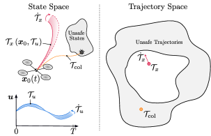
Figure 1: Illustration of trajectory spaces for a quadrotor where $\mathcal{T}_{x}$ represents the current planned trajectory in state space, $\mathcal{T}_{u}$ is the current control input trajectory of length $T$ and $\bm{x}_{0}(t)$ is the current state of the quadrotor. The white set in trajectory space indicates the set of all safe planned trajectories and $\mathcal{T}_{\textrm{col}}$ is an exemplary unsafe trajectory.

We introduce forward invariance in trajectory spaces (FITS), specifically, we

1. overcome reactive behavior of CBFs by considering the future evolution of a system in a trajectory space,

2. propose an efficient QP formulation in the trajectory space that guarantees safety over states proactively, and

3. show in experiments that safety constraints can be enforced without major design effort.

II Related Work

We review two safety-critical control approaches relevant to our approach, namely CBFs and NMPC.

Predictive CBFs [4] have been introduced as a generalization of future-focused CBFs [10] to address the reactive nature of CBFs. The authors consider the evolution of a trajectory under a nominal control law which is allowed to be unsafe. Whenever this trajectory leads to future safety violations, the current control input is modified to proactively avoid unsafe states while assuming no actuation constraints. In contrast, we formulate safe sets in trajectory space that encode both, safety and actuation constraints.

Backup CBFs [11, 12] guarantee the existence of a trajectory that will lead to a control invariant set. Specifically, to ensure future safety, [11] leverages a flow map, i.e. the solution to an initial value problem of an ODE under the safe backup policy. The main difficulty is to find a valid backup policy which typically requires domain specific knowledge. In [13], Hamilton-Jacobi reachability analysis is used to find a valid backup policy. Our approach does not require the definition of a backup policy. Instead, we directly optimize over trajectory changes to ensure future safety.

To combine CBF and RHC approaches, [7] introduced discrete-time CBF conditions as constraints in an NMPC problem. If a valid discrete-time CBF is available, the approach can guarantee safety along a horizon given that the optimization problem is always feasible. An empirical investigation has been carried out in [14] which shows that the CBF condition generally enhances the feasibility. The authors of [6] leverage model predictive safety filters that enforce terminal states of planned trajectories to lie within a control invariant set which is closely related to backup CBFs. However, NMPC tends to be computationally expensive as it requires solving a nonlinear program, leading to the introduction of more efficient yet inexact methods [15, 16, 17].

To overcome the computational burden of NMPC, continuation methods [18, 19] have been introduced for RHC. These methods address problems with equality constraints exclusively by formulating a system of equations to determine the optimal control trajectory. The authors of [18] exploit the recursive structure of RHC and look at the time derivative of the system of equations. This formulation leads to a dynamical system that can be efficiently integrated to obtain a control law. As the continuation method only allows for equality constraints, safety and actuation constraints which are formulated as inequalities cannot be handled. In contrast, we model the planned trajectories as dynamical system which allows for inequality constraints on the trajectory state.

In [5], parameterized trajectory libraries are used to reformulate a RHC problem into a parameter optimization. Finding a trajectory library that satisfies the assumptions of always ending in an equilibrium state [5] is difficult for general nonlinear systems. In our work, we directly optimize for changes in the input trajectory which makes it applicable to a broader class of systems.

III Background

In this section we develop the notation used throughout the paper and present the necessary technical background to formalize the problem.

Consider a general nonlinear control system defined by the ordinary differential equation (ODE)

$$\frac{\mathrm{d}}{\mathrm{d}\tau}\bm{x}_{\tau}=\bm{F}(\bm{x}_{\tau},\bm{u}_{\tau}),$$ (1)

with state $\bm{x}\in\mathcal{X}\subseteq\mathbb{R}^{n_{x}}$, input $\bm{u}\in\mathcal{U}\subseteq\mathbb{R}^{n_{u}}$ and a continuously differentiable deterministic function $\bm{F}:\mathcal{X}\times\mathcal{U}\to\mathbb{R}^{n_{x}}$. By encoding safety through a continuously differentiable constraint function $h:\mathcal{X}\rightarrow\mathbb{R}$, a safe set $\mathcal{C}\subseteq\mathcal{X}$ can be constructed as the 0-superlevel set of $h$ such that

$$\mathcal{C} =\left\{\bm{x}\in\mathcal{X}\mid h\left(\bm{x}\right)\geq 0\right\},$$ (2)

$$\partial\mathcal{C} =\left\{\bm{x}\in\mathcal{X}\mid h\left(\bm{x}\right)=0\right\}.$$

Definition 1.

A safe set $\mathcal{C}$ is forward invariant with respect to the system (1) if for every initial condition $\bm{x}_{\tau_{0}}\in\mathcal{C}$ it holds that $\bm{x}_{\tau}\in\mathcal{C},\forall\tau\geq\tau_{0}$.

A prominent approach in safe control is to render safe sets forward invariant by using CBFs.

Definition 2.

Given a set $\mathcal{C}$, defined by Eq. (2), $h$ serves as a zeroing CBF for the system (1) if for all $\bm{x}$ satisfying $h\left(\bm{x}\right)\geq 0$, there exists a $\bm{u}\in\mathcal{U}$ such that

$$\frac{\mathrm{d}}{\mathrm{d}\tau}h(\bm{x}_{\tau})=\frac{\partial h}{\partial\bm{x}}\left(\bm{F}\left(\bm{x}_{\tau},\bm{u}_{\tau}\right)\right)\geq-\alpha\left(h\left(\bm{x}_{\tau}\right)\right),$$

where $\alpha$ is a class-$\kappa$ function, i.e. continuous and strictly increasing with $\alpha(0)=0$.

If a valid CBF exists, it follows that a controller satisfying Def. 2 renders $\mathcal{C}$ forward invariant [1]. In the case of control affine dynamics of the form $\bm{F}(\bm{x},\bm{u})=\bm{f}\left(\bm{x}\right)+\bm{g}\left(\bm{x}\right)\bm{u}$, we can formulate the control synthesis as quadratic program (QP)

$$\bm{u}_{\tau}^{*}=\operatorname*{arg\,min}_{\bm{u}_{\tau}\in\mathcal{U}} \left(\bm{u}_{\tau}-\bm{u}_{\text{ref}}\right)^{T}{\bm{Q}}\left(\bm{u}_{\tau}-\bm{u}_{\text{ref}}\right)$$ (3)

s.t. $$\frac{\partial h}{\partial\bm{x}}\left(\bm{f}(\bm{x}_{\tau})+\bm{g}(\bm{x}_{\tau})\bm{u}_{\tau}\right)\geq-\alpha(h(\bm{x}_{\tau})),$$

where $\bm{u}_{\text{ref}}$ is a reference controller and $\bm{Q}$ denotes a weighting matrix.

Theorem 1.

If the QP in Eq. (3) is always feasible, the set $\mathcal{C}=\left\{\bm{x}\in\mathcal{X}\mid h\left(\bm{x}\right)\geq 0\right\}$ is forward invariant, i.e. $\bm{x}_{\tau_{0}}\in\mathcal{C}\implies\bm{x}_{\tau}\in\mathcal{C}~{}~{}\forall\tau\geq\tau_{0}$.

For a detailed proof, the reader is referred to [1].

III-A Input and State Trajectories

We define the state trajectory $\mathcal{T}_{x}^{I}$ and the input trajectory $\mathcal{T}_{u}^{I}$ on a closed interval $I=[a,b]$ as

$$\mathcal{T}_{x}^{I} :=\{\bm{x}_{\tau}\in\mathcal{X}\mid\tau\in I\}\in\mathcal{X}^{I}\subseteq L^{2}(I,\mathcal{X})$$

$$\mathcal{T}_{u}^{I} :=\{\bm{u}_{\tau}\in\mathcal{U}\mid\tau\in I\}\in\mathcal{U}^{I}\subseteq L^{2}(I,\mathcal{U}),$$

where $\mathcal{X}^{I}$ and $\mathcal{U}^{I}$ are the sets of possible trajectories that are also square integrable ($L^{2}$) on the interval $I$.

A state $\bm{x}_{\tau}$ at time $\tau\in I$ is fully determined by the dynamics (1), the initial condition $\bm{x}_{a}\in\mathcal{X}$ and the input trajectory $\mathcal{T}_{u}^{[a,\tau]}$ as

$$\bm{x}_{\tau}=\varphi\left(\bm{x}_{a},\mathcal{T}_{u}^{[a,\tau]}\right)\coloneq\bm{x}_{a}+\int_{a}^{\tau}\bm{F}\left(\bm{x}_{\tilde{\tau}},\bm{u}_{\tilde{\tau}}\right)\mathrm{d}\tilde{\tau},$$ (4)

thus the state trajectory can be obtained by integrating the ODE in Eq. (1), i.e.

$$\mathcal{T}_{x}^{I} =\left\{\varphi\left(\bm{x}_{a},\mathcal{T}_{u}^{[a,\tau]}\right)\in\mathcal{X}\mathrel{\Big{|}}\tau\in I\right\}.$$

Note that state trajectories are continuous, i.e. $\mathcal{X}^{I}\subseteq C^{0}(I,\mathcal{X})$ for any square integrable input trajectory, which follows from the continuous differentiability assumption on the dynamics (1).

We introduce the variable $t$ to denote system time which describes the temporal evolution in the real world. In contrast, we use trajectory time $\tau$, to describe the time evolution of a state $\bm{x}_{\tau}$ along a state trajectory $\mathcal{T}_{x}^{I}$ within the interval $I$.

Consequently, the state and input trajectories become a function of system time, i.e. $\mathcal{T}_{x}^{I}(t)$ and $\mathcal{T}_{u}^{I}(t)$, respectively. Figure 2 illustrates a one-dimensional example of a state trajectory $\mathcal{T}_{x}^{I}(t)$ varying over system time $t$. In the remainder of this paper, we use subscripts, i.e. $\bm{x}_{\tau}$, to denote trajectory time and parentheses, i.e. $\bm{x}(t)$, to denote system time. As also visualized in Figure 2, the state $x_{\tau_{p}}(t_{p})$ denotes the state at system time $t_{p}$ and trajectory time $\tau_{p}$.

IV Problem Statement

A trajectory $\mathcal{T}_{x}^{I}(t)$ that is planned in a receding horizon fashion should be safe at all times $t$ which we formally define hereafter.

Problem 1.

Given a dynamical system in Eq. (1) and a planning horizon $I=[0,T]$, ensure that $\forall t\geq 0$

$$h_{i}(\bm{x}_{\tau}) \geq 0,~{}\forall i=0,\dots,m-1,\forall\bm{x}_{\tau}\in\mathcal{T}^{I}_{x}(t),$$ (5)

$$\bm{u}_{\mathrm{min}} \leq\bm{u}_{\tau}\leq\bm{u}_{\mathrm{max}}\hskip 46.09332pt\forall\bm{u}_{\tau}\in\mathcal{T}^{I}_{u}(t),$$ (6)

where $m$ inequality constraints encode safety specifications and Eq. (6) denotes actuation constraints.

We want to solve this problem through the framework of control barrier functions to benefit from their formal guarantees. To that end, we lift the problem to the trajectory space, i.e. the space of all possible planned trajectories.

IV-A Trajectory Space Dynamics

We introduce the continuous-time dynamics of trajectories $\mathcal{T}_{x}^{I}$ and $\mathcal{T}_{u}^{I}$, respectively.

To study the change of the trajectories over time we introduce the derivative along system time $t$ of the corresponding state trajectory $\mathcal{T}_{x}^{I}(t)$, reading

$$\dot{\mathcal{T}}_{x}^{I}(t) \coloneq\left\{\frac{\mathrm{d}}{\mathrm{d}t}\varphi\left(\bm{x}_{0}(t),\mathcal{T}_{u}^{[0,\tau]}(t)\right)\mathrel{\Big{|}}\tau\in I\right\}$$ (7)

$$=\left\{\frac{\partial\varphi}{\partial\bm{x}_{0}(t)}\dot{\bm{x}}_{0}(t)+\int_{0}^{\tau}\frac{\partial\varphi}{\partial\bm{u}_{\hat{\tau}}(t)}\dot{\bm{u}}_{\hat{\tau}}(t)\,\mathrm{d}\hat{\tau}\mathrel{\Big{|}}\tau\in I\right\}$$ (8)

$$\dot{\mathcal{T}}_{u}^{I}(t) =\mathcal{T}_{v}^{I}(t)=\left\{\bm{v}_{\tau}(t)\in\mathbb{R}^{n_{u}}\mid\tau\in I\right\}\in\mathcal{V}^{I},$$ (9)

where we use the ${(\cdot)}$ notation for the derivative with respect to actual time $t$, and $\mathcal{T}_{v}^{I}$ denotes the trajectory of a virtual input $\bm{v}$. This virtual input controls the rate of change of the input trajectory, i.e. $\dot{\bm{u}}_{\tau}(t)=\bm{v}_{\tau}(t)$. The existence of the partial derivatives in the definition (8) follows from the assumption on continuously differentiable dynamics (1).

Thus, we view the planned trajectories $\mathcal{T}_{x}^{I}$ and $\mathcal{T}_{u}^{I}$ as dynamical systems that we can affect through the virtual input $\bm{v}$. Having introduced this dynamical system, we can reformulate the original problem as follows.

Problem 2.

Given the dynamical system of trajectories in Eq. (7)-(9) and safety constraints (5)-(6), find a safe set $\mathcal{C}$ in trajectory space $\mathcal{X}\times\mathcal{U}^{I}$ and a corresponding control law $\pi_{v}:\mathcal{X}\times\mathcal{U}^{I}\mapsto\mathcal{V}^{I}$ that ensures the satisfaction of safety constraints by rendering the safe set forward invariant.

By solving Problem 2, we ensure that the planned trajectories remain in a safe set in trajectory space at all times which, in turn, would solve Problem 1.

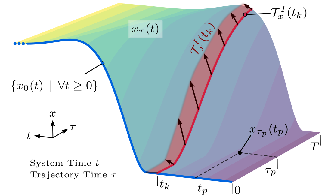
Figure 2: Notation used for time variables and the trajectory space dynamics for a one-dimensional state space example. The surface color changes along the system time $t$. We denote by $x_{\tau_{p}}(t_{p})$ the state at system time $t_{p}$ and trajectory time $\tau_{p}$. The time derivative of the state trajectory at time $t_{k}$ within the planning interval, i.e., $\dot{\mathcal{T}}_{x}^{I}(t_{k})$, is shown as a vector field (shaded in red) on the corresponding state trajectory $\mathcal{T}_{x}^{I}(t_{k})$. The executed trajectory $\{x_{0}(t)\mid\forall t\geq 0\}$ is shown in blue.

V Forward Invariance in Trajectory Spaces

To solve the aforementioned problem, we introduce Forward Invariance in Trajectory Spaces (FITS) which treats receding horizon control as a dynamical system in the trajectory space. Our approach can be summarized as follows: We 1) define a trajectory configuration space $\mathcal{S}$ with a finite dimensional state $\bm{s}\in\mathcal{S}$ that uniquely describes the current planned trajectory $\mathcal{T}_{x}^{I}$ and obtain its dynamics, 2) we convert the original safety and actuation constraints into sets in the space $\mathcal{S}$ and 3) we ensure that these sets are forward invariant.

V-A Trajectory State Parameterization

We introduced the dynamics of planned trajectories as a dynamical system over continuous functions in Eq. (7)-(9) which describes an infinite dimensional dynamical system. Therefore, the goal of this section is to find a finite representation that we can use for control design.

We consider piecewise constant input trajectories of $N$ steps on the interval $I=[0,T]$

$$\mathcal{T}_{u}^{I}(t)=\left\{\bm{u}_{i}\mid\forall\tau\in[\tau_{i},\tau_{i+1}),\forall i=0,\dots,N-1\right\}\in\mathcal{U}^{I}$$

where $\bm{u}_{i}\in\mathcal{U}$ is the input applied within the $i$th step, each for a duration of $\delta\tau=\nicefrac{{T}}{{N}}$. Following this parameterization of an input trajectory, we define the state

$$\bm{s}(t):=\begin{bmatrix}\bm{x}_{0}(t)&\bm{u}_{0}(t)&\dots&\bm{u}_{N-1}(t)\end{bmatrix}^{T}\in\mathcal{S}\subseteq\mathcal{X}\times\mathcal{U}^{N},$$ (10)

that uniquely describes the current planned trajectory $\mathcal{T}_{x}^{I}(t)$ since it only depends on the initial conditions $\bm{x}_{0}(t)$ and the input trajectory $\mathcal{T}_{u}^{I}(t)$.

Next, we define a dynamical system that describes the evolution of $\bm{s}$. The state of the robotic system $\bm{x}_{0}(t)$ is always the initial state for a planned trajectory $\mathcal{T}_{x}^{I}(t)$. Thus, its total derivative wrt. system time is given by the dynamics model (1), i.e. $\dot{\bm{x}}_{0}(t)=\bm{F}({\bm{x}}_{0}(t),{\bm{u}}_{0}(t))$. Since the control input trajectory is a decision variable that we can change over time, we model it as a single integrator, i.e. $\dot{\bm{u}}_{i}=\bm{v}_{i}$ where $\bm{v}_{i}$ is a virtual input.

In summary, a trajectory state $\bm{s}\in\mathcal{S}$ evolves according to

$$\dot{\bm{s}} =\begin{bmatrix}\bm{F}(\bm{x}_{0},\bm{u}_{0})\\ \bm{0}\end{bmatrix}+\begin{bmatrix}\bm{0}\\ \bm{I}\end{bmatrix}\bm{v}$$ (11)

$$=\bm{f}_{s}(\bm{s})+\bm{g}_{s}(\bm{s})\bm{v}$$ (12)

where $\bm{v}\in\mathbb{R}^{n_{u}\cdot N}$. Interestingly, even though the dynamics of $\bm{x}$ do not need to be control affine, the dynamics of the trajectory state are affine in $\bm{v}$.

V-B State Constraints as Safe Set in Trajectory Space

In this section, we describe how the safety constraints in Eq. (5) can be converted into a set $\mathcal{C}_{h}\subseteq\mathcal{S}$ that, if forward invariant, ensures that the original constraints hold. The main difficulty lies in the fact that safety constraints are defined over physical states $\bm{x}$ while $\mathcal{S}$ only contains the initial physical state $\bm{x}_{0}$ and a piecewise constant input trajectory $\mathcal{T}_{u}^{I}$.

Given a current trajectory state $\bm{s}$, we can leverage the mapping $\varphi$ defined in Eq. (4), to map a state $\bm{s}$ to a physical state $\bm{x}_{\tau}$ on the trajectory $\mathcal{T}_{x}^{I}$, reading

$$\bm{x}_{\tau}=\varphi\left(\bm{x}_{0},\mathcal{T}_{u}^{[0,\tau]}\right)=\varphi(\bm{s},\tau).$$ (13)

Thus from a state $\bm{s}$ we can uniquely obtain a continuous time trajectory $\mathcal{T}_{x}^{I}$ by solving the ODE in Eq. (1) given the initial state and the continuous-time input trajectory. More importantly, we can leverage efficient differentiable ODE solvers [20] to also obtain the Jacobian $\nicefrac{{\partial{\varphi}}}{{\partial\bm{s}}}$.

Next, we can define a set in the trajectory configuration space $\mathcal{S}$ that encodes the constraints in Eq. (5) as

$$\mathcal{C}_{h}=\left\{\bm{s}\in\mathcal{S}\mid h_{i}(\varphi(\bm{s},\tau))\geq 0,\hskip 5.69046pt\forall\tau\in I,\forall i=0,\dots,m-1\right\}$$

since the physical state $\bm{x}_{\tau}$ is explicitly expressed as a function of the state $\bm{s}$ through the mapping $\varphi$.

Assumption 1.

We consider a discretized solution of $\bm{x}_{\tau}$ at times $\tau_{0},\dots,\tau_{M-1}$ where $\tau_{0}=0$ and $\tau_{M-1}=T$, respectively. We assume that it is sufficient to consider constraints at discrete time steps along the planned trajectory $\mathcal{T}_{x}^{I}$, i.e.

$$\mathcal{C}_{h}=\bigcap_{j=0}^{M-1}\left\{\bm{s}\in\mathcal{S}\mid h_{i}(\varphi(\bm{s},\tau_{j}))\geq 0,\hskip 5.69046pt\forall i=0,\dots,m-1\right\}.$$

While this approximation does not recover the original safe set over continuous trajectories, we can get arbitrarily close by increasing the number of time steps considered. Further, we leave it for future work to find Lipschitz arguments to relax Assumption 1.

To ensure that a planned trajectory will satisfy safety constraints at all times, we formulate a CBF condition in trajectory configuration space $\mathcal{S}$.

Lemma 1.

If for all $\bm{s}\in\mathcal{C}_{h}$, there exists a locally Lipschitz virtual input $\bm{v}\in\mathbb{R}^{n_{u}\cdot N}$ and a class-$\kappa$ function $\alpha_{1}$ such that $\forall i=0,\dots,m-1$ (constraints) and $\forall j=0,\dots,M-1$ (time steps)

$$\frac{\mathrm{d}}{\mathrm{d}t}\left(h_{i}(\varphi_{j})\right) =\frac{\partial h_{i}}{\partial\bm{x}}\frac{\partial\varphi_{j}}{\partial\bm{s}}\left(\frac{\mathrm{d}}{\mathrm{d}t}\bm{s}\right)$$ (14)

$$=\frac{\partial h_{i}}{\partial\bm{x}}\frac{\partial\varphi_{j}}{\partial\bm{s}}\left(\bm{f}_{s}(\bm{s})+\bm{g}_{s}(\bm{s})\bm{v}\right)$$

$$\geq-\alpha_{1}\left(h_{i}(\varphi_{j})\right)$$

with $\varphi_{j}=\varphi(\bm{s},\tau_{j})$ holds, then $\mathcal{C}_{h}$ is forward invariant.

The proof follows analogously to the proof of forward invariance of zeroing CBFs in Theorem 1, proposed in [1]. Importantly, the invariance of $\mathcal{C}_{h}$ implies that the inequality constraints over physical states in Eq. (5) holds at all times.

Remark 1.

While the continuous-time physical state trajectory $\mathcal{T}_{x}^{I}(\bm{s})$ can have points of non-smoothness, every point on the trajectory $\bm{x}_{\tau_{i}}=\varphi(\bm{s},\tau_{i})$ is continuously differentiable with respect to the state $\bm{s}$. This is necessary for the invariance result and follows from the continuously differentiable dynamics model (1).

V-C Actuation Constraints

In order to ensure safety in real-world settings, we also need to consider actuation constraints of robots. In FITS, actuation constraints can be interpreted as sets in $\mathcal{S}$ that we want to render forward invariant since the control input $\bm{u}$ is part of the state $\bm{s}$.

Similar to the considered safety constraints, we can directly define sets in $\mathcal{S}$ that ensure actuation constraints to be satisfied, i.e.

$$\mathcal{C}_{\mathrm{min}} =\left\{\bm{s}\in\mathcal{S}\mid\bm{h}_{\mathrm{min}}(\bm{s})\geq\bm{0}\right\}$$

$$\mathcal{C}_{\mathrm{max}} =\left\{\bm{s}\in\mathcal{S}\mid\bm{h}_{\mathrm{max}}(\bm{s})\geq\bm{0}\right\},$$

where $\bm{h}_{\mathrm{min}}=[(\bm{u}_{0}-\bm{u}_{\mathrm{min}})~{}\dots~{}(\bm{u}_{N-1}-\bm{u}_{\mathrm{min}})]^{T}$ and $\bm{h}_{\mathrm{max}}=[(\bm{u}_{\mathrm{max}}-\bm{u}_{0})~{}\dots~{}(\bm{u}_{\mathrm{max}}-\bm{u}_{N-1})]^{T}$. Thus, to satisfy actuation constraints, we need to ensure that there exists a virtual input $\bm{v}$ such that $\forall k=0,\dots,n_{u}\cdot N-1$

$$\frac{\mathrm{d}}{\mathrm{d}t}\left(h_{\mathrm{min}}^{(k)}(\bm{s})\right) =\frac{\partial h_{\mathrm{min}}^{(k)}}{\partial\bm{s}}\left(\bm{f}_{s}(\bm{s})+\bm{g}_{s}(\bm{s})\bm{v}\right)$$ (15)

$$\geq-\alpha_{2}\left(h_{\mathrm{min}}^{(k)}(\bm{s})\right)$$

holds, where $\alpha_{2}$ is a class-$\kappa$ function and $h_{\mathrm{min}}^{(k)}$ is the $k$th entry of $\bm{h}_{\mathrm{min}}$. The condition for the maximum actuation constraints follows analogously.

V-D Incorporating an Objective

Contrary to standard CBF-QP formulations as in Eq. (3), FITS does not need an explicit reference controller and can directly incorporate a cost function that, e.g., encodes desired tracking performance.

For a given state $\bm{s}$, we can reconstruct both, the input trajectory $\mathcal{T}_{u}^{I}$ and the state trajectory $\mathcal{T}_{x}^{I}$. Thus, we can define an objective function over input and state trajectories as $J=J(\mathcal{T}_{x}^{I},\mathcal{T}_{u}^{I})=J(\bm{s})$. More importantly, if $J$ is differentiable, we can evaluate the time derivative of the objective function as

$$\frac{\mathrm{d}}{\mathrm{d}t}J(\bm{s})=\frac{\partial J}{\partial\bm{s}}\dot{\bm{s}}=\frac{\partial J}{\partial\bm{s}}\left(\bm{f}_{s}(\bm{s})+\bm{g}_{s}(\bm{s})\bm{v}\right),$$ (16)

meaning that we can affect the control trajectory via $\bm{v}$ such that the objective will be minimized over time. Generally, the objective function can encode any desired behavior as function of states and inputs but we can also recover the same objective as in Eq. (3) where the deviation of a reference controller is minimized.

V-E Control Synthesis in Trajectory Spaces

This leads us to our final formulation of FITS in which we optimize for a virtual input $\bm{v}$ that minimizes an objective function over time while satisfying actuation and safety constraints.

Given an initial state $\bm{s}$ composed of the initial physical state $\bm{x}_{0}(t_{0})$ as well as an initial input trajectory $\mathcal{T}_{u}^{I}(t_{0})$, we synthesize virtual inputs $\bm{v}$ by solving

$$\min_{\bm{v}} \bm{v}^{T}\bm{Q}\bm{v}+\frac{\partial J}{\partial\bm{s}}\bm{g}_{s}(\bm{s})\bm{v}$$ (17)

s.t. $$\frac{\partial h_{i}(\varphi_{j})}{\partial\bm{s}}\left(\bm{f}_{s}(\bm{s})+\bm{g}_{s}(\bm{s})\bm{v}\right)\geq-\alpha_{1}\left(h_{i}(\varphi_{j})\right)$$

$$\frac{\partial h_{\mathrm{min}}^{(k)}}{\partial\bm{s}}\left(\bm{f}_{s}(\bm{s})+\bm{g}_{s}(\bm{s})\bm{v}\right)\geq-\alpha_{2}\left(h_{\mathrm{min}}^{(k)}(\bm{s})\right)$$

$$\frac{\partial h_{\mathrm{max}}^{(k)}}{\partial\bm{s}}\left(\bm{f}_{s}(\bm{s})+\bm{g}_{s}(\bm{s})\bm{v}\right)\geq-\alpha_{2}\left(h_{\mathrm{max}}^{(k)}(\bm{s})\right)$$

with $\varphi_{j}\coloneq\varphi(\bm{s},\tau_{j})$, $i=0,\dots,m-1$, $j=0,\dots,M-1$ and $k=0,\dots,n_{u}\cdot N-1$. Note that the optimization problem (17) is quadratic in $\bm{v}$ and, thus, can be solved efficiently using off-the-shelf QP solvers. The additive quadratic term in $\bm{v}$ with a positive definite matrix $\bm{Q}$ reduces the rate of change of the input trajectory over time, inducing a smoother change in trajectories. To connect our method back to the problem statement, the QP in Eq. (17) is a control law $\pi_{v}:\mathcal{S}\to\mathcal{V}^{I}$ that we propose as solution to Problem 2.

VI Analysis

We now have the necessary elements to discuss the theoretical properties of FITS.

Theorem 2.

Consider the dynamical system in Eq. (1), the safety constraints in Eq. (5) and the actuation constraints in Eq. (6). If the control input sequence evolves according to

$$\dot{\bm{u}}_{i}=\bm{v}_{i}^{*},\hskip 5.69046pt\forall i=0,\dots,N-1$$

where $\bm{v}^{*}$ is the solution to Eq. (17), then all inequality constraints (14) and actuation constraints (15) will be satisfied at all times $t\geq t_{0}$, given that $\bm{s}(t_{0})\in\mathcal{C}_{h}\cap\mathcal{C}_{\textrm{min}}\cap\mathcal{C}_{\textrm{max}}$.

Proof.

If the QP is always feasible, Eq. (14) always holds, implying that the set $\mathcal{C}_{h}$ is forward invariant. Similarly, the sets defining the actuation constraints, $\mathcal{C}_{\mathrm{min}}$ and $\mathcal{C}_{\mathrm{max}}$, are rendered forward invariant through Eq. (15) and, thus, actuation constraints are satisfied at all times, see Thm. 1. ∎

VI-A Feasibility of the QP

In FITS, proving recursive feasibility is different than in general input-constrained CBF-QPs. We have to show that multiple safe sets are control-sharing since all sets are defined in the same space and can be affected via $\bm{v}$. Here, control-sharing means that the individual CBF conditions of safety and actuation are non-conflicting. However, so far there is only work for single input systems that rigorously provides a controller with feasibility guarantees for multiple defined safe sets [21].

Below, we show the necessary conditions for the QP to be feasible.

Theorem 3.

The QP in Eq. (17) is always feasible if and only if

$$\sum_{k}\lambda_{k}\frac{\partial h_{k}}{\partial\bm{s}}\bm{g}_{s}=\bm{0}\implies\sum_{k}\lambda_{k}\left(\frac{\partial h_{k}}{\partial\bm{s}}\bm{f}_{s}+\alpha(h_{k}(\bm{s}))\right)\geq 0$$ (18)

holds for each individual constraint in Eq. (17), i.e. $k=1,\dots,m\cdot M+2\cdot n_{u}\cdot N$ and for all $\bm{s}\in\mathcal{C}_{h}\cap\mathcal{C}_{\textrm{min}}\cap\mathcal{C}_{\textrm{max}}$ and for all $\lambda_{k}\geq 0$.

Proof.

Consider the feasibility problem of the QP in Eq. (17) which is characterized by the Lagrangian

$$\mathcal{L}(\bm{s},\bm{v},\bm{\lambda})=-\sum_{k}\lambda_{k}\left(\frac{\partial h_{k}}{\partial\bm{s}}\bm{g}_{s}\bm{v}+\frac{\partial h_{k}}{\partial\bm{s}}\bm{f}_{s}+\alpha(h_{k}(\bm{s}))\right).$$

If there exists a $\bm{v}\in\mathbb{R}^{n_{u}\cdot N}$ for all non-negative Lagrange multipliers $\bm{\lambda}\geq\bm{0}$ such that the complementary slackness condition $\mathcal{L}(\bm{s},\bm{v},\bm{\lambda})\leq 0$ is satisfied, the QP is feasible for a given state $\bm{s}\in\mathcal{S}$ [22].

If Eq. (18) holds, it follows directly that $\mathcal{L}\leq 0$ if $\sum_{k}\lambda_{k}(\nicefrac{{\partial h_{k}}}{{\partial\bm{s}}})\bm{g}_{s}=\bm{0}$ holds. Otherwise, it follows that the Lagrange dual function results in $\mathrm{inf}_{\bm{v}}~{}\mathcal{L}(\bm{s},\bm{v},\bm{\lambda})=-\infty$ which concludes that Eq. (18) implies feasibility of the QP for a given state $\bm{s}$. Since Eq. (18) holds for all $\bm{s}\in\mathcal{C}_{h}\cap\mathcal{C}_{\textrm{min}}\cap\mathcal{C}_{\textrm{max}}$, the QP is feasible for all $t\geq t_{0}$ given that $\bm{s}(t_{0})\in\mathcal{C}_{h}\cap\mathcal{C}_{\textrm{min}}\cap\mathcal{C}_{\textrm{max}}$ since $\mathcal{C}_{h}\cap\mathcal{C}_{\textrm{min}}\cap\mathcal{C}_{\textrm{max}}$ is forward invariant (see Thm. 2). ∎

In words, Thm. 3 requires the uncontrolled solution of $\bm{s}$ according to the drift term $\bm{f}_{s}(\bm{s})$ to still satisfies the CBF conditions in critical points in which the effect of the virtual input $\bm{v}$ on the constraint function vanishes.

VI-B Discrete-time Implementation

So far, we have assumed that the control synthesis problem in trajectory spaces can be solved in continuous time. However, although QPs can be solved efficiently, there will always be a limited control rate of the presented method. Therefore, we draw motivation from existing works on CBFs in sampled-data systems [23].

Assuming a zero-order-hold (ZOH) controller, i.e. $\forall t\in[t_{k},t_{k}+\delta t)$

$$\dot{\mathcal{T}}_{u}(t)=\left\{\bm{v}_{i}(t_{k})\mid\forall\tau\in[\tau_{i},\tau_{i+1}),\hskip 2.84544pt\forall i=0,\dots,N-1\right\},$$

we can modify the obtained CBF conditions to account for the worst-case evolution in between time steps $\delta t$. To that end, we can modify the right-hand-side (RHS) of Eq. (14) and (15) to include an additional term of the form

$$RHS:=-\alpha\left(h(\bm{s})\right)+\nu\left(\delta t,\bm{s}\right)$$

where $\nu$ is typically a function of Lipschitz constants of the dynamical system as well as the sampling time $\delta t$. One instantiation of $\nu$ is presented in [23] based on global Lipschitz constants of dynamics and constraint functions.

Although this approach enforces the forward invariance, the Lipschitz constants for high-dimensional trajectory space dynamics are generally hard to compute and lead to overly conservative behavior.

In practice, we aim to ensure that $h(\bm{s}(t_{k}+\delta t))\geq 0$ for any $t_{k}\geq t_{0}$ given $h(\bm{s}(t_{0}))\geq 0$. Approximating $h(\bm{s}(t_{k}+\delta t))$ by a first order estimate and using $h(t)=h(\bm{s}(t))$, we obtain

$$h(t_{k}+\delta t)\approx h(t_{k})+\dot{h}(t_{k})\delta t\geq 0$$

$$\Leftrightarrow\dot{h}(t_{k})\geq-\frac{1}{\delta t}h(t_{k}),$$

where the estimate becomes exact as $\delta t\to 0$. When the approximation is good enough with a given $\delta t>0$, we obtain an upper bound for the class-$\kappa$ functions $\alpha(x)$ in the inequality constraints (14) and (15) as

$$\dot{h}(t_{k})\geq-\alpha(h(t_{k}))\geq-\frac{1}{\delta t}h(t_{k}).$$

Therefore, with real-time control ($\delta t\leq$0.01\text{\,}\mathrm{s}$$) of mechanical systems that tend to be much slower, choosing $\alpha(h)\ll\frac{1}{\delta t}h$ is likely a safe choice.

VI-C Limitations

Our proposed method has two main limitations: 1) The provided guarantees hold in the limit as the replanning step approaches zero and 2) our method can be considered to be a shooting method, thus, FITS can have high sensitivity in the gradients for long planning horizons.

As discussed in section VI-B, we can obtain Lipschitz arguments to account for the worst-case evolution assuming a ZOH discretization to address the first limitation. While this seems promising, it is also difficult to find tight Lipschitz arguments for these high-dimensional systems.

For the latter limitation, we can draw motivation from multiple shooting optimization methods which address the problem of gradient sensitivity. It might be possible to split the overall optimization problem into multiple smaller ones and enforce continuity between the optimized trajectories. We are planning to address both limitations in future work.

VII Connections to I-CBFs and NMPC

In this section, we discuss how FITS is related to different control strategies, namely Integral CBFs (I-CBFs) and Sequential Quadratic Programming (NMPC-SQP). We present different angles on the control synthesis problem and position FITS in relation to other methods.

VII-A Integral Control Barrier Functions

I-CBFs[24] were introduced for the coupled dynamical system

$$\begin{bmatrix}\dot{\bm{x}}\\ \dot{\bm{u}}\end{bmatrix}=\begin{bmatrix}\bm{F}(\bm{x},\bm{u})\\ \phi(\bm{x},\bm{u},t)+\bm{v}\end{bmatrix}$$

where $\bm{u},\bm{v}\in\mathbb{R}^{n_{u}}$ and $\phi$ is a general feedback control law. Similar to FITS, the authors rely on a control law through a virtual input $\bm{v}$. The main difference to FITS lies in the fact that we consider an input trajectory $\mathcal{T}^{I}_{u}$ instead of just one control input. Therefore, our method overcomes the short-sightedness of I-CBFs by incorporating a planning horizon.

The authors in [24] formulate a QP with $\bm{v}$ as decision variable to ensure forward invariance of a safe set $\mathcal{C}$, also incorporating input constraints. In FITS, we can view the unconstrained minimization of $\dot{J}(\bm{s})$ in Eq. (16) as the general feedback law $\phi$ which describes a gradient descent policy on the objective function $J$. We recover the exact I-CBF formulation by reducing the planning horizon to a single control input $\bm{u}_{0}$, resulting in a myopic control law.

VII-B Sequential Quadratic Programming for NMPC

The discrete implementation of FITS is tightly connected to real-time iteration NMPC-SQP methods [16, 17, 15]. Both are solving a quadratic program at each iteration. FITS solves for rates; SQP solves for deltas. One way how discrete FITS steps generalize SQP iterates, is that the latter use linearized constraints which resemble the CBF inequality constraints in Eq. (14) with a fixed class-$\kappa$ function $\alpha(h)=1\cdot h$.

While SQP iterates are not ensured to remain safe, its iterates are equivalent to the discrete FITS steps when using a constant symmetric positive definite (SPD) hessian approximation and the above choice of class-$\kappa$ function. Following the analysis in Sec. VI-B, our work provides insight into when real-time iteration NMPC-SQP methods ensure safety in practice, since the iteration time is low and the linearized constraint function resembles a CBF constraint.

VIII Experiments

In this section, we evaluate FITS in safety-critical scenarios in which a planning horizon is crucial. Specifically, we show

1. adherence to safety specifications while not sacrificing performance in Sec. VIII-B

2. that FITS overcomes the purely reactive behavior of CBFs in Sec. VIII-C.

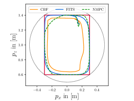
Figure 3: A two-dimensional quadrotor tracking task. The dotted black circle depicts the circular trajectory that we want to track while the red rectangle shows the constrained area that we want to remain in.

VIII-A Setup

To analyze FITS, we run experiments in the common benchmark simulation environment safe-control-gym [25] which offers multiple scenarios for control of nonlinear systems under safety constraints. Specifically, we consider a quadrotor tracking task as well as a custom designed navigation task in a cluttered environment.

We consider two baselines, namely (CBF) a vanilla second order CBF in combination with an LQR reference controller and (NMPC) a nonlinear model predictive controller that recursively solves an optimization problem to obtain a discrete-time control sequence. We use the available implementation in [25] which is based on CasADi’s opti framework to formulate the optimization problem which is then solved with the interior point method IPOPT.

For our method, we use JAX [26] for efficient auto differentiation to implement the differentiable integrator $\varphi$ in Eq. (4) as an Euler integration scheme. Further, we use cvxopt to solve the QP in Eq. (17). All calculations (including auto differentiation) are carried out on an Intel i9-10900K processor and 32 GB of RAM.

VIII-B Quadrotor Geofencing

In the first experiment, we consider a circular trajectory tracking task of a planar quadrotor subject to a geofencing constraint of staying within a rectangular area as shown in Fig. 3. The state of the robot is given as $\bm{x}=[p_{x}~{}p_{z}~{}\theta~{}\dot{p}_{x}~{}\dot{p}_{z}~{}\dot{\theta}]^{T}$ and the control inputs are two thruster forces $\bm{u}=[F_{1}~{}F_{2}]^{T}$. A detailed description of the equations of motion can be found in [25]. The objective is of linear quadratic form

$$J\left(\mathcal{T}_{x}^{I},\mathcal{T}_{u}^{I}\right)=\int_{0}^{T}\Delta\bm{x}_{\tilde{\tau}}^{T}\bm{Q}_{J}\Delta\bm{x}_{\tilde{\tau}}+\Delta\bm{u}_{\tilde{\tau}}^{T}\bm{R}_{J}\Delta\bm{u}_{\tilde{\tau}}\text{d}\tilde{\tau}$$ (19)

where $\Delta\bm{x}_{\tilde{\tau}}=\bm{x}_{\tilde{\tau}}-\bm{x}_{\textrm{ref}}$ and $\Delta\bm{u}_{\tilde{\tau}}=\bm{u}_{\tilde{\tau}}-\bm{u}_{\textrm{ref}}$, respectively. The safety objective is encoded as

$$h_{i}(\bm{x})=\bm{a}_{i}^{T}\bm{x}-b_{i}\geq 0,\hskip 5.69046pti=1,\dots,4$$ (20)

which represent the four halfspace constraints and actuation constraints are set to $F_{i}\in[0.056,0.297]~{}\text{N}$. For the CBF baseline, we use the CBF design proposed in [27] which specifically deals with obstacle avoidance for planar quadrotors by explicitly including an angular dependency.

In both, NMPC and FITS, we optimize over $N=20$ control steps where each control input is applied for $\delta\tau=1/100\text{s}$. The continuous state trajectory in FITS is discretized into $M=40$ states and the class-$\kappa$ functions in Eq. (17) are chosen as $\alpha_{1}(x)=\alpha_{2}(x)=5x$ which satisfy the practical conditions obtained in Sec. VI-B. In experiments, we noticed that NMPC sometimes becomes infeasible which is why we had to introduce slack variables on the constraints in Eq. (20).

TABLE I: Comparison of FITS to baselines.

	RMSE in [m] $\mu\pm\sigma$	$t_{\text{comp}}$ in [ms] $(\mu\pm\sigma)$	$\lVert\bm{u}\rVert_{2}$ in [N] $(\mu\pm\sigma)$	#violations	$h_{\textrm{min}}$ in [mm]
FITS	$0.157\pm$ $0.075$	$3.2\pm$ 2.5	$0.189\pm$ $0.032$	0	0.2
CBF	$0.27\pm$ $0.04$	$1.22\pm$ 0.3	$0.21\pm$ $0.07$	0	43
NMPC	$0.153\pm$ $0.074$	$98.3\pm$ 7.8	$0.188\pm$ $0.06$	27	-0.09

Figure 3 shows the resulting trajectories for FITS and the baselines. FITS and CBF can ensure safety at all times which is further supported by Table I. However, CBF is overly conservative and does not approach the boundaries of the safe set which results in poor tracking performance as indicated by a large root mean squared error (RMSE) on the tracked circular trajectory. While it looks like NMPC satisfies safety constraints, violation occurs numerous times due to the slack variables in the optimization problem with a maximum violation of $0.09$$\mathrm{m}\mathrm{m}$. FITS satisfies safety and input constraints at all times while achieving similar performance to NMPC in terms of tracking, as indicated by the RMSE, and control effort evaluated as the mean applied force.

Apart from adhering to safety specifications, we observed the following two points that are worth highlighting:

1. In the design process of safety functions for FITS, we neither explicitly accounted for higher relative degrees nor for the underactuation of the system since we directly used Eq. (20) as candidate functions. The baseline CBF proposed in [27] is a second order CBF modified for the specific use case of planar quadrotors.

2. The computation time of FITS was an order of magnitude lower than NMPC and could be run at 200 Hz since it only involved solving a single QP.

VIII-C Navigation in Cluttered Environments

In this section, we consider a navigation task of a double integrator system that is described by the dynamical system $[\dot{p}_{x}~{}\dot{p}_{y}~{}\ddot{p}_{x}~{}\ddot{p}_{y}]^{T}=[\dot{p}_{x}~{}\dot{p}_{y}~{}u_{x}~{}u_{y}]^{T}$. In this scenario, the robot has a goal reaching task while avoiding 30 circular obstacles as depicted in Fig. 4. The cost is defined as in Eq. (19) and safety is encoded as

$$h_{i}\left(\bm{x}\right)=\lVert[p_{x}~{}p_{y}]^{T}-\bm{p}_{o}^{(i)}\rVert_{2}-r_{o}^{(i)},\hskip 8.5359pt\forall i=1,\dots,30$$ (21)

where each obstacle is defined by its position $\bm{p}_{o}$ and its radius $r_{o}$. The actuation limits are $u_{x},u_{y}\in[-1,1]$ and the simulation time is $t_{\textrm{sim}}=8$ seconds.

In this simulation, we consider two CBFs with different class-$\kappa$ functions $\alpha_{1}(x)=20x$ and $\alpha_{2}(x)=2x$. It can be observed that FITS and NMPC are able to reach the goal in the limited time frame while both CBFs get stuck. Interestingly, the more conservative CBF $\alpha_{2}$ avoids getting stuck directly but moves slowly through the environment because the low value of $\alpha_{2}$ results in more conservative behavior. NMPC, on the other hand, manages to find a path through the obstacles but violates safety specifications multiple times due to slack variables in the optimization problem. Specifically, the minimum value of the safety functions in Eq. (21) is $h=-0.026$$\mathrm{m}$ while both, CBF and FITS, keep the state safe at all times.

IX Conclusion and Future Work

In this work, we introduce forward invariance in trajectory spaces (FITS) as an approach to safety-critical control. We model planned trajectories as a dynamical system in a trajectory configuration space $\mathcal{S}$ and define safe sets in this space that encode safety of physical states and actuation constraints. We find an efficient QP formulation for continuous-time receding horizon control by defining CBFs in the space $\mathcal{S}$ that guarantees safe evolution of planned trajectories. Consequently, by incorporating a planning horizon, we overcome purely reactive behavior of standard CBF-QP formulations. Experimental results indicate that we achieve adherence to safety specifications while offering a considerable speedup in computation time compared to an interior point NMPC. Future work will focus on the limitations pointed out in Sec. VI-C, namely the problem of missing rigorous guarantees for discrete-time implementations and on the gradient sensitivity of FITS for long planning horizons. Lastly, with FITS, we show that CBFs are not limited to only physical state spaces and can be extended to alternative domains. We believe this perspective can be highly useful in applications beyond safety-critical control.

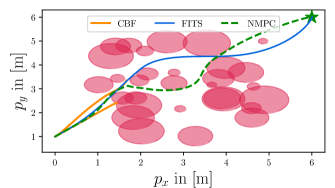
Figure 4: A two-dimensional navigation task. Obstacles are shown by red circles while the goal position is indicated by the green star.

References

- [1] A. D. Ames, X. Xu, J. W. Grizzle, and P. Tabuada, “Control barrier function based quadratic programs for safety critical systems,” Transactions on Automatic Control, vol. 62, no. 8, pp. 3861–3876, 2016.
- [2] K. Garg, J. Usevitch, J. Breeden, M. Black, D. Agrawal, H. Parwana, and D. Panagou, “Advances in the theory of control barrier functions: Addressing practical challenges in safe control synthesis for autonomous and robotic systems,” Annual Reviews in Control, vol. 57, p. 100945, 2024.
- [3] L. Grüne, J. Pannek, L. Grüne, and J. Pannek, Nonlinear model predictive control. Springer, 2017.
- [4] J. Breeden and D. Panagou, “Predictive control barrier functions for online safety critical control,” in Conference on Decision and Control (CDC). IEEE, 2022, pp. 924–931.
- [5] P. Jang, Inkyu, S. Hwang, J. Byun, and J. H. Kim, “Safe receding horizon motion planning with infinitesimal update interval,” in International Conference on Robotics and Automation. IEEE, 2024.
- [6] K. P. Wabersich and M. N. Zeilinger, “Predictive control barrier functions: Enhanced safety mechanisms for learning-based control,” Transactions on Automatic Control, vol. 68, no. 5, 2022.
- [7] J. Zeng, B. Zhang, and K. Sreenath, “Safety-critical model predictive control with discrete-time control barrier function,” in American Control Conference (ACC). IEEE, 2021, pp. 3882–3889.
- [8] M. Vahs, C. Pek, and J. Tumova, “Belief control barrier functions for risk-aware control,” IEEE Robotics and Automation Letters, 2023.
- [9] M. Vahs and J. Tumova, “Risk-aware control for robots with non-gaussian belief spaces,” in International Conference on Robotics and Automation (ICRA). IEEE, 2024.
- [10] M. Black, M. Jankovic, A. Sharma, and D. Panagou, “Future-focused control barrier functions for autonomous vehicle control,” in American Control Conference (ACC). IEEE, 2023, pp. 3324–3331.
- [11] T. Gurriet, M. Mote, A. D. Ames, and E. Feron, “An online approach to active set invariance,” in Conference on Decision and Control (CDC). IEEE, 2018, pp. 3592–3599.
- [12] Y. Chen, M. Jankovic, M. Santillo, and A. D. Ames, “Backup control barrier functions: Formulation and comparative study,” in Conference on Decision and Control (CDC). IEEE, 2021, pp. 6835–6841.
- [13] A. Wiltz, X. Tan, and D. V. Dimarogonas, “Construction of control barrier functions using predictions with finite horizon,” in Conference on Decision and Control (CDC). IEEE, 2023, pp. 2743–2749.
- [14] J. Zeng, Z. Li, and K. Sreenath, “Enhancing feasibility and safety of nonlinear model predictive control with discrete-time control barrier functions,” in Conference on Decision and Control (CDC). IEEE, 2021, pp. 6137–6144.
- [15] S. Gros, M. Zanon, R. Quirynen, A. Bemporad, and M. Diehl, “From linear to nonlinear mpc: bridging the gap via the real-time iteration,” International Journal of Control, vol. 93, no. 1, pp. 62–80, 2020.
- [16] A. Zanelli, “Inexact methods for nonlinear model predictive control: stability, applications, and software,” Ph.D. dissertation, Dissertation, Universität Freiburg, 2021, 2021.
- [17] L. Numerow, A. Zanelli, A. Carron, and M. N. Zeilinger, “Inherently robust suboptimal mpc for autonomous racing with anytime feasible sqp,” arXiv preprint arXiv:2401.02194, 2024.
- [18] T. Ohtsuka, “A continuation/gmres method for fast computation of nonlinear receding horizon control,” Automatica, vol. 40, no. 4, pp. 563–574, 2004.
- [19] C. Shen, B. Buckham, and Y. Shi, “Modified c/gmres algorithm for fast nonlinear model predictive tracking control of auvs,” IEEE transactions on control systems technology, vol. 25, no. 5, pp. 1896–1904, 2016.
- [20] P. Kidger, R. T. Q. Chen, and T. J. Lyons, “”hey, that’s not an ode”: Faster ode adjoints via seminorms.” International Conference on Machine Learning, 2021.
- [21] X. Xu, “Constrained control of input–output linearizable systems using control sharing barrier functions,” Automatica, vol. 87, 2018.
- [22] S. Boyd and L. Vandenberghe, Convex optimization. Cambridge university press, 2004.
- [23] J. Breeden, K. Garg, and D. Panagou, “Control barrier functions in sampled-data systems,” IEEE Control Systems Letters, vol. 6, pp. 367–372, 2021.
- [24] A. D. Ames, G. Notomista, Y. Wardi, and M. Egerstedt, “Integral control barrier functions for dynamically defined control laws,” IEEE control systems letters, vol. 5, no. 3, pp. 887–892, 2020.
- [25] Z. Yuan, A. W. Hall, S. Zhou, L. Brunke, M. Greeff, J. Panerati, and A. P. Schoellig, “Safe-control-gym: A unified benchmark suite for safe learning-based control and reinforcement learning in robotics,” IEEE Robotics and Automation Letters, vol. 7, no. 4, pp. 11 142–11 149, 2022.
- [26] J. Bradbury, R. Frostig, P. Hawkins, M. J. Johnson, C. Leary, D. Maclaurin, G. Necula, A. Paszke, J. VanderPlas, S. Wanderman-Milne, and Q. Zhang, “JAX: composable transformations of Python+NumPy programs,” missing, 2018. [Online]. Available: http://github.com/google/jax
- [27] G. Wu and K. Sreenath, “Safety-critical control of a planar quadrotor,” in American control conference (ACC). IEEE, 2016, pp. 2252–2258.