[table]capposition=top
Quantile Slice Sampling
Abstract
We propose and demonstrate an alternate, effective approach to simple slice sampling. Using the probability integral transform, we first generalize Neal’s shrinkage algorithm, standardizing the procedure to an automatic and universal starting point: the unit interval. This enables the introduction of approximate (pseudo-) targets through importance reweighting, a technique that has popularized elliptical slice sampling. Reasonably accurate pseudo-targets can boost sampler efficiency by requiring fewer rejections and by reducing target skewness. This strategy is effective when a natural, possibly crude, approximation to the target exists. Alternatively, obtaining a marginal pseudo-target from initial samples provides an intuitive and automatic tuning procedure. We consider two metrics for evaluating the quality of approximation; each can be used as a criterion to find an optimal pseudo-target or as an interpretable diagnostic. We examine performance of the proposed sampler relative to other popular, easily implemented MCMC samplers on standard targets in isolation, and as steps within a Gibbs sampler in a Bayesian modeling context. We extend the transformation method to multivariate slice samplers and demonstrate with a constrained state-space model for which a readily available forward-backward algorithm provides the target approximation.
Keywords: Markov chain Monte Carlo, Gibbs sampling, Hybrid slice sampling, Independence Metropolis-Hastings, Transformation, Bayesian modeling
1 Introduction
Slice sampling (Swendsen and Wang, 1987; Edwards and Sokal, 1988; Besag and Green, 1993; Neal, 2003) offers a simple and attractive option among the wide array of Markov chain Monte Carlo (MCMC) techniques (Higdon, 1998; Damlen et al., 1999). The approach decomposes, into manageable steps, the task of drawing from a distribution that may be difficult to sample directly. Consider a random variable with density proportional to . Suppose we can factor into component densities, and that we can sample from the distribution having density . Augmenting with a latent auxiliary variable and specifying the joint density of and to be proportional to (where returns 1 for true statements and 0 otherwise), we recover a marginal density of proportional to and a pair of manageable full conditional distributions. Given , is uniformly distributed on the interval . Given , has density with support restricted to , commonly known as the slice region. This augmentation admits convenient Gibbs sampling in what Roberts and Rosenthal (1999) call the simple slice sampler. The closely related uniform simple slice sampler draws uniformly on and uniformly over the slice region .
Despite their excellent theoretical properties (Roberts and Rosenthal, 1999; Mira and Tierney, 2002; Planas and Rossi, 2018), simple slice samplers lag in popularity behind Metropolis-Hastings samplers. Reluctance to adopt slice samplers may stem from the following complications. The slice region in the second full conditional above is specific to the target density. If this region can be found analytically, sampling over requires a custom solution. If is not known, as is common in statistical applications, general hybrid strategies exist to embed a Markov transition kernel in the second full conditional update (of to obtain a valid draw on (Roberts and Rosenthal, 1997; Rudolf and Ullrich, 2018; Łatuszyński and Rudolf, 2024; Power et al., 2024). A general class of widely used hybrid techniques were proposed by Neal (2003). Many hybrid samplers require multiple evaluations of the target density and some require tuning. Finally, the performance of slice sampling with respect to autodependence in the chain is sensitive to the shape of (Planas and Rossi, 2018).
Recent innovations that address the above complications in the context of elliptical slice sampling (ELSlice; Murray et al., 2010) have prompted a surge of interest in slice sampling; these include Nishihara et al. (2014); Tibbits et al. (2014); Cabezas and Nemeth (2023), among others. We observe that ideas related to these innovations reveal a natural and appealing environment for techniques of Neal (2003), uncovering a framework that extends their applicability.
In this article, we propose a reformulation of the simple slice sampler, using the probability integral transform to alleviate the above bottlenecks in its hybrid implementation. This is accomplished by i) transforming to an equivalent target more amenable to slice sampling, ii) standardizing the hybrid step’s search for the slice region, and iii) replacing the various user inputs with a single input: an approximate target density.
The approximate target does not replace the target but acts similarly to a proposal distribution in a Metropolis-Hastings sampler. Like a proposal, the approximate target is stochastically corrected by an MCMC transition kernel. Indeed, our sampler can be thought of as a slice-sampling analogue of the independence Metropolis-Hastings algorithm (IMH; Liu, 1996). While high-fidelity approximations to the target yield the best performance, our focus is not on searching for an optimal approximation. Rather, we rely on the robust mechanics of hybrid slice sampling to correct rough approximations that are easy to specify. The result is a streamlined approach to slice sampling that can yield excellent performance.

The combined effect of introducing an approximate target and transforming, in a method we call quantile slice sampling, is visually illustrated in Figure 1. When a reasonably good approximate target can be found, the method replaces the problem of uniformly slice sampling the original target density in the left panel with that of uniformly slice sampling the density in the right panel. Both employ the shrinkage procedure of Neal (2003) a hybrid step that adaptively shrinks an initial interval by rejecting proposed draws that lie outside the slice region. In the original setting, the initial interval is an unknown subset of the support of , and it is respecified at each iteration. In contrast, the initial interval is automatic and comprehensive under the proposed transformation using the distribution function of the approximate target. The new target density flattens, approaching uniform as approximation fidelity increases, effectively expanding the slice region. In both panels of Figure 1, latent variable is drawn at the same height relative to the target evaluation at the previous point. With the chosen initial interval, the original sampler (left) has a narrow slice region (thick line on the horizontal axis) and is expected to reject at least one proposal for before finding the slice region. In contrast, the transformed sampler (right) is very likely to accept the first proposal because the slice region fills most of the initial interval.
This article proposes and demonstrates an alternate, effective approach to simple slice sampling with the shrinkage algorithms of Neal (2003). Using the probability integral transform, we generalize the shrinkage procedure in a natural and intuitive setting that reveals more general applicability in Section 2. This extension facilitates the introduction in Section 3 of an approximate target with importance reweighting, previously referenced in connection to IMH by Mira and Tierney (2002) and later introduced by Nishihara et al. (2014) to extend ELSlice to cases beyond those using a Gaussian prior. Quantile slice sampling uses the transformation with well-chosen approximate targets to potentially reduce both the number of target evaluations and autocorrelation. We examine approaches to specifying the approximate target in Section 4, where the transformation enables evaluation of approximation quality. Section 5 compares empirical performance of the proposed quantile slice and other samplers on standard univariate targets and within a Bayesian modeling scenario. Section 6 extends transformation and approximate targets to Neal’s (2003) shrinkage procedure on hyperrectangles for multivariate sampling. It is then applied in Section 7 to facilitate posterior sampling in a high-dimensional setting for which traditional slice sampling performs poorly. We conclude with discussion in Section 8. The appendix includes proofs to propositions and additional details to supplement several sections.
2 Transformation extends Neal’s shrinkage procedure
One key contribution of Neal (2003) is a hybrid step named the shrinkage procedure that adaptively shrinks an interval to find the slice region. The procedure, given in Figure 5 of Neal (2003), has an important role in recent innovations such as elliptical (Murray et al., 2010), factor (Tibbits et al., 2014), and latent (Li and Walker, 2023) slice sampling. Here, we overcome two limitations of the shrinkage procedure with a transformation that i) extends its use to simple slice samplers used in Section 3, and ii) proves useful for characterizing approximation quality in Section 4. A generalized shrinkage procedure also results as a byproduct.
The primary challenge to slice sampling with the shrinkage procedure is that bounds on the slice region are generally unknown. Thus, selecting the initial interval requires care. Starting too narrow can result in slow exploration, or even a reducible Markov chain if the target has multiple modes separated by regions having density equal to 0 (Mira and Roberts, 2003). Neal (2003) introduces two procedures (called “stepping out” and “doubling”) for initializing the interval prior to shrinking. Both require tuning or additional checks. Li and Walker (2023) address the initialization problem with stochastically adaptive intervals. If the target distribution has bounded support, one option is to initialize the interval to match the bounds. While this avoids the initial search, several shrinkage steps may increase runtime if the target density concentrates mass in a relatively small interval.
We bypass the problem of selecting an initial interval with a transformation that gives automatic and universal bounds. Consider a random variable with target distribution and density , factored into and density from which we can readily sample. The simple slice sampler is the natural candidate in this scenario. We can trivially return to the uniform simple case by writing the unnormalized target as , but this does not bound the support. Alternatively, we can we can return to the uniform simple case and bound the support in the following way.
Let denote the (continuous) cumulative distribution function (CDF) corresponding to with inverse-CDF for . Consider the transformation . Straightforward application of the probability integral transform yields an equivalent target
| (1) |
where denotes the uniform density on the interval . We can now apply a uniform simple slice sampler with the standard shrinkage procedure. Resulting Monte Carlo samples can be transformed back via . Samples from a converged chain in thus have stationary distribution . Note that the support of is always confined to the unit interval, regardless of the support for , admitting an automatic and universal initial interval for the shrinkage procedure.
The original shrinkage procedure assumes a uniform full conditional over the slice region. However, the argument above reveals that the shrinkage procedure extends beyond the uniform simple case to any simple slice sampler for which the factorization of target includes a density with corresponding (and computable) CDF and inverse-CDF. Shrinking uniformly over the slice region for equivalently shrinks on the quantiles of . Indeed, quantile functions are commonly used to produce draws from truncated distributions.
2.1 Generalized shrinkage procedure
The above transformation leads to another observation: the shrinkage procedure works generally as a transition kernel with adaptive rejection for any continuous distribution. To sample from a distribution supported on but restricted to a given set , one can construct a Markov chain that draws candidates from restricted to an interval (initially ) that shrinks around the previous value until a sample within is found. A single update of this procedure is outlined in Algorithm 1.
To implement an MCMC sampler, start the chain at and iteratively apply Algorithm 1 with and , which outputs . The correctness of the algorithm is established in Proposition 1; a proof is given in Section A1 of the appendix.
Proposition 1
A Markov chain using the procedure outlined in Algorithm 1 with continuous has stationary distribution with support restricted to .
This adaptive rejection sampler is useful for restricting the support of a distribution to some subset with (that is, under ) that is not known analytically, but for which can be tested. This is the problem motivating hybrid slice sampling. Algorithm 1 can also be embedded within a Gibbs sampler. The algorithm performs best if is an interval, and can perform poorly if consists of subintervals separated by an interval with high probability under .
3 A quantile slice sampler
The transformation in Section 2 simplifies working with the shrinkage procedure and extends its use to simple slice samplers (that is, beyond uniform simple). This enables introduction in Section 3.1 of an approximate target to improve sampler efficiency, a strategy that has proven useful for elliptical slice sampling. The result is a quantile slice sampler that can be viewed as a slice-sampling analogue of independence Metropolis-Hastings (IMH). We discuss the connection with IMH in Section 3.2.
3.1 Approximate targets
If there is substantial disagreement between the target and component densities, a uniform simple slice sampler applied to (1) will be inefficient, often requiring several shrinkage steps. To improve efficiency, we can employ what Li et al. (2020) call a pseudo-prior. Suppose that density provides an approximation to on the same (or extended) support, and that we can evaluate its inverse CDF, , for . Following Nishihara et al. (2014), Fagan et al. (2016), Li et al. (2020), and Mira and Tierney (2002), we rewrite the unnormalized target density
| (2) | ||||
where the importance ratio takes the place of the “likelihood” and assumes the role of the “pseudo-prior.” Because we use it to approximate the target, we prefer to call the pseudo-target density. Note that the factorization , used for intuition and to connect to Section 2, is not necessary; in (2) could be equivalently expressed as for any .
Quantile slice sampling proceeds as follows. Given unnormalized target density and user-specified pseudo-target density with accompanying CDF and inverse CDF , transform to . Then, apply uniform simple slice sampling with the shrinkage procedure to
| (3) |
and back transform . Samples from a converged chain have stationary distribution with density . The procedure for a single update is outlined in Algorithm 2. In practice, densities are evaluated on the log scale. An equivalent procedure employs a simple slice sampler without transformation by drawing followed by a draw for using Algorithm 1 with , , and . Although this alternate view is more concise, its practical implementation is generally no more efficient than Algorithm 2, which we find instructive. Furthermore, retaining samples is useful for evaluating pseudo-target quality. Note that a different pseudo-target can be chosen at each iteration of MCMC. This is useful if the target full conditional changes with the state in a Gibbs sampler.
The quality of the approximation to affects the efficiency of the algorithm in several ways. Well-chosen approximations make the transformed target more concave and flat, enlarging the slice region relative to the initial interval and leading to earlier acceptance of proposed draws (as in Figure 1). If the transformed target is less skewed than the original target, the MCMC chain will also exhibit less autocorrelation (Planas and Rossi, 2018). A perfect approximation reduces the problem to slice sampling a uniform distribution, wherein the first draw is always accepted. Poorly chosen approximations may increase the kurtosis of relative to the original target, decreasing efficiency. If the target has significant probability mass in regions of the support with low density in the pseudo-target, numerical instabilities involving floating point precision may arise (for example, CDF evaluations round to 1 for all inputs beyond a certain limit). We discuss strategies for selecting the pseudo-target in Section 4.
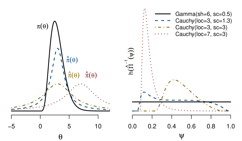
Figure 2 illustrates the effect of transformation under different pseudo-targets. The solid density on the left panel is the target (in this case, a gamma distribution) overlaid with three approximating location-scale Cauchy pseudo-targets. Aside from mismatched support, the pseudo-target with location 3 and scale 1.3 approximates the target well; the pseudo-target with location 3 and scale 3 inflates the scale; and the pseudo-target with location 7 and scale 3 exhibits both inflated scale and location bias. The right panel depicts the densities to be slice sampled upon transformation. In every case, the shrinking interval is initialized at . In most cases the sampler using the well-calibrated pseudo-target will require fewer than two shrinking steps, and often accept the first proposal.
Using a pseudo-target with heavier tails than the target effectively truncates the ends of the transformed target, slightly increasing the rejection rate (in this case, to approximately 0.67 rejections per iteration on average, compared with approximately 0.33 rejections per iteration for a comparable normal pseudo-target). We consider this a worthwhile trade-off to avoid convergence problems (Mira and Tierney, 2002) and floating point errors that can arise when a pseudo-target’s tails are lighter than those of the target. The sampler using a pseudo-target with inflated variance will often require a few shrinking steps, and in this case the number of required target evaluations is comparable to that of using a combination of stepping-out and shrinking steps from Neal’s (2003) workflow. The sampler using the pseudo-target with inflated variance and substantial location bias is less efficient, requiring more shrinking steps and yielding a chain with higher autocorrelation (still below 0.4). We consider ways to evaluate pseudo-target quality in Section 4.
3.2 Relation to independence Metropolis-Hastings
Pseudo-targets appear in IMH samplers as proposal distributions. Mira and Tierney (2002) compare the transition operators of IMH and slice sampling. Assuming the target , they specify a simple slice sampler that draws directly from truncated (that is, no hybrid extension), and an IMH sampler that draws proposals from and evaluates . If we introduce pseudo-target , both samplers retain their original structures, substituting with and with from (2). The IMH sampler proposes from and evaluates . Mira and Tierney (2002) prove (their Theorem 3) that for any IMH sampler with proposal , the corresponding slice sampler achieves “smaller asymptotic variance of sample path averages (on a sweep by sweep basis).” Note that the shrinkage procedure is not used in this comparison, which assumes that a draw on the slice region can be immediately obtained. Łatuszyński and Rudolf (2024) and Power et al. (2024) consider the effect of adding hybrid steps on convergence.
To build intuition for Mira and Tierney’s (2002) result, consider the following. The probability that IMH accepts a candidate drawn from is the minimum of 1 and , which is equivalent to accepting the candidate if a variable drawn uniformly on is less than . The slice sampler accepts initial candidate if with intermediate value drawn uniformly on . The two algorithms differ in that rejection in IMH leads to setting , whereas the slice sampler guarantees acceptance, either by sampling directly on the slice region or by repeatedly drawing from until a draw within the slice region is found.
Framing the quantile slice sampler in terms of IMH also suggests one way to evaluate the quality of approximation by the pseudo-target. The probability of making a transition in IMH from point is equal to
| (4) |
where , is defined in (2), and is the support of . Equation 4 can be interpreted as the expected probability of accepting a proposal drawn from when the current state is . A successful pseudo-target yields close to a constant function and near 1 across . Finally, if the target distribution is known, we can average across starting values from the stationary target
| (5) | ||||
This measure of pseudo-target fitness takes on values in the unit interval, with 1 resulting from perfect agreement between and , that is, a sampler that accepts every proposal.
4 Selecting a pseudo-target
The performance of samplers employing pseudo-targets hinges on the quality of approximation. Pairing pseudo-targets with slice sampling and the shrinkage procedure offers a degree of robustness. That is, transformation to a reasonable pseudo-target yields a reasonably performant sampler. Aided by the transformation underlying (3), we seek to quantify pseudo-target fidelity, leading to methods for initial or intermediate selection of approximate targets, as well as diagnostic metrics for post-sampling evaluation.
General strategies for target approximation include Laplace approximations, parallel augmented Gibbs samplers (Nishihara et al., 2014), and optimizing distance metrics for distributions, such as Kullback Leibler divergence (Cabezas and Nemeth, 2023). For example, one could set the location and scale of the pseudo-target to match those of a Laplace approximation to the target density. If an approximation to the moments of the target distribution exists, this could also be used similarly to obtain an easy and inexpensive “moment matching” pseudo-target.
We propose selecting within a class of pseudo-target distribution families (usually Student-) and offer two optimization criteria in Sections 4.1 and 4.2. The first connects to the IMH acceptance probability. The second is more intuitive, less computationally expensive, and works well in practice.
4.1 Quantifying pseudo-target fidelity
We aim to measure approximation quality through its effect on two aspects of algorithm performance: i) autodependence in the Markov chain and ii) cost of repeated target evaluations in search of the slice region. Simple slice samplers with known slice regions are concerned only with the first aspect. Planas and Rossi (2018) observed that the interleaving property of two-stage Gibbs samplers (Liu et al., 1994) connects target skewness and chain autocorrelation in simple slice samplers. Specifically, the covariance between and is equal to , where the variance is taken with respect to the joint marginal distribution of and the intermediate auxiliary uniform variable defining the slice, . This result suggests that autocorrelation from slice samplers is reduced for target distributions with low skewness, and is equal to zero for centrally symmetric targets (Planas and Rossi, 2018). Thus, transformations that reduce skewness are desirable.
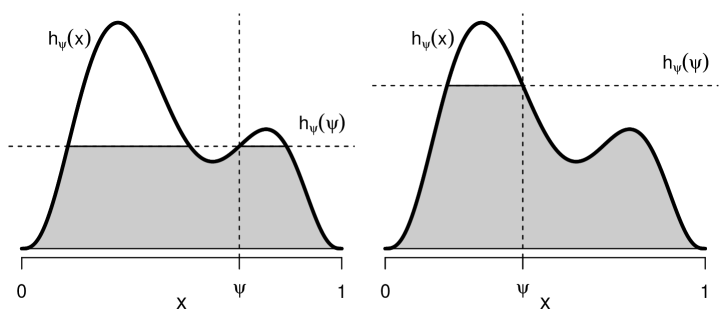
Repeated target evaluation in search of the slice region is of more practical than theoretical concern. Transformation to the distribution function of a pseudo-target clarifies the problem. The procedure of drawing uniformly from an interval suggests that the number of rejections is minimized when the total length of the slice region is maximized. Let denote the unnormalized, transformed target density from (3) supported on , and let . We assume that , as transformations yielding vertical asymptotes lead to numerical instability. Further denote as the total length of the slice region as a function of the auxiliary latent variable drawn uniformly on . Calculating total length for may include aggregating lengths of disconnected components of the slice region. The expected total slice length, with respect to the marginal (stationary) distribution of , is given as
| (6) | ||||
where is interpretable as the normalized area of the region , as depicted in Figure 3 for two values of with generic . Note that and that is averaged with respect to a uniform distribution on rather than the target distribution.
The transformation reveals two important connections with IMH in Section 3.2. The following proposition establishes equivalence of the two evaluation criteria described thus far. A proof is given in Section A2 of the appendix.
Proposition 2
Let and represent absolutely continuous target and pseudo-target densities with respective supports and distribution functions and . Further let , for some normalizing constant , on and 0 otherwise, and . Assume for all . Finally, let represent a draw from , with corresponding . Consider an IMH sampler using target with proposal , a simple slice sampler using target , and a uniform simple slice sampler using target . Then the following three quantities are equal to one another:
-
1.
Expected acceptance probability of IMH proposal,
from (4). -
2.
Expected probability of the slice region under computed as
for . -
3.
Expected total slice width with .
Another consideration is related to the iterative shrinking behavior in the standard shrinking procedure and in 1. Upon rejection of a candidate point, shrinking the boundary to the most recent point drawn introduces additional autocorrelation as an artifact if the slice region is composed of disconnected subintervals. This can occur if is multimodal.
4.2 An alternate objective function
Now consider scaling by so that is enclosed within the unit square. We substitute the problem of finding a pseudo-target and corresponding that maximizes (6) with the significantly easier problem of maximizing the area under the curve. We denote the alternate objective as AUC, formally defined as , which can take on values in .
Unfortunately, AUC and (6) do not have a one-to-one correspondence. It is possible to shift mass in ways that increase AUC while decreasing (6). However, the global maximum is achieved for both only when is a constant function. In our experience, searches for pseudo-targets aimed at maximizing AUC typically push toward distributions approaching uniform, and therefore high values of (6). Furthermore, cases in which AUC and (6) disagree can be easily detected. We have also considered modifications of AUC, including penalties for skewness and for multiple local modes. Empirical evidence suggests that the marginal gains these two penalties provide do not justify the complexity they introduce.
In practice, we recommend maximizing AUC within a class of candidate pseudo-target distributions. This can be done prior to sampling by numerical integration of , optimizing over the parameters of the chosen family of pseudo-targets. Alternatively, AUC can be approximated with a histogram using samples transformed to under a proposed pseudo-target. Both approaches are used in Section 5.
Samples of can further be used for interpretable sampler diagnostics and tuning. The shape of the histogram indicates which adjustments to the pseudo-target can improve efficiency. For example, off-center (from 0.5) histograms indicate a location bias. Narrow histograms indicate the pseudo-target is too diffuse, while U-shaped histograms indicate the pseudo-target is too narrow and/or has insufficient tail mass.
5 Illustrations and sampler performance
This section examines performance of the quantile slice sampler (QSlice) relative to other popular, easily implemented MCMC samplers. We begin with a simulation study comparing sampler performance on three standard targets in Section 5.1. In Section 5.2, we illustrate use of QSlice in a Bayesian modeling context, as a step within a Gibbs sampler.
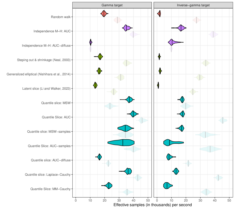
In both experiments, competing algorithms include random-walk Metropolis (RWM), independence Metropolis-Hastings (IMH), a uniform simple slice sampler using Neal’s (2003) shrinkage procedure preceded by the stepping-out procedure (step & shrink), the generalized elliptical slice sampler (Nishihara et al., 2014), and the latent slice sampler (Li and Walker, 2023). Performance is evaluated using effective samples (Plummer et al., 2006) per CPU second (ESpS). Additional details are provided in Section A3 of the appendix. Implementations of all slice samplers and IMH are available in the R package qslice (Heiner et al., 2024).
5.1 Simulating standard targets
This experiment tests all samplers in isolation on three representative target families: standard normal, gamma (shape 2.5 and scale 1), and inverse gamma (shape 2 and scale 1). The gamma target represents distributions with skew and light tails, and the inverse-gamma target represents extreme skew and heavy tails. Competing samplers were tuned for performance in ESpS using preliminary runs.
Quantile slice samplers all use Student- pseudo-targets with left truncation at 0 for targets with nonnegative support. Despite some mismatch on the lower quantiles, truncated distributions adequately capture skewness in the gamma and inverse-gamma targets. Polynomial tails also avoid numerical issues at little computational cost. For these reasons, we generally recommend distributions as the default family for pseudo-targets.
We employed four strategies to further specify Student- pseudo-targets (location, scale, and degrees of freedom in ): i) numerically maximize either mean slice width (MSW; see section 4.1) or area under the transformed density curve (AUC; see Section 4.2); ii) maximize histogram-estimated MSW or AUC using 1,000 independent samples from the target; iii) Laplace approximation with a Cauchy pseudo-target; and iv) crude “moment” (location and scale) matching between target and a Cauchy pseudo-target (MM). We also included a pseudo-target misspecification scenario in which the scale of the pseudo-target from the AUC method was inflated by a factor of 4 (AUC–diffuse). AUC-based pseudo-targets also served as proposal distributions in IMH samplers.
Figure 4 summarizes ESpS from 100 independent MCMC chains using the tuned algorithms. We first observe that methods employing pseudo-targets can react better to skewness and heavy tails than RWM and existing slice methods. They are, however, sensitive to the quality of approximation; IMH with a high-quality approximation performs well, but deteriorates to worst performance with poor approximation (AUC–diffuse) when using normal and gamma targets.
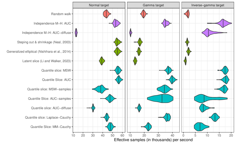
With a univariate, unimodal target and good approximation, the IMH accept/reject decision that always moves on after two target evaluations can be more efficient than QSlice. However, guaranteed moves within the slice region mitigate the effects of poor approximation. Although high-fidelity approximations will always yield optimal performance, QSlice can yield strong performance with mediocre approximations (for example, MM–Cauchy). This can be useful in Gibbs samplers where approximating the target full conditional at each iteration is expensive, but crude approximations are readily available. QSlice offers some robustness to pseudo-target misspecification, which can render IMH unusable.
The AUC alternative for pseudo-target specification appears to yield superior performance to the computationally expensive MSW method. Despite introducing variability, using initial samples from the target to specify a pseudo-target performs well and provides an easy, interpretable tuning procedure.
5.2 Bayesian modeling: hyper-g prior
Our second illustration uses Zellner’s (1986) prior for Bayesian linear regression. In this setting, we observe performance of an algorithm embedded within a Gibbs sampler and test sampler diagnostics. We also compare two strategies for pseudo-target specification: approximating the full conditional and marginal posterior distributions.
The model is given as
| (7) | ||||
where is a vector of (centered/scaled) responses, is a full-rank by matrix of (centered/scaled) covariates, is a vector of regression coefficients, scalar is the error variance, and scalar shrinks toward . The model is completed with an inverse-gamma prior for and the hyper- prior proposed by Liang et al. (2008), which we adopt after restricting .
We use the Motor Trend road test (mtcars) data from the R datasets package (Henderson and Velleman, 1981; R Core Team, 2024) with observations of miles per gallon (mpg) as the response and all remaining variables as covariates. Our prior specification uses , following Liang et al. (2008), and inverse gamma for with shape and scale .
To sample from the joint posterior distribution of , our Gibbs sampler cycles through conjugate updates of and , and employs one of the competing algorithms to sample from the full conditional of . Each MCMC algorithm begins with a burn-in phase of 10,000 iterations using step & shrink for . This is followed by an adaptive tuning phase, specific to each sampler for . After tuning, algorithm settings are fixed and the sampler proceeds for 50,000 timed iterations. We timed 100 independent chains for each sampler type. Additional details are given in Section A4 of the appendix.
We employ two strategies for pseudo-target specification, used with each of the IMH and the generalized elliptical and quantile slice samplers. The first strategy constructs the pseudo-target from 2,000 of the burn-in samples of by finding a Student- distribution that minimizes the (histogram-based) AUC, thus relying on the marginal posterior distribution of for an approximation to the full conditional. This approach is sensitive to dependence of on and in the posterior; high dependence yields a full conditional that concentrates mass on a smaller subset of values than the marginal density. We check for this by monitoring the number of shrinking steps needed to accept a draw at each iteration; for a summary, see Table 1. With QSlice, the AUC–samples approach averages rejections, indicating a relatively efficient pseudo-target. Another diagnostic uses the sampled . The left panel of Figure 5 gives a histogram of these samples for a typical run. The are reasonably close to uniformly distributed, indicating that the pseudo-target is well calibrated to the marginal posterior.
| Sampler | Pseudo-target | Evaluations per iteration | |
|---|---|---|---|
| method | |||
| Random walk | n/a | 2 (fixed) | 2 (fixed) |
| Independence M-H | all | 2 (fixed) | 2 (fixed) |
| Stepping out & shrinkage | n/a | ||
| Latent slice | n/a | ||
| Generalized elliptical | AUC–samples | ||
| Laplace analytic | |||
| Laplace analytic (wide) | |||
| Quantile slice | AUC–samples | ||
| Laplace analytic | |||
| Laplace analytic (wide) | |||
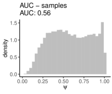
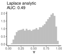
Our second strategy for specifying the pseudo-target is to approximate the full conditional. In the case of the hyper- prior, the full conditional can be closely approximated with an inverse-gamma distribution, suggesting this family for a pseudo-target. Unfortunately, extremely low density values near the origin make inverse gamma a numerically unstable choice for pseudo-targets generally. We opt for the default choice of truncated Student-, in this case relying on an analytical Laplace approximation (see Section A4 of the appendix for details). Although numerical Laplace approximation is feasible, we find it challenging to make reliable and competitive, as it requires respecification at each MCMC iteration. One could alternatively set the location and scale of the pseudo-target to “match” the approximating inverse gamma.
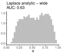
The histogram of in the center panel of Figure 5 reveals that substantial probability mass in the full conditional lies outside the bulk of the Laplace-approximated pseudo-target. We therefore increase (tune) the scale of the pseudo-target by 50%, which we refer to as the Laplace–wide pseudo-target (right panel of Figure 5). This results in a distribution closer to uniform and higher sample AUC values, which also serve as summary diagnostic indicators of pseudo-target fitness.
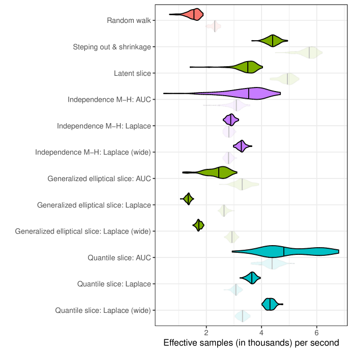
Timing results are summarized with violin plots in Figure 6. Because it is common to transform variables with restricted support, we also report timing results for each of the samplers applied to sampling (light shading). The Laplace–wide scale inflation factor is 20% when sampling . Transformation reduces skew in the target and substantially improves performance of several samplers.
The step & shrink algorithm sampling outperforms QSlice tuned with initial samples, on average. However, Table 1 reveals that step & shrink also averages more than twice as many target evaluations as QSlice. Repeated target evaluations can degrade ESpS in scenarios with computationally expensive targets. Despite volatility from dependence on a preliminary MCMC sample, Qslice with AUC–samples yields excellent performance, even within a Gibbs sampler.
6 Multivariate sampling
The univariate quantile slice sampler described thus far provides an appealing alternative to standard sampling methods when a suitable pseudo-target can be found. Pseudo-targets also help mitigate challenges to sampling in multiple dimensions, where for example, the stepping-out procedure is not available and IMH suffers from high rejection rates. While we recommend the generalized elliptical slice sampler (Nishihara et al., 2014) for approximately Gaussian (or multivariate ) targets with unrestricted support, a multivariate extension of the quantile slice sampler would be well-suited for cases with nonstandard or restricted support and where a natural approximation to the target exists. Such targets arise when models can be approximated by simpler versions.
Neal (2003) explores multivariate slice-sampling schemes that use a single latent variable, avoiding augmentation in each dimension. Most notably, the shrinkage procedure trivially generalizes to multiple dimensions. An algorithm for a rejection sampler that generalizes the shrinking interval with shrinking along each axis of a hyperrectangle is given as Figure 8 in Neal (2003).
6.1 Uncorrelated targets
The importance reweighting expression in (2) applies readily for random vectors . However, transformation to a vector that is uniformly distributed on requires care. If elements of are approximately independent in the target distribution (or undergo a decorrelating rotation; Tibbits et al., 2014), then a pseudo-target built from independent components may suffice. That is, we can use and transform to with univariate CDFs corresponding to the densities . The sampler proceeds with the standard multivariate shrinkage procedure applied to with one modification: the hypperrectangle is always initialized as the -dimensional unit hypercube.
Natural transformations to approximately independent targets exist in some common cases. For example, if is compositional (that is, nonnegative entries that sum to one) and approximately satisfies complete neutrality, we can exploit the stick-breaking representation of the generalized Dirichlet distribution of Connor and Mosimann (1969). This representation uses mutually independent beta-distributed variables to construct .
6.2 Approximations from chained conditional distributions
Chained conditional distributions provide another avenue for mapping multivariate random vectors to .
If a decomposition of is readily available, we can transform to using the chained sequence of conditional CDFs, that is, .
Conveniently, the Jacobian of this transformation has determinant equal to
, which cancels in the numerator of (2), again admitting a slice sampler with a multivariate shrinkage procedure applied to .
We use this construction in Section 7.
7 Illustration: non-Gaussian dynamic linear model
We demonstrate application of the multivariate quantile slice sampler in a scenario to which it is well suited. The objective is to sample conditional block updates of constrained time-varying parameters (TVPs) within a dynamic linear model (DLM). We compare algorithm performance among several alternatives.
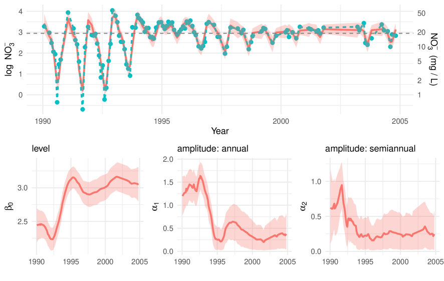
We apply DLMs to time series of nitrate (NO) concentrations in a stream in France, collected at approximately monthly intervals (Naïades, 2018). Nitrate pollution in streams, typically attributed to agricultural activity, can cause harmful algal blooms in a process referred to as eutrophication (Le Moal et al., 2019). Monitoring both long-term trends and seasonality is helpful to management efforts (Abbott et al., 2018). The top panel of Figure 7 shows a time series for a stream that exhibits drift in both the level (that is, mean concentration) and the amplitude of an annual cycle. The plot indicates a target NO concentration of 19 mg/L, at which reductions of eutrophication may begin (Dodds et al., 1998; Perrot et al., 2014; Abbott et al., 2018).
7.1 Dynamic harmonic regression model
We fit a dynamic harmonic regression (DHR) model that combines harmonic regression with TVPs (Young et al., 1999; Mindham and Tych, 2019; West, 1995). DHR is traditionally parameterized using Fourier coefficients, conflating variability in the amplitudes and phases of the cycles and thus complicating prior elicitation. We model amplitudes and phases directly, which introduces constraints to the model and complicates MCMC.
Let represent the log-NO concentration at time , measured continuously in years, for observation index ; in this case, . The DHR model is given as
| (8) |
with time-indexed intercepts , amplitudes of the annual cycle with static phase , amplitudes of the semiannual cycle with static phase , and independent observation noise . The time-varying parameters are given initial distributions , , and , and evolve according to random walks with continuous-time adjustment
where the indicate truncation at 0 to enforce positivity constraints. The model is completed with uniform priors on and , and an inverse-gamma prior on with shape and scale . Implementation details are given in Section A5 of the appendix.
The lower panel of Figure 7 summarizes posterior inferences for the TVPs with evolving means and 90% credible intervals. Posterior distributions for the amplitude parameters press against the lower boundary of 0, which helps with identifiability of (8) since negative amplitude values shift the corresponding phases. Such behavior is sometimes observed in samples from the standard forward-filter and backward-sampling (FFBS; Carter and Kohn, 1994; Frühwirth-Schnatter, 1994) update for TVPs with no boundary constraints.
7.2 Pseudo-target
Despite nonidentifiability, FFBS is useful for posterior sampling if used as the basis of a pseudo-target for the full conditional distributions of , . Specifically, the algorithm exploits the Markovian prior and conditional independence to decompose the joint full conditional for into a chain of univariate densities
| (9) |
where is understood to mean all observations up to time index . The conditional distributions in (9) are Gaussian provided the initial distributions, state evolution distributions, and observation distributions for are linear and Gaussian.
We construct a joint pseudo-target for from a chain of univariate conditional densities, as in Section 6.2. The pseudo-target distributions are truncated Gaussian or Student- with location and scale parameters obtained from the corresponding distributions in (9). The transformation using the chain of conditional pseudo-target CDFs yields a one-to-one mapping from to on which we apply the multivariate slice sampler with shrinkage. The algorithm to update of , and other implementation details, are in Section A5 of the appendix.
7.3 Performance comparison
We compare the efficiency of the multivariate quantile slice (MQSlice) sampler to that of other candidate algorithms for the amplitude updates. We include generic multivariate samplers as well as a particle Gibbs sampler that is standard for non-Gaussian DLMs. We notably exclude the elliptical slice sampler, for which truncation is problematic, and gradient-assisted MCMC, which is not easily incorporated within the Gibbs sampler.
The first generic sampler is IMH with the FFBS-based pseudo-target described above as a proposal distribution, similar to the strategies discussed in Fearnhead (2011). We also compare against multivariate versions of two slice samplers: i) with the standard shrinkage procedure on a hyperrectangle with no pseudo-target and no transformation (MSlice; Neal, 2003), and ii) the latent slice sampler of Li and Walker (2023). Both slice samplers restrict the hyperrectangle to exclude negative amplitudes.
We add two comparisons that are specific to DLMs. First is the FFBS algorithm, which is not a true competitor to the other samplers because it does not address truncation and samples a nonidentified model. FFBS is the only algorithm that updates as a single block, and it is included as a benchmark. The second specialized algorithm is a particle MCMC sampler that uses conditional sequential Monte Carlo within a Gibbs framework. Our implementation specifically uses the bootstrap filter with a backward-sampling step (Chopin and Papaspiliopoulos, 2020, Ch. 16).
The MQSlice and IMH samplers require initial specification of the pseudo-target. The MSlice, latent, and particle samplers were each tuned using pilot runs. Timing runs at selected settings consisted of two chains, each with 2,000 burn-in iterations followed by 20,000 iterations (both stages were increased five-fold for the MSlice and latent runs).
Table 2 reports results from the full experiment, which consisted of 50 replicate timing runs for each algorithm, following the protocol outlined in Section A3 of the appendix. Reported effective sample sizes were aggregated from both chains and summarized (mean, minimum) across the parameters in , and were computed using the coda R package (Plummer et al., 2006). We also report summaries of the potential scale reduction factors (PSRF; Gelman and Rubin, 1992) as a measure of convergence, and the number of target evaluations per iteration.
| Sampler | Settings | PSRF | ESpS | ESpS | Target |
|---|---|---|---|---|---|
| (mean) | (minimum) | evaluations | |||
| IMH | pseudo: Gaussian | (fixed) | |||
| pseudo: | (fixed) | ||||
| MSlice | |||||
| Latent | |||||
| MQSlice | pseudo: Gaussian | ||||
| pseudo: | |||||
| Particle | particles | n/a | |||
| FFBS | n/a |
MQSlice is the only high-performing slice sampler in this experiment, achieving strong ESpS and stable diagnostics when using Gaussian pseudo-targets, and is still the preferred slice sampler when using a more robust Student- pseudo-target. PSRF results indicate that the general slice samplers struggle with parameter vectors of length . The number of target evaluations reveals that these samplers shrink so far at each iteration that the space is not efficiently explored, though the chains do trace the correct posterior distribution (albeit with high autocorrelation) and yield a reasonable fit. Our results confirm that particle MCMC is particularly well suited to posterior sampling for non-Gaussian TVPs. The FFBS fit is not identifiable despite positive MCMC diagnostics.
High ESpS for IMH reveals that FFBS-based truncated Gaussian pseudo-targets approximate the joint full conditionals with excellent fidelity in this example. IMH outperforms quantile slice sampling in mean ESpS, although IMH mixing performance is somewhat volatile. Performance of MQSlice and IMH is sensitive to the tails of high-dimensional pseudo-targets. While heavy tails protect from numerical instability under pseudo-target misspecification, they can become a liability in the multivariate setting. It is well known that as proposal distributions drift from the target, IMH degrades to the point of rejecting most proposed moves. In our DHR example, MQSlice yields higher minimum ESpS and lower PSRF than does IMH when the pseudo-target is with 5 degrees of freedom. This advantage is less evident when (not shown).
This timing experiment employed custom implementations of each competing algorithm, written in R (in which several functions call precompiled C code). It is important to recognize that benchmarking results will vary by hardware, operating system, programming language, and implementation. For example, the MQSlice sampler written for DHR runs approximately 3-8 times faster than when implemented with a more general framework for pseudo-target specification in the qslice package (Heiner et al., 2024).
8 Discussion
This paper revisits slice sampling with the shrinkage procedure of Neal (2003), extending its applicability and in some cases substantially improving its performance. The probability integral transform allows shrinking from an automatic and universal starting point, the unit interval, and enables introduction of pseudo-targets, following Nishihara et al. (2014) and others. The resulting quantile slice sampler can be viewed as a slice-sampling analogue of independence Metropolis Hastings.
Pseudo-targets that reasonably approximate the target distribution can boost sampler efficiency in two ways: i) by requiring fewer rejections, and ii) by slice sampling a target with reduced skewness. This strategy is particularly effective when a natural, possibly crude, approximation to the target exists. If not, obtaining a marginal pseudo-target from initial samples provides an intuitive and automatic tuning procedure. We have introduced two metrics with which to evaluate the quality of approximation. The intuitive AUC metric can be used to find an optimal pseudo-target or as a diagnostic measure.
Our experiments have demonstrated that the stepping-out and shrinkage procedure of Neal (2003) is effective as a general sampler for univariate targets (with low skewness) for which evaluation is inexpensive. We have also found its performance to be insensitive to specification of the tuning parameter. Absent a natural candidate to approximate a univariate target, we recommend employing stepping-out and shrinkage during a burn-in phase and using the initial samples to specify a pseudo-target for use with a quantile slice sampler thereafter. This tuning procedure is effective provided that the marginal distribution is not overly diffuse relative to the target full conditional. The tuning step requires no repeated application and no analysis of the target.
Among slice samplers, we recommend generalized elliptical slice sampling (Nishihara et al., 2014) for multivariate targets with unrestricted support. As with other multivariate slice samplers, elliptical slice samplers introduce one latent variable. However, they shrink on only one dimension, and are generally far more efficient than samplers that shrink along each axis of a hyperrectangle. Development of strategies for transformations to targets amenable to elliptical slice sampling has garnered recent attention (Cabezas and Nemeth, 2023). As discussed in Section 6 and demonstrated in Section 7, multivariate quantile slice samplers can be used to leverage an available approximation to a complex or constrained target, possibly opening a viable slice-sampling alternative.
A primary limitation of quantile slice sampling is its sensitivity to the quality of target approximation. If one is concerned with optimal sampling performance, a high-fidelity pseudo-target is required. In cases where it is sufficient to find a viable sampler that requires little or no tuning, the quantile slice sampler is an attractive option. Nevertheless, badly misspecified pseudo-targets can result in numerical instability.
Quantile and latent slice sampling use what could be termed as assisted or informed shrinkage procedures. The concept of informed shrinkage could potentially give rise to other rejection-based samplers that outperform Metropolis-Hastings counterparts. Areas with potential for innovation may include shrinkage on gradient assisted pseudo-targets, targeted shrinkage, and sampling discrete variables with support too large to enumerate. Metropolis-Hastings proposals on large discrete spaces are often modest to avoid frequent rejection, resulting in slow exploration. In contrast, informed shrinkage procedures can potentially offer improved balance between local movement and target exploration.
Acknowledgements
The authors gratefully acknowledge helpful conversations with Godwin Osabutey.
SUPPLEMENTARY MATERIALS
- Appendix:
- Code:
-
(GitHub repository) https://github.com/mheiner/qslice_examples.
R scripts to recreate examples and results in the paper. Descriptions are given in the README files.
References
- Abbott et al. (2018) Abbott, B. W., Moatar, F., Gauthier, O., Fovet, O., Antoine, V., and Ragueneau, O. (2018), “Trends and seasonality of river nutrients in agricultural catchments: 18 years of weekly citizen science in France,” Science of the Total Environment, 624, 845–858.
- Besag and Green (1993) Besag, J. and Green, P. J. (1993), “Spatial Statistics and Bayesian Computation,” Journal of the Royal Statistical Society Series B: Statistical Methodology, 55, 25–37.
- Cabezas and Nemeth (2023) Cabezas, A. and Nemeth, C. (2023), “Transport Elliptical Slice Sampling,” in Ruiz, F., Dy, J., and van de Meent, J.-W. (editors), Proceedings of The 26th International Conference on Artificial Intelligence and Statistics, volume 206 of Proceedings of Machine Learning Research, PMLR, URL https://proceedings.mlr.press/v206/cabezas23a.html.
- Carter and Kohn (1994) Carter, C. K. and Kohn, R. (1994), “On Gibbs Sampling for State Space Models,” Biometrika, 81, 541–553.
- Chopin and Papaspiliopoulos (2020) Chopin, N. and Papaspiliopoulos, O. (2020), An Introduction to Sequential Monte Carlo, Springer Series in Statistics, Springer Nature Switzerland: Springer Cham, first edition, URL https://link.springer.com/book/10.1007/978-3-030-47845-2.
- Connor and Mosimann (1969) Connor, R. J. and Mosimann, J. E. (1969), “Concepts of Independence for Proportions with a Generalization of the Dirichlet Distribution,” Journal of the American Statistical Association, 64, 194–206.
- Damlen et al. (1999) Damlen, P., Wakefield, J., and Walker, S. (1999), “Gibbs sampling for Bayesian non-conjugate and hierarchical models by using auxiliary variables,” Journal of the Royal Statistical Society: Series B (Statistical Methodology), 61, 331–344.
- Dodds et al. (1998) Dodds, W. K., Jones, J. R., and Welch, E. B. (1998), “Suggested classification of stream trophic state: distributions of temperate stream types by chlorophyll, total nitrogen, and phosphorus,” Water Research, 32, 1455–1462.
- Edwards and Sokal (1988) Edwards, R. G. and Sokal, A. D. (1988), “Generalization of the Fortuin-Kasteleyn-Swendsen-Wang representation and Monte Carlo algorithm,” Physical Review D, 38, 2009.
- Fagan et al. (2016) Fagan, F., Bhandari, J., and Cunningham, J. P. (2016), “Elliptical Slice Sampling with Expectation Propagation,” in Proceedings of the Thirty-Second Conference on Uncertainty in Artificial Intelligence, Jersey City, New Jersey.
- Fearnhead (2011) Fearnhead, P. (2011), “MCMC for State-Space Models,” in Handbook of Markov Chain Monte Carlo, Boca Raton: Chapman & Hall/CRC.
- Frühwirth-Schnatter (1994) Frühwirth-Schnatter, S. (1994), “Data augmentation and dynamic linear models,” Journal of Time Series Analysis, 15, 183–202.
- Gelman and Rubin (1992) Gelman, A. and Rubin, D. B. (1992), “Inference from Iterative Simulation Using Multiple Sequences,” Statistical Science, 7, 457–472.
- Heiner et al. (2024) Heiner, M., Dahl, D. B., and Johnson, S. (2024), qslice: Implementations of Various Slice Samplers, URL https://CRAN.R-project.org/package=qslice. R package version 0.3.1.
- Henderson and Velleman (1981) Henderson, H. V. and Velleman, P. F. (1981), “Building Multiple Regression Models Interactively,” Biometrics, 391–411.
- Higdon (1998) Higdon, D. M. (1998), “Auxiliary Variable Methods for Markov Chain Monte Carlo with Applications,” Journal of the American Statistical Association, 93, 585–595.
- Le Moal et al. (2019) Le Moal, M., Gascuel-Odoux, C., Ménesguen, A., Souchon, Y., Étrillard, C., Levain, A., Moatar, F., Pannard, A., Souchu, P., and Lefebvre, A. (2019), “Eutrophication: A new wine in an old bottle?” Science of the Total Environment, 651, 1–11.
- Li et al. (2020) Li, S., Tso, G. K., and Li, J. (2020), “Parallel generalized elliptical slice sampling with adaptive regional pseudo-priors,” Journal of Statistical Computation and Simulation, 90, 2789–2813.
- Li and Walker (2023) Li, Y. and Walker, S. G. (2023), “A latent slice sampling algorithm,” Computational Statistics and Data Analysis, 179, 107652.
- Liang et al. (2008) Liang, F., Paulo, R., Molina, G., Clyde, M. A., and Berger, J. O. (2008), “Mixtures of Priors for Bayesian Variable Selection,” Journal of the American Statistical Association, 103, 410–423.
- Liu (1996) Liu, J. S. (1996), “Metropolized independent sampling with comparisons to rejection sampling and importance sampling,” Statistics and Computing, 6, 113–119.
- Liu et al. (1994) Liu, J. S., Wong, W. H., and Kong, A. (1994), “Covariance structure of the Gibbs sampler with applications to the comparisons of estimators and augmentation schemes,” Biometrika, 81, 27–40.
- Mindham and Tych (2019) Mindham, D. A. and Tych, W. (2019), “Dynamic harmonic regression and irregular sampling; avoiding pre-processing and minimising modelling assumptions,” Environmental modelling & software, 121, 104503.
- Mira and Roberts (2003) Mira, A. and Roberts, G. O. (2003), “[Slice sampling]: Discussion,” The Annals of Statistics, 31, 748–753.
- Mira and Tierney (2002) Mira, A. and Tierney, L. (2002), “Efficiency and Convergence Properties of Slice Samplers,” Scandinavian Journal of Statistics, 29, 1–12.
- Murray et al. (2010) Murray, I., Adams, R., and MacKay, D. (2010), “Elliptical slice sampling,” in Proceedings of the Thirteenth International Conference on Artificial Intelligence and Statistics, JMLR Workshop and Conference Proceedings.
- Naïades (2018) Naïades (2018), “Physicochemistry data for Whole France,” Data retrieved November 2018, URL http://www.naiades.eaufrance.fr/france-entiere#/.
- Neal (2003) Neal, R. M. (2003), “Slice sampling,” The Annals of Statistics, 31, 705–767.
- Nishihara et al. (2014) Nishihara, R., Murray, I., and Adams, R. P. (2014), “Parallel MCMC with Generalized Elliptical Slice Sampling,” Journal of Machine Learning Research, 15, 2087–2112.
- Perrot et al. (2014) Perrot, T., Rossi, N., Ménesguen, A., and Dumas, F. (2014), “Modelling green macroalgal blooms on the coasts of Brittany, France to enhance water quality management,” Journal of Marine Systems, 132, 38–53.
- Planas and Rossi (2018) Planas, C. and Rossi, A. (2018), “The slice sampler and centrally symmetric distributions,” JRC Working Papers in Economics and Finance 2018/11, Luxembourg, URL http://hdl.handle.net/10419/202303.
- Plummer et al. (2006) Plummer, M., Best, N., Cowles, K., and Vines, K. (2006), “CODA: Convergence Diagnosis and Output Analysis for MCMC,” R News, 6, 7–11, URL https://journal.r-project.org/archive/.
- Power et al. (2024) Power, S., Rudolf, D., Sprungk, B., and Wang, A. Q. (2024), “Weak Poincaré inequality comparisons for Ideal and Hybrid Slice Sampling,” arXiv preprint arXiv:2402.13678.
- R Core Team (2024) R Core Team (2024), R: A Language and Environment for Statistical Computing, R Foundation for Statistical Computing, Vienna, Austria, URL https://www.R-project.org/.
- Roberts and Rosenthal (1997) Roberts, G. and Rosenthal, J. (1997), “Geometric ergodicity and hybrid Markov chains,” Electronic Communications in Probability, 2, 13–25.
- Roberts and Rosenthal (1999) Roberts, G. O. and Rosenthal, J. S. (1999), “Convergence of Slice Sampler Markov Chains,” Journal of the Royal Statistical Society Series B: Statistical Methodology, 61, 643–660.
- Rudolf and Ullrich (2018) Rudolf, D. and Ullrich, M. (2018), “Comparison of hit-and-run, slice sampler and random walk Metropolis,” Journal of Applied Probability, 55, 1186–1202.
- Swendsen and Wang (1987) Swendsen, R. H. and Wang, J.-S. (1987), “Nonuniversal Critical Dynamics in Monte Carlo Simulations,” Physical Review Letters, 58, 86.
- Tibbits et al. (2014) Tibbits, M. M., Groendyke, C., Haran, M., and Liechty, J. C. (2014), “Automated Factor Slice Sampling,” Journal of Computational and Graphical Statistics, 23, 543–563.
- West (1995) West, M. (1995), “Bayesian Inference in Cyclical Component Dynamic Linear Models,” Journal of the American Statistical Association, 90, 1301–1312.
- Young et al. (1999) Young, P. C., Pedregal, D. J., and Tych, W. (1999), “Dynamic Harmonic Regression,” Journal of Forecasting, 18, 369–394.
- Zellner (1986) Zellner, A. (1986), “On Assessing Prior Distributions and Bayesian Regression Analysis With -Prior Distributions,” in Goel, P. K. and Zellner, A. (editors), Bayesian Inference and Decision Techniques: Essays in Honor of Bruno de Finetti, Elsevier North-Holland, 233–243.
- Łatuszyński and Rudolf (2024) Łatuszyński, K. and Rudolf, D. (2024), “Convergence of hybrid slice sampling via spectral gap,” URL https://arxiv.org/abs/1409.2709.
A1 Proof of Proposition 1
Proposition 1: A Markov chain using the procedure outlined in Algorithm 1 with continuous has stationary distribution with support restricted to .
Proof: To show that Algorithm 1 yields a valid transition kernel, we proceed in two steps. We first establish that the shrinkage procedure preserves a uniform target marginally under transition by showing that it satisfies detailed balance. Then, we show using transformation that the shrinkage procedure presented in Algorithm 1 is equivalent to a shrinkage procedure on a uniform target.
We begin by considering Algorithm 1, with being the uniform distribution, , , and as a (Lebesgue) measurable subset of the unit interval. We must show that the transition kernel preserves the stationary distribution marginally, or specifically, that for , the procedure yields a transition such that is also uniform over . Establishing irreducibility of the transition kernel is trivial, as the initial proposal is drawn uniformly over . It remains to establish that detailed balance is satisfied, which was proved in greater generality in Section 4.3 of Neal (2003). We reproduce the argument in greater detail and without reference to the stepping-out and doubling procedures.
Detailed balance requires for any . We assume and are both uniform over and show that for any sequence of intermediate rejected values, with , , we have
| (A1) |
Integrating over all possible intermediate values will yield the result. First note that for any pair , all intermediate values must belong to the set
| (A2) |
where denotes the intersection of and the complement of . Any intermediate value falling outside of results in both sides of (A1) being equal to 0. Because is symmetric in its arguments, any process that generates following the specified shrinkage procedure will produce the same sequence of densities and have the same probability. Conditional on the initial point and sequence , the final density for the accepted point will be uniform over the interval
| (A3) |
Because (A3) is also symmetric in , the equality in (A1) is established.
Now suppose we wish to sample from distribution that is absolutely continuous with respect to Lebesgue measure, but restricted to a measurable subset with . Let denote the density, so that the target density is proportional to . Let and let denote the image of under this transformation, that is, the support of . Then with derivative , and the transformed target density becomes
| (A4) |
We can construct an MCMC algorithm to sample from (A4) using the shrinking procedure with a uniform target. Such a Markov chain initialized uniformly on , with and , produces a sequence with a stationary distribution that is uniform over . Applying the inverse transformation yields a sequence with stationary distribution restricted to .
A2 Proof of Proposition 2
Proposition 2:
Let and represent absolutely continuous target and pseudo-target densities with respective supports and distribution functions and . Further let , for some normalizing constant , on and 0 otherwise, and . Assume for all . Finally, let represent a draw from , with corresponding . Consider an IMH sampler using target with proposal , a simple slice sampler using target , and a uniform simple slice sampler using target . Then the following three quantities are equal to one another:
-
Q1.
Expected acceptance probability of IMH proposal,
from (4). -
Q2.
Expected probability of the slice region under computed as
for . -
Q3.
Expected total slice width with .
Proof: We begin by establishing that quantities Q1 and Q2 are equal. Given the current state and proposal , the IMH acceptance probability is equal to 1 if and equal to the ratio otherwise. To simulate an event (call it “accept ”) that occurs with this probability, draw and accept if . This can be averaged with respect to the proposal distribution by first drawing , followed by to simulate the acceptance decision. This average is the probability that the state will change (as opposed to rejecting a proposal and remaining at ). The procedure and acceptance condition with a simple slice sampler are exactly the same but with the order reversed. First, draw to define the slice region. Given , draw and accept if falls in the slice region .
Viewed from the IMH perspective, the joint density of and is
The probability of a move is calculated by integrating this joint density over the region , provided the integral exists. With the simple slice sampler, the expected probability of the slice region is
| (A5) |
where . The integrands and regions of integration are identical for IMH and the slice sampler. Both integrals are equal to
thus, quantities Q1 and Q2 are equal.
To establish equality between quantities Q2 and Q3, begin with the expected probability of the slice region in (A2), repeated here for convenience:
| (A6) |
Consider the change of variables and . The Jacobian of the transformation has determinant . Let
The integral in (A6) under transformation becomes
| (A7) |
where is the total length of the slice region. The final integral (A2) is precisely the inner integral in the first line of (6) giving the expected total slice width.
To show equality of (5) and (6), we first simplify notation by rewriting as , which we have shown is equal to . We write out the integral for (5) and again change variables with . That is
where the density of the stationary distribution of is . Thus, quantities Q2 and Q3 are equal. Therefore, all three quantities are equal.
A3 Simulation studies: additional details
All benchmarking reported in Sections 5.1, 5.2, and 7 was performed on AMD EPYC 7502 servers running Ubuntu 22.04.4 LTS (GNU/Linux 5.15.0 x86_64) at 2.50 GHz with 128 CPUs. Code was run using R version 4.4.1 (R Core Team, 2024). Each run (MCMC chain) was restricted to a single thread, with 10 jobs running in parallel. The servers were monitored to ensure that no computationally intensive processes occupied the free CPUs. Independent replicate runs were scheduled in a randomized order.
Standard targets in Section 5.1
With five standard targets (see log-transformed gamma and inverse-gamma below), 13 samplers, and 100 replicate runs, the complete experiment consisted of 6,500 total runs that were completed in less than 30 minutes.
At 5% significance, no more than nine (of 100) Kolmogorov-Smirnov (K-S) tests rejected thinned chains from any sampler (null hypothesis of being distributed according to the respective target). Across all samplers and targets, the median and mean K-S rejection rates were 5% and 4.9% respectively.
Table A1 reports the settings for each of the 13 tuned samplers compared in Section 5.1. All chains were initialized at 0.2, within regions of high density for all targets, and run for 50,000 iterations. Procedures for finding approximations to the inverse-gamma target excluded 20 degrees of freedom due to avoid problems with tail discrepancy.
| Target | |||
| Sampler | Normal | Gamma | Inverse Gamma |
| Random walk | |||
| Stepping out & shrinkage | |||
| Generalized elliptical | |||
| Latent slice | |||
| Qslice: MSW | |||
| Qslice/IMH: AUC | |||
| Qslice: MSW–samples | varies | varies | varies |
| Qslice: AUC–samples | varies | varies | varies |
| Qslice/IMH: AUC–diffuse | |||
| Qslice: Laplace–Cauchy | |||
| Qslice: MM–Cauchy | varies | varies | varies |
Figure A1 repeats the simulation results for the gamma and inverse-gamma targets, but also includes results with each sampler applied (and tuned) to the target of a log-transformed gamma/inverse-gamma random variable. This common strategy for sampling on nonnegative support helps symmetrize the target to improve performance of standard samplers. Indeed, this is the case for the RWM and standard slice samplers, which outperform the less-optimized the Qslice/IMH samplers on the original gamma target. Logarithmic transformation improves all samplers with the inverse-gamma target, as the resulting target is better approximated with a Student- distribution.
A4 Hyper g-prior: additional details
With the model specification in Section 5.2, the full conditional distributions for , , and are given as
| (A8) | ||||
where and and denotes a gamma distribution with mean .
Five adaptive tuning rounds were used for each replicate run of the random walk (tuning ), and the step and shrink () and latent slice () samplers. In each round, 1,000 iterations were run using each of five different values of the tuning parameter. The tuning value yielding highest ESpS was retained for the subsequent round, along with four other values spanning half the range used in the previous round. The tuning-parameter value yielding the highest ESpS at the end of the fifth round was used for the 50,000 timing iterations.
Samplers using the AUC - samples tuning method set the pseudo-target from the final 2,000 samples of from the burn-in period and proceeded directly to the timing iterations. Samplers using the analytical Laplace approximation proceeded immediately from burn-in to timing iterations with no tuning.
The analytical Laplace approximation to the full conditional for is obtained using the first two derivatives of the log-full conditional:
The location for the approximating Student- pseudo-target is set equal to the maximizing value obtained from the larger of two solutions to the quadratic equation . The scale of the pseudo-target is set equal to .
An analogous procedure yields the Laplace approximation for the full conditional of with
the roots of which are obtained by solving a quadratic equation in .
A5 Dynamic harmonic regression: implementation
We use a Gibbs sampler that cycles among updates for the observation variance , the phase vector , time-varying intercepts (as a block), and amplitude vectors and . Note that each time-varying parameter (TVP) block (vector) is updated separately to facilitate working with truncated distributions. The only exception is the full FFBS implementation that ignores parameter constraints and updates all TVPs together.
The update for is a simple Gibbs draw from the conjugate full conditional. The phases are updated using a bivariate quantile slice sampler with independent pseudo-targets. Each pseudo-target is a modular, symmetric Beta distribution with mode at the previous value and wrapping, that is, .
Because the intercepts in are unconstrained, we use with a standard FFBS step applied to the mean-adjusted data
Full conditional distributions for amplitude vectors () are obtained using similarly adjusted observations. In the case of the annual cycle (), we have
| (A9) | ||||
The observation densities in (A9) are combined with densities for the initial and evolution distributions for in Section 7.1 to define the target full conditional used by the competing methods, as well as the FFBS-based pseudo-target used by the quantile slice sampler. The update using the quantile slice sampler is given in Algorithm A1.
The particle MCMC sampler implements Algorithms 16.5, 16.7, and 16.8 of Chopin and Papaspiliopoulos (2020). It uses a set number of particles plus a so-called “star trajectory” that represents the previous value of . The MSlice and latent slice algorithms use common width (rate) tuning parameters that influence the size of the initial shrinking hyperrectangle. Test runs of MSlice with time-specific widths (influenced by the FFBS variances, for example) did not result in clear improvement of algorithm performance.