Prospect of unraveling the first-order phase transition in neutron stars with and modes
Abstract
Quasi-normal modes of NSs are an exciting prospect for analyzing the internal composition of NSs and studying matter at high densities. In this work, we focus on studying the - and - quadrupolar oscillation modes, which couple with gravitational waves. We construct two different EOS ensembles, one without and one with a first-order phase transition, and examine how - and -modes might help us differentiate them. We find ensemble specific exclusion regions in the and confidence contours of the frequency-damping time relations. The exclusion regions become more prominent for the higher-order oscillation modes. However, these modes have higher frequencies, which are beyond the detection capabilities of present gravitational wave detectors. The quasi-universal relations of dimensionless quantities prove to be ineffective in differentiating the EOS ensembles, as they obscure the details of the EOS.
I Introduction
Gravity compresses matter inside neutron stars to densities several times larger than in atomic nuclei , making them the densest material objects in the current Universe. It is the strong nuclear force of Quantum Chromodynamics (QCD) that prevents a neutron star from gravitational collapse into a black hole. To this date, neutron stars and their mergers are the only available source of information for the behavior of matter under such extreme conditions, which remains inaccessible to terrestrial experiments and first principle calculations in QCD.
A promising tool to access this information is to study neutron star oscillations about their stationary equilibria. There are various scenarios in which such oscillations can be excited, including core-collapse supernovae, inspiral and post-merger phases of binary neutron star mergers, close encounters of neutron stars with black holes and neutron star starquakes. Of particular interest are quadrupolar () modes since these can couple to the gravitational field and lead to the emission of gravitational waves (GWs), which current and next-generation GW observatories could observe.
There exists a plethora of different oscillation modes that can be classified by their dominant restoring force and their number of nodes inside the star. The phenomenologically most important one is the fundamental -mode, a non-radial () breathing mode of the star with zero radial nodes. Other examples are - and -modes, which are oscillation modes with arbitrary node numbers and for which gravity and gradients in the fluid pressure are the dominant restoring forces, respectively. Finally, there are also w-modes, which are strongly damped GW modes that are dominated by variations of the spacetime metric [1]. - and -modes have high frequencies () and are therefore probably not excited during neutron star mergers [2].
For stars with uniform density (with mass and radius ) in Newtonian gravity the -mode can be computed in closed form . The -mode sits between - and -modes with frequencies [3] and damping times of , and have a possibility of being detected with third generation GW detectors, the Einstein Telescope and the Cosmic Explorer [4, 5, 6].
The -modes are known to correlate with the mean neutron star density [7]. Furthermore, EOS-insensitive correlations between the dimensionless frequency , the dimensionless moment of inertia (G being the gravitational constant and c the speed of light) and the tidal deformability were found. The I-Love-Q relation [8, 9] implies a quasi-universal relation (UR) between and [10, 11, 12]. Quasi-UR between quasi-normal mode (QNM) frequency and damping time correlates with the mass and radius of the star in EOS-independent manner [7] with significant improvements in recent works [13, 14, 15] using more robust and diverse EOS [16, 17, 18, 19, 20, 21, 22, 23, 24]. The composition of NS (hadronic or quark) can give rise to bimodal UR [25] with the UR getting affected by the rotation of the star [26, 27, 28, 29, 30, 31, 32, 33, 34, 35]
The novel ingredient in our work is to employ a large number of generic EOS models, which are consistent with nuclear theory and perturbative QCD at low and high densities, respectively, with neutron star mass-radius measurements as well as with the bounds on the tidal deformability deduced from the GW170817 binary neutron star merger event. More specifically, we will compare two different EOS ensembles, one where the EOS is smooth and another which includes a first-order phase transition, which from here on we will refer to as “hadronic” and “with PT”, respectively. We propose - and - modes as a tool to understand the presence or absence of first-order PT in EOSs and try to understand their implications on the quasi-URs.
The rest of the paper is structured as follows. In section II we present the construction of our EOS models two ensembles. In section III we discuss the neutron star QNM analysis. Then in section IV we present our results and finally summarize and conclude in section V.
II Equation of State Modelling
In this work, we construct EOSs using an agnostic approach, for which we consider two cases. For the first one, we generate smooth EOSs using the randomization of the speed of sound and in the second case, we construct EOSs with a first-order PT.
II.1 EOS models without phase transition
We construct a family of EOSs by interpolating between chiral effective field theory (EFT) and perturbative QCD. The adiabatic speed of sound () is used as a parameter for interpolation at these intermediate densities. The also gives us the slope of the EOSs and helps to determine the EOS being bounded in the limit . At very low densities , we have used a tabulated version of the Baym-Pethick-Sutherland (BPS) model [36]. Then, in the range , we have constructed monotropes of the form , where is fixed by matching to the BPS EOS. We sample uniformly [37] and ensure that the pressure remains entirely between the range defined by Hebeler et al. [38]. Between we use the sound-speed parametrization method introduced in [39]. As the final step in our procedure, we keep solutions whose pressure, density, and sound speed at are consistent with the parametrized perturbative result for cold quark matter in beta-equilibrium [40]. More details on this prescription of EOS construction can be found in [37].
II.2 EOS models with first-order phase transition
The EOSs with first-order PT follow a similar construction till the chiral EFT band. From the chiral EFT band, we now chose two polytropes which will have a discontinuity in the energy density for the PT. Each of these polytropes has polytropic indices and which are chosen randomly from a uniform distribution. In the next step, we randomly chose the energy density at which the PT occurs () and the thickness of the discontinuity . The following method was used to construct the whole EOS.
-
•
For density in the range we use a polytrope of the form , where is a constant.
-
•
Next we have the discontinuity for first-order PT equivalent to where the pressure remains constant throughout.
-
•
For we use , where is a constant
We sample the values of and from a uniform distribution from [0,10]. The transition energy density () is sampled in a range of [200,1000] and the discontinuity in energy density () between [10,1100] . This process was repeated a number of times to generate the desired number of EOSs each of which are thermodynamically stable and follow the causal limit. Our EOSs were checked to satisfy the following :
-
•
The EOSs generated were checked to satisfy the causality condition imposed by the speed of sound () and also the hydrostatic stability condition, which states that the pressure should increase along with an increase in energy density.
- •
- •
III Quasi-Normal Modes of Neutron Stars
QNMs arise due to perturbations of stellar matter and the spacetime metric, and an angular decomposition of these perturbations into spherical harmonics will contain even and odd parity components. In this work, we are interested in QNMs (in the fully general relativistic formalism) arising from fluid perturbations that couple to gravitational waves, and thus we will restrict our focus to the dominant quadrupolar (), even parity perturbations of the Regge-Wheeler metric [47]:
| (2) |
Here , , and are the perturbation functions, are the spherical harmonics, and is the complex QNM frequency, the real part of which is the angular frequency of the mode, and the inverse of the positive imaginary part, the damping time. and are the metric potentials corresponding to the TOV solutions of a spherically symmetric star. The perturbations of the fluid inside the star are governed by the fluid Lagrangian displacement vector, taken as
| (3) |
Where and are the fluid perturbation amplitudes. There exist several approaches using which one could find the QNM frequencies, such as resonance matching [48, 49], the method of continued fractions [50], WKB [1], etc. In this work, we employ the method of direct numerical integration [51, 52, 53] to find the oscillation frequencies and damping times. For completeness, we provide the equations that need to be solved and mention the numerical techniques we used to solve the same in the appendix A.
IV Results
The EOSs were ensured to follow the observational constraints shown fig. 1, and have a maximum mass of at least 2 . The 65% and 95% confidence contours of the M-R curve is marked from their respective probability density functions (PDFs).
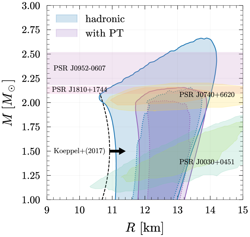
As clear from the M-R curves the two ensemble of EOSs marks two distinctly different contours in the M-R diagram. At low densities the EOSs with first-order PT are stiff compared to the hadronic EOSs (otherwise they cannot satisfy the maximum mass constraint of ). Thus, at lower masses, they have comparatively higher radii [56]. If the PT EOSs are to have softer EOSs at lower densities than after the PT, to satisfy the bound, they need to be uncharacteristically stiffer, thus violating the causality limit. However, for the hadronic EOSs this is not the case as it can initially be softer and later on can be stiff (as they are always continuous) thereby having smaller radius at low mass values. Also, as there is no density discontinuity they can be relatively stiffer (their stiffness can vary greatly) at high densities and thus generate much higher masses.
The characteristic differences in the EOS revealed in the M-R curve are not limited to it. The quasi-normal modes (QNM) (-modes, -modes) also reveal the characteristic feature of the M-R curve of the EOSs. The -mode frequencies for NSs lie at around kHz whereas the -modes frequencies are relatively higher at around kHz. Along with the -mode and -mode frequency, the damping time of the frequencies is also dependent on the EOS. As already seen the M-R contours for the two distinctively different EOS are quite different, it is expected that they would also show up in the QNMs and their damping time.
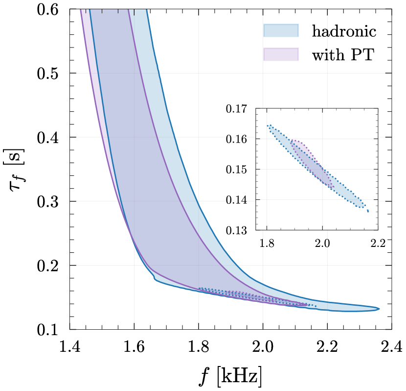
In fig. 2 the plot of damping time against frequency for -mode oscillation is shown. At low frequencies and high damping times there is a difference in the two distinctively different EOS contours; however, this reduces with an increase in the frequency. There is a difference in both the contours and contours. At very high frequencies the contour for both EOS ensembles narrow down. This is due to the fact that we have set a lower mass cut off range for the stars (from observational bounds). For higher masses (beyond ) the number of EOSs reduce proportionally, narrowing down the contours. The incapability of EOSs with first-order PT to produce massive stars (as compared to the hadronic EOSs) ends the contour for the former earlier.
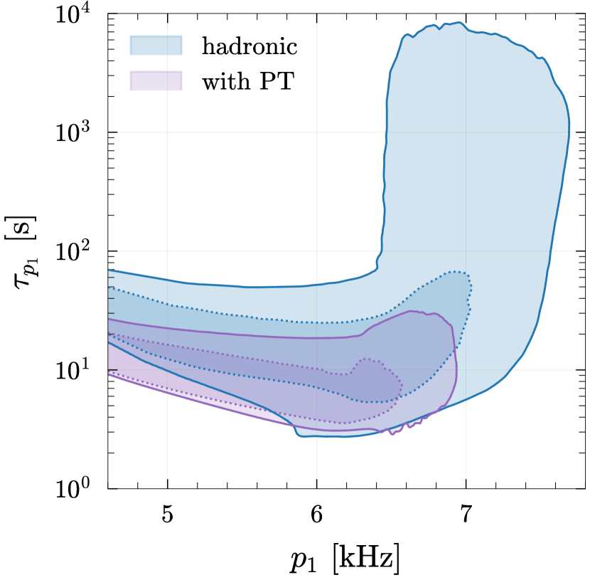
The exclusion regions are more pronounced for the damping time against the frequency plot for -modes fig. 3. At low frequencies, the overlap of both contours and contours is much less pronounced as compared to the -modes. Further, the contours differ extensively at higher frequencies and higher damping times. At higher damping times only the hadronic EOS contour exists. This is as due to the presence of a radial node; p-modes are more sensitive to the distribution of matter inside the star, which is in turn governed by the EOS [7]. Since the hadronic EOSs are much less constrained by the stiffness of the EOS (the variation of stiffness at comparatively higher densities is larger compared to EOS with PT), they can produce more massive stars, and several EOS reach these large values of damping times. While, due to the constraints on the construction of EOSs with PT, very few reach such large values and these don’t show up in the 95% confidence interval.
Universal relations
Recently, there has been extensive use of URs to study matter properties in NSs. It has led to a plethora of URs like I-love-Q, f-love, f-compactness. Usually, these are relations between dimensionless quantities from NS observables like mass, radius, love number, and compactness and are, therefore, insensitive to the details of the EOS. Because of this insensitivity, knowing one parameter is good enough to predict an unknown parameter with which it shares an UR, independent of the microphysics. However, they are quite ineffective in understanding the details of the EOS.
To study quasi-URs of the mode frequency and its damping time one scales these quantities appropriately. The scaling relations are:
| (4) | ||||
| (5) |
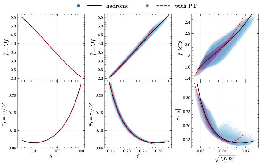
Universality of dimensionless f-mode frequency () and damping time ()is studied with the dimensionless tidal deformability (), compactness () and the average density of the star () in fig. 4. We also study the universality between and in fig. 5.
The log scaled polynomial fitting function used is given by:
| (6) |
where the coefficients are summarized in table 1.
The presence of quasi-universal relations is a purely numerical phenomenon. It’s seen that making specific quantities dimensionless in geometrised units removes the dependence on the EOS, and reduces the spread of the variables. Consequently, using the fitting functions, one can find the value of an unknown quantity (QNM frequency and damping time) if another quantity is known ( or compactness). In the left panel, both the () and axis ( and ) quantities are dimensionless and therefore give a very robust UR without any spread. There is no way to differentiate the two sets of EOS from this UR, as both follow the same relation.
In the middle panel, again, the () and -axis are dimensionless; however, in this case, there is a small spread in both the hadronic and PT EOS sets. At low frequency (and high damping time), the best fit for the UR relation for the two different ensembles of EOS overlaps; however, they deviate slightly at higher frequency (low damping time).
For quantities that are not dimensionless (, and , like the rightmost panel of fig. 4, considerable deviations from the best-fit line exist. Also, the best fit for two different sets of EOS does not always overlap. Interestingly, universality is only prominent in the -modes. -modes do not show universal relations. This violation of universality can be attributed to the fact that they are more sensitive to the matter distribution inside the star, making them more dependent on the EOS.
On the other hand the -modes are manifestations of the average density in the star, which makes them less sensitive to the details of the EOS, and allowing their mass-scaled quantities to show minimum deviations from universality.
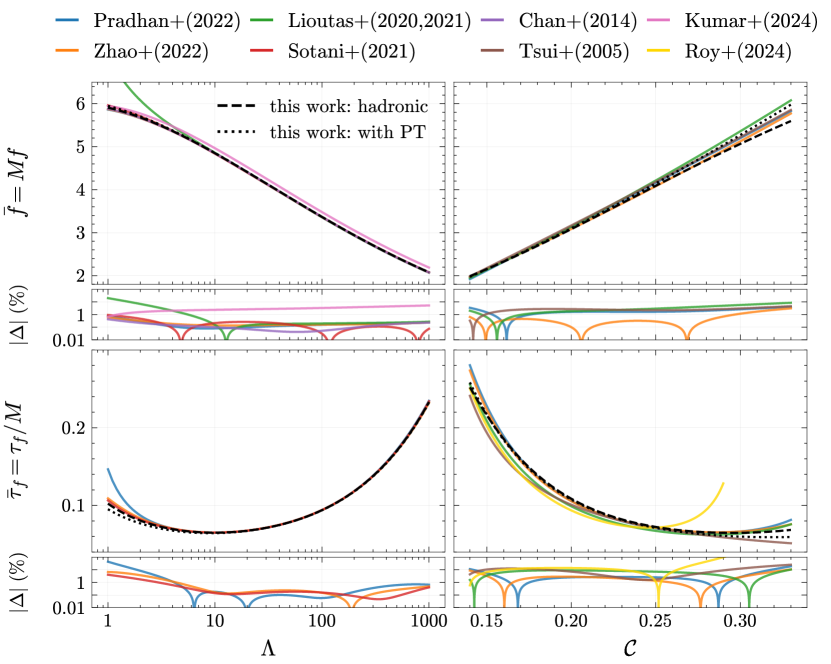
Since the mass scaled -mode frequency () and damping time () individually show universality with and , it is imperative that they also show a universality with each other. This is shown in fig. 5. The mass scaled universal relations have been explored in several previous works which used nuclear EOSs. Our agnostically generated hadronic EOSs are supposed to be a superset of these EOSs, and fig. 6 we show the comparison between our fits and that of other previously reported UR. The amount of deviation of our best-fit from other works are shown below each plot. The EOSs generated by us are generic and are independent of any particular nuclear model, as a result they deviate from others. The coefficients used for fitting our EOSs (both hadronic and PT) are shown in table 1. As the fits from the PT EOSs are similar to those of hadronic EOSs, hence their percentage error for them are also comparable.
| Type | Error% | ||||||
|---|---|---|---|---|---|---|---|
| Max (90%) | |||||||
| Hadronic | 0.7714 | -0.04235 | -0.04707 | 0.003596 | 0.23 (0.10) | ||
| with PT | 0.7744 | -0.04671 | -0.04495 | 0.00326 | 0.55 (0.30) | ||
| Hadronic | -0.9902 | -0.416 | 0.2394 | -0.02033 | 2.21 (0.30) | ||
| with PT | -1.022 | -0.3705 | 0.2181 | -0.01715 | 1.24 (0.60) | ||
| Hadronic | 0.6769 | -1.783 | -4.418 | -2.121 | 6.63 (2.80) | ||
| with PT | 1.412 | 1.289 | -0.1179 | -0.1122 | 5.46 (1.80) | ||
| Hadronic | 3.832 | 23.007 | 33.169 | 14.407 | 11.41 (4.60) | ||
| with PT | 1.775 | 14.187 | 20.584 | 8.444 | 9.95 (3.30) | ||
| Hadronic | 20.827 | 41.24 | 27.989 | 6.435 | 12.92 (6.00) | ||
| with PT | 51.789 | 105.394 | 72.299 | 16.636 | 8.27 (3.80) | ||
| Hadronic | 14.272 | 23.477 | 9.546 | 0.3369 | 54.42 (7.80) | ||
| with PT | 150.459 | 306.473 | 205.458 | 45.524 | 21.86 (7.30) | ||
| Hadronic | -0.3968 | 0.9765 | -7.507 | 6.414 | 14.45 (0.60) | ||
| with PT | -0.1201 | -0.8404 | -3.628 | 3.712 | 5.57 (0.20) |
V Summary and Discussion
Oscillation modes of NS has proven to be a tool of paramount importance in recent years. QNMs in NSs are excited by various mechanisms like accretion, core collapse, and tidal forces due to a close encounter; and can be probed using GWs. The , and - modes having frequencies in the range of a few kHz are of utmost importance due to their possibility of detection in the present and the future detectors.
This work analyses the possibility of probing the internal composition of NSs using and modes. The dependence of the presence or absence of a first-order PT on the and modes are studied. To have an unbiased check of this difference it is necessary to have an exhaustive ensemble of EOS both with and without PT. Two separate ensembles of EOSs are created in an agnostic way that satisfies the astrophysical bounds and is thermodynamically consistent.
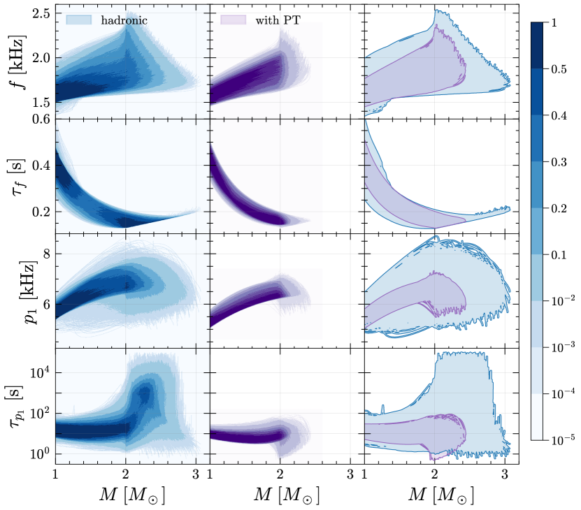
Solving the TOV equations for the ensemble of EOS, one gets a broad contour in the mass-radius curve (plotting and confidence contours). The contours for hadronic EOSs and for PT EOSs differ considerably. The hadronic contour spreads to much larger masses and lower radii than PT contours. This indicates that the PT EOSs are stiffer than hadronic EOS at low densities to fulfill the causal criterion at large densities. This feature is also manifested in their damping time and frequency. Exclusive regions exist for the hadronic and with PT EOS contours and are also more prominent for modes. This is because modes are more sensitive to the matter distribution inside the NS due to the presence of a radial node. It is important to note that the difference in these frequency modes is not due to the priors used for their construction. The contours of both and mode frequencies and damping time with mass (fig. 7) shows us that the hadronic EOSs engulf the entire contour of the PT EOSs. The and intervals highlight that there exists an intrinsic difference that is independent of the priors used for the construction of the EOSs. This has been discussed further in appendix B
URs can largely cater to understanding macroscopic variables, but fail to capture the microphysical elements of NSs. The comparison of URs for hadronic and PT EOSs shows that the exclusive region has no implications on the URs. The fitting functions for both hadronic and PT case with and are similar, indicating that URs cannot be used to differentiate the two types of EOSs. It is also to be noted that the nature of universality depends largely on the dimensionless parameters. Before introducing the dimensionless quantities, the quantities were not universal, implying that the dimensionless quantities can veil several interesting properties of EOSs, thus lacking effectiveness in probing the microscopic properties of NSs.
Although the appearance of exclusion regions is an exciting prospect with which the likelihood of an EOS (hadronic or with PT) can be predicted, they lie in the range of a few kHz. Present GW detectors are not very sensitive to such high frequency, and one thus has to wait for future detectors to study the likelihood of hadronic and PT EOS.
Acknowledgments
The authors would like to thank IISER Bhopal for providing the infrastructure to carry out the research. SC wants to acknowledge the Prime Minister’s Research Fellowship (PMRF), Ministry of Education Govt. of India, for a graduate fellowship. RM is grateful to the Science and Engineering Research Board (SERB), Govt. of India for monetary support in the form of Core Research Grant (CRG/2022/000663). K K Nath would like to acknowledge the Department of Atomic Energy (DAE), Govt. of India, for sponsoring the fellowship covered under the sub-project no. RIN4001-SPS (Basic research in Physical Sciences). The authors would like to thank C. Ecker and L. Rezzolla for providing us with the hadronic EOSs and also for their insights and comments which has helped this project.
References
- Kokkotas and Schutz [1992] K. D. Kokkotas and B. F. Schutz, “W-modes: a new family of normal modes of pulsating relativistic stars,” Monthly Notices of the Royal Astronomical Society 255, 119 (1992), https://academic.oup.com/mnras/article-pdf/255/1/119/18523446/mnras255-0119.pdf.
- Kokkotas and Schmidt [1999] K. D. Kokkotas and B. G. Schmidt, “Quasinormal modes of stars and black holes,” Living Rev. Rel. 2, 2 (1999), arXiv:gr-qc/9909058.
- Zhao and Lattimer [2022] T. Zhao and J. M. Lattimer, “Universal relations for neutron star -mode and -mode oscillations,” Phys. Rev. D 106, 123002 (2022).
- Sathyaprakash et al. [2019] B. Sathyaprakash, A. Buonanno, L. Lehner, C. V. D. Broeck, P. Ajith, A. Ghosh, K. Chatziioannou, P. Pani, M. Puerrer, T. Sotiriou, S. Vitale, N. Yunes, K. G. Arun, E. Barausse, M. Baryakhtar, R. Brito, A. Maselli, T. Dietrich, W. East, I. Harry, T. Hinderer, G. Pratten, L. Shao, N. Tamanini, M. van de Meent, V. Varma, J. Vines, H. Yang, and M. Zumalacarregui, “Extreme gravity and fundamental physics,” baas 51, 251 (2019), arXiv:1903.09221 [astro-ph.HE].
- et al. [2010] M. P. et al., “The Einstein Telescope: a third-generation gravitational wave observatory,” Classical and Quantum Gravity 27, 194002 (2010).
- Kalogera [2021] V. e. a. Kalogera, “The Next Generation Global Gravitational Wave Observatory: The Science Book,” arXiv e-prints , arXiv:2111.06990 (2021), arXiv:2111.06990 [gr-qc].
- Andersson and Kokkotas [1998] N. Andersson and K. D. Kokkotas, “Towards gravitational wave asteroseismology,” mnras 299, 1059 (1998), arXiv:gr-qc/9711088 [gr-qc].
- Yagi and Yunes [2013] K. Yagi and N. Yunes, “I-Love-Q Relations in Neutron Stars and their Applications to Astrophysics, Gravitational Waves and Fundamental Physics,” Phys. Rev. D 88, 023009 (2013), arXiv:1303.1528 [gr-qc].
- Nath et al. [2023] K. K. Nath, R. Mallick, and S. Chatterjee, “I-Love-Q relations for a generic family of neutron star equations of state,” Mon. Not. Roy. Astron. Soc. 524, 1438 (2023), arXiv:2302.05088 [gr-qc].
- Chan et al. [2014] T. K. Chan, Y.-H. Sham, P. T. Leung, and L.-M. Lin, “Multipolar universal relations between -mode frequency and tidal deformability of compact stars,” Phys. Rev. D 90, 124023 (2014).
- Chirenti et al. [2015] C. Chirenti, G. H. de Souza, and W. Kastaun, “Fundamental oscillation modes of neutron stars: validity of universal relations,” Phys. Rev. D 91, 044034 (2015), arXiv:1501.02970 [gr-qc].
- Lioutas et al. [2021] G. Lioutas, A. Bauswein, and N. Stergioulas, “Frequency deviations in universal relations of isolated neutron stars and postmerger remnants,” Phys. Rev. D 104, 043011 (2021).
- Tsui and Leung [2005] L. K. Tsui and P. T. Leung, “Universality in quasi-normal modes of neutron stars,” mnras 357, 1029 (2005), arXiv:gr-qc/0412024 [gr-qc].
- Lioutas and Stergioulas [2018] G. Lioutas and N. Stergioulas, “Universal and approximate relations for the gravitational-wave damping timescale of -modes in neutron stars,” Gen. Rel. Grav. 50, 12 (2018), arXiv:1709.10067 [gr-qc].
- Sotani and Kumar [2021] H. Sotani and B. Kumar, “Universal relations between the quasinormal modes of neutron star and tidal deformability,” Phys. Rev. D 104, 123002 (2021).
- Benhar et al. [2004] O. Benhar, V. Ferrari, and L. Gualtieri, “Gravitational wave asteroseismology reexamined,” Phys. Rev. D 70, 124015 (2004).
- Ranea-Sandoval et al. [2018] I. F. Ranea-Sandoval, O. M. Guilera, M. Mariani, and M. G. Orsaria, “Oscillation modes of hybrid stars within the relativistic Cowling approximation,” Journal of Cosmology and Astroparticle Physics 2018, 031 (2018).
- Jaiswal and Chatterjee [2021] S. Jaiswal and D. Chatterjee, “Constraining dense matter physics using f-mode oscillations in neutron stars,” Physics 3, 302 (2021).
- Aguirre [2022] R. M. Aguirre, “Hyperons, deconfinement, and the speed of sound in neutron stars,” Phys. Rev. D 105, 116023 (2022).
- Flores et al. [2019] C. V. Flores, A. Parisi, C.-S. Chen, and G. Lugones, “Fundamental oscillation modes of self-interacting bosonic dark stars,” Journal of Cosmology and Astroparticle Physics 2019, 051 (2019).
- Pradhan and Chatterjee [2021] B. K. Pradhan and D. Chatterjee, “Effect of hyperons on f-mode oscillations in Neutron Stars,” Phys. Rev. C 103, 035810 (2021), arXiv:2011.02204 [astro-ph.HE].
- Das et al. [2021] H. C. Das, A. Kumar, S. K. Biswal, and S. K. Patra, “Impacts of dark matter on the -mode oscillation of hyperon star,” Phys. Rev. D 104, 123006 (2021).
- Kunjipurayil et al. [2022] A. Kunjipurayil, T. Zhao, B. Kumar, B. K. Agrawal, and M. Prakash, “Impact of the equation of state on f- and p- mode oscillations of neutron stars,” Physical Review D 106, 063005 (2022).
- Pradhan et al. [2022] B. K. Pradhan, D. Chatterjee, M. Lanoye, and P. Jaikumar, “General relativistic treatment of f-mode oscillations of hyperonic stars,” Phys. Rev. C 106, 015805 (2022), arXiv:2203.03141 [astro-ph.HE].
- Ranea-Sandoval et al. [2019] I. F. Ranea-Sandoval, M. G. Orsaria, G. Malfatti, D. Curin, M. Mariani, G. A. Contrera, and O. M. Guilera, “Effects of hadron-quark phase transitions in hybrid stars within the njl model,” Symmetry 11 (2019), 10.3390/sym11030425.
- Gaertig et al. [2011] E. Gaertig, K. Glampedakis, K. D. Kokkotas, and B. Zink, “-mode instability in relativistic neutron stars,” Phys. Rev. Lett. 107, 101102 (2011).
- Krüger and Kokkotas [2020a] C. J. Krüger and K. D. Kokkotas, “Fast rotating relativistic stars: Spectra and stability without approximation,” Phys. Rev. Lett. 125, 111106 (2020a).
- Krüger and Kokkotas [2020b] C. J. Krüger and K. D. Kokkotas, “Dynamics of fast rotating neutron stars: An approach in the hilbert gauge,” Phys. Rev. D 102, 064026 (2020b).
- Doneva et al. [2013] D. D. Doneva, E. Gaertig, K. D. Kokkotas, and C. Krüger, “Gravitational wave asteroseismology of fast rotating neutron stars with realistic equations of state,” Phys. Rev. D 88, 044052 (2013).
- Zink et al. [2010] B. Zink, O. Korobkin, E. Schnetter, and N. Stergioulas, “Frequency band of the -mode chandrasekhar-friedman-schutz instability,” Phys. Rev. D 81, 084055 (2010).
- Yoshida [2012] S. Yoshida, “Nonaxisymmetric oscillations of rapidly rotating relativistic stars by conformal flatness approximation,” Phys. Rev. D 86, 104055 (2012).
- Kastaun et al. [2010] W. Kastaun, B. Willburger, and K. D. Kokkotas, “Saturation amplitude of the -mode instability,” Phys. Rev. D 82, 104036 (2010).
- Passamonti et al. [2013] A. Passamonti, E. Gaertig, K. D. Kokkotas, and D. Doneva, “Evolution of the -mode instability in neutron stars and gravitational wave detectability,” Phys. Rev. D 87, 084010 (2013).
- Pnigouras and Kokkotas [2016] P. Pnigouras and K. D. Kokkotas, “Saturation of the -mode instability in neutron stars. ii. applications and results,” Phys. Rev. D 94, 024053 (2016).
- Rosofsky et al. [2019] S. G. Rosofsky, R. Gold, C. Chirenti, E. A. Huerta, and M. C. Miller, “Probing neutron star structure via -mode oscillations and damping in dynamical spacetime models,” Phys. Rev. D 99, 084024 (2019).
- Baym et al. [1971] G. Baym, C. Pethick, and P. Sutherland, “The Ground State of Matter at High Densities: Equation of State and Stellar Models,” apj 170, 299 (1971).
- Altiparmak et al. [2022] S. Altiparmak, C. Ecker, and L. Rezzolla, “On the sound speed in neutron stars,” The Astrophysical Journal Letters 939, L34 (2022).
- Hebeler et al. [2013] K. Hebeler, J. M. Lattimer, C. J. Pethick, and A. Schwenk, “Equation of state and neutron star properties constrained by nuclear physics and observation,” The Astrophysical Journal 773, 11 (2013).
- Annala et al. [2018] E. Annala, T. Gorda, A. Kurkela, and A. Vuorinen, “Gravitational-wave constraints on the neutron-star-matter equation of state,” Phys. Rev. Lett. 120, 172703 (2018).
- Kurkela et al. [2010] A. Kurkela, P. Romatschke, and A. Vuorinen, “Cold quark matter,” Phys. Rev. D 81, 105021 (2010).
- Oppenheimer and Volkoff [1939] J. R. Oppenheimer and G. M. Volkoff, “On massive neutron cores,” Phys. Rev. 55, 374 (1939).
- Cromartie et al. [2020] H. T. Cromartie, E. Fonseca, S. M. Ransom, P. B. Demorest, Z. Arzoumanian, H. Blumer, P. R. Brook, M. E. DeCesar, T. Dolch, J. A. Ellis, R. D. Ferdman, E. C. Ferrara, N. Garver-Daniels, P. A. Gentile, M. L. Jones, M. T. Lam, D. R. Lorimer, R. S. Lynch, M. A. McLaughlin, C. Ng, D. J. Nice, T. T. Pennucci, R. Spiewak, I. H. Stairs, K. Stovall, J. K. Swiggum, and W. W. Zhu, “Relativistic shapiro delay measurements of an extremely massive millisecond pulsar,” Nature Astronomy 4, 72 (2020).
- Antoniadis et al. [2013] J. Antoniadis, P. C. C. Freire, N. Wex, T. M. Tauris, R. S. Lynch, M. H. van Kerkwijk, M. Kramer, C. Bassa, V. S. Dhillon, T. Driebe, J. W. T. Hessels, V. M. Kaspi, V. I. Kondratiev, N. Langer, T. R. Marsh, M. A. McLaughlin, T. T. Pennucci, S. M. Ransom, I. H. Stairs, J. van Leeuwen, J. P. W. Verbiest, and D. G. Whelan, “A massive pulsar in a compact relativistic binary,” Science 340, 1233232 (2013), https://www.science.org/doi/pdf/10.1126/science.1233232.
- Fonseca [2021] E. e. a. Fonseca, “Refined Mass and Geometric Measurements of the High-mass PSR J0740+6620,” apjl 915, L12 (2021), arXiv:2104.00880 [astro-ph.HE].
- Abbott et al. [2018] B. P. Abbott, R. Abbott, et al. (The LIGO Scientific Collaboration and the Virgo Collaboration), “Gw170817: Measurements of neutron star radii and equation of state,” Phys. Rev. Lett. 121, 161101 (2018).
- Abbott [2019] B. P. e. a. Abbott (LIGO Scientific Collaboration and Virgo Collaboration), “Properties of the binary neutron star merger gw170817,” Phys. Rev. X 9, 011001 (2019).
- Thorne and Campolattaro [1967] K. S. Thorne and A. Campolattaro, “Non-Radial Pulsation of General-Relativistic Stellar Models. I. Analytic Analysis for L = 2,” The Astrophysical Journal 149, 591 (1967).
- Thorne [1969] K. S. Thorne, “Nonradial Pulsation of General-Relativistic Stellar Models. III. Analytic and Numerical Results for Neutron Stars,” apj 158, 1 (1969).
- Chandrasekhar and Ferrari [1991] S. Chandrasekhar and V. Ferrari, “On the non-radial oscillations of a star,” Proceedings of the Royal Society of London Series A 432, 247 (1991).
- Sotani et al. [2001] H. Sotani, K. Tominaga, and K.-i. Maeda, “Density discontinuity of a neutron star and gravitational waves,” Physical Review D 65, 024010 (2001).
- Lindblom and Detweiler [1983] L. Lindblom and S. L. Detweiler, “The quadrupole oscillations of neutron stars,” Astrophysical Journal Supplement Series (ISSN 0067-0049), vol. 53, Sept. 1983, p. 73-92. 53, 73 (1983).
- Detweiler and Lindblom [1985] S. Detweiler and L. Lindblom, “On the nonradial pulsations of general relativistic stellar models,” The Astrophysical Journal 292, 12 (1985).
- Lü and Suen [2011] J.-L. Lü and W.-M. Suen, “Determining the long living quasi-normal modes of relativistic stars,” Chinese Physics B 20, 040401 (2011).
- Cox [1976] J. P. Cox, “Nonradial Oscillations of Stars: Theories and Observations,” Annual Review of Astronomy and Astrophysics 14, 247 (1976).
- Rodriguez et al. [2023] M. C. Rodriguez, I. F. Ranea-Sandoval, C. Chirenti, and D. Radice, “Three approaches for the classification of protoneutron star oscillation modes,” Monthly Notices of the Royal Astronomical Society , stad1459 (2023).
- Gorda et al. [2023] T. Gorda, K. Hebeler, A. Kurkela, A. Schwenk, and A. Vuorinen, “Constraints on Strong Phase Transitions in Neutron Stars,” Astrophys. J. 955, 100 (2023), arXiv:2212.10576 [astro-ph.HE].
- Lioutas and Stergioulas [2020] G. Lioutas and N. Stergioulas, “The gravitational wave damping timescales of f-modes in neutron stars,” Journal of Physics: Conference Series 1667, 012026 (2020).
- Kumar et al. [2024] A. Kumar, M. K. Ghosh, P. Thakur, V. B. Thapa, K. K. Nath, and M. Sinha, “Universal relations for compact stars with exotic degrees of freedom,” The European Physical Journal C 84, 692 (2024).
- Roy et al. [2024] D. G. Roy, T. Malik, S. Bhattacharya, and S. Banik, “Analysis of neutron star f-mode oscillations in general relativity with spectral representation of nuclear equations of state,” The Astrophysical Journal 968, 124 (2024).
- [60] N. Wogan, “odepack,” https://github.com/Nicholaswogan/odepack.
Appendix A Equations governing oscillation modes of a static star
A.1 General relativistic formalism
Lindblom and Detweiller [51, 52] introduced a new fluid perturbation variable , to replace in eq. 3. The Lagrangian pressure variations are related to this new variable by
| (A1) |
One can solve the perturbed Einstein equation, , to get all the relations between the perturbation functions inside the star. To avoid potential singularities in the eigenvalue problem, Lindblom and Detweiller pick the four independent variables to be , , and . The differential equations governing these variables, and the algebraic relations of and are given as follows:
| (A2a) | ||||
| (A2b) | ||||
| (A2c) | ||||
| (A2d) | ||||
| (A2e) | ||||
| (A2f) | ||||
where . The system of differential and algebraic equations, eq. A2 completely describes the perturbations inside the star. It’s clear that the system of differential equations is singular at , and the system blows up rapidly close to the stellar centre. To circumvent this problem, if , then near the center, is approximated as . The forms of and are given in eq. (15) of [53]. These form the initial boundary conditions of the problem. The surface boundary condition is simply that at the surface of the star, the pressure perturbations, and thus must be . To solve eq. A2, we follow the method outlined in [51]. We start off with 3 linearly independent solutions at the surface, and 2 linearly independent solutions at the centre and integrate them backwards and forwards to some point inside the star where they are matched. A linear combination of these solutions, with the coefficients obtained after matching, gives the true values of and at the surface of the star. These variables; and are the only variables defined outside the star, where the perturbation equations reduce to the Zerilli equation [53, 3]:
| (A3) |
where is the Zerilli potential,
| (A4) |
is the tortoise coordinate, , and , with being the total mass of the star.
In case of a first-order with PT in the star, we impose additional junction conditions which ensure the continuity of , , and across the point of discontinuity of energy density [50].
The perturbed metric outside the star describes a combination of outgoing and incoming gravitational waves, which is the general solution to the Zerilli equation. We are interested in the case of purely outgoing waves, representing the QNMs of the star. At the surface of the star, where , the fluid variables can be converted to the Zerilli ones using [3]:
| (A5a) | ||||
| (A5b) | ||||
Here
| (A6a) | ||||
| (A6b) | ||||
| (A6c) | ||||
After continuing the integration of the Zerilli equation eq. A3 to sufficiently far away from the star (), the solution can be approximated as a linear combination of incoming and outgoing waves as where represents the outgoing wave, the incoming wave and and their amplitudes. At a large enough radius,
| (A7a) | ||||
| (A7b) | ||||
Here is the complex conjugate of (and hence the complex conjugate of ) and, [3]
| (A8a) | ||||
| (A8b) | ||||
can be any complex number that represents an overall phase. By matching the solution of and obtained from eq. A5 with the above equation, we can find the amplitude with a simple matrix inversion [3]. The frequency of the QNM corresponds to that which minimises .
To find the QNM frequency and its damping time we first find , which in general will be a complex number, for several real values of close to the original guess. We then perform a complex polynomial fitting to approximate a parabola passing through the points corresponding to the values. The root of this parabola which has a positive imaginary part is the required complex of our QNM. We then take the real part of this and repeat the entire procedure several more times till the desired tolerance is reached. The real part of this final is the frequency of the QNM. The inverse of the imaginary part is the corresponding damping time.
For the initial guess, we use Brent’s method to find all minimas of . By checking the number of radial nodes of the fluid variables, as well as by comparing the values of the minimas with each other, it can be found which minima corresponds to which fluid oscillation mode ( or ). These minimas are then taken to be the initial guesses for the corrsponding mode.
A.2 Notes on computation
The numerical integration of all relevant ODEs was performed using an ODE solver, LSODA, which automatically adjusts the step size and switches between non-stiff (Adam’s) and stiff (BDF) methods. We further used a thread-safe version of this algorithm [60] so that we can run our code in parallel on multiple threads, significantly reducing the computation time required for the large number of EOSs in this work. We specified the relative tolerance to be and the absolute tolerance to be throughout the code; and obtained satisfactory results. The validity of our code was checked thoroughly by comparing our results with those in several previous works [23, 50]. Moreover, we also calculated the oscillation modes and damping times using Thorne [48] Ferrari’s [49] Breit-Wigner resonance fitting approach and the frequency values matched those obtained by the Lindblom [51, 52] approach.
Appendix B Sampling technique
The ensemble of EOSs generated in this work uses two different priors. It is essential to understand whether the distinct exclusion region for the and contours is due to our sampling technique. The contours are obtained from the corresponding probability density functions (PDFs). To find these, we divide the plane into a fixed-resolution grid and count the number of curves passing through each grid cell. To smoothen the distribution, we apply a 1 gaussian filter. Finally, we normalize the distribution by dividing all cell counts by the maximum count. The resulting PDFs and the 100% contours for the frequency and damping time with mass are shown in fig. 7. In fig. 7 (right panels) we show the entire contour corresponding to the damping time vs masses for both and modes. The figures show that the PT EOSs all lie within the contour of the hadronic EOSs for both cases. Any existing bias that might arise due to the different sampling techniques of our EOSs would have resulted in two separate contours consisting of an exclusion region even for the 100%