Neutrino beaming in ultraluminous X-ray pulsars as a result of gravitational lensing by neutron stars

Abstract

X-ray pulsars experiencing extreme mass accretion rates can produce neutrino emission in the MeV energy band. Neutrinos in these systems are emitted in close proximity to the stellar surface and subsequently undergo gravitational bending in the space curved by a neutron star. This process results in the formation of a distinct beam pattern of neutrino emission and gives rise to the phenomenon of neutrino pulsars. The energy flux of neutrinos, when averaged over the neutron star’s pulsation period, can differ from the isotropic neutrino energy flux, which impacts the detectability of bright pulsars in neutrinos. We investigate the process of neutrino beam pattern formation, accounting for neutron star transparency to neutrinos and gravitational bending. Based on simulated neutrino beam patterns, we estimate the potential difference between the actual and apparent neutrino luminosity. We show that the apparent luminosity can greatly exceed the actual luminosity, albeit only in a small fraction of cases, depending on the specific equation of state and the mass of the star. For example, the amplification can exceed a factor of ten for $\approx 0.2\%$ of typical neutron stars with mass of $1.4\,M_{\odot}$. Strong amplification is less probable for neutron stars of higher mass. In the case of strange stars, a fraction of high energy neutrinos can be absorbed and the beam pattern, as well as the amplification of apparent neutrino luminosity, depend on neutrino energy.

1 Introduction

X-ray pulsars (XRPs) are accreting neutron stars (NSs) in close binary systems (see Mushtukov & Tsygankov 2022 for review). Typical field strength at the NS surface here is expected to be $\sim 10^{12}\,{\rm G}$ or even stronger. Such a strong magnetic field modifies the geometry of accretion flow directing it towards small regions located close to the poles of a NS and dramatically influences elementary processes of radiation/matter interaction (see Harding & Lai 2006). The luminosity of XRPs is powered by the accretion process, the most efficient mechanism of energy release. The apparent luminosity of XRPs covers about nine orders of magnitude. The lowest detected luminosity is known to be $\sim 10^{32}\,{\rm erg\ \rm s^{-1}}$. The brightest XRPs show luminosity $\gtrsim 10^{40}\,{\rm erg\ \rm s^{-1}}$ and belong to the class of ultra-luminous X-ray sources (see, Bachetti et al. 2014; Israel et al. 2017, and Fabrika et al. 2021 for review). The geometry of the emission regions at the NS surface is expected to be dependent on the mass accretion rate (Basko & Sunyaev, 1975). At a relatively low mass accretion rate ($\lesssim 10^{17}$ g s^-1), the accretion flow reaches the stellar surface and is decelerated in the atmosphere of a NS due to the Coulomb collisions, which leads to the formation of hot spots located close to magnetic poles of a star. At higher mass accretion rates, the luminosity of a NS is sufficiently high ($\gtrsim 10^{37}\,{\rm erg\ \rm s^{-1}}$) to cause radiative force that stops accretion flow above the stellar surface. It leads to the formation of accretion columns – extended structures confined by a strong magnetic field and supported by the radiation pressure gradient (Wang & Frank, 1981; Mushtukov et al., 2015; Zhang et al., 2022). At mass accretion rates exceeding $\sim 10^{19}\,{\rm g\,s^{-1}}$, accretion columns can be advective, i.e. X-ray photons are confined inside a sinking region due to large optical thickness of the flow (Mushtukov et al., 2018b). Under this condition, the temperature of plasma can be as high as a few hundred keV, which is sufficient to cause intense creation of electron-positron pairs (Mushtukov, Ognev & Nagirner, 2019) and further neutrino emission due to their annihilation (Kaminker et al., 1992). Thus, bright XRPs can manifest themselves as sources of intense neutrino emission, where the total energy flux released due to accretion is channelled into luminosity in photons and luminosity in neutrinos. The intrinsic neutrino luminosity of a NS is maximal right after the supernova explosion and then decreases rapidly with time: it is expected to be $<10^{37}\,{\rm erg\ \rm s^{-1}}$ ($<10^{36}\,{\rm erg\ \rm s^{-1}}$) after a ${\rm few}\times 10^{2}$ years ($10^{3}$ years) after the explosion (Yakovlev et al., 2005), which is well below the expected neutrino luminosity in bright ULXs.

The higher the mass accretion rate and the total luminosity, the larger the fraction of energy released in the form of neutrinos (see Fig. 1 in Asthana et al. 2023). The highest neutrino luminosity is expected in ULX pulsars, if their apparent luminosity is close to the actual one (see, e.g., King, Lasota & Kluźniak 2017, where the authors show that it is not necessarily the case, and Mushtukov et al. 2021; Mushtukov & Portegies Zwart 2023, where an opposite point of view is presented). Due to the extra-galactic nature of confirmed ULX pulsars, the expected neutrino flux is very low and even expected to be significantly below the neutrino isotropic background in a MeV energy band (Asthana et al., 2023). However, recent estimations of neutrino flux from ULX pulsars (see Asthana et al. 2023) were performed under the assumption of isotropic neutrino emission, which can be violated by initial non-isotropic emission as well as by gravitational bending of particle trajectories.

In this paper, we investigate neutrino beam pattern formation accounting for neutrino propagation in a space curved by the gravity of a star and transparency of a star for neutrino emission. The gravitational bending results in a difference between actual (initially generated) $L_{\nu}$ and apparent $L_{\nu,\rm app}$ neutrino luminosities. The latter can be different for different distant observers. On the base of calculated beam patterns we obtain expected distributions of neutrino pulsars over the amplification factor

$$a_{\nu}\equiv\frac{L_{\nu,\rm app}}{L_{\nu}}.$$ (1)

2 Model set up

2.1 Equation of state and structure of a neutron star

We assume the NS structure to be spherical. Appreciable deviations from the spherical symmetry can be caused by ultra-strong magnetic fields ($B\gtrsim 10^{17}$ G) or by rotation with ultra-short periods (less than a few milliseconds; see, e.g., Haensel, Potekhin & Yakovlev 2007 and references therein), but we will not consider such cases. For a spherically symmetric and quasi-static mass distribution, metric can be written in the form (e.g., Misner, Thorne & Wheeler, 1973; Thorne, 1977)

$$\mathrm{d}s^{2} = -e^{2\Phi/c^{2}}\mathrm{d}t^{2}+\big{[}1-R_{\mathrm{Sch}}(M_{r})/r\big{]}^{-1}\mathrm{d}r^{2}$$ (2)

$$+r^{2}(\mathrm{d}\theta^{2}+\sin^{2}\theta\,\mathrm{d}\phi^{2}),$$

where $t$ is the time coordinate, $r$, $\theta$ and $\phi$ are the spherical polar coordinates, $M_{r}$ is the gravitational mass inside a sphere of radius $r$,

$$R_{\mathrm{Sch}}(M_{r})\equiv 2GM_{r}/c^{2}$$ (3)

represents the Schwarzschild radius corresponding to the mass $M_{r}$, $G$ is the Newtonian constant of gravitation, $\Phi$ is the gravitational potential and $c$ is the speed of light in a vacuum. Then the mechanical structure of a NS is governed by four first-order differential equations for $r$, $M_{r}$, $\Phi$ and the local pressure $P$ as functions of baryon number $\beta$ inside a given spherical shell (e.g., Richardson, van Horn & Savedoff, 1979):

$$\frac{\mathrm{d}r}{\mathrm{d}\beta} = \frac{1}{4\pi r^{2}\bar{n}}\,\left(1-\frac{R_{\mathrm{Sch}}(M_{r})}{r}\right)^{1/2},$$ (4)

$$\frac{\mathrm{d}M_{r}}{\mathrm{d}\beta} = \frac{\rho}{\bar{n}}\,\left(1-\frac{R_{\mathrm{Sch}}(M_{r})}{r}\right)^{1/2},$$ (5)

$$\frac{\mathrm{d}\Phi}{\mathrm{d}\beta} = G\,\frac{M_{r}+4\pi r^{3}P/c^{2}}{4\pi r^{4}\bar{n}}\,\left(1-\frac{R_{\mathrm{Sch}}(M_{r})}{r}\right)^{-1/2},$$ (6)

$$\frac{\mathrm{d}P}{\mathrm{d}\beta} = -\left(\rho+\frac{P}{c^{2}}\right)\,\frac{\mathrm{d}\Phi}{\mathrm{d}\beta},$$ (7)

where $\bar{n}$ is the mean number density of baryons. We integrate these equations from $r=0$ and $M_{r}=0$ at the center of the star outwards, starting from a predefined baryon density $\bar{n}$ at the center, until a predefined mass density at the outer boundary $\rho_{\mathrm{b}}$ is reached. Since the outermost non-degenerate layers are unimportant for the problem of neutrino propagation to be studied, we restrict ourselves by the strongly degenerate matter. This allows us to use a barotropic equation of state (EoS), which provides mass density $\rho$ and pressure $P$ as functions of $\bar{n}$, regardless of temperature.

The boundary condition for $\Phi$ is provided by the Schwarzschild metric outside the star,

$$\mathrm{e}^{2{\Phi_{\mathrm{b}}/c^{2}}}=1-\frac{2GM}{Rc^{2}},$$ (8)

where $R$ and $M=M_{R}$ are the stellar radius and mass, and $\Phi_{\mathrm{b}}$ is the value of $\Phi(\beta)$ at the stellar surface. Since the value of $\Phi$ at the center of the NS is not known in advance, we integrate Eq. (6) for a shifted potential $\tilde{\Phi}(\beta)=\Phi(\beta)-\Phi(0)$, with the initial value $\tilde{\Phi}(0)=0$ at the center of the star, and the value of the shift $\Phi(0)$ is found from Eq. (8) after the integration has been completed.

We solve the set of equations (4) – (7) numerically by the Runge-Kutta method on a non-uniform grid in $\beta$, with variable steps adapted to provide a sufficient accuracy at each grid node for each of the computed functions. We decrease each step until a desired accuracy is reached. In order to prevent accuracy loss in the outer layers of the star, where $\beta$ is nearly constant as a function of $\rho$ or $r$, we use the difference $(\beta_{\mathrm{b}}-\beta)$ as an independent variable, $\beta_{\mathrm{b}}$ being the boundary value of $\beta$, equal to the total number of baryons in the NS.

We limit ourselves to three EoSs: APR (Akmal, Pandharipande & Ravenhall, 1998), SLy4 (Douchin & Haensel, 2001) and BSk24 (Pearson et al., 2018). These EoSs describe the ground state for the nucleon-lepton ($npe\mu$) composition of matter, which is the most conservative assumption, without any “exotic” constituents. The APR EoS for the NS core is based on realistic effective two- and three-nucleon interactions, which allow one to reproduce various nucleon scattering data and the properties of light nuclei. We adopt the version of the APR EoS named A18+$\delta{v}$+UIX^∗ in Akmal et al. (1998), which includes a relativistic boost correction, in the parametrized form of Potekhin & Chabrier (2018). This parametrization includes the NS crust described by the BSk24 EoS on top of the core described by the APR EoS. The SLy and BSk models are based on effective nucleon-nucleon interactions of the Skyrme type, adjusted to reproduce the EoS of pure neutron matter and the experimental properties of heavy atomic nuclei. These EoS models are unified: they are based on the same microscopic models for the core and the crust. For the first (SLy) EoS family, we use the SLy4 EoS in the parametrized form of Haensel & Potekhin (2004). The more recent BSk interaction model is more complicated; it is better tuned to the recent collection of experimental nuclear data. The BSk24 and BSk25 versions of this model, which are very similar, appear to be preferred, as discussed by Pearson et al. (2018). The BSk24 EoS is substantially stiffer than the SLy4 EoS, and we choose them as representative examples of relatively stiff and soft EoS models.

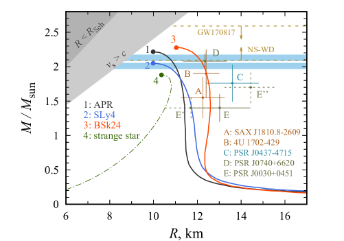
Figure 1: NS mass $M$ versus radius $R$ for four EoS models compared with theoretical and observational constraints and estimates. The solid curves labelled with numbers 1–3 show mass-radius relation for APR (1), SLy4 (2) and BSk24 (3) EoS models, respectively. The dark-green dashed-dotted line shows an example of mass-radius relation for a strange star. The curves are truncated at the hydrostatic stability limits, marked by the heavy dots. The dark and light grey shaded triangles are prohibited by General Relativity and causality. The horizontal light-blue regions correspond to the mass estimates (with $1\sigma$ uncertainties) for PSR J0348+0432 (the lower one) and PSR J1810+1744 (the upper one). The horizontal dashed lines with arrows mark the upper and lower 3$\sigma$ limits to the maximum NS mass, derived from observations. The error bars show the 1$\sigma$ confidence intervals in $M$ and $R$, inferred from observations of five NSs in binary systems, marked by the letters from A through E, according to the legend (see text for details).

We also consider a possibility of the EoS of strange matter built of the $u,\,d$ and $s$ quarks (Witten, 1984; Haensel, Zdunik & Schaefer, 1986; Alcock, Farhi & Olinto, 1986). For the strange matter EoS, we use the approximation proposed by Zdunik (2000) and adopt the fiducial parameters in his paper: the bag constant $B=60$ MeV fm^-3, the QCD coupling constant $\alpha_{c}=0$ and the rest energy of the strange quark $m_{s}c^{2}=100$ MeV.

The solid curves in Fig. 1 show gravitational mass $M$ versus circumferential radius $R$ of a NS for the three selected EoSs. The dot-dashed curve displays $M(R)$ for a strange star model. The dark grey shaded area ($R<R_{\mathrm{Sch}}(M)$) is prohibited by General Relativity. The entire grey shaded triangle is prohibited by General Relativity combined with the condition that the speed of sound must be subluminal (e.g., section 6.5.7 of Haensel et al. 2007).

The light-blue horizontal bands correspond to the two most accurate estimates of NS masses exceeding 2 M_⊙: PSR J0348+0432 ($M=2.01\pm 0.04$ M_⊙; Antoniadis et al. 2013) and PSR J1810+1744 ($M=2.13\pm 0.04$ M_⊙; Romani et al. 2021). The lower horizontal dashed line with the upward arrow marks the lower 3$\sigma$ limit to the maximum NS mass, $M_{\mathrm{max}}>2.09$, obtained by Romani et al. (2022) jointly for seven heaviest known NSs in binaries with white dwarfs (WDs), including the above-mentioned ones. We note that the mass estimate for PSR J0348+0432 (the lower light-blue band), which was obtained using a combination of the binary mass function and a measurement of the Shapiro delay of the pulsar signal, appears to be less model-dependent than the other mentioned estimates, which were obtained by an analysis of orbital light curves using a WD heating model.

Rezzolla, Most & Weih (2018) used quasi-universal relations exhibited by equilibrium solutions of rotating relativistic stars to infer constraints on the maximum NS mass from an analysis of the electromagnetic and gravitational wave signals from the double NS merger GW170817. Their most conservative upper limit $M_{\mathrm{max}}<2.59$ M_⊙ is shown in Fig. 1 by the upper horizontal dashed line with the downward arrow. It relies on the assumption that the merger product in GW170817 has collapsed into a black hole. However, the kilonova produced in this event could also be explained in an alternative scenario of NS stripping without black hole formation (Blinnikov et al., 2022). Thus the indicated limit is model-dependent.

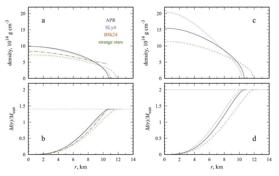
Figure 2: Mass density (a,c) and mass (b,d) distributions inside a NS/strange star of a given total mass and EoS. Different curves are calculated for different EoS: APR (black solid), SLy4 (blue dotted), BSk24 (red dashed), and EoS for a strange star according to Zdunik (2000). Mass of a NS is fixed at $M=1.4M_{\odot}$ at panels “a” and “b”, and at $M=2M_{\odot}$ at panels “c” and “d”. Mass of a strange star was taken to be $M=1.4M_{\odot}$ at panel “a”.

The vertical and horizontal error bars in Fig. 1 show the available 1$\sigma$ confidence intervals in $M$ and $R$, respectively, for the cases where these uncertainties are not large ($\la 15$%). The labels A and B mark such intervals for the bursters SAX J1810.8–2609 and 4U 1702-429, according to the analysis by Nättilä et al. (2017). The label C corresponds to the nearest and brightest millisecond pulsar PSR J0437–4715 in an NS-WD binary system. Its mass $M=1.76\pm 0.20$ M_⊙ was constrained using a combination of the mass function and the Shapiro delay by Verbiest et al. (2008), and its radius $R=13.6^{+0.9}_{-0.8}$ km was derived from a spectral analysis by González-Caniulef, Guillot & Reisenegger (2019). Labels D and E mark the results obtained for PSR J0740+6620 (Miller et al., 2021) and PSR J0030+0451 (Miller et al., 2019), respectively, using an analysis of the energy-dependent thermal X-ray waveform observed by NICER. Despite the belief that this approach was “less subject to systematic errors than other approaches for estimating neutron star radii” (Miller et al., 2019), a subsequent reanalysis, performed for PSR J0030+0451 by Vinciguerra et al. (2024) with alternative hot spot models and using jointly the data of NICER and XMM-Newton, resulted in substantially different estimates, shown in Fig. 1 by the dashed error bars and marked as E^′ and E^′′, which demonstrate the strong model dependence. Other joint mass and radius estimates obtained from spectral analyses of X-ray radiation of neutron stars exhibit similar model dependence and are not plotted here (e.g., Tanashkin et al. 2022; see also discussion and references in Potekhin et al. 2020).

Fig. 1 demonstrates that the selected EoS models are reasonably compatible with the available observational NS mass and radius estimates, although the softest SLy4 EoS is only marginally compatible with the lower limits to $M_{\mathrm{max}}$.

Solutions of the stellar structure equations for the three selected NS EoSs are illustrated in Fig. 2. The upper and lower panels show respectively mass density $\rho$ and gravitational mass distributions $M_{r}$ as functions of $r$ for the total mass of a NS equal to $1.4\,M_{\odot}$ (left panels) or $2\,M_{\odot}$ (right panels). The dot-dashed line in the left panels show analogous distributions for the model of a strange star with $M=1.4\,M_{\odot}$.

2.2 Neutrino emission and propagation

The distinct feature of neutrino propagation near a NS stems from the fact that NSs are typically transparent to neutrino emissions of relatively low energy (Sawyer & Soni, 1979; Haensel & Jerzak, 1987), unless their internal temperature exceeds $\sim 1\,{\rm MeV}$, which occurs only immediately following a supernova explosion (see Fig. 2 in Yakovlev et al. 2005). In bright XRPs, it is expected that neutrinos are emitted near the base of the accretion column. We assume that the NS’s magnetic field is predominantly characterized by the dipole component, leading to neutrinos being initially emitted near the magnetic poles of the NS located diametrically opposite on the stellar surface. The primary process of neutrino production involves the annihilation of electron-positron pairs, although a fraction of neutrinos can also be generated via the synchrotron process (see, e.g., Kaminker et al. 1992 and Mushtukov et al., in prep.). Emitted neutrinos propagate both outside and inside the NS, which is cold enough to be transparent or nearly transparent to them. All emitted neutrinos undergo gravitational bending in curved space-time. Neutrino emission and their subsequent propagation along curved trajectories form a distinct beam pattern. While the vast majority of neutrinos initially emitted at the NS surface are of electron flavor, the composition of the neutrino flux varies as it propagates, because of neutrino oscillations. Neutrinos of high energy may experience scatterings in the core of the NS, which influence the trajectories of particles and, consequently, their final angular distribution.

The primary processes governing neutrino opacity in dense matter are neutrino-neutron scattering (see, e.g., Shapiro & Teukolsky 1983 and Fig. 3 in Vantournhout, Jachovicz & Ryckebusch 2006)

$$n+\nu_{e,\mu}\,\longrightarrow\,n+\nu_{e,\mu}.$$ (9)

and neutrino absorption

$$n+\nu_{e}\,\longrightarrow p+e^{-},\qquad n+\nu_{\mu}\,\longrightarrow p+\mu^{-}.$$ (10)

These processes are strongly suppressed in the case of relatively low temperatures because of the degeneracy of the nucleons (see, e.g., Sawyer & Soni 1979; Haensel & Jerzak 1987). The neutrino mean free path in the elastic limit of neutrino-neutron scattering (9) for non-degenerate nucleons can be estimated as (e.g., equation (11.7.8) in Shapiro & Teukolsky, 1983)

$$\overline{\lambda}_{\rm sc,0}\sim 3\,\frac{\rho_{\rm nuc}}{\rho}\left(\frac{\mbox{1~{}MeV}}{E_{\nu}}\right)^{2}\mbox{~{}km},$$ (11)

where $\rho_{\rm nuc}\approx 2.5\times 10^{14}\,{\rm g\,cm^{-3}}$ denotes the mass density at the saturation number density $n_{\mathrm{nuc}}\approx 0.15$ fm^-3 (Horowitz, Piekarewicz & Reed, 2020), $\rho$ is the local mass density, and $E_{\nu}$ stands for the energy of neutrinos. Since the mass density in the NS core substantially exceeds $\rho_{\rm nuc}$, the mean free path of high-energy neutrinos may be smaller than the radius of a NS. Consequently, a portion of neutrinos undergoes scatterings before escaping from a hot NS. However, at temperatures $\lesssim 10\,{\rm keV}$ and densities $\rho\gtrsim\rho_{\rm nuc}$, typical for mature NSs, the neutrino energies most relevant for the ULXs ($E_{\nu}\sim 0.1-1$ MeV) are large compared with temperature but small compared with neutron Fermi energy. Under these conditions, the mean free path can be estimated from equation (26) in Sawyer & Soni (1979),

$$\overline{\lambda}_{\rm sc}\approx 800\left(\frac{\mbox{1~{}MeV}}{E_{\nu}}\right)^{3}\mbox{~{}km},$$ (12)

so that $\overline{\lambda}_{\rm sc}\gg R$.

The neutrino absorption process (10) is forbidden in the degenerate NS matter at $p_{\mathrm{Fn}}\gg p_{\mathrm{Fp}}+p_{\mathrm{Fe}}$ (for the same reason as the direct Urca process; cf., e.g., section 11.2 in Shapiro & Teukolsky 1983), where $p_{\mathrm{F(n,p,e)}}$ are the Fermi momenta of neutrons, protons and electrons, respectively. Thus in the bulk of a typical NS absorption of neutrinos proceeds (in analogy with the modified Urca processes) via the modified reactions $n+n+\nu_{e}\,\longrightarrow p+n+e^{-}$ and $n+p+\nu_{e}\,\longrightarrow p+p+e^{-}$, with the mean free paths still longer than $\overline{\lambda}_{\rm sc}$ at the low temperatures (cf. Haensel & Jerzak, 1987). In this case we can estimate the neutrino mean free path before absorption, $\overline{\lambda}_{\mathrm{abs}}$, using equations (23) and (25) in Haensel & Jerzak (1987). For example, at $E_{\nu}\sim 100$ keV, $\rho\sim 10^{15}$ g cm^-3 and temperature $\sim 10^{8}$ K we obtain $\overline{\lambda}_{\mathrm{abs}}\sim 10^{5}$ km. Equation (16) in Sawyer & Soni (1979) gives a similar result.

If the NS core contains quark matter, neutrino scattering is less efficient than absorption by quarks (see, e.g., Pal & Dutt-Mazumder 2011)

$$d+\nu_{e}\to u+e^{-},$$ (13)

i.e. $\overline{\lambda}_{\rm qabs}/\overline{\lambda}_{\rm qsc}\ll 1$, where $\overline{\lambda}_{\rm qabs}$ and $\overline{\lambda}_{\rm qsc}$ are electron neutrino mean free path due to absorption and scattering in quark matter respectively. The electron neutrino mean free path due to the absorption for $E_{\nu}\sim 500\,{\rm keV}$ can be estimated as

$$\overline{\lambda}_{\rm qabs}\approx\frac{\pi^{4}}{4\,\alpha_{s}\cos^{2}\theta_{c}}\frac{1}{G_{\rm F}^{2}\mu_{d}\mu_{u}\mu_{e}E_{\nu}^{2}}\approx{\color[rgb]{0,0,0}56\,{\rm km},}$$ (14)

where $G_{\rm F}$ is the Fermi weak-coupling constant, $\theta_{c}$ is the Cabibbo angle, and the numerical estimation is based on the typical parameters for quarks in the core of a compact star $\mu_{d}\approx\mu_{u}\approx 500$ MeV, $\mu_{e}\approx 11$ MeV and $\alpha_{s}\approx 1$ (see, e.g., Schäfer & Schwenzer 2004). Based on equation (14), we use the estimate

$$\overline{\lambda}_{\rm qabs}\sim 14\,\left(\frac{\mbox{1~{}MeV}}{E_{\nu}}\right)^{2}\mbox{~{}km}.$$ (15)

To characterize the geometry of spacetime around a NS, we employ the Schwarzschild metric, which serves as a suitable approximation for NSs in XRPs with typical spin periods $P_{\rm spin}\ga 0.1\,{\rm s}$. For a spherically symmetric NS in a hydrostatic equilibrium, metric (2) is locally similar to the Schwarzschild metric produced by mass $M_{r}$. In this metric, trajectories of photons and neutrinos between potential scattering events lie in the same plane. Within the particle trajectory plane, we parameterize the trajectory using polar coordinates, with $r\geq 0$ and $\varphi\in[0,2\pi]$. The trajectory is determined by the differential equation (Misner et al., 1973):

$$\frac{{\rm d}^{2}u}{{\rm d}\varphi^{2}}=3u^{2}-u,$$ (16)

where $u=0.5R_{\rm Sch}(M_{r})/r$. Consequently, trajectories of neutrinos propagating through a NS are contingent upon the mass distribution within the star and are thus anticipated to vary for different EoSs.

2.3 Neutron star rotation and luminosity distribution

The apparent luminosity of a NS can be determined as

$$L_{\rm\nu,app}=\frac{4\pi D^{2}}{T}\int\limits_{0}^{T}F_{\nu}(t){\rm d}t,$$ (17)

where $F_{\nu}(t)$ is variable neutrino energy flux density (as registered by a distant observer), which varies with time $t$, $D$ is a distance to the compact object and $T$ is a time interval. In practice, the integration in (17) is performed over a long time interval ($T\gg P_{\rm spin}$) because the mass accretion rate in X-ray binaries is known to be fluctuating over a wide range of time scales, which should result in fluctuating pulse profiles in X-rays and neutrinos. The ratio of the apparent and actual neutrino luminosity determines the neutrino amplification factor $a_{\nu}$, Eq. (1).

Apparent neutrino luminosity depends on actual neutrino luminosity, neutrino beam pattern and geometry of NS rotation in the observer’s reference frame. Rotation of a NS in the observer’s reference frame is described by two angles: inclination $i$ (i.e., the angle between the rotation axis and observer’s line of sight) and the magnetic obliquity $\theta_{B}$ (i.e., the angle between the rotational and magnetic axis of a NS). The flux is related to the neutrino flux distribution in the reference frame of a NS, which depends on the angle $\psi$ between the observer’s line of sight and NS magnetic axis at a given phase $\varphi_{\rm p}\in[0;2\pi]$ of NS rotation:

$$\cos\psi=\cos i\cos\theta_{B}+\sin i\sin\theta_{B}\cos\varphi_{\rm p}.$$ (18)

The angles $i$ and $\theta_{B}$ are typically unknown for the XRPs. Recent observation of X-ray polarization variable over NS spin period, however, shed light on rotation geometry in some particular accreting strongly magnetized NSs (Doroshenko et al., 2022; Tsygankov et al., 2022, 2023; Doroshenko et al., 2023; Mushtukov et al., 2023; Malacaria et al., 2023; Heyl et al., 2023), but features of NS distribution over rotation parameters are still uncertain. To estimate possible deviations of apparent neutrino luminosity from the actual one, we assume a random distribution of NSs over the parameters of their rotation, simulate neutrino pulse profiles for various rotation parameters and calculate theoretical distributions $f(a_{\nu})$ of NSs over the apparent neutrino luminosity amplification factors $a_{\nu}$. The technique used here is similar to the one applied to investigate distributions of XRPs over the apparent luminosity in X-rays (see, e.g. Mushtukov et al. 2021; Markozov & Mushtukov 2024).

3 Numerical model

Our numerical model consists of two parts. First, we compute the angular distribution of neutrino flux in the reference frame of a NS accounting for neutrino propagation along curved trajectories and scattering/absorption inside a star. Then, using the computed angular distribution, we simulate neutrino flux variability in the observer’s reference frame due to the rotation of a NS and calculate the theoretical distribution of neutrino pulsars over the neutrino amplification factor.

3.1 Neutrino angular distribution

To obtain the angular distribution of neutrinos, we specify neutrino energy $E_{\nu}$, NS EoS and mass, which gives us NS radius and internal mass distribution. Then we perform Monte Carlo simulations and calculate trajectories of $4\times 10^{7}$ particles in each run. There are a few steps in our Monte Carlo simulation:

1. We start with neutrino of energy $E_{\nu}$ emitted from the surface of a NS near one of its magnetic poles. The initial direction of particle motion is taken to be random and calculated under the assumption that the initial angular distribution of neutrinos is isotropic.

2. We choose a random realization of the optical depth traveled by the particle before scattering or absorption event (the dimensionless free path) according to the formula $\tau_{X}=-\ln X,$ where $X\in(0;1)$ is a random number having the uniform distribution.

3. We simulate a particle trajectory by solving numerically differential equation (16) for a set of initial parameters (see Appendix A). If the trajectory crosses the star, we calculate an optical depth traveled by the particle, $\tau_{\nu}$, by integration along the simulated trajectory,

   $$\tau_{\nu}(s)=\int\limits_{0}^{s}\frac{{\rm d}s^{\prime}}{{\color[rgb]{0,0,0}\overline{\lambda}}(s^{\prime})},$$ (19)

   where $s$ is the length along the particle trajectory and

   $$\overline{\lambda}=\frac{1}{\overline{\lambda}_{\mathrm{sc}}^{-1}+\overline{\lambda}_{\mathrm{abs}}^{-1}}$$ (20)

   is the mean free path accounting for scattering ($\overline{\lambda}_{\mathrm{sc}}$) and absorption ($\overline{\lambda}_{\mathrm{abs}}$), which depend on neutrino energy $E_{\nu}$ and mass density $\rho$ at each given point along the path inside the star according to the estimates in Section 2.2. The optical depth (19) is a non-decreasing function, bounded from above by some maximum value for every simulated trajectory. If $\tau_{X}$ exceeds this maximum, the particle goes to infinity without scattering/absorption and we account for its final momentum direction in the simulated angular distribution function. Then we return to step 1 and start the simulation for the next particle. Otherwise, $\tau_{\nu}(s)$ reaches $\tau_{X}$ at some point of the trajectory. Then we consider that a scattering (with probability $\overline{\lambda}/\overline{\lambda}_{\mathrm{sc}}$) or absorption (with probability $\overline{\lambda}/\overline{\lambda}_{\mathrm{abs}}$) has occurred at this point and move to step 4.

4. If neutrino is scattered, it conserves energy but changes the direction of motion. We simulate new direction of neutrino momentum assuming that scattering is isotropic and return to step 2. If neutrino is absorbed, we drop it from further consideration, return to step 1 and start the simulation for the next neutrino.

Thus simulating trajectories of a large number of particles, we arrive at the final angular distribution of neutrinos in the NS reference frame. Note that the developed algorithm would be most relevant for hot NSs, that are not transparent to neutrino emission due to the scattering and absorption. In our case, however, the scattering and absorption processes do not noticeably affect the final angular distributions of neutrino for the NSs (see Section 2.2) and are considered rather for the sake of generality. In the case of a strange quark star, however, the neutrino absorption can play a noticeable role, as will be seen below in Figures 7 and 9.

3.2 Neutrino amplification factor

To get the amplification factor (1) for given rotation parameters $i$ and $\theta_{B}$, we use pre-calculated neutrino flux distribution in the reference frame of a star (Section 3.1) and apply Eq. (18) to compute the theoretical pulse profile in neutrino emission. In our simulations, the mass accretion rate is assumed to be constant. Under this condition, the pulse profile does not experience variations from one pulse period to another, and we use $T=P_{\rm spin}$ in equation (17). Averaging the neutrino flux variable over the NS spin period, we obtain the apparent neutrino luminosity (17). Dividing it by the actual neutrino luminosity $L_{\nu}$, defined as the initial neutrino flux integrated over the emission region as seen by a distant observer (that is, corrected for the gravitational redshift), we obtain the neutrino amplification factor (1) for any given geometry of NS rotation, NS mass, EoS and emitted neutrino energy.

To obtain the theoretical distribution of neutrino pulsars over the amplification factors $f(a_{\nu})$ we perform Monte Carlo simulations. In each simulation, we construct a neutrino pulse profile and calculate apparent neutrino luminosity for NS inclination

$$i={\rm arccos}(1-2X_{1})$$ (21)

and magnetic obliquity

$$\theta_{B}=\pi X_{2},$$ (22)

where $X_{1},\,X_{2}\in(0;1)$ are random numbers. The constructed distribution function is normalized as $\int_{0}^{\infty}f(a_{\nu}){\rm d}a_{\nu}=1$. In practice it is useful to consider the function describing the fraction of objects amplified by a factor larger than $a_{\nu}$:

$${\cal F}(a_{\nu})\equiv\int\limits_{a_{\nu}}^{\infty}f(x){\rm d}x.$$ (23)

4 Numerical results

In this section we demonstrate results of our numerical simulations of neutrino trajectories (see Section 4.1), angular distribution of neutrino energy flux (see Section 4.2) and theoretical distributions of neutrino pulsars over the neutrino amplification factor (see Section 4.3). The gravitational bending of neutrinos propagating through a star is affected by the internal mass distribution. To illustrate this dependence, we examine three cases of internal mass density distribution represented by a power law $\rho\propto r^{\alpha}$, where $\alpha=-2,\,-1$, and $0$. We also analyse mass density distributions calculated for three specific NS EoSs (see Section 2.1), assuming NS masses of $1.4M_{\odot}$ and $2M_{\odot}$, and for a strange star, assuming its mass of $1.4M_{\odot}$. Furthermore, to demonstrate the possible impact of neutrino scattering or absorption in a compact star, we perform simulations for neutrinos of different energies.

4.1 Neutrino trajectories

The examples of neutrino trajectories calculated for the Schwarzschild metric in the vicinity of a $1.4M_{\odot}$ black hole are depicted in Fig. 3. Fig. 4 illustrates the trajectories of neutrinos emitted from the surface of a spherical object with a radius of $R=10^{6}\,{\rm cm}$ and a mass of $1.4M_{\odot}$. Neutrino trajectories within a compact object are influenced by the mass distribution (compare trajectories in different panels of Fig. 4).

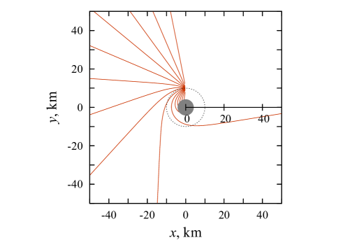
Figure 3: Examples of neutrino trajectories calculated for particles emitted at the distance $10^{6}\,{\rm cm}$ from the Schwarzschild black hole with mass $M=1.4\,M_{\odot}$. Dark grey region illustrates the region surrounded by the Schwarzschild radius $R_{\mathrm{Sch}}(M)$, while the region bounded by the blue dot circle shows the volume within radius of $10^{6}\,{\rm cm}$.

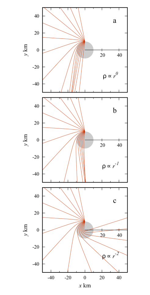
Figure 4: Examples of neutrino trajectories calculated for particles emitted at the NS surface for the case of different mass density distribution inside a compact object: (a) constant mass density, (b) $\rho\propto r^{-1}$, (c) $\rho\propto r^{-2}$. Parameters: $M=1.4\,M_{\odot}$, $R=10^{6}\,{\rm cm}$. For comparison, the same uneven steps for the initial co-latitudes of trajectories were chosen in all three panels.

4.2 Angular distribution of neutrino flux

Utilizing the calculated neutrino trajectories, we derive the angular distribution of neutrino energy flux in the reference frame of a NS (i.e., in a frame where the star does not rotate). In Fig. 5, the angular distribution of the energy flux is presented in units of the isotropic energy flux for cases with internal mass density distributed according to power laws. The angular distributions of neutrino energy flux are contingent upon the structure of the compact object. Trajectories of neutrinos emitted from a specific point on the NS surface are bent towards the diametrically opposite point on the surface, leading to a substantial amplification (by a factor of $>10$) of neutrino energy flux in that direction. In instances of strong mass concentration towards the centre of the compact object, the angular distribution of flux over co-latitude $\theta$ exhibits a peak at $\theta=\pi$ (see Fig. 5c); note that the corresponding convergence of trajectories is not visible in Fig. 4c. For weaker mass concentration towards the centre, the angular distribution of the flux displays a peak at $\theta<\pi$ (see Fig. 5ab and compare with Fig. 4ab). This peak can either be singular (Fig. 5a) or split into two ones at $\theta=\pi$ and $\theta<\pi$ (Fig. 5b). Similar peaks have been reported earlier for photons lensed in the gravitational field of a NS (see Fig. 3, 4 and 9 in Riffert & Meszaros 1988, Fig. 10–12 in Mushtukov et al. 2018a, and Fig. 6 in Mushtukov et al. 2024).

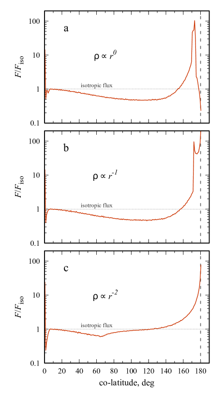
Figure 5: Angular distribution of neutrino energy flux from one of the poles of a compact star is given by red solid line. Horizontal dotted line shows the level of the isotropic neutrino energy flux. Different panels correspond to different mass distribution inside a NS: the mass density (a) $\rho$ is constant, (b) $\rho\propto r^{-1}$, (c) $\rho\propto r^{-2}$.

Angular distributions of the neutrino flux for realistic EoSs are shown in Fig. 6. These distributions differ significantly for the NSs of different masses for a given EoS (compare the red solid and black dotted lines in Fig. 6). The two-peak structure is visible in Figs.  6a and 6b at $M=1.4~{}M_{\odot}$, and it is especially noticeable in all three panels at $M=2~{}M_{\odot}$, when the pairs of peaks are far apart in the co-latitudes.

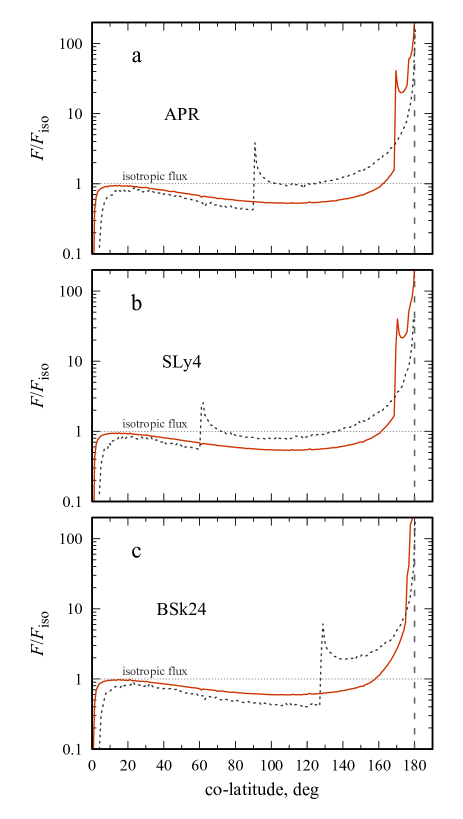
Figure 6: Angular distribution of neutrino energy flux from one of the poles of a NS is given by red solid (black dotted) line for $1.4M_{\odot}$ ($2M_{\odot}$) NS. Horizontal dotted line shows the level of the isotropic neutrino energy flux. Different panels correspond to different equations of state: (a) ARP, (b) SLy4, (c) BSk24. In the case of relatively cold NSs under consideration, neutrino energy does not affect neutrino transfer within a star and, thus, the angular distribution.

In the case of strange stars, unlike the NSs, neutrino absorption can be noticeable. Nevertheless, angular distribution becomes strongly anisotropic and neutrino energy flux can exceed the isotropic flux by more than an order of magnitude (see Fig. 7). Only at high energies $\sim 1\,{\rm MeV}$, some fraction of neutrinos is absorbed, which reduces the flux in the direction opposite to the location of emitting pole of a star (compare solid and dotted lines in Fig. 7).

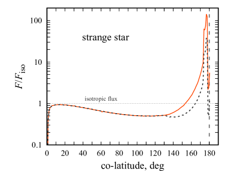
Figure 7: The angular distribution of neutrino energy flux from one of the poles of a strange star with $M=1.4M_{\odot}$ and $M_{r}$ conforming with the EoS proposed by Zdunik (2000). Different lines are calculated for different neutrino energy: $100\,{\rm keV}$ (solid red) and $1\,{\rm MeV}$ (dotted black).

4.3 Luminosity function

Using the calculated angular distributions of neutrino energy flux, we derive theoretical distributions of NSs over the neutrino amplification factor $a_{\nu}$ and calculate the fraction ${\cal F}(a_{\nu})$ of NSs with amplification factors above specific values according to Eq. (23), as described in subsection 3.2. These distributions are shown in Fig. 8.

One can see that the distributions of neutrino pulsars over the amplification factor are relatively restricted: the majority of objects exhibit amplification factors within the interval $a_{\nu}\in(0.5,10)$. The anticipated population of objects with relatively large amplification factors decreases for larger NS masses (see Fig. 8). For the considered EoSs, only $\sim 0.2\%$ ($\sim 0.02\%$) of neutrino pulsars demonstrate an amplification factor $a_{\nu}>10$ for NS masses of $1.4M_{\odot}$ ($2M_{\odot}$). The expected distribution of objects over the amplification factor depends on the EoS insignificantly (compare different lines in Fig. 8).

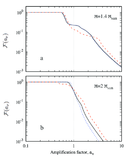
Figure 8: Fraction of neutrino pulsars of amplification factor exceeding $a_{\nu}$. Different lines show results calculated for different EoSs: APR (solid black), SLy4 (dotted blue) and BSk24 (dashed red). Different panels correspond to different masses of a NS: (a) $M=1.4\,M_{\odot}$, (b) $M=2\,M_{\odot}$. One can see that large mass of a NS reduces significantly a fraction of strongly amplified sources.

In the case of strange stars, the distribution of objects over the amplification factor depends on neutrino energy. About $10\%$ of ULX hosting strange stars can demonstrate amplification factor $a_{\nu}>2$ and $\sim 0.2\%$ can show amplification factors $a_{\nu}>10$ (see Fig. 9).

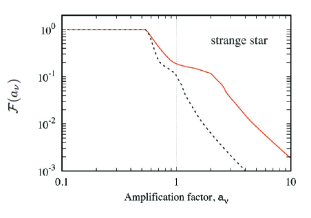
Figure 9: Fraction of neutrino pulsars of amplification factor exceeding $a_{\nu}$ calculated for the case of a strange star with $M=1.4M_{\odot}$ and $M_{r}$ conforming with the EoS proposed by Zdunik (2000). Different lines are calculated for different neutrino energy: $100\,{\rm keV}$ (solid red) and $1\,{\rm MeV}$ (dotted black). The line corresponding to higher neutrino energy shows smaller fractions because of neutrino absorption in a star.

5 Summary

We have explored the impact of gravitational bending on neutrino emission in strongly magnetized NSs undergoing extreme mass accretion rates, such as bright X-ray transients or ULX pulsars. NSs interiors in the considered class objects are cold enough (temperature $\lesssim 10\,{\rm keV}$) to be completely transparent to neutrino emission in keV and MeV energy bands (Haensel & Jerzak, 1987). Thus, a fraction of neutrino emission is going through a NS experiencing gravitational bending. Through Monte Carlo simulations in the metric generated by spherically symmetric and quasi-static mass distribution within a NS, we simulated neutrino beam patterns (Figs. 5, 6, 7) influenced by neutrino gravitational bending. The gravitational bending induces strong anisotropy in neutrino emission within the NS reference frame, leading to the phenomenon of neutrino pulsars.

Using calculated beam patterns, we have obtained the theoretical distributions of neutrino pulsars over the amplification factors (1) that show the ratio of apparent (17) and actual luminosity in neutrinos (see Fig. 8 and 9). These distributions reveal limited ranges of amplification factors. The majority of neutrino pulsars are expected to fall within the interval $a_{\nu}\in(0.5,10)$. For the considered equations of state, only approximately $\sim 0.2\%$ ($\sim 0.02\%$) of neutrino pulsars exhibit an amplification factor $a_{\nu}>10$ at a neutron star mass of $1.4M_{\odot}$ ($2M_{\odot}$). Thus, the expected neutrino flux from known pulsating ULXs and bright Be X-ray transients remain to be below the isotropic neutrino background even in the case of flux amplification due to neutrino gravitational bending (see previous estimations that neglect gravitational bending in Asthana et al. 2023).

In the case of strange stars, where the core of a star is composed of quark matter, high energy neutrinos can be subject to absorption. As a result, neutrino beam pattern becomes energy dependent (see Fig. 7), which affects the expected distribution of objects powered by accretion onto strange start over the amplification factor (see Fig. 9).

Data availability

The calculations presented in this paper were performed using a private code developed and owned by the corresponding author. All the data appearing in the figures are available upon request.

Appendix A Simulations of neutrino trajectories

We calculate neutrino trajectories assuming that they are described by differential equation (16) while the mass distribution is spherically symmetric and given by $M_{r}$. A trajectory is determined by the initial coordinates of a particle $\bm{r}_{0}$ and initial direction of its motion, which is given by the unit vector of particle velocity

$$\bm{e}_{v0}=\frac{\bm{v}_{0}}{|\bm{v}_{0}|}.$$ (24)

Simulating a trajectory, we choose a spacial separation between the nearest two points of approximate trajectory $\Delta s$ and follow the steps:

1. Using the starting point of particle trajectory $\bm{r}_{0}$ and the direction of its initial velocity given by the unit vector $\bm{e}_{v0}$ (24), we calculate the second point of approximate trajectory:

   $$\bm{r}_{1}=\bm{r}_{0}+\bm{e}_{v0}\Delta s.$$ (25)

   At this step $i=1$.

2. Then we get the angle between positions $\bm{r}_{i}$ and $\bm{r}_{i-1}$:

   $$\cos\Delta\varphi_{i,i-1}=\frac{(\bm{r}_{i},\bm{r}_{i-1})}{|\bm{r}_{i}|\,|\bm{r}_{i-1}|},$$ (26)

   where $(\bm{r}_{i},\bm{r}_{i-1})=\sum_{j=1}^{3}r^{(j)}_{i}r^{(j)}_{i-1}$ denotes the scalar productions of two vectors and $r_{i}^{(j)}$ is $j^{\rm th}$ Cartesian coordinate of vector $\bm{r}_{i}$.

3. We get direction towards the $(i+1)^{\rm th}$ point of approximate particle trajectory:

   $$\bm{e}_{r,i+1}=\frac{\bm{r}_{i}+\bm{e}_{v,i-1}\Delta s}{|\bm{r}_{i}+\bm{e}_{v,i-1}\Delta s|}$$ (27)

   and the angle between $\bm{e}_{r,i+1}$ and $\bm{r}_{i}$:

   $$\Delta\varphi_{i+1,i}^{*}=\frac{(\bm{e}_{r,i+1},\bm{r}_{i})}{|\bm{r}_{i}|}.$$ (28)

4. We calculate $u$-functions for the latest two points of trajectory:

   $$u_{i}=0.5R_{\rm Sch}(M_{r_{i}})/r_{i},\quad u_{i-1}=0.5R_{\rm Sch}(M_{r_{i-1}})/r_{i-1}$$

   and get $u$-function for a new point of approximate trajectory:

   $$u_{i+1}=\left(1+\frac{1}{\xi_{i}}\right)u_{i}-\frac{u_{i-1}}{\xi_{i}}+u^{\prime\prime}_{i}\Delta\varphi_{i+1,i}\Delta\varphi_{i,i-1},$$ (29)

   where $\xi_{i}\equiv\Delta\varphi_{i,i-1}/\Delta\varphi_{i+1,i}$ and

   $$u^{\prime\prime}_{i}=3u_{i}^{2}-u_{i}$$ (30)

   according (16).

5. We get an estimation of the radial distance towards a new point of particle trajectory $r_{i+1}\simeq 0.5R_{\rm Sch}(M_{i})/u_{i+1}$ and calculate its position:

   $$\bm{r}^{*}_{i+1}=r_{i+1}\bm{e}_{r,i+1}.$$ (31)

6. Because we want to get trajectory approximated by segments of a fixed length $\Delta s$, we recalculate the position of the latest point of neutrino trajectory as

   $$\bm{r}_{i+1}=\bm{r}_{i}+\frac{\bm{r}^{*}_{i+1}-\bm{r}_{i}}{|\bm{r}^{*}_{i+1}-\bm{r}_{i}|}\Delta s.$$ (32)

   The unit vector of neutrino velocity at the latest segment of trajectory is given by

   $$\bm{e}_{v,i}=\frac{\bm{r}_{i+1}-\bm{r}_{i}}{|\bm{r}_{i+1}-\bm{r}_{i}|}.$$ (33)

7. We stop trajectory simulation if the particle experiences scattering at a given coordinate or if it is far from the central compact object: $|\bm{r}_{i+1}|>5\times 10^{2}R_{\rm Sch}$. In this case, we have a final direction of particle motion given by (33). Otherwise, we return to step 3 and continue the simulation of the trajectory.

To control the accuracy of trajectory calculations, we perform it for smaller spacial step $\Delta s_{1}=0.5\,\Delta s$. In the case of similar results of the simulation, we stop the improvement of accuracy.

The results of the performed algorithm were verified by comparison of its results with the results of algorithms applied earlier in Mushtukov et al. 2018a; Mushtukov et al. 2024 to trace photon trajectories in X-ray pulsars.

References

- Akmal et al. (1998) Akmal A., Pandharipande V. R., Ravenhall D. G., 1998, Phys. Rev. C, 58, 1804
- Alcock et al. (1986) Alcock C., Farhi E., Olinto A., 1986, ApJ, 310, 261
- Antoniadis et al. (2013) Antoniadis J., et al., 2013, Science, 340, 448
- Asthana et al. (2023) Asthana A., Mushtukov A. A., Dobrynina A. A., Ognev I. S., 2023, MNRAS, 522, 3405
- Bachetti et al. (2014) Bachetti M., et al., 2014, Nature, 514, 202
- Basko & Sunyaev (1975) Basko M. M., Sunyaev R. A., 1975, A&A, 42, 311
- Blinnikov et al. (2022) Blinnikov S., Yudin A., Kramarev N., Potashov M., 2022, Particles, 5, 198
- Doroshenko et al. (2022) Doroshenko V., et al., 2022, Nature Astronomy, 6, 1433
- Doroshenko et al. (2023) Doroshenko V., et al., 2023, A&A, 677, A57
- Douchin & Haensel (2001) Douchin F., Haensel P., 2001, A&A, 380, 151
- Fabrika et al. (2021) Fabrika S. N., Atapin K. E., Vinokurov A. S., Sholukhova O. N., 2021, Astrophysical Bulletin, 76, 6
- González-Caniulef et al. (2019) González-Caniulef D., Guillot S., Reisenegger A., 2019, MNRAS, 490, 5848
- Haensel & Jerzak (1987) Haensel P., Jerzak A. J., 1987, A&A, 179, 127
- Haensel & Potekhin (2004) Haensel P., Potekhin A. Y., 2004, A&A, 428, 191
- Haensel et al. (1986) Haensel P., Zdunik J. L., Schaefer R., 1986, A&A, 160, 121
- Haensel et al. (2007) Haensel P., Potekhin A. Y., Yakovlev D. G., 2007, Neutron Stars 1 : Equation of State and Structure. Astrophysics and Space Science Library Vol. 326, Springer, New York
- Harding & Lai (2006) Harding A. K., Lai D., 2006, Reports on Progress in Physics, 69, 2631
- Heyl et al. (2023) Heyl J., et al., 2023, arXiv e-prints, p. arXiv:2311.03667
- Horowitz et al. (2020) Horowitz C. J., Piekarewicz J., Reed B., 2020, Phys. Rev. C, 102, 044321
- Israel et al. (2017) Israel G. L., et al., 2017, Science, 355, 817
- Kaminker et al. (1992) Kaminker A. D., Levenfish K. P., Yakovlev D. G., Amsterdamski P., Haensel P., 1992, Phys. Rev. D, 46, 3256
- King et al. (2017) King A., Lasota J.-P., Kluźniak W., 2017, MNRAS, 468, L59
- Malacaria et al. (2023) Malacaria C., et al., 2023, A&A, 675, A29
- Markozov & Mushtukov (2024) Markozov I. D., Mushtukov A. A., 2024, MNRAS, 527, 5374
- Miller et al. (2019) Miller M. C., et al., 2019, ApJ, 887, L24
- Miller et al. (2021) Miller M. C., et al., 2021, ApJ, 918, L28
- Misner et al. (1973) Misner C. W., Thorne K. S., Wheeler J. A., 1973, Gravitation. Freeman and Co., New York
- Mönkkönen et al. (2022) Mönkkönen J., Tsygankov S. S., Mushtukov A. A., Doroshenko V., Suleimanov V. F., Poutanen J., 2022, MNRAS, 515, 571
- Mushtukov & Portegies Zwart (2023) Mushtukov A. A., Portegies Zwart S., 2023, MNRAS, 518, 5457
- Mushtukov & Tsygankov (2022) Mushtukov A., Tsygankov S., 2022, arXiv e-prints, p. arXiv:2204.14185
- Mushtukov et al. (2015) Mushtukov A. A., Suleimanov V. F., Tsygankov S. S., Poutanen J., 2015, MNRAS, 454, 2539
- Mushtukov et al. (2018a) Mushtukov A. A., Verhagen P. A., Tsygankov S. S., van der Klis M., Lutovinov A. A., Larchenkova T. I., 2018a, MNRAS, 474, 5425
- Mushtukov et al. (2018b) Mushtukov A. A., Tsygankov S. S., Suleimanov V. F., Poutanen J., 2018b, MNRAS, 476, 2867
- Mushtukov et al. (2019) Mushtukov A. A., Ognev I. S., Nagirner D. I., 2019, MNRAS, 485, L131
- Mushtukov et al. (2021) Mushtukov A. A., Portegies Zwart S., Tsygankov S. S., Nagirner D. I., Poutanen J., 2021, MNRAS, 501, 2424
- Mushtukov et al. (2023) Mushtukov A. A., et al., 2023, MNRAS, 524, 2004
- Mushtukov et al. (2024) Mushtukov A. A., Weng A., Tsygankov S. S., Mereminskiy I. A., 2024, MNRAS, 530, 3051
- Nättilä et al. (2017) Nättilä J., Miller M. C., Steiner A. W., Kajava J. J. E., Suleimanov V. F., Poutanen J., 2017, A&A, 608, A31
- Pal & Dutt-Mazumder (2011) Pal K., Dutt-Mazumder A. K., 2011, Phys. Rev. D, 84, 034004
- Pearson et al. (2018) Pearson J. M., Chamel N., Potekhin A. Y., Fantina A. F., Ducoin C., Dutta A. K., Goriely S., 2018, MNRAS, 481, 2994
- Postnov et al. (2013) Postnov K., Shakura N., Staubert R., Kochetkova A., Klochkov D., Wilms J., 2013, MNRAS, 435, 1147
- Potekhin & Chabrier (2018) Potekhin A. Y., Chabrier G., 2018, A&A, 609, A74
- Potekhin et al. (2020) Potekhin A. Y., Zyuzin D. A., Yakovlev D. G., Beznogov M. V., Shibanov Y. A., 2020, MNRAS, 496, 5052
- Rezzolla et al. (2018) Rezzolla L., Most E. R., Weih L. R., 2018, ApJ, 852, L25
- Richardson et al. (1979) Richardson M. B., van Horn H. M., Savedoff M. P., 1979, ApJS, 39, 29
- Riffert & Meszaros (1988) Riffert H., Meszaros P., 1988, ApJ, 325, 207
- Romani et al. (2021) Romani R. W., Kandel D., Filippenko A. V., Brink T. G., Zheng W., 2021, ApJ, 908, L46
- Romani et al. (2022) Romani R. W., Kandel D., Filippenko A. V., Brink T. G., Zheng W., 2022, ApJ, 934, L17
- Sawyer & Soni (1979) Sawyer R. F., Soni A., 1979, ApJ, 230, 859
- Schäfer & Schwenzer (2004) Schäfer T., Schwenzer K., 2004, Phys. Rev. D, 70, 114037
- Shapiro & Teukolsky (1983) Shapiro S. L., Teukolsky S. A., 1983, Black holes, white dwarfs, and neutron stars: The physics of compact objects. Wiley, New York, doi:10.1002/9783527617661
- Tanashkin et al. (2022) Tanashkin A. S., Karpova A. V., Potekhin A. Y., Shibanov Y. A., Zyuzin D. A., 2022, MNRAS, 516, 13
- Thorne (1977) Thorne K. S., 1977, ApJ, 212, 825
- Tsygankov et al. (2017) Tsygankov S. S., Doroshenko V., Lutovinov A. A., Mushtukov A. A., Poutanen J., 2017, A&A, 605, A39
- Tsygankov et al. (2022) Tsygankov S. S., et al., 2022, ApJ, 941, L14
- Tsygankov et al. (2023) Tsygankov S. S., et al., 2023, A&A, 675, A48
- Vantournhout et al. (2006) Vantournhout K., Jachovicz N., Ryckebusch J., 2006, in Mengoni A., et al., eds, International Symposium on Nuclear Astrophysics – Nuclei in the Cosmos. p. 240.1, doi:10.22323/1.028.0240
- Verbiest et al. (2008) Verbiest J. P. W., et al., 2008, ApJ, 679, 675
- Vinciguerra et al. (2024) Vinciguerra S., et al., 2024, ApJ, 961, 62
- Wang & Frank (1981) Wang Y. M., Frank J., 1981, A&A, 93, 255
- Witten (1984) Witten E., 1984, Phys. Rev. D, 30, 272
- Yakovlev et al. (2005) Yakovlev D. G., Gnedin O. Y., Gusakov M. E., Kaminker A. D., Levenfish K. P., Potekhin A. Y., 2005, Nuclear Phys. A, 752, 590
- Zdunik (2000) Zdunik J. L., 2000, A&A, 359, 311
- Zhang et al. (2022) Zhang L., Blaes O., Jiang Y.-F., 2022, MNRAS, 515, 4371