Schmidt modes carrying orbital angular momentum generated by cascaded systems pumped with Laguerre-Gaussian beams

D. Scharwald    L. Gehse    P. R. Sharapova Department of Physics, Paderborn University, Warburger Straße 100, 33098 Paderborn, Germany
Abstract

Orbital Angular Momentum (OAM) modes are an important resource used in various branches of quantum science and technology due to their unique helical structure and countably infinite basis. Generating light that simultaneously carries high-order orbital angular momenta and exhibits quantum correlations is a challenging task. In this work, we present a theoretical approach to the generation of correlated Schmidt modes carrying OAM via parametric down-conversion (PDC) in cascaded nonlinear systems (nonlinear interferometers) pumped by Laguerre-Gaussian beams. We demonstrate how the number of generated modes and their population can be controlled by varying the pump parameters, the gain of the PDC process and the distance between the crystals. We investigate the angular displacement sensitivity of these interferometers and demonstrate that it can overcome the classical shot noise limit.

I INTRODUCTION

Structured light has been studied extensively over the past decade and currently plays an important role in various areas of physics [1]. One important type of structured light is light that carries orbital angular momentum (OAM) [2, 3]. These beams have a helical azimuthal phase dependency $\mathrm{e}^{-\mathrm{i}l\varphi}$ with a central singularity, where $\varphi$ is the azimuthal angle and $l\in\mathbb{Z}$ the OAM quantum number (topological charge number) of the mode [1, 3, 4]. Due to their unique helical structure and countably infinite basis, OAM modes are an important resource for quantum communication, quantum computing, quantum information processing [5, 6] and quantum cryptography [7]. They can be generated using spatial light modulators [8], plasmonic nanostructures [9] or in parametric down-conversion [10, 11, 12, 6] (PDC) and four-wave mixing [13] (FWM) processes and can be transmitted using multimode fibers [14, 4]. Recently, the transmission of OAM modes and their superpositions over long distances has been demonstrated [15], which is an important element for the creation of free-space optical communication links [16]. In addition to the applications mentioned above, OAM modes play an important role in metrology: It has been shown that entangled OAM states can be used to improve the angular displacement sensitivity [8, 17, 18] by a factor of $1/l$.

Thus, the generation and manipulation of correlated light carrying high-order orbital angular momenta is a vital problem. Cascaded systems of PDC processes, in particular nonlinear interferometers, constitute an important tool that can be used for these purposes since they make it possible to manipulate the set of populated OAM modes [11, 19]. Additionally, nonlinear interferometers have taken an important role in quantum metrology as they can be used to overcome the shot noise level for the phase sensitivity, which is the limit of any classical interferometer [20, 21, 22].

In this work, we present a theoretical framework to describe PDC and nonlinear interferometers pumped by Laguerre-Gaussian beams. Our framework is based on the Schmidt-mode formalism developed in Ref. 11 and provides valuable analytical insights that would otherwise not be possible with rigorous methods, such as the integro-differential equations approach [23], that include time-ordering effects and can in general only be evaluated numerically.

Baghdasaryan et al. [24] have also investigated PDC with Laguerre-Gaussian pump beams to analyze the role of the Gouy phase in SPDC. For this, the SPDC state is expanded over Laguerre-Gaussian modes for the signal and idler beams. However, outside of the double-Gaussian approximation, the Schmidt modes of PDC are generally not exactly given by Laguerre-Gaussian modes [10, 11] and only look comparatively similar. Therefore, in Sec. II, we start by explicitly evaluating the spatial integral of the PDC-Hamiltonian and arrive at the two-photon amplitude (TPA) and the Schmidt decomposition for PDC with a Laguerre-Gaussian pump beam. Along the way, we will highlight similarities and differences that arise compared to the case of Gaussian pump [11] and illustrate the conservation of angular momentum [22]. Furthermore, since we present a general derivation allowing for arbitrary OAM and radial indices of the pump beam, our work can serve as a starting point for a theoretical framework with arbitrarily shaped pump beams (pump engineering), since a given pump field can always be expanded in terms of the OAM modes [24]. This work may also provide the basis for future work on the description of PDC with Laguerre-Gaussian pump beams using the integro-differential equations approach [23].

Next, in Sec. III, we investigate the modal structure of the PDC radiation generated by pumping nonlinear interferometers with Laguerre-Gaussian beams with different OAM and radial numbers. To this end, we analyze the distribution of the weights (Schmidt eigenvalues) of the generated Schmidt modes and the output intensity profiles. In Sec. IV, we investigate the angular displacement sensitivity of these interferometers. Finally, we draw our conclusion in Sec. V.

II THEORETICAL MODEL

II.1 The PDC Hamiltonian for Laguerre-Gaussian pump beams

In its general form, the Hamiltonian describing the parametric down-conversion (PDC) process is given by [11, 25, 26]:

$\displaystyle\hat{H}$ $\displaystyle\!\propto\!\int\!\mathrm{d}^{3}r\,\chi^{\left(2\right)}\mathchoice{\!\left({\boldsymbol{r}}\right)}{\!\left({\boldsymbol{r}}\right)}{\left({\boldsymbol{r}}\right)}{\left({\boldsymbol{r}}\right)}\hat{E}_{p}^{\left(+\right)}\mathchoice{\!\left({\boldsymbol{r},t}\right)}{\!\left({\boldsymbol{r},t}\right)}{\left({\boldsymbol{r},t}\right)}{\left({\boldsymbol{r},t}\right)}\hat{E}_{s}^{\left(-\right)}\mathchoice{\!\left({\boldsymbol{r},t}\right)}{\!\left({\boldsymbol{r},t}\right)}{\left({\boldsymbol{r},t}\right)}{\left({\boldsymbol{r},t}\right)}\hat{E}_{i}^{\left(-\right)}\mathchoice{\!\left({\boldsymbol{r},t}\right)}{\!\left({\boldsymbol{r},t}\right)}{\left({\boldsymbol{r},t}\right)}{\left({\boldsymbol{r},t}\right)}+\mathrm{h.c.},$ (2.1)

where $\chi^{\left(2\right)}$ is the second order (nonlinear) susceptibility of the PDC section and $\hat{E}_{j}\mathchoice{\!\left({\boldsymbol{r},t}\right)}{\!\left({\boldsymbol{r},t}\right)}{\left({\boldsymbol{r},t}\right)}{\left({\boldsymbol{r},t}\right)}$ are the electric field operators, while the labels $j=p,s,i$ refer to the pump, signal and idler fields, respectively. In the following, we will assume $\chi^{\left(2\right)}$ to be independent of the position space coordinate vector ${\boldsymbol{r}={{\begin{bmatrix}{x}&{y}&{z}\end{bmatrix}}}^{\mathrm{T}}}$. Furthermore, in this work, we restrict ourselves to monochromatic signal and idler fields, so that their field operators can be written as [25]:

$\displaystyle\hat{E}_{j}^{\left(-\right)}\mathchoice{\!\left({\boldsymbol{r},t}\right)}{\!\left({\boldsymbol{r},t}\right)}{\left({\boldsymbol{r},t}\right)}{\left({\boldsymbol{r},t}\right)}$ $\displaystyle=\epsilon_{j}\int\!\mathrm{d}^{2}q_{j}\,\mathrm{e}^{-\mathrm{i}\left[\boldsymbol{q}_{j}\cdot\boldsymbol{r}_{\perp}+k_{j,z}\mathchoice{\!\left({\boldsymbol{q}_{j},\omega_{j}}\right)}{\!\left({\boldsymbol{q}_{j},\omega_{j}}\right)}{\left({\boldsymbol{q}_{j},\omega_{j}}\right)}{\left({\boldsymbol{q}_{j},\omega_{j}}\right)}z-\omega_{j}t\right]}\hat{a}^{\dagger}_{j}\mathchoice{\!\left({\boldsymbol{k}_{j}}\right)}{\!\left({\boldsymbol{k}_{j}}\right)}{\left({\boldsymbol{k}_{j}}\right)}{\left({\boldsymbol{k}_{j}}\right)},$ (2.2)

where $\epsilon_{j}$ is a normalization constant, $j=s,i$, and the transverse wave vector and the transverse coordinate vector are given by $\boldsymbol{q}_{j}={{\begin{bmatrix}{k_{j,x}}&{k_{j,y}}\end{bmatrix}}}^{\mathrm{T}}$ and $\boldsymbol{r}_{\perp}={{\begin{bmatrix}{x}&{y}\end{bmatrix}}}^{\mathrm{T}}$, respectively. Importantly, note that there are only two integrals over the transverse wave vectors and no integral over the frequencies $\omega_{j}$. As a consequence, $k_{j,z}$ is fixed and can be written as a function of $\boldsymbol{q}_{j}$ and $\omega_{j}$, as indicated above.

The pump is described by a strong classical field with a transverse Laguerre-Gaussian profile, so that [3, 13, 27]

$\displaystyle\begin{split}E_{p}^{\left(+\right)}\mathchoice{\!\left({\boldsymbol{r},t}\right)}{\!\left({\boldsymbol{r},t}\right)}{\left({\boldsymbol{r},t}\right)}{\left({\boldsymbol{r},t}\right)}&=E_{0}\frac{r_{\perp}^{{\mathchoice{{\kern 0.29167pt}}{}{}{}|}l_{p}{|\mathchoice{{\kern 0.29167pt}}{}{}{}}}}{w_{0}^{{\mathchoice{{\kern 0.29167pt}}{}{}{}|}l_{p}{|\mathchoice{{\kern 0.29167pt}}{}{}{}}+1}}L^{{\mathchoice{{\kern 0.29167pt}}{}{}{}|}l_{p}{|\mathchoice{{\kern 0.29167pt}}{}{}{}}}_{m_{p}}\mathchoice{\!\left({\frac{2r_{\perp}^{2}}{w_{0}^{2}}}\right)}{\!\left({\frac{2r_{\perp}^{2}}{w_{0}^{2}}}\right)}{\left({\frac{2r_{\perp}^{2}}{w_{0}^{2}}}\right)}{\left({\frac{2r_{\perp}^{2}}{w_{0}^{2}}}\right)}\mathrm{e}^{-\left(\frac{r_{\perp}}{w_{0}}\right)^{2}}\\ &\qquad\times\mathrm{e}^{-\mathrm{i}l_{p}\varphi}\mathrm{e}^{\mathrm{i}\left(\boldsymbol{k}_{p}\cdot\boldsymbol{r}-\omega_{p}t\right)},\end{split}$ (2.3)

where $r_{\perp}={\mathchoice{{\kern 0.41667pt}}{}{}{}|}\boldsymbol{r}_{\perp}{|\mathchoice{{\kern 0.41667pt}}{}{}{}}=\sqrt{x^{2}+y^{2}}$ and $\varphi=\operatorname{arctan2}\mathchoice{\!\left({y,x}\right)}{\!\left({y,x}\right)}{\left({y,x}\right)}{\left({y,x}\right)}$ is111Throughout this work, we will use the two-argument arctangent function $\operatorname{arctan2}$ for clarity, when appropriate. the azimuthal angle in coordinate space. $L^{{\mathchoice{{\kern 0.29167pt}}{}{}{}|}l_{p}{|\mathchoice{{\kern 0.29167pt}}{}{}{}}}_{m_{p}}$ denotes the Laguerre polynomials, so that $l_{p}\in\mathbb{Z}$ and $m_{p}\in\mathbb{N}_{0}$ are the OAM and radial quantum number of the Laguerre-Gaussian pump profile, respectively. $w_{0}$ is the width of the Gaussian term so that the full width at half maximum (FWHM) of the intensity distribution is given by $w_{0}\sqrt{2\ln{2}}$. More specifically, $w_{0}$ can be understood as the $1/\mathrm{e}^{2}$-radius of the intensity distribution of the Gaussian term. We have therefore also assumed that the beam waist diameter is constant over the setup under consideration. This is usually satisfied if the PDC sections are sufficiently thin.

After plugging Eqs. 2.2 and 2.3 into Eq. 2.1 and assuming perfect frequency matching $\omega_{p}=\omega_{s}+\omega_{i}$ (neglecting time-ordering effects), the Hamiltonian can be written in the form

$\displaystyle\hat{H}$ $\displaystyle=\mathrm{i}\hbar\Gamma\iint\!\mathrm{d}^{2}q_{s}\mathrm{d}^{2}q_{i}\,F\mathchoice{\!\left({\boldsymbol{q}_{s},\boldsymbol{q}_{i}}\right)}{\!\left({\boldsymbol{q}_{s},\boldsymbol{q}_{i}}\right)}{\left({\boldsymbol{q}_{s},\boldsymbol{q}_{i}}\right)}{\left({\boldsymbol{q}_{s},\boldsymbol{q}_{i}}\right)}\hat{a}^{\dagger}_{s}\mathchoice{\!\left({\boldsymbol{q}_{s}}\right)}{\!\left({\boldsymbol{q}_{s}}\right)}{\left({\boldsymbol{q}_{s}}\right)}{\left({\boldsymbol{q}_{s}}\right)}\hat{a}^{\dagger}_{i}\mathchoice{\!\left({\boldsymbol{q}_{i}}\right)}{\!\left({\boldsymbol{q}_{i}}\right)}{\left({\boldsymbol{q}_{i}}\right)}{\left({\boldsymbol{q}_{i}}\right)}+\mathrm{h.c.}$ (2.4a)
where
$\displaystyle F\mathchoice{\!\left({\boldsymbol{q}_{s},\boldsymbol{q}_{i}}\right)}{\!\left({\boldsymbol{q}_{s},\boldsymbol{q}_{i}}\right)}{\left({\boldsymbol{q}_{s},\boldsymbol{q}_{i}}\right)}{\left({\boldsymbol{q}_{s},\boldsymbol{q}_{i}}\right)}$ $\displaystyle=Cg_{xy}\mathchoice{\!\left({\boldsymbol{q}_{s},\boldsymbol{q}_{i}}\right)}{\!\left({\boldsymbol{q}_{s},\boldsymbol{q}_{i}}\right)}{\left({\boldsymbol{q}_{s},\boldsymbol{q}_{i}}\right)}{\left({\boldsymbol{q}_{s},\boldsymbol{q}_{i}}\right)}g_{z}\mathchoice{\!\left({\boldsymbol{q}_{s},\boldsymbol{q}_{i}}\right)}{\!\left({\boldsymbol{q}_{s},\boldsymbol{q}_{i}}\right)}{\left({\boldsymbol{q}_{s},\boldsymbol{q}_{i}}\right)}{\left({\boldsymbol{q}_{s},\boldsymbol{q}_{i}}\right)}$ (2.4b)

is the two-photon amplitude (TPA) of the PDC process and $C>0$ is an $l_{p}$- and $m_{p}$-dependent normalization constant to ensure that the TPA is normalized to unity: ${\iint\!\mathrm{d}^{2}q_{s}\mathrm{d}^{2}q_{i}\,{\mathchoice{{\kern 0.41667pt}}{}{}{}|}F\mathchoice{\!\left({\boldsymbol{q}_{s},\boldsymbol{q}_{i}}\right)}{\!\left({\boldsymbol{q}_{s},\boldsymbol{q}_{i}}\right)}{\left({\boldsymbol{q}_{s},\boldsymbol{q}_{i}}\right)}{\left({\boldsymbol{q}_{s},\boldsymbol{q}_{i}}\right)}{|\mathchoice{{\kern 0.41667pt}}{}{}{}}^{2}=1}$. The newly introduced constant $\Gamma=\varepsilon_{0}\frac{\chi^{\left(2\right)}}{3}\frac{1}{C}\epsilon_{s}\epsilon_{i}E_{0}$ is the theoretical gain parameter. We have factorized the TPA so that the function $g_{xy}$ contains the spatial integrals over the (transverse) $xy$-plane and $g_{z}$ contains the integral along the $z$-axis, both of which originate from the PDC Hamiltonian in Eq. 2.1.

II.2 Evaluation of the transverse spatial integral

The integral over the $xy$-plane of the nonlinear medium corresponds to the Fourier transform of the Laguerre-Gaussian envelope. In polar coordinates, $\boldsymbol{q}_{j}\equiv\left(q_{j},\phi_{j}\right)$ (with $j=s,i$) and $\boldsymbol{r}_{\perp}\equiv\left(r,\varphi\right)$, this integral takes the form:

$\displaystyle g_{xy}\mathchoice{\!\left({q_{s},q_{i},\phi_{s},\phi_{i}}\right)}{\!\left({q_{s},q_{i},\phi_{s},\phi_{i}}\right)}{\left({q_{s},q_{i},\phi_{s},\phi_{i}}\right)}{\left({q_{s},q_{i},\phi_{s},\phi_{i}}\right)}$ $\displaystyle=\int\!\mathrm{d}r\int\!\mathrm{d}\varphi\,\left(\frac{r}{w_{0}}\right)^{{\mathchoice{{\kern 0.29167pt}}{}{}{}|}l_{p}{|\mathchoice{{\kern 0.29167pt}}{}{}{}}+1}L^{{\mathchoice{{\kern 0.29167pt}}{}{}{}|}l_{p}{|\mathchoice{{\kern 0.29167pt}}{}{}{}}}_{m_{p}}\mathchoice{\!\left({\frac{2r^{2}}{w_{0}^{2}}}\right)}{\!\left({\frac{2r^{2}}{w_{0}^{2}}}\right)}{\left({\frac{2r^{2}}{w_{0}^{2}}}\right)}{\left({\frac{2r^{2}}{w_{0}^{2}}}\right)}\mathrm{e}^{-\left(\frac{r}{w_{0}}\right)^{2}}\mathrm{e}^{-\mathrm{i}l_{p}\varphi}\mathrm{e}^{-\mathrm{i}r\left[q_{s}\cos\left(\varphi-\phi_{s}\right)+q_{i}\cos\left(\varphi-\phi_{i}\right)\right]}.$ (2.5)

Since the last exponent is a superposition of weighted cosine terms, it can be rewritten in terms of a single sine function [28], p. 84:

$\displaystyle q_{s}\cos\mathchoice{\!\left({\varphi-\phi_{s}}\right)}{\!\left({\varphi-\phi_{s}}\right)}{\left({\varphi-\phi_{s}}\right)}{\left({\varphi-\phi_{s}}\right)}+q_{i}\cos\mathchoice{\!\left({\varphi-\phi_{i}}\right)}{\!\left({\varphi-\phi_{i}}\right)}{\left({\varphi-\phi_{i}}\right)}{\left({\varphi-\phi_{i}}\right)}=\xi\mathchoice{\!\left({q_{s},q_{i},\phi_{s},\phi_{i}}\right)}{\!\left({q_{s},q_{i},\phi_{s},\phi_{i}}\right)}{\left({q_{s},q_{i},\phi_{s},\phi_{i}}\right)}{\left({q_{s},q_{i},\phi_{s},\phi_{i}}\right)}\sin\mathchoice{\!\left[{\varphi+\psi\mathchoice{\!\left({q_{s},q_{i},\phi_{s},\phi_{i}}\right)}{\!\left({q_{s},q_{i},\phi_{s},\phi_{i}}\right)}{\left({q_{s},q_{i},\phi_{s},\phi_{i}}\right)}{\left({q_{s},q_{i},\phi_{s},\phi_{i}}\right)}}\right]}{\!\left[{\varphi+\psi\mathchoice{\!\left({q_{s},q_{i},\phi_{s},\phi_{i}}\right)}{\!\left({q_{s},q_{i},\phi_{s},\phi_{i}}\right)}{\left({q_{s},q_{i},\phi_{s},\phi_{i}}\right)}{\left({q_{s},q_{i},\phi_{s},\phi_{i}}\right)}}\right]}{\left[{\varphi+\psi\mathchoice{\!\left({q_{s},q_{i},\phi_{s},\phi_{i}}\right)}{\!\left({q_{s},q_{i},\phi_{s},\phi_{i}}\right)}{\left({q_{s},q_{i},\phi_{s},\phi_{i}}\right)}{\left({q_{s},q_{i},\phi_{s},\phi_{i}}\right)}}\right]}{\left[{\varphi+\psi\mathchoice{\!\left({q_{s},q_{i},\phi_{s},\phi_{i}}\right)}{\!\left({q_{s},q_{i},\phi_{s},\phi_{i}}\right)}{\left({q_{s},q_{i},\phi_{s},\phi_{i}}\right)}{\left({q_{s},q_{i},\phi_{s},\phi_{i}}\right)}}\right]},$ (2.6a)
where
$\displaystyle\xi\mathchoice{\!\left({q_{s},q_{i},\phi_{s},\phi_{i}}\right)}{\!\left({q_{s},q_{i},\phi_{s},\phi_{i}}\right)}{\left({q_{s},q_{i},\phi_{s},\phi_{i}}\right)}{\left({q_{s},q_{i},\phi_{s},\phi_{i}}\right)}=\sqrt{q_{s}^{2}+q_{i}^{2}+2q_{s}q_{i}\cos\mathchoice{\!\left({\phi_{s}-\phi_{i}}\right)}{\!\left({\phi_{s}-\phi_{i}}\right)}{\left({\phi_{s}-\phi_{i}}\right)}{\left({\phi_{s}-\phi_{i}}\right)}},$ (2.6b)
$\displaystyle\psi\mathchoice{\!\left({q_{s},q_{i},\phi_{s},\phi_{i}}\right)}{\!\left({q_{s},q_{i},\phi_{s},\phi_{i}}\right)}{\left({q_{s},q_{i},\phi_{s},\phi_{i}}\right)}{\left({q_{s},q_{i},\phi_{s},\phi_{i}}\right)}=\operatorname{arctan2}\mathchoice{\!\left({q_{s}\cos\phi_{s}+q_{i}\cos\phi_{i},q_{s}\sin\phi_{s}+q_{i}\sin\phi_{i}}\right)}{\!\left({q_{s}\cos\phi_{s}+q_{i}\cos\phi_{i},q_{s}\sin\phi_{s}+q_{i}\sin\phi_{i}}\right)}{\left({q_{s}\cos\phi_{s}+q_{i}\cos\phi_{i},q_{s}\sin\phi_{s}+q_{i}\sin\phi_{i}}\right)}{\left({q_{s}\cos\phi_{s}+q_{i}\cos\phi_{i},q_{s}\sin\phi_{s}+q_{i}\sin\phi_{i}}\right)}.$ (2.6c)

Note that $\xi={\mathchoice{{\kern 0.41667pt}}{}{}{}|}\boldsymbol{q}_{p}{|\mathchoice{{\kern 0.41667pt}}{}{}{}}$ [24]. The transverse integral can then be rewritten in a more simple form:

$\displaystyle g_{xy}\mathchoice{\!\left({q_{s},q_{i},\phi_{s},\phi_{i}}\right)}{\!\left({q_{s},q_{i},\phi_{s},\phi_{i}}\right)}{\left({q_{s},q_{i},\phi_{s},\phi_{i}}\right)}{\left({q_{s},q_{i},\phi_{s},\phi_{i}}\right)}$ $\displaystyle=\int\!\mathrm{d}r\,\left(\frac{r}{w_{0}}\right)^{{\mathchoice{{\kern 0.29167pt}}{}{}{}|}l_{p}{|\mathchoice{{\kern 0.29167pt}}{}{}{}}+1}L^{{\mathchoice{{\kern 0.29167pt}}{}{}{}|}l_{p}{|\mathchoice{{\kern 0.29167pt}}{}{}{}}}_{m_{p}}\mathchoice{\!\left({\frac{2r^{2}}{w_{0}^{2}}}\right)}{\!\left({\frac{2r^{2}}{w_{0}^{2}}}\right)}{\left({\frac{2r^{2}}{w_{0}^{2}}}\right)}{\left({\frac{2r^{2}}{w_{0}^{2}}}\right)}\mathrm{e}^{-\left(\frac{r}{w_{0}}\right)^{2}}\int_{0}^{2\pi}\!\mathrm{d}\varphi\,\mathrm{e}^{\mathrm{i}\left(-r\xi\sin\mathchoice{\!\left({\varphi+\psi}\right)}{\!\left({\varphi+\psi}\right)}{\left({\varphi+\psi}\right)}{\left({\varphi+\psi}\right)}-l_{p}\varphi\right)}.$ (2.7)

The integration over the polar angle $\varphi$ can be performed by using the definition of the Bessel functions of the first kind $J_{n}$ [24];[29], p. 20 and can be evaluated as:

$\displaystyle\begin{split}&\int_{0}^{2\pi}\!\mathrm{d}\varphi\,\mathrm{e}^{\mathrm{i}\left(-r\xi\sin\mathchoice{\!\left({\varphi+\psi}\right)}{\!\left({\varphi+\psi}\right)}{\left({\varphi+\psi}\right)}{\left({\varphi+\psi}\right)}-l_{p}\varphi\right)}=2\pi\left[-\operatorname{sgn}\mathchoice{\!\left({l_{p}}\right)}{\!\left({l_{p}}\right)}{\left({l_{p}}\right)}{\left({l_{p}}\right)}\right]^{l_{p}}\mathrm{e}^{\mathrm{i}l_{p}\psi}J_{{\mathchoice{{\kern 0.29167pt}}{}{}{}|}l_{p}{|\mathchoice{{\kern 0.29167pt}}{}{}{}}}\mathchoice{\!\left({r\xi}\right)}{\!\left({r\xi}\right)}{\left({r\xi}\right)}{\left({r\xi}\right)},\end{split}$ (2.8)

where $\operatorname{sgn}$ is the sign function. The remaining integral over the radial coordinate $r$ then becomes a Hankel transformation integral of order ${\mathchoice{{\kern 0.41667pt}}{}{}{}|}l_{p}{|\mathchoice{{\kern 0.41667pt}}{}{}{}}$ [28], p. 768:

$\displaystyle g_{xy}\mathchoice{\!\left({q_{s},q_{i},\phi_{s},\phi_{i}}\right)}{\!\left({q_{s},q_{i},\phi_{s},\phi_{i}}\right)}{\left({q_{s},q_{i},\phi_{s},\phi_{i}}\right)}{\left({q_{s},q_{i},\phi_{s},\phi_{i}}\right)}$ $\displaystyle=2\pi\left[-\operatorname{sgn}\mathchoice{\!\left({l_{p}}\right)}{\!\left({l_{p}}\right)}{\left({l_{p}}\right)}{\left({l_{p}}\right)}\right]^{l_{p}}\mathrm{e}^{\mathrm{i}l_{p}\psi}\int_{0}^{\infty}\!\mathrm{d}r\,\left(\frac{r}{w_{0}}\right)^{{\mathchoice{{\kern 0.29167pt}}{}{}{}|}l_{p}{|\mathchoice{{\kern 0.29167pt}}{}{}{}}+1}L^{{\mathchoice{{\kern 0.29167pt}}{}{}{}|}l_{p}{|\mathchoice{{\kern 0.29167pt}}{}{}{}}}_{m_{p}}\mathchoice{\!\left({\frac{2r^{2}}{w_{0}^{2}}}\right)}{\!\left({\frac{2r^{2}}{w_{0}^{2}}}\right)}{\left({\frac{2r^{2}}{w_{0}^{2}}}\right)}{\left({\frac{2r^{2}}{w_{0}^{2}}}\right)}\mathrm{e}^{-\left(\frac{r}{w_{0}}\right)^{2}}J_{{\mathchoice{{\kern 0.29167pt}}{}{}{}|}l_{p}{|\mathchoice{{\kern 0.29167pt}}{}{}{}}}\mathchoice{\!\left({r\xi}\right)}{\!\left({r\xi}\right)}{\left({r\xi}\right)}{\left({r\xi}\right)}.$ (2.9)

Substituting $x=\sqrt{2}r/w_{0}$, this integral can be directly evaluated using the following Hankel transform integral formula [30], p. 42:

$\displaystyle\begin{split}\int_{0}^{\infty}\!\mathrm{d}x\,x^{\nu+\frac{1}{2}}\mathrm{e}^{-\frac{1}{2}x^{2}}L^{\nu}_{n}\mathchoice{\!\left({x^{2}}\right)}{\!\left({x^{2}}\right)}{\left({x^{2}}\right)}{\left({x^{2}}\right)}J_{\nu}\mathchoice{\!\left({xy}\right)}{\!\left({xy}\right)}{\left({xy}\right)}{\left({xy}\right)}\left(xy\right)^{\frac{1}{2}}=\left(-1\right)^{n}\mathrm{e}^{-\frac{1}{2}y^{2}}y^{\nu+\frac{1}{2}}L^{\nu}_{n}\mathchoice{\!\left({y^{2}}\right)}{\!\left({y^{2}}\right)}{\left({y^{2}}\right)}{\left({y^{2}}\right)},\end{split}$ (2.10)

which is valid for $\operatorname{Re}\mathchoice{\!\left({\nu}\right)}{\!\left({\nu}\right)}{\left({\nu}\right)}{\left({\nu}\right)}>-1$ and $y>0$. Finally, the function $g_{xy}$ is given by:

$\displaystyle\begin{split}g_{xy}\mathchoice{\!\left({q_{s},q_{i},\phi_{s},\phi_{i}}\right)}{\!\left({q_{s},q_{i},\phi_{s},\phi_{i}}\right)}{\left({q_{s},q_{i},\phi_{s},\phi_{i}}\right)}{\left({q_{s},q_{i},\phi_{s},\phi_{i}}\right)}&=2\pi\left[\operatorname{sgn}\mathchoice{\!\left({l_{p}}\right)}{\!\left({l_{p}}\right)}{\left({l_{p}}\right)}{\left({l_{p}}\right)}\right]^{{\mathchoice{{\kern 0.29167pt}}{}{}{}|}l_{p}{|\mathchoice{{\kern 0.29167pt}}{}{}{}}}\left(-1\right)^{l_{p}+m_{p}}\left(\frac{w_{0}}{2}\right)^{{\mathchoice{{\kern 0.29167pt}}{}{}{}|}l_{p}{|\mathchoice{{\kern 0.29167pt}}{}{}{}}+1}\mathrm{e}^{-\left(\frac{w_{0}\xi}{2}\right)^{2}}\mathrm{e}^{\mathrm{i}l_{p}\psi}\xi^{{\mathchoice{{\kern 0.29167pt}}{}{}{}|}l_{p}{|\mathchoice{{\kern 0.29167pt}}{}{}{}}}L^{{\mathchoice{{\kern 0.29167pt}}{}{}{}|}l_{p}{|\mathchoice{{\kern 0.29167pt}}{}{}{}}}_{m_{p}}\mathchoice{\!\left({\frac{\left(w_{0}\xi\right)^{2}}{2}}\right)}{\!\left({\frac{\left(w_{0}\xi\right)^{2}}{2}}\right)}{\left({\frac{\left(w_{0}\xi\right)^{2}}{2}}\right)}{\left({\frac{\left(w_{0}\xi\right)^{2}}{2}}\right)}.\end{split}$ (2.11)

II.3 Separation of the signal and idler variables

It can be shown that $\psi\mathchoice{\!\left({q_{s},q_{i},\phi_{s},\phi_{i}}\right)}{\!\left({q_{s},q_{i},\phi_{s},\phi_{i}}\right)}{\left({q_{s},q_{i},\phi_{s},\phi_{i}}\right)}{\left({q_{s},q_{i},\phi_{s},\phi_{i}}\right)}$ defined in Eq. 2.6c and appearing in the exponential function in Eq. 2.11 and, therefore, the entire TPA, cannot simply be written in terms of the signal-idler angle difference ${\phi_{s}-\phi_{i}}$. This means that the results derived in Ref. 11 for the Gaussian pump cannot be directly applied for the Laguerre-Gaussian beam because the one-dimensional Fourier decomposition as given in Eq. (3) therein cannot be applied to the TPA derived above. However, as will be shown below, it is possible to find a similar decomposition for the TPA derived in this work.

To see this, first, note that

$\displaystyle\sin\mathchoice{\!\left({\psi}\right)}{\!\left({\psi}\right)}{\left({\psi}\right)}{\left({\psi}\right)}$ $\displaystyle=\frac{q_{s}\cos\mathchoice{\!\left({\phi_{s}}\right)}{\!\left({\phi_{s}}\right)}{\left({\phi_{s}}\right)}{\left({\phi_{s}}\right)}+q_{i}\cos\mathchoice{\!\left({\phi_{i}}\right)}{\!\left({\phi_{i}}\right)}{\left({\phi_{i}}\right)}{\left({\phi_{i}}\right)}}{\xi},$ (2.12a)
$\displaystyle\cos\mathchoice{\!\left({\psi}\right)}{\!\left({\psi}\right)}{\left({\psi}\right)}{\left({\psi}\right)}$ $\displaystyle=\frac{q_{s}\sin\mathchoice{\!\left({\phi_{s}}\right)}{\!\left({\phi_{s}}\right)}{\left({\phi_{s}}\right)}{\left({\phi_{s}}\right)}+q_{i}\sin\mathchoice{\!\left({\phi_{i}}\right)}{\!\left({\phi_{i}}\right)}{\left({\phi_{i}}\right)}{\left({\phi_{i}}\right)}}{\xi}.$ (2.12b)

Using Euler’s formula for the exponential function and taking into account Eqs. 2.12a and 2.12b, the function $\mathrm{e}^{\mathrm{i}l_{p}\psi}$ can be rewritten as222To see this, write $l_{p}={\mathchoice{{\kern 0.41667pt}}{}{}{}|}l_{p}{|\mathchoice{{\kern 0.41667pt}}{}{}{}}\operatorname{sgn}\mathchoice{\!\left({l_{p}}\right)}{\!\left({l_{p}}\right)}{\left({l_{p}}\right)}{\left({l_{p}}\right)}$, apply Euler’s formula to the exponential term in $\left[\exp\mathchoice{\!\left({\mathrm{i}\operatorname{sgn}\mathchoice{\!\left({l_{p}}\right)}{\!\left({l_{p}}\right)}{\left({l_{p}}\right)}{\left({l_{p}}\right)}\psi}\right)}{\!\left({\mathrm{i}\operatorname{sgn}\mathchoice{\!\left({l_{p}}\right)}{\!\left({l_{p}}\right)}{\left({l_{p}}\right)}{\left({l_{p}}\right)}\psi}\right)}{\left({\mathrm{i}\operatorname{sgn}\mathchoice{\!\left({l_{p}}\right)}{\!\left({l_{p}}\right)}{\left({l_{p}}\right)}{\left({l_{p}}\right)}\psi}\right)}{\left({\mathrm{i}\operatorname{sgn}\mathchoice{\!\left({l_{p}}\right)}{\!\left({l_{p}}\right)}{\left({l_{p}}\right)}{\left({l_{p}}\right)}\psi}\right)}\right]^{{\mathchoice{{\kern 0.29167pt}}{}{}{}|}l_{p}{|\mathchoice{{\kern 0.29167pt}}{}{}{}}}$, then Eqs. 2.12a and 2.12b, use the fact that $\cos$ and $\sin$ are even and odd functions in their arguments, respectively, to multiply the argument with $\operatorname{sgn}\mathchoice{\!\left({l_{p}}\right)}{\!\left({l_{p}}\right)}{\left({l_{p}}\right)}{\left({l_{p}}\right)}$ when necessary and finally apply Euler’s formula backwards.

$\displaystyle\mathrm{e}^{\mathrm{i}l_{p}\psi}$ $\displaystyle=\left(\frac{\mathrm{i}\operatorname{sgn}\mathchoice{\!\left({l_{p}}\right)}{\!\left({l_{p}}\right)}{\left({l_{p}}\right)}{\left({l_{p}}\right)}}{\xi}\right)^{{\mathchoice{{\kern 0.29167pt}}{}{}{}|}l_{p}{|\mathchoice{{\kern 0.29167pt}}{}{}{}}}W\mathchoice{\!\left({q_{s},q_{i},\phi_{s}-\phi_{i}}\right)}{\!\left({q_{s},q_{i},\phi_{s}-\phi_{i}}\right)}{\left({q_{s},q_{i},\phi_{s}-\phi_{i}}\right)}{\left({q_{s},q_{i},\phi_{s}-\phi_{i}}\right)}\mathrm{e}^{-\mathrm{i}l_{p}\phi_{i}},$ (2.13a)
where
$\displaystyle W\mathchoice{\!\left({q_{s},q_{i},\phi_{s}-\phi_{i}}\right)}{\!\left({q_{s},q_{i},\phi_{s}-\phi_{i}}\right)}{\left({q_{s},q_{i},\phi_{s}-\phi_{i}}\right)}{\left({q_{s},q_{i},\phi_{s}-\phi_{i}}\right)}$ $\displaystyle=\left[q_{s}\mathrm{e}^{-\mathrm{i}\operatorname{sgn}\mathchoice{\!\left({l_{p}}\right)}{\!\left({l_{p}}\right)}{\left({l_{p}}\right)}{\left({l_{p}}\right)}\left(\phi_{s}-\phi_{i}\right)}+q_{i}\right]^{{\mathchoice{{\kern 0.29167pt}}{}{}{}|}l_{p}{|\mathchoice{{\kern 0.29167pt}}{}{}{}}}.$ (2.13b)

Here, we have chosen to factor out the exponential term containing the idler angular variable $\phi_{i}$ from $W$. However, it is also possible to instead factor out the exponential term containing $\phi_{s}$ or both. The TPA can then be combined as:

$\displaystyle F\mathchoice{\!\left({q_{s},q_{i},\phi_{s},\phi_{i}}\right)}{\!\left({q_{s},q_{i},\phi_{s},\phi_{i}}\right)}{\left({q_{s},q_{i},\phi_{s},\phi_{i}}\right)}{\left({q_{s},q_{i},\phi_{s},\phi_{i}}\right)}$ $\displaystyle=R\mathchoice{\!\left({q_{s},q_{i},\phi_{s}-\phi_{i}}\right)}{\!\left({q_{s},q_{i},\phi_{s}-\phi_{i}}\right)}{\left({q_{s},q_{i},\phi_{s}-\phi_{i}}\right)}{\left({q_{s},q_{i},\phi_{s}-\phi_{i}}\right)}\mathrm{e}^{-\mathrm{i}l_{p}\phi_{i}},$ (2.14)

with the newly defined function

$\displaystyle\begin{split}R\mathchoice{\!\left({q_{s},q_{i},\phi_{s}-\phi_{i}}\right)}{\!\left({q_{s},q_{i},\phi_{s}-\phi_{i}}\right)}{\left({q_{s},q_{i},\phi_{s}-\phi_{i}}\right)}{\left({q_{s},q_{i},\phi_{s}-\phi_{i}}\right)}&=2\pi C\left(-1\right)^{l_{p}+m_{p}}\mathrm{i}^{{\mathchoice{{\kern 0.29167pt}}{}{}{}|}l_{p}{|\mathchoice{{\kern 0.29167pt}}{}{}{}}}\left(\frac{w_{0}}{2}\right)^{{\mathchoice{{\kern 0.29167pt}}{}{}{}|}l_{p}{|\mathchoice{{\kern 0.29167pt}}{}{}{}}+1}\\ &\qquad\times L^{{\mathchoice{{\kern 0.29167pt}}{}{}{}|}l_{p}{|\mathchoice{{\kern 0.29167pt}}{}{}{}}}_{m_{p}}\mathchoice{\!\left({\frac{\left(w_{0}\xi\right)^{2}}{2}}\right)}{\!\left({\frac{\left(w_{0}\xi\right)^{2}}{2}}\right)}{\left({\frac{\left(w_{0}\xi\right)^{2}}{2}}\right)}{\left({\frac{\left(w_{0}\xi\right)^{2}}{2}}\right)}\mathrm{e}^{-\left(\frac{w_{0}\xi}{2}\right)^{2}}\\ &\qquad\times\left[q_{s}\mathrm{e}^{-\mathrm{i}\operatorname{sgn}\mathchoice{\!\left({l_{p}}\right)}{\!\left({l_{p}}\right)}{\left({l_{p}}\right)}{\left({l_{p}}\right)}\left(\phi_{s}-\phi_{i}\right)}+q_{i}\right]^{{\mathchoice{{\kern 0.29167pt}}{}{}{}|}l_{p}{|\mathchoice{{\kern 0.29167pt}}{}{}{}}}\\ &\qquad\times g_{z}\mathchoice{\!\left({q_{s},q_{i},\phi_{s}-\phi_{i}}\right)}{\!\left({q_{s},q_{i},\phi_{s}-\phi_{i}}\right)}{\left({q_{s},q_{i},\phi_{s}-\phi_{i}}\right)}{\left({q_{s},q_{i},\phi_{s}-\phi_{i}}\right)},\end{split}$ (2.15)

which depends only on the signal-idler angle difference ${\phi_{s}-\phi_{i}}$. Intuitively, this result for $R$ is plausible, since Laguerre-Gaussian functions are fixed points/eigenfunctions of the Fourier transform [31]. The normalization constant $C$ must be chosen so that $\iiint\!\mathrm{d}q_{s}\mathrm{d}q_{i}\mathrm{d}\phi\,q_{s}q_{i}{\mathchoice{{\kern 0.41667pt}}{}{}{}|}R\mathchoice{\!\left({q_{s},q_{i},\phi}\right)}{\!\left({q_{s},q_{i},\phi}\right)}{\left({q_{s},q_{i},\phi}\right)}{\left({q_{s},q_{i},\phi}\right)}{|\mathchoice{{\kern 0.41667pt}}{}{}{}}^{2}=1/\!\left(2\pi\right)$, which is a consequence of the fact that we write $R$ in terms of the signal-idler angle difference $\phi$.

As mentioned above, the full TPA $F$ cannot be written purely in terms of ${\phi_{s}-\phi_{i}}$. Therefore, we apply the one-dimensional Fourier expansion only to $R$:

$\displaystyle R\mathchoice{\!\left({q_{s},q_{i},\phi_{s}-\phi_{i}}\right)}{\!\left({q_{s},q_{i},\phi_{s}-\phi_{i}}\right)}{\left({q_{s},q_{i},\phi_{s}-\phi_{i}}\right)}{\left({q_{s},q_{i},\phi_{s}-\phi_{i}}\right)}$ $\displaystyle=\frac{1}{2\pi}\sum_{n=-\infty}^{\infty}\chi_{n}\mathchoice{\!\left({q_{s},q_{i}}\right)}{\!\left({q_{s},q_{i}}\right)}{\left({q_{s},q_{i}}\right)}{\left({q_{s},q_{i}}\right)}\mathrm{e}^{-\mathrm{i}n\left(\phi_{s}-\phi_{i}\right)}.$ (2.16)

The Fourier coefficients $\chi_{n}\mathchoice{\!\left({q_{s},q_{i}}\right)}{\!\left({q_{s},q_{i}}\right)}{\left({q_{s},q_{i}}\right)}{\left({q_{s},q_{i}}\right)}$ can be obtained by computing the Fourier coefficient integral:

$\displaystyle\chi_{n}\mathchoice{\!\left({q_{s},q_{i}}\right)}{\!\left({q_{s},q_{i}}\right)}{\left({q_{s},q_{i}}\right)}{\left({q_{s},q_{i}}\right)}=\int_{0}^{2\pi}\!\mathrm{d}\!\left(\phi_{s}-\phi_{i}\right)R\mathchoice{\!\left({q_{s},q_{i},\phi_{s}-\phi_{i}}\right)}{\!\left({q_{s},q_{i},\phi_{s}-\phi_{i}}\right)}{\left({q_{s},q_{i},\phi_{s}-\phi_{i}}\right)}{\left({q_{s},q_{i},\phi_{s}-\phi_{i}}\right)}\mathrm{e}^{\mathrm{i}n\left(\phi_{s}-\phi_{i}\right)}.$ (2.17)

Plugging the Fourier decomposition [Eq. 2.16] into Eq. 2.14, one can obtain the expansion of the full TPA in terms of the coefficients $\chi_{n}\mathchoice{\!\left({q_{s},q_{i}}\right)}{\!\left({q_{s},q_{i}}\right)}{\left({q_{s},q_{i}}\right)}{\left({q_{s},q_{i}}\right)}$ as

$\displaystyle F\mathchoice{\!\left({q_{s},q_{i},\phi_{s},\phi_{i}}\right)}{\!\left({q_{s},q_{i},\phi_{s},\phi_{i}}\right)}{\left({q_{s},q_{i},\phi_{s},\phi_{i}}\right)}{\left({q_{s},q_{i},\phi_{s},\phi_{i}}\right)}=\frac{1}{2\pi}\sum_{n}\chi_{n}\mathchoice{\!\left({q_{s},q_{i}}\right)}{\!\left({q_{s},q_{i}}\right)}{\left({q_{s},q_{i}}\right)}{\left({q_{s},q_{i}}\right)}\mathrm{e}^{-\mathrm{i}n\phi_{s}}\mathrm{e}^{-\mathrm{i}\left(l_{p}-n\right)\phi_{i}}.$ (2.18)

For $l_{p}=0$, the regular Fourier decomposition over the angle difference is recovered [11], resulting in perfectly anti-correlated OAM for the signal and idler photons. The normalization condition for the TPA now implies $\sum_{n}\iint\!\mathrm{d}q_{s}\mathrm{d}q_{i}\,q_{s}q_{i}{\mathchoice{{\kern 0.41667pt}}{}{}{}|}\chi_{n}\mathchoice{\!\left({q_{s},q_{i}}\right)}{\!\left({q_{s},q_{i}}\right)}{\left({q_{s},q_{i}}\right)}{\left({q_{s},q_{i}}\right)}{|\mathchoice{{\kern 0.41667pt}}{}{}{}}^{2}=1$ (corresponding to Parseval’s theorem [28], p. 637).

The Schmidt decomposition for the expansion coefficients reads [11]:

$\displaystyle\chi_{n}\mathchoice{\!\left({q_{s},q_{i}}\right)}{\!\left({q_{s},q_{i}}\right)}{\left({q_{s},q_{i}}\right)}{\left({q_{s},q_{i}}\right)}$ $\displaystyle=\sum_{m=0}^{\infty}\sqrt{\lambda_{mn}}\frac{u_{mn}\mathchoice{\!\left({q_{s}}\right)}{\!\left({q_{s}}\right)}{\left({q_{s}}\right)}{\left({q_{s}}\right)}}{\sqrt{q_{s}}}\frac{v_{mn}\mathchoice{\!\left({q_{i}}\right)}{\!\left({q_{i}}\right)}{\left({q_{i}}\right)}{\left({q_{i}}\right)}}{\sqrt{q_{i}}},$ (2.19)

where $\lambda_{mn}$ are the Schmidt eigenvalues and $u_{mn}$ and $v_{mn}$ are the eigenfunctions. The properties of the Schmidt decomposition ensure that the radial mode functions $u_{mn}$ and $v_{mn}$ fulfill the following orthonormality conditions:

$\displaystyle\int\!\mathrm{d}q_{s}\,u_{mn}\mathchoice{\!\left({q_{s}}\right)}{\!\left({q_{s}}\right)}{\left({q_{s}}\right)}{\left({q_{s}}\right)}u_{kn}^{*}\mathchoice{\!\left({q_{s}}\right)}{\!\left({q_{s}}\right)}{\left({q_{s}}\right)}{\left({q_{s}}\right)}$ $\displaystyle=\delta_{mk},$ (2.20a)
$\displaystyle\int\!\mathrm{d}q_{i}\,v_{mn}\mathchoice{\!\left({q_{i}}\right)}{\!\left({q_{i}}\right)}{\left({q_{i}}\right)}{\left({q_{i}}\right)}v_{kn}^{*}\mathchoice{\!\left({q_{i}}\right)}{\!\left({q_{i}}\right)}{\left({q_{i}}\right)}{\left({q_{i}}\right)}$ $\displaystyle=\delta_{mk}.$ (2.20b)

Furthermore, the normalization condition of the TPA now requires ${\sum_{m,n}\lambda_{mn}=1}$.

Finally, the TPA can be written in the following form:

$\displaystyle F\mathchoice{\!\left({q_{s},q_{i},\phi_{s},\phi_{i}}\right)}{\!\left({q_{s},q_{i},\phi_{s},\phi_{i}}\right)}{\left({q_{s},q_{i},\phi_{s},\phi_{i}}\right)}{\left({q_{s},q_{i},\phi_{s},\phi_{i}}\right)}$ $\displaystyle=\frac{1}{2\pi}\sum_{m,n}\sqrt{\lambda_{mn}}\frac{u_{mn}\mathchoice{\!\left({q_{s}}\right)}{\!\left({q_{s}}\right)}{\left({q_{s}}\right)}{\left({q_{s}}\right)}}{\sqrt{q_{s}}}\frac{v_{mn}\mathchoice{\!\left({q_{i}}\right)}{\!\left({q_{i}}\right)}{\left({q_{i}}\right)}{\left({q_{i}}\right)}}{\sqrt{q_{i}}}\mathrm{e}^{-\mathrm{i}n\phi_{s}}\mathrm{e}^{-\mathrm{i}\left(l_{p}-n\right)\phi_{i}}.$ (2.21)

From this expression, it can be seen that for the fixed summation indices $m$ and $n$, the signal and idler photons have different OAM, namely, $n$ and $l_{p}-n$, respectively. This form of the TPA allows us to introduce the spatially broadband Schmidt operators $\hat{A}_{mn}$, $\hat{B}_{mn}$ and diagonalize the full Hamiltonian:

$\displaystyle\hat{H}$ $\displaystyle=\mathrm{i}\hbar\Gamma\sum_{m,n}\sqrt{\lambda_{mn}}\left(\hat{A}_{mn}^{\dagger}\hat{B}_{mn}^{\dagger}-\hat{A}_{mn}\hat{B}_{mn}\right),$ (2.22)

where the Schmidt operators are defined as

$\displaystyle\hat{A}_{mn}^{\dagger}$ $\displaystyle=\frac{1}{\sqrt{2\pi}}\int\!\mathrm{d}^{2}q_{s}\,\frac{u_{mn}\mathchoice{\!\left({q_{s}}\right)}{\!\left({q_{s}}\right)}{\left({q_{s}}\right)}{\left({q_{s}}\right)}}{\sqrt{q_{s}}}\mathrm{e}^{-\mathrm{i}n\phi_{s}}\hat{a}_{s}^{\dagger}\mathchoice{\!\left({\boldsymbol{q}_{s}}\right)}{\!\left({\boldsymbol{q}_{s}}\right)}{\left({\boldsymbol{q}_{s}}\right)}{\left({\boldsymbol{q}_{s}}\right)},$ (2.23a)
$\displaystyle\hat{B}_{mn}^{\dagger}$ $\displaystyle=\frac{1}{\sqrt{2\pi}}\int\!\mathrm{d}^{2}q_{i}\,\frac{v_{mn}\mathchoice{\!\left({q_{i}}\right)}{\!\left({q_{i}}\right)}{\left({q_{i}}\right)}{\left({q_{i}}\right)}}{\sqrt{q_{i}}}\mathrm{e}^{-\mathrm{i}\left(l_{p}-n\right)\phi_{i}}\hat{a}_{i}^{\dagger}\mathchoice{\!\left({\boldsymbol{q}_{i}}\right)}{\!\left({\boldsymbol{q}_{i}}\right)}{\left({\boldsymbol{q}_{i}}\right)}{\left({\boldsymbol{q}_{i}}\right)}.$ (2.23b)

Note that since we work in polar coordinates, the area element is given by $\mathrm{d}^{2}q_{j}=q_{j}\mathrm{d}q_{j}\mathrm{d}\phi_{j}$ for $j=s,i$.

From the expressions of the Schmidt operators one can see that the creation operator $\hat{A}_{mn}^{\dagger}$ creates a spatially multimode signal photon over the plane-wave basis with OAM $n$, while the creation operator $\hat{B}_{mn}^{\dagger}$ creates an idler photon with the complementary OAM of $l_{p}-n$. Together, these two operators always create two photons in their corresponding Schmidt modes while conserving the OAM of the pump photons: $n+\left(l_{p}-n\right)=l_{p}$.

II.4 Symmetries and commutation relations

For several important systems, the function $g_{z}$ containing the spatial $z$-axis integral have the symmetry property:

$\displaystyle g_{z}\mathchoice{\!\left({q_{s},q_{i},\phi_{s}-\phi_{i}}\right)}{\!\left({q_{s},q_{i},\phi_{s}-\phi_{i}}\right)}{\left({q_{s},q_{i},\phi_{s}-\phi_{i}}\right)}{\left({q_{s},q_{i},\phi_{s}-\phi_{i}}\right)}$ $\displaystyle=g_{z}\mathchoice{\!\left({q_{s},q_{i},\phi_{i}-\phi_{s}}\right)}{\!\left({q_{s},q_{i},\phi_{i}-\phi_{s}}\right)}{\left({q_{s},q_{i},\phi_{i}-\phi_{s}}\right)}{\left({q_{s},q_{i},\phi_{i}-\phi_{s}}\right)},$ (2.24a)
which also always holds for the function $\xi$ defined in Eq. 2.6b:
$\displaystyle\xi\mathchoice{\!\left({q_{s},q_{i},\phi_{s}-\phi_{i}}\right)}{\!\left({q_{s},q_{i},\phi_{s}-\phi_{i}}\right)}{\left({q_{s},q_{i},\phi_{s}-\phi_{i}}\right)}{\left({q_{s},q_{i},\phi_{s}-\phi_{i}}\right)}$ $\displaystyle=\xi\mathchoice{\!\left({q_{s},q_{i},\phi_{i}-\phi_{s}}\right)}{\!\left({q_{s},q_{i},\phi_{i}-\phi_{s}}\right)}{\left({q_{s},q_{i},\phi_{i}-\phi_{s}}\right)}{\left({q_{s},q_{i},\phi_{i}-\phi_{s}}\right)}.$ (2.24b)

In other words, these two functions are even in the angle difference ${\phi_{s}-\phi_{i}}$. Additionally, these functions are also ${2\pi}$-periodic in the angle difference.

In this work, we will restrict ourselves to analyzing PDC from single crystals and from two-crystal setups [SU(1,1) interferometers]. Furthermore, we will only consider degenerate type-I PDC, where the signal and idler photons have the same frequency and polarization. From the concrete expressions of $g_{z}$ for these systems, see Eqs. 3.1 and 3.5 below333Note that the symmetry properties of $g_{z}$ shown in Eqs. 2.24a and 2.25a also hold for the exact expressions without the Fresnel approximation, see Eqs. 3.2 and 3.3 and the surrounding text. Additionally, note that $k_{p,z}\mathchoice{\!\left({\boldsymbol{q}_{s},\boldsymbol{q}_{i}}\right)}{\!\left({\boldsymbol{q}_{s},\boldsymbol{q}_{i}}\right)}{\left({\boldsymbol{q}_{s},\boldsymbol{q}_{i}}\right)}{\left({\boldsymbol{q}_{s},\boldsymbol{q}_{i}}\right)}=\sqrt{{\mathchoice{{\kern 0.41667pt}}{}{}{}|}\boldsymbol{k}_{p}{|\mathchoice{{\kern 0.41667pt}}{}{}{}}^{2}-\xi^{2}\mathchoice{\!\left({q_{s},q_{i},\phi_{s}-\phi_{i}}\right)}{\!\left({q_{s},q_{i},\phi_{s}-\phi_{i}}\right)}{\left({q_{s},q_{i},\phi_{s}-\phi_{i}}\right)}{\left({q_{s},q_{i},\phi_{s}-\phi_{i}}\right)}}$, where ${\mathchoice{{\kern 0.41667pt}}{}{}{}|}\boldsymbol{k}_{p}{|\mathchoice{{\kern 0.41667pt}}{}{}{}}$ is a constant depending on the pump frequency and refractive index., it can be directly seen that the symmetry property in Eq. 2.24a holds. Additionally, this property also holds for the TPA derived in Sec. IV since the dependencies on $\boldsymbol{q}_{s}$ and $\boldsymbol{q}_{i}$ can be reduced to those of a single crystal.

Since we are working in the frequency-degenerate regime, the refractive indices for the signal and idler beam are the same. As a consequence, for the fixed phase difference $\phi$, the function $g_{z}$ is invariant under the exchange of the signal and idler variables, which also (always) holds for $\xi$:

$\displaystyle g_{z}\mathchoice{\!\left({q_{s},q_{i},\phi}\right)}{\!\left({q_{s},q_{i},\phi}\right)}{\left({q_{s},q_{i},\phi}\right)}{\left({q_{s},q_{i},\phi}\right)}$ $\displaystyle=g_{z}\mathchoice{\!\left({q_{i},q_{s},\phi}\right)}{\!\left({q_{i},q_{s},\phi}\right)}{\left({q_{i},q_{s},\phi}\right)}{\left({q_{i},q_{s},\phi}\right)},$ (2.25a)
$\displaystyle\xi\mathchoice{\!\left({q_{s},q_{i},\phi}\right)}{\!\left({q_{s},q_{i},\phi}\right)}{\left({q_{s},q_{i},\phi}\right)}{\left({q_{s},q_{i},\phi}\right)}$ $\displaystyle=\xi\mathchoice{\!\left({q_{i},q_{s},\phi}\right)}{\!\left({q_{i},q_{s},\phi}\right)}{\left({q_{i},q_{s},\phi}\right)}{\left({q_{i},q_{s},\phi}\right)}.$ (2.25b)

Note that these properties do not apply to $R$ defined in Eq. 2.15 due to the presence of the factor $W$, as defined in Eq. 2.13b. However, for this term,

$\displaystyle\mathrm{e}^{\mathrm{i}l_{p}\left(\phi_{s}-\phi_{i}\right)}W\mathchoice{\!\left({q_{s},q_{i},\phi_{s}-\phi_{i}}\right)}{\!\left({q_{s},q_{i},\phi_{s}-\phi_{i}}\right)}{\left({q_{s},q_{i},\phi_{s}-\phi_{i}}\right)}{\left({q_{s},q_{i},\phi_{s}-\phi_{i}}\right)}$ $\displaystyle=W\mathchoice{\!\left({q_{i},q_{s},\phi_{i}-\phi_{s}}\right)}{\!\left({q_{i},q_{s},\phi_{i}-\phi_{s}}\right)}{\left({q_{i},q_{s},\phi_{i}-\phi_{s}}\right)}{\left({q_{i},q_{s},\phi_{i}-\phi_{s}}\right)}.$ (2.26)

Combined, Eqs. 2.24, 2.25, 2.13b and 2.26 imply

$\displaystyle\mathrm{e}^{\mathrm{i}l_{p}\left(\phi_{s}-\phi_{i}\right)}R\mathchoice{\!\left({q_{s},q_{i},\phi_{s}-\phi_{i}}\right)}{\!\left({q_{s},q_{i},\phi_{s}-\phi_{i}}\right)}{\left({q_{s},q_{i},\phi_{s}-\phi_{i}}\right)}{\left({q_{s},q_{i},\phi_{s}-\phi_{i}}\right)}$ $\displaystyle=R\mathchoice{\!\left({q_{i},q_{s},\phi_{i}-\phi_{s}}\right)}{\!\left({q_{i},q_{s},\phi_{i}-\phi_{s}}\right)}{\left({q_{i},q_{s},\phi_{i}-\phi_{s}}\right)}{\left({q_{i},q_{s},\phi_{i}-\phi_{s}}\right)}.$ (2.27)

Applying this to the inverse transform of the Fourier decomposition given in Eq. 2.16 reveals:

$\displaystyle\chi_{l_{p}-n}\mathchoice{\!\left({q_{s},q_{i}}\right)}{\!\left({q_{s},q_{i}}\right)}{\left({q_{s},q_{i}}\right)}{\left({q_{s},q_{i}}\right)}$ $\displaystyle=\chi_{n}\mathchoice{\!\left({q_{i},q_{s}}\right)}{\!\left({q_{i},q_{s}}\right)}{\left({q_{i},q_{s}}\right)}{\left({q_{i},q_{s}}\right)}.$ (2.28)

Due to this relation, the Schmidt decomposition components have the following helpful properties:

$\displaystyle\lambda_{m,l_{p}-n}$ $\displaystyle=\lambda_{mn},$ (2.29a)
$\displaystyle u_{m,l_{p}-n}$ $\displaystyle=v_{mn},$ (2.29b)
$\displaystyle v_{m,l_{p}-n}$ $\displaystyle=u_{mn},$ (2.29c)

which can also be applied to the Schmidt operators. Due to the fact that we are working in the degenerate regime, we obtain:

$\displaystyle\hat{A}_{m,l_{p}-n}^{\dagger}$ $\displaystyle=\hat{B}_{mn}^{\dagger},$ (2.30a)
$\displaystyle\hat{B}_{m,l_{p}-n}$ $\displaystyle=\hat{A}_{mn}.$ (2.30b)

Furthermore, note that the full TPA is invariant under the $\boldsymbol{q}_{s}\leftrightarrow\boldsymbol{q}_{i}$ exchange:

$\displaystyle F\mathchoice{\!\left({q_{s},q_{i},\phi_{s},\phi_{i}}\right)}{\!\left({q_{s},q_{i},\phi_{s},\phi_{i}}\right)}{\left({q_{s},q_{i},\phi_{s},\phi_{i}}\right)}{\left({q_{s},q_{i},\phi_{s},\phi_{i}}\right)}=F\mathchoice{\!\left({q_{i},q_{s},\phi_{i},\phi_{s}}\right)}{\!\left({q_{i},q_{s},\phi_{i},\phi_{s}}\right)}{\left({q_{i},q_{s},\phi_{i},\phi_{s}}\right)}{\left({q_{i},q_{s},\phi_{i},\phi_{s}}\right)},$ (2.31)

which can be seen directly from Eqs. 2.14 and 2.27 and reflects the degeneracy of the PDC process.

Using the definition of the Schmidt operators [Eqs. 2.23a and 2.23b] it can be seen that the commutation relation of the Schmidt operators $\hat{A}_{mn}$ and $\hat{B}_{mn}$ with their respective hermitian conjugates are:

$\displaystyle[{\hat{A}_{mn}},{\hat{A}_{kl}^{\dagger}}]$ $\displaystyle=\delta_{mk}\delta_{nl},$ (2.32a)
$\displaystyle[{\hat{B}_{mn}},{\hat{B}_{kl}^{\dagger}}]$ $\displaystyle=\delta_{mk}\delta_{nl}.$ (2.32b)
These coincide with the relations already found for the case $l_{p}=0$ in Ref. 11. From the connections between the Schmidt operators given in Eqs. 2.30a and 2.30b it is immediately clear that the commutation relation between the signal and idler Schmidt operators is given by
$\displaystyle[{\hat{A}_{mn}},{\hat{B}_{kl}^{\dagger}}]$ $\displaystyle=\delta_{mk}\delta_{n,l_{p}-l},$ (2.32c)

which reduces to the result found in Ref. 11 for $l_{p}=0$, as expected.

It should be emphasized that the labeling of “signal” and “idler” photons is now, due to the degeneracy of the process under consideration, only meaningful in the sense that the photons of each signal-idler pair carry complementary orbital angular momenta with respect to the pump. This can also be seen from the symmetry properties given in Eqs. 2.28, 2.29a, 2.29b, 2.29c and 2.30: Swapping the OAM index $n$ with its complementary value $l_{p}-n$ is equivalent to switching between the signal and idler subsystems.

If we had assumed that the signal and idler plane-wave operators describe distinguishable photons, for example due to different polarizations or frequencies, $A_{mn}$ and $B_{kl}^{\dagger}$ would commute: $[{A_{mn}},{B_{kl}^{\dagger}}]=0$. However, since this is not the case in our consideration, the two Schmidt-mode operators commute only when they differ in at least one of the two indices.

II.5 Equations of motion and intensity spectrum

Using the commutation relations for the Schmidt operators [Eqs. 2.32a and 2.32b], one can obtain their equations of motion in the Heisenberg picture:

$\displaystyle\frac{\mathrm{d}\hat{A}_{mn}}{\mathrm{d}t}$ $\displaystyle=\Gamma\sqrt{\lambda_{mn}}\left(\hat{A}_{m,l_{p}-n}^{\dagger}+\hat{B}_{mn}^{\dagger}\right)$ $\displaystyle=2\Gamma\sqrt{\lambda_{mn}}\hat{B}_{mn}^{\dagger},$ (2.33a)
$\displaystyle\frac{\mathrm{d}\hat{B}_{mn}^{\dagger}}{\mathrm{d}t}$ $\displaystyle=\Gamma\sqrt{\lambda_{mn}}\left(\hat{A}_{mn}+\hat{B}_{m,l_{p}-n}\right)$ $\displaystyle=2\Gamma\sqrt{\lambda_{mn}}\hat{A}_{mn},$ (2.33b)

where the relationships between the Schmidt operators given in Eqs. 2.30a and 2.30b have been used in the second step.

The solutions to this set of differential equations are the well-known Bogoliubov transforms [11]:

$\displaystyle\hat{A}_{mn}^{\mathrm{out}}$ $\displaystyle=\hat{A}_{mn}^{\mathrm{in}}\cosh\mathchoice{\!\left({G\sqrt{\lambda_{mn}}}\right)}{\!\left({G\sqrt{\lambda_{mn}}}\right)}{\left({G\sqrt{\lambda_{mn}}}\right)}{\left({G\sqrt{\lambda_{mn}}}\right)}+\left(\hat{B}_{mn}^{\mathrm{in}}\right)^{\dagger}\sinh\mathchoice{\!\left({G\sqrt{\lambda_{mn}}}\right)}{\!\left({G\sqrt{\lambda_{mn}}}\right)}{\left({G\sqrt{\lambda_{mn}}}\right)}{\left({G\sqrt{\lambda_{mn}}}\right)},$ (2.34a)
$\displaystyle\hat{B}_{mn}^{\mathrm{out}}$ $\displaystyle=\hat{B}_{mn}^{\mathrm{in}}\cosh\mathchoice{\!\left({G\sqrt{\lambda_{mn}}}\right)}{\!\left({G\sqrt{\lambda_{mn}}}\right)}{\left({G\sqrt{\lambda_{mn}}}\right)}{\left({G\sqrt{\lambda_{mn}}}\right)}+\left(\hat{A}_{mn}^{\mathrm{in}}\right)^{\dagger}\sinh\mathchoice{\!\left({G\sqrt{\lambda_{mn}}}\right)}{\!\left({G\sqrt{\lambda_{mn}}}\right)}{\left({G\sqrt{\lambda_{mn}}}\right)}{\left({G\sqrt{\lambda_{mn}}}\right)},$ (2.34b)

where $G=\int\!\mathrm{d}t\,2\Gamma$ is the theoretical parametric gain and the integral is taken over the interaction time. The operators denoted with the in superscript are the input Schmidt operators at the beginning of the interaction (at the input of the PDC section), while operators on the right hand side, denoted with out, are the output operators at the end of the interaction (at the output of the PDC section).

The commutators of the plane-wave annihilation operator and the Schmidt operators are given by

$\displaystyle[{\hat{a}\mathchoice{\!\left({\boldsymbol{q}}\right)}{\!\left({\boldsymbol{q}}\right)}{\left({\boldsymbol{q}}\right)}{\left({\boldsymbol{q}}\right)}},{\hat{A}_{mn}^{\dagger}}]$ $\displaystyle=\frac{1}{\sqrt{2\pi}}\frac{u_{mn}\mathchoice{\!\left({q}\right)}{\!\left({q}\right)}{\left({q}\right)}{\left({q}\right)}}{\sqrt{q}}\mathrm{e}^{-\mathrm{i}n\phi},$ (2.35a)
$\displaystyle[{\hat{a}\mathchoice{\!\left({\boldsymbol{q}}\right)}{\!\left({\boldsymbol{q}}\right)}{\left({\boldsymbol{q}}\right)}{\left({\boldsymbol{q}}\right)}},{\hat{B}_{mn}^{\dagger}}]$ $\displaystyle=\frac{1}{\sqrt{2\pi}}\frac{v_{mn}\mathchoice{\!\left({q}\right)}{\!\left({q}\right)}{\left({q}\right)}{\left({q}\right)}}{\sqrt{q}}\mathrm{e}^{-\mathrm{i}\left(l_{p}-n\right)\phi}.$ (2.35b)

Note that these hold regardless of whether $\hat{a}\mathchoice{\!\left({\boldsymbol{q}}\right)}{\!\left({\boldsymbol{q}}\right)}{\left({\boldsymbol{q}}\right)}{\left({\boldsymbol{q}}\right)}$ belongs to the signal or idler subsystem due to the degeneracy condition mentioned in Sec. II.4, which is also why the index $j$ referring to either the signal or idler subsystem was dropped [here and in the following, $\boldsymbol{q}\equiv\left(q,\phi\right)$]. If the signal and idler plane-wave operators were describing distinguishable photons, the commutators given in Eqs. 2.35a and 2.35b would vanish if the plane-wave annihilation operator corresponds to the opposite subsystem as the Schmidt operator.

Using these commutation relations, one can obtain the equations of motion for the plane-wave annihilation operator using the Hamiltonian given in Eq. 2.22:

$\displaystyle\frac{\mathrm{d}\hat{a}\mathchoice{\!\left({\boldsymbol{q}}\right)}{\!\left({\boldsymbol{q}}\right)}{\left({\boldsymbol{q}}\right)}{\left({\boldsymbol{q}}\right)}}{\mathrm{d}t}$ $\displaystyle=\frac{2\Gamma}{\sqrt{2\pi}}\sum_{m,n}\sqrt{\lambda_{mn}}\frac{u_{mn}\mathchoice{\!\left({q}\right)}{\!\left({q}\right)}{\left({q}\right)}{\left({q}\right)}}{\sqrt{q}}\mathrm{e}^{-\mathrm{i}n\phi}\hat{B}_{mn}^{\dagger},$ (2.36)

where we have shifted a summation index and used Eqs. 2.29a, 2.29b, 2.29c and 2.30a so that only $B_{mn}^{\dagger}$ remains in the result.

By using Eqs. 2.33a and 2.34a, the solution to the differential equation (2.36) can be found:

$\displaystyle\begin{split}\hat{a}^{\mathrm{out}}\mathchoice{\!\left({\boldsymbol{q}}\right)}{\!\left({\boldsymbol{q}}\right)}{\left({\boldsymbol{q}}\right)}{\left({\boldsymbol{q}}\right)}&=\hat{a}^{\mathrm{in}}\mathchoice{\!\left({\boldsymbol{q}}\right)}{\!\left({\boldsymbol{q}}\right)}{\left({\boldsymbol{q}}\right)}{\left({\boldsymbol{q}}\right)}+\frac{1}{\sqrt{2\pi}}\sum_{m,n}\frac{u_{mn}\mathchoice{\!\left({q}\right)}{\!\left({q}\right)}{\left({q}\right)}{\left({q}\right)}}{\sqrt{q}}\mathrm{e}^{-\mathrm{i}n\phi}\left\{\hat{A}_{mn}^{\mathrm{in}}\left[\cosh\mathchoice{\!\left({G\sqrt{\lambda_{mn}}}\right)}{\!\left({G\sqrt{\lambda_{mn}}}\right)}{\left({G\sqrt{\lambda_{mn}}}\right)}{\left({G\sqrt{\lambda_{mn}}}\right)}-1\right]+\left(\hat{B}_{mn}^{\mathrm{in}}\right)^{\dagger}\sinh\mathchoice{\!\left({G\sqrt{\lambda_{mn}}}\right)}{\!\left({G\sqrt{\lambda_{mn}}}\right)}{\left({G\sqrt{\lambda_{mn}}}\right)}{\left({G\sqrt{\lambda_{mn}}}\right)}\right\},\end{split}$ (2.37)

where the plane-wave operators with the in and out superscripts are the input and output operators of the PDC section, respectively, analogously to the Schmidt operators with the same superscripts. Note that the input Schmidt mode operators depend on the input plane-wave operators.

Using the definition of the plane-wave photon number operator, $\hat{N}\mathchoice{\!\left({\boldsymbol{q}}\right)}{\!\left({\boldsymbol{q}}\right)}{\left({\boldsymbol{q}}\right)}{\left({\boldsymbol{q}}\right)}={\left[\hat{a}^{\mathrm{out}}\mathchoice{\!\left({\boldsymbol{q}}\right)}{\!\left({\boldsymbol{q}}\right)}{\left({\boldsymbol{q}}\right)}{\left({\boldsymbol{q}}\right)}\right]^{\dagger}\hat{a}^{\mathrm{out}}\mathchoice{\!\left({\boldsymbol{q}}\right)}{\!\left({\boldsymbol{q}}\right)}{\left({\boldsymbol{q}}\right)}{\left({\boldsymbol{q}}\right)}}$, it is easy to see that the intensity distribution (mean photon number distribution) is given by:

$\displaystyle\langle\hat{N}\mathchoice{\!\left({\boldsymbol{q}}\right)}{\!\left({\boldsymbol{q}}\right)}{\left({\boldsymbol{q}}\right)}{\left({\boldsymbol{q}}\right)}\rangle$ $\displaystyle=\frac{1}{2\pi}\sum_{m,n}\frac{{\mathchoice{{\kern 0.41667pt}}{}{}{}|}u_{mn}\mathchoice{\!\left({q}\right)}{\!\left({q}\right)}{\left({q}\right)}{\left({q}\right)}{|\mathchoice{{\kern 0.41667pt}}{}{}{}}^{2}}{q}\Lambda_{mn},$ (2.38)

with the high-gain eigenvalues

$\displaystyle\Lambda_{mn}$ $\displaystyle=\sinh^{2}\mathchoice{\!\left({G\sqrt{\lambda_{mn}}}\right)}{\!\left({G\sqrt{\lambda_{mn}}}\right)}{\left({G\sqrt{\lambda_{mn}}}\right)}{\left({G\sqrt{\lambda_{mn}}}\right)}.$ (2.39)

This expression for the intensity distribution does not depend on the azimuthal angle $\phi$ (cylindrical symmetry) and is identical to the one found in Ref. 11 for the Gaussian pump. As was also discussed therein, it is possible to define weights $\Lambda_{mn}^{\prime}$ which describe the contribution to the intensity spectrum of each Schmidt mode depending on the gain:

$\displaystyle\Lambda_{mn}^{\prime}=\frac{\Lambda_{mn}}{\sum_{m,n}\Lambda_{mn}}.$ (2.40)

The $\Lambda_{mn}^{\prime}$ can be understood as the new Schmidt eigenvalues, re-normalized for the high-gain regime [11]. At low-gain, $G\ll 1$, $\Lambda^{\prime}_{mn}\approx\lambda_{mn}$.

III SCHMIDT MODE STRUCTURE

First, we start the analysis by taking a look at the modal structure of the PDC radiation generated from a Laguerre-Gaussian pump beam. To this end, we consider systems of a single BBO crystal and two BBO crystals with an air gap in-between [SU(1,1) interferometer]. Each crystal has a length of L=2 mm𝐿times2millimeterL=$2\text{\,}\mathrm{mm}$ and the system is pumped by the Laguerre-Gaussian beam with a width of w0=50 µmsubscript𝑤0times50micrometerw_{0}=$50\text{\,}\mathrm{\SIUnitSymbolMicro m}$ and a wavelength of 354.7 nmtimes354.7nanometer354.7\text{\,}\mathrm{nm}. For the presented results, we will restrict ourselves to lp0subscript𝑙𝑝0l_{p}\geq 0. However, as is shown in Sec. IV, the results for lp<0subscript𝑙𝑝0l_{p}<0 would not differ qualitatively from the ones presented here. In the following, the intensity profiles are plotted over the external angle Θsqs/ksairsubscriptΘ𝑠subscript𝑞𝑠superscriptsubscript𝑘𝑠air\Theta_{s}\approx q_{s}/k_{s}^{\mathrm{air}}, where ksairsuperscriptsubscript𝑘𝑠airk_{s}^{\mathrm{air}} is the modulus of the wave vector of the signal photons in air. This approximation is valid for small angles withing the paraxial approximation.

In order to determine the connection between the experimental gain $G_{\mathrm{exp}}$ and the theoretical gain parameter $G$, we fit [32, 23, 33] the collinear output intensity $\langle\hat{N}\mathchoice{\!\left({0}\right)}{\!\left({0}\right)}{\left({0}\right)}{\left({0}\right)}\rangle\mathrm{d}q\mathrm{d}\phi$ of a single crystal with a function of the form $y\mathchoice{\!\left({\gamma}\right)}{\!\left({\gamma}\right)}{\left({\gamma}\right)}{\left({\gamma}\right)}=B\sinh^{2}\mathchoice{\!\left({\tilde{A}\gamma}\right)}{\!\left({\tilde{A}\gamma}\right)}{\left({\tilde{A}\gamma}\right)}{\left({\tilde{A}\gamma}\right)}$, where $\tilde{A}$ and $B$ are the fitting parameters and $G=2\mathcal{D}\gamma$. The factorization of $G$ is performed to simplify the numerical fitting procedure. Here, $\mathcal{D}$ is a suitable scaling constant; possible choices are for example $\mathcal{D}=1$ or $\mathcal{D}=1/C$. The experimental gain $G_{\mathrm{exp}}$ is then given by $G_{\mathrm{exp}}=\tilde{A}\gamma=ACG/2$, where the additionally defined constant $A=\tilde{A}/\!\left(C\mathcal{D}\right)$ does not depend on the choice of $\mathcal{D}$. Instead of $\tilde{A}$, we will only refer to $A$ as the “fit constant” in the following since, once $A$ is known, the theoretical gain parameter $G$ can be calculated given the experimental gain $G_{\mathrm{exp}}$

In the context of this work, we mainly use the experimental low-gain value of $G_{\mathrm{exp}}=0.01$ and the high-gain value of $G_{\mathrm{exp}}=4$, unless specified otherwise. The values for $A$ are listed in Table 1. Due to the multimode structure of the PDC radiation, this constant may differ when the fit is performed for the low- or the high-gain regime [32], which is why the table lists differing values for $A$ around $G_{\mathrm{exp}}=0.01$ and $G_{\mathrm{exp}}=4$.

Table 1: Fitting parameter $A$ for the selected orbital $l_{p}$ and radial $m_{p}$ numbers of the pump.
$l_{p}$ $m_{p}$ Fitting parameter $A$
$G_{\mathrm{exp}}=0.01$ $G_{\mathrm{exp}}=4$
0 0 $14.2$ $17.2$
0 7 $4.40$ $9.27$
0 18 $2.58$ $5.75$
7 0 $6.64\times 10^{-9}$ $7.22\times 10^{-9}$
7 7 $1.99\times 10^{-7}$ $2.56\times 10^{-7}$
7 18 $1.56\times 10^{-6}$ $2.08\times 10^{-6}$
18 0 $5.44\times 10^{-20}$ $5.87\times 10^{-20}$
18 7 $2.03\times 10^{-17}$ $2.35\times 10^{-17}$
18 18 $1.95\times 10^{-15}$ $2.35\times 10^{-15}$

III.1 Single-crystal setup

For a single crystal, the function $g_{z}$ containing the spatial integral over the $z$-axis reads [11, 10]:

$\displaystyle g_{z}\mathchoice{\!\left({q_{s},q_{i},\phi_{s},\phi_{i}}\right)}{\!\left({q_{s},q_{i},\phi_{s},\phi_{i}}\right)}{\left({q_{s},q_{i},\phi_{s},\phi_{i}}\right)}{\left({q_{s},q_{i},\phi_{s},\phi_{i}}\right)}$ $\displaystyle=L\operatorname{sinc}\mathchoice{\!\left({L\frac{\left(\boldsymbol{q}_{s}-\boldsymbol{q}_{i}\right)^{2}}{4k_{p}}}\right)}{\!\left({L\frac{\left(\boldsymbol{q}_{s}-\boldsymbol{q}_{i}\right)^{2}}{4k_{p}}}\right)}{\left({L\frac{\left(\boldsymbol{q}_{s}-\boldsymbol{q}_{i}\right)^{2}}{4k_{p}}}\right)}{\left({L\frac{\left(\boldsymbol{q}_{s}-\boldsymbol{q}_{i}\right)^{2}}{4k_{p}}}\right)}\mathrm{e}^{\mathrm{i}L\frac{\left(\boldsymbol{q}_{s}-\boldsymbol{q}_{i}\right)^{2}}{4k_{p}}},$ (3.1)

where $\operatorname{sinc}\mathchoice{\!\left({x}\right)}{\!\left({x}\right)}{\left({x}\right)}{\left({x}\right)}=\sin\mathchoice{\!\left({x}\right)}{\!\left({x}\right)}{\left({x}\right)}{\left({x}\right)}\!/x$, $L$ is the length of the PDC section, $k_{p}={\mathchoice{{\kern 0.41667pt}}{}{}{}|}\boldsymbol{k}_{p}{|\mathchoice{{\kern 0.41667pt}}{}{}{}}$ is the modulus of the pump wave vector and $\left(\boldsymbol{q}_{s}-\boldsymbol{q}_{i}\right)^{2}=q_{s}^{2}+q_{i}^{2}-2q_{s}q_{i}\cos\mathchoice{\!\left({\phi_{s}-\phi_{i}}\right)}{\!\left({\phi_{s}-\phi_{i}}\right)}{\left({\phi_{s}-\phi_{i}}\right)}{\left({\phi_{s}-\phi_{i}}\right)}$. Note that here, the Fresnel approximation (paraxial approximation) has been used to express the collinear phase mismatch

$\displaystyle\Delta k\mathchoice{\!\left({\boldsymbol{q}_{s},\boldsymbol{q}_{i}}\right)}{\!\left({\boldsymbol{q}_{s},\boldsymbol{q}_{i}}\right)}{\left({\boldsymbol{q}_{s},\boldsymbol{q}_{i}}\right)}{\left({\boldsymbol{q}_{s},\boldsymbol{q}_{i}}\right)}=k_{p,z}\mathchoice{\!\left({\boldsymbol{q}_{s},\boldsymbol{q}_{i}}\right)}{\!\left({\boldsymbol{q}_{s},\boldsymbol{q}_{i}}\right)}{\left({\boldsymbol{q}_{s},\boldsymbol{q}_{i}}\right)}{\left({\boldsymbol{q}_{s},\boldsymbol{q}_{i}}\right)}-k_{s,z}\mathchoice{\!\left({{\mathchoice{{\kern 0.41667pt}}{}{}{}|}\boldsymbol{q}_{s}{|\mathchoice{{\kern 0.41667pt}}{}{}{}}}\right)}{\!\left({{\mathchoice{{\kern 0.41667pt}}{}{}{}|}\boldsymbol{q}_{s}{|\mathchoice{{\kern 0.41667pt}}{}{}{}}}\right)}{\left({{\mathchoice{{\kern 0.41667pt}}{}{}{}|}\boldsymbol{q}_{s}{|\mathchoice{{\kern 0.41667pt}}{}{}{}}}\right)}{\left({{\mathchoice{{\kern 0.41667pt}}{}{}{}|}\boldsymbol{q}_{s}{|\mathchoice{{\kern 0.41667pt}}{}{}{}}}\right)}-k_{i,z}\mathchoice{\!\left({{\mathchoice{{\kern 0.41667pt}}{}{}{}|}\boldsymbol{q}_{i}{|\mathchoice{{\kern 0.41667pt}}{}{}{}}}\right)}{\!\left({{\mathchoice{{\kern 0.41667pt}}{}{}{}|}\boldsymbol{q}_{i}{|\mathchoice{{\kern 0.41667pt}}{}{}{}}}\right)}{\left({{\mathchoice{{\kern 0.41667pt}}{}{}{}|}\boldsymbol{q}_{i}{|\mathchoice{{\kern 0.41667pt}}{}{}{}}}\right)}{\left({{\mathchoice{{\kern 0.41667pt}}{}{}{}|}\boldsymbol{q}_{i}{|\mathchoice{{\kern 0.41667pt}}{}{}{}}}\right)}$ (3.2)

in an analytically more convenient form by expanding the $z$-components of the wave vectors to the second order in terms of the transverse wave vectors ${\mathchoice{{\kern 0.41667pt}}{}{}{}|}\boldsymbol{q}_{j}{|\mathchoice{{\kern 0.41667pt}}{}{}{}}\ll{\mathchoice{{\kern 0.41667pt}}{}{}{}|}\boldsymbol{k}_{j}{|\mathchoice{{\kern 0.41667pt}}{}{}{}}$ [25, 24]:

$\displaystyle k_{j,z}=\sqrt{{\mathchoice{{\kern 0.41667pt}}{}{}{}|}\boldsymbol{k}_{j}{|\mathchoice{{\kern 0.41667pt}}{}{}{}}^{2}-{\mathchoice{{\kern 0.41667pt}}{}{}{}|}\boldsymbol{q}_{j}{|\mathchoice{{\kern 0.41667pt}}{}{}{}}^{2}}\approx{\mathchoice{{\kern 0.41667pt}}{}{}{}|}\boldsymbol{k}_{j}{|\mathchoice{{\kern 0.41667pt}}{}{}{}}\left(1-\frac{{\mathchoice{{\kern 0.41667pt}}{}{}{}|}\boldsymbol{q}_{j}{|\mathchoice{{\kern 0.41667pt}}{}{}{}}^{2}}{2{\mathchoice{{\kern 0.41667pt}}{}{}{}|}\boldsymbol{k}_{j}{|\mathchoice{{\kern 0.41667pt}}{}{}{}}^{2}}\right),$ (3.3)

where $j=p,s,i$ and $\boldsymbol{q}_{p}=\boldsymbol{q}_{s}+\boldsymbol{q}_{i}$.

Performing the Schmidt decomposition of the Fourier coefficients $\chi_{n}\mathchoice{\!\left({q_{s},q_{i}}\right)}{\!\left({q_{s},q_{i}}\right)}{\left({q_{s},q_{i}}\right)}{\left({q_{s},q_{i}}\right)}$ [Eq. 2.19] of the two-photon amplitude as defined in Eq. 2.4b with $g_{xy}$ and $g_{z}$ defined in Eqs. 2.11 and 3.1, respectively, we obtain the normalized eigenvalues $\lambda_{mn}$ (so that ${\sum_{m,n}\lambda_{mn}}=1$).

Refer to caption
Figure 1: Normalized modal weights ΛmnsubscriptsuperscriptΛ𝑚𝑛\Lambda^{\prime}_{mn} (m,nΛmn=1subscript𝑚𝑛subscriptsuperscriptΛ𝑚𝑛1{\sum_{m,n}\Lambda^{\prime}_{mn}}=1) for the low-gain regime (G=0.01𝐺0.01G=0.01), for a single BBO crystal of length L=2 mm𝐿times2millimeterL=$2\text{\,}\mathrm{mm}$ pumped by a Laguerre-Gaussian pump with different combinations of orbital lpsubscript𝑙𝑝l_{p} and radial mpsubscript𝑚𝑝m_{p} indices as mentioned in the plots. The red dotted line indicates the symmetry axis of the eigenvalue distribution at n=lp/2𝑛subscript𝑙𝑝2n=l_{p}/2 (n=0𝑛0n=0, n=3.5𝑛3.5n=3.5 and n=9𝑛9n=9, for lp=0subscript𝑙𝑝0l_{p}=0, lp=7subscript𝑙𝑝7l_{p}=7 and lp=18subscript𝑙𝑝18l_{p}=18, respectively). The graphs clearly show an increase in the Schmidt number K𝐾K and the width of the distribution in the radial (along m𝑚m) and orbital (along n𝑛n) directions with increasing radial mpsubscript𝑚𝑝m_{p} and orbital lpsubscript𝑙𝑝l_{p} numbers of the pump, respectively. The width w0=50 µmsubscript𝑤0times50micrometerw_{0}=$50\text{\,}\mathrm{\SIUnitSymbolMicro m}$ and wavelength 354.7 nmtimes354.7nanometer354.7\text{\,}\mathrm{nm} of the pump are fixed for all further plots.

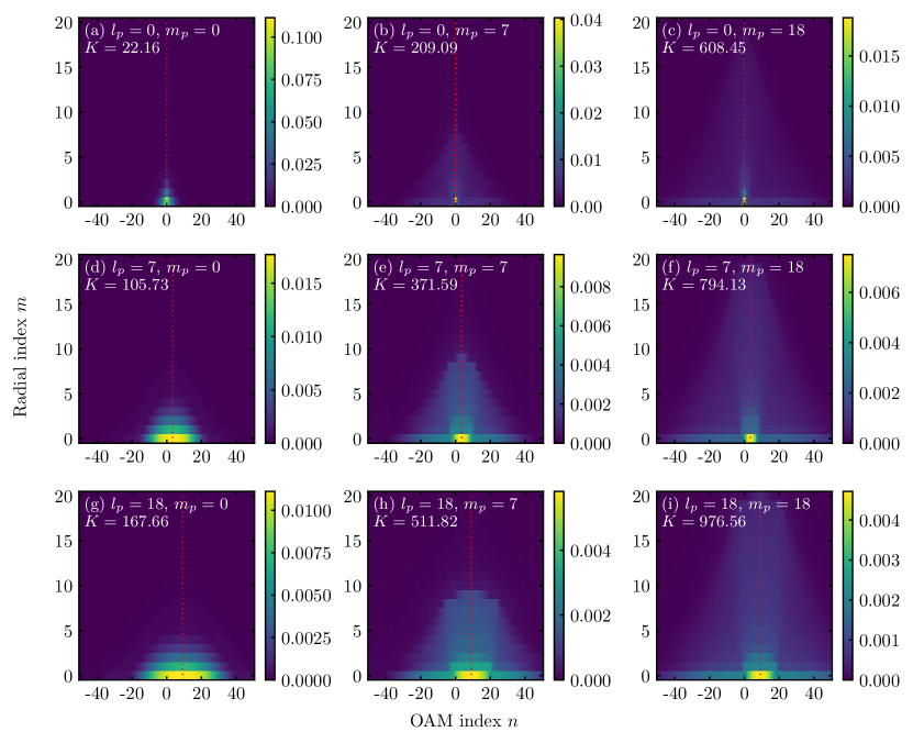
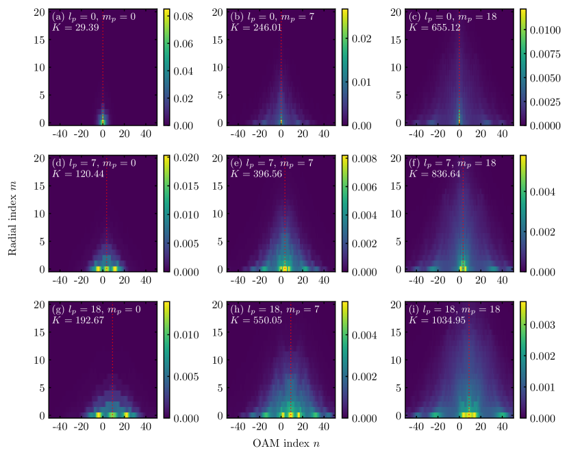
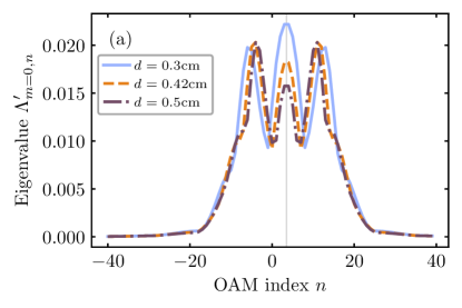
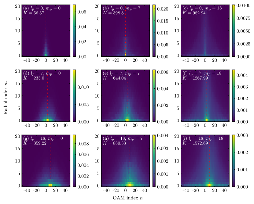
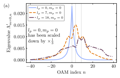
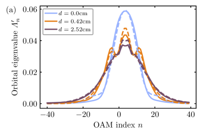
These eigenvalues determine the gain-dependent weights $\Lambda_{mn}^{\prime}$ [see Eqs. 2.39 and 2.40] of the corresponding Schmidt modes and are presented in Fig. 1 for different orbital $l_{p}$ and radial $m_{p}$ numbers of the pump. It can be seen that the widths of the distribution in the orbital $n$ and radial $m$ direction become larger with increasing orbital $l_{p}$ and radial $m_{p}$ numbers of the pump, respectively [see also Fig. 2(a)]. Therefore, by varying the parameters $l_{p}$ and $m_{p}$ of the pump beam, one can significantly increase the number of populated OAM and radial modes. To further quantify this, we also provide the Schmidt number (effective mode number) [11, 32]

$\displaystyle K$ $\displaystyle=\left[\sum_{m,n}\left(\Lambda_{mn}^{\prime}\right)^{2}\right]^{-1}$ (3.4)

in each 2D plot of eigenvalue distributions. As expected, the Schmidt number increases strongly as $l_{p}$ and $m_{p}$ are increased [see Fig. 1].

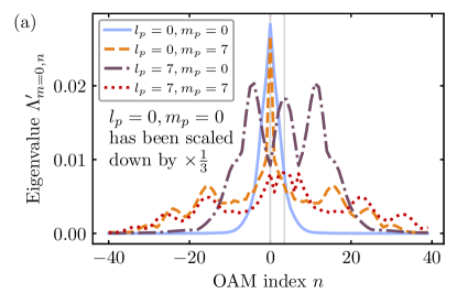
Furthermore, it is important to point out that the eigenvalue distribution is symmetric with respect to the axis $n=l_{p}/2$, see Figs. 1, 2(a) and 2(b). This means that for odd values of $l_{p}$, the distribution must be flat around the point $l_{p}/2$, since the eigenvalues to the left ($n=\lfloor l_{p}/2\rfloor$) and to the right ($n=\lceil l_{p}/2\rceil$) of this point must be identical, see Fig. 2(a).

Refer to caption
((a))
Refer to caption
((b))
Refer to caption
((c))
Refer to caption
((d))
Figure 2: Cuts of the normalized modal weights Λm=0,nsubscriptsuperscriptΛ𝑚0𝑛\Lambda^{\prime}_{m=0,n} (m,nΛmn=1subscript𝑚𝑛subscriptsuperscriptΛ𝑚𝑛1{\sum_{m,n}\Lambda^{\prime}_{mn}}=1) for the (a) low-gain and (b) high-gain regime for a single BBO crystal of length L=2 mm𝐿times2millimeterL=$2\text{\,}\mathrm{mm}$. The thin gray lines indicate n=0𝑛0n=0 and n=3.5𝑛3.5n=3.5, which are the symmetry lines for lp=0subscript𝑙𝑝0l_{p}=0 and lp=7subscript𝑙𝑝7l_{p}=7, respectively. The plots (a) and (b) clearly show an increase in the width in the orbital direction (along n𝑛n) when increasing the radial mpsubscript𝑚𝑝m_{p} and orbital lpsubscript𝑙𝑝l_{p} numbers of the pump. Normalized intensity spectra for the (c) low-gain and (d) high-gain regime. For lp=0subscript𝑙𝑝0l_{p}=0 and mp=0subscript𝑚𝑝0m_{p}=0 the intensity distribution has a sinc2superscriptsinc2\operatorname{sinc}^{2}-shape. The intensity profile becomes more Gaussian as lpsubscript𝑙𝑝l_{p} and mpsubscript𝑚𝑝m_{p} increases.

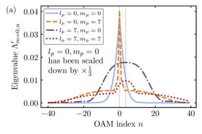
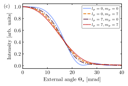
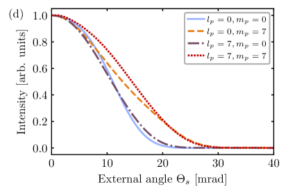
For the low-gain regime, the shapes of the intensity spectra for different orbital and radial numbers are shown in Fig. 2(c). They are formed by several Schmidt modes with the weights $\lambda_{mn}$ according to Eqs. 2.38 and 2.40. For $l_{p}=0$ and $m_{p}=0$ the intensity distribution has a $\operatorname{sinc}^{2}$-shape. The intensity profile becomes more Gaussian with increasing $m_{p}$, since the contribution of the fundamental mode (which is Gaussian) becomes higher compared to other modes, see orange curve in Fig. 2(a), see also Ref. 11. For nonzero $l_{p}$, even though the mode with the largest population is not Gaussian, the number of modes contributing to the total intensity is large enough, so the intensity profile still has a shape which is close to Gaussian.

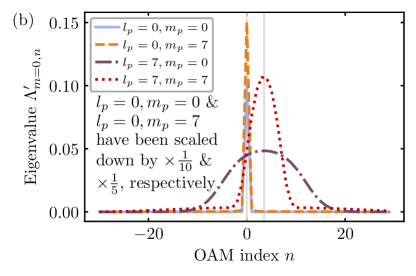
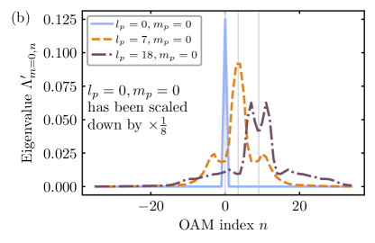
As we move to the high-gain regime, shown in Fig. 2(b), the eigenvalues are redistributed compared to the low-gain regime [11] [see Fig. 2(a)] according to Eq. 2.40 and fewer Schmidt modes contribute to the shape of the intensity spectrum. By reducing the number of contributing modes the eigenvalue distributions and intensity profiles get narrower. Moreover, it can be seen that as $l_{p}$ and $m_{p}$ increase, the intensity distribution becomes wider due to larger mode widths for higher $l_{p}$ and $m_{p}$.

III.2 Two-crystal setup

An SU(1,1) interferometer consists of two PDC sections with a linear medium in-between. This linear medium imprints a (possibly spatially varying) phase to the pump, signal and idler radiation [22, 23, 32, 21]. In this section, we consider a phase which is simply given by the air gap of length $d$ between the two crystals. The function $g_{z}$ for the two-crystal setup can then be written in the form [11]:

$\displaystyle\begin{split}g_{z}\mathchoice{\!\left({q_{s},q_{i},\phi_{s},\phi_{i}}\right)}{\!\left({q_{s},q_{i},\phi_{s},\phi_{i}}\right)}{\left({q_{s},q_{i},\phi_{s},\phi_{i}}\right)}{\left({q_{s},q_{i},\phi_{s},\phi_{i}}\right)}&=2L\operatorname{sinc}\mathchoice{\!\left({L\frac{(\boldsymbol{q}_{s}-\boldsymbol{q}_{i})^{2}}{4k_{p}}}\right)}{\!\left({L\frac{(\boldsymbol{q}_{s}-\boldsymbol{q}_{i})^{2}}{4k_{p}}}\right)}{\left({L\frac{(\boldsymbol{q}_{s}-\boldsymbol{q}_{i})^{2}}{4k_{p}}}\right)}{\left({L\frac{(\boldsymbol{q}_{s}-\boldsymbol{q}_{i})^{2}}{4k_{p}}}\right)}\cos\mathchoice{\!\left[{L\frac{(\boldsymbol{q}_{s}-\boldsymbol{q}_{i})^{2}}{4k_{p}}+\frac{\Delta nk_{s}d}{n_{s}}+n_{s}d\frac{(\boldsymbol{q}_{s}-\boldsymbol{q}_{i})^{2}}{4k_{p}}}\right]}{\!\left[{L\frac{(\boldsymbol{q}_{s}-\boldsymbol{q}_{i})^{2}}{4k_{p}}+\frac{\Delta nk_{s}d}{n_{s}}+n_{s}d\frac{(\boldsymbol{q}_{s}-\boldsymbol{q}_{i})^{2}}{4k_{p}}}\right]}{\left[{L\frac{(\boldsymbol{q}_{s}-\boldsymbol{q}_{i})^{2}}{4k_{p}}+\frac{\Delta nk_{s}d}{n_{s}}+n_{s}d\frac{(\boldsymbol{q}_{s}-\boldsymbol{q}_{i})^{2}}{4k_{p}}}\right]}{\left[{L\frac{(\boldsymbol{q}_{s}-\boldsymbol{q}_{i})^{2}}{4k_{p}}+\frac{\Delta nk_{s}d}{n_{s}}+n_{s}d\frac{(\boldsymbol{q}_{s}-\boldsymbol{q}_{i})^{2}}{4k_{p}}}\right]}\\ &\qquad\times\exp\mathchoice{\!\left[{\mathrm{i}\left(L\frac{(\boldsymbol{q_{s}}-\boldsymbol{q}_{i})^{2}}{2k_{p}}+\frac{\Delta nk_{s}d}{n_{s}}+n_{s}d\frac{(\boldsymbol{q}_{s}-\boldsymbol{q}_{i})^{2}}{4k_{p}}\right)}\right]}{\!\left[{\mathrm{i}\left(L\frac{(\boldsymbol{q_{s}}-\boldsymbol{q}_{i})^{2}}{2k_{p}}+\frac{\Delta nk_{s}d}{n_{s}}+n_{s}d\frac{(\boldsymbol{q}_{s}-\boldsymbol{q}_{i})^{2}}{4k_{p}}\right)}\right]}{\left[{\mathrm{i}\left(L\frac{(\boldsymbol{q_{s}}-\boldsymbol{q}_{i})^{2}}{2k_{p}}+\frac{\Delta nk_{s}d}{n_{s}}+n_{s}d\frac{(\boldsymbol{q}_{s}-\boldsymbol{q}_{i})^{2}}{4k_{p}}\right)}\right]}{\left[{\mathrm{i}\left(L\frac{(\boldsymbol{q_{s}}-\boldsymbol{q}_{i})^{2}}{2k_{p}}+\frac{\Delta nk_{s}d}{n_{s}}+n_{s}d\frac{(\boldsymbol{q}_{s}-\boldsymbol{q}_{i})^{2}}{4k_{p}}\right)}\right]},\end{split}$ (3.5)

where $\Delta n=n^{\mathrm{air}}_{p}-\frac{1}{2}(n^{\mathrm{air}}_{s}+n^{\mathrm{air}}_{i})=n^{\mathrm{air}}_{p}-n^{\mathrm{air}}_{s}$ and $n^{\mathrm{air}}_{j}$ ($j=p,s,i$) are the refractive indices of the pump, signal and idler radiation in the air gap between the two crystals, while $n_{s}$ is the refractive index of the signal beam inside the crystal. Here, the Fresnel approximation has again been applied and perfect phase matching is assumed for the collinear direction (where $\boldsymbol{q}_{s}=\boldsymbol{q}_{i}=\boldsymbol{0}$), just as in Sec. III.1 for the single crystal.

Refer to caption
Figure 3: Integral intensity of the SU(1,1) interferometer output over the distance between the two crystals. The thin gray lines indicate the distances for which the first minimum at d=0.42 cm𝑑times0.42centimeterd=$0.42\text{\,}\mathrm{cm}$ and the first maximum at d=2.52 cm𝑑times2.52centimeterd=$2.52\text{\,}\mathrm{cm}$ are observed. Note that the position of the bright and dark fringe seem to be independent of lpsubscript𝑙𝑝l_{p} and mpsubscript𝑚𝑝m_{p}. To verify this, we compared all 64 combinations of lpsubscript𝑙𝑝l_{p} and mpsubscript𝑚𝑝m_{p} from 0 to 7 and found that for different lpsubscript𝑙𝑝l_{p} and mpsubscript𝑚𝑝m_{p} the integral intensities show no significant differences compared to each other and only differ by a scaling factor.

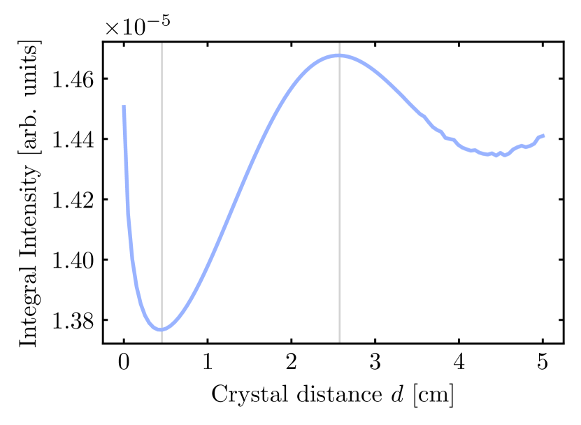
Figure 3 presents the integral intensity over the distance d𝑑d between the crystals that is obtained by integrating the intensity distribution Eq. 2.38 over the radial and azimuthal variables. Here, starting near d=3.2 cm𝑑times3.2centimeterd=$3.2\text{\,}\mathrm{cm}$, numerical noise becomes visible. This is caused by the interference in the second crystal which results in peaks in the intensity spectrum that become denser as d𝑑d increases and are at some point no longer resolved with the chosen numerical grid. Below we will only pay attention to the two special points of this dependence, namely, the first minimum (d=0.42 cm𝑑times0.42centimeterd=$0.42\text{\,}\mathrm{cm}$, dark fringe) and the first maximum (d=2.52 cm𝑑times2.52centimeterd=$2.52\text{\,}\mathrm{cm}$, bright fringe), which are shown by the thin gray lines in Fig. 3.

III.2.1 Dark fringe

Figure 4 shows the normalized eigenvalue distribution for the first minimum of the total intensity distribution (d=0.42 cm𝑑times0.42centimeterd=$0.42\text{\,}\mathrm{cm}$) for different orbital lpsubscript𝑙𝑝l_{p} and radial mpsubscript𝑚𝑝m_{p} numbers of the pump. It can be seen that the eigenvalue distribution becomes broader and the Schmidt number K𝐾K is increased for an SU(1,1) interferometer setup compared to the single-crystal setup for the same values of lpsubscript𝑙𝑝l_{p} and mpsubscript𝑚𝑝m_{p} (compare Figs. 1 and 4).

Furthermore, one can observe that, contrary to the single-crystal configuration, the normalized eigenvalue distributions in the dark-fringe case are characterized by non-monotonic behavior along the orbital direction $n$.

Refer to caption
Figure 4: Normalized modal weight spectra ΛmnsubscriptsuperscriptΛ𝑚𝑛\Lambda^{\prime}_{mn} (m,nΛmn=1subscript𝑚𝑛subscriptsuperscriptΛ𝑚𝑛1{\sum_{m,n}\Lambda^{\prime}_{mn}}=1) for the low-gain regime (G=0.01𝐺0.01G=0.01), for the two-crystal setup (two BBO crystals, each of length L=2 mm𝐿times2millimeterL=$2\text{\,}\mathrm{mm}$) with an air gap of length d=0.42 cm𝑑times0.42centimeterd=$0.42\text{\,}\mathrm{cm}$ (dark fringe), pumped by a Laguerre-Gaussian pump with different combinations of orbital lpsubscript𝑙𝑝l_{p} and radial mpsubscript𝑚𝑝m_{p} indices as written in the plots. The red dotted lines indicate the symmetry axis of the eigenvalue distribution at n=lp/2𝑛subscript𝑙𝑝2n=l_{p}/2 (n=0𝑛0n=0, n=3.5𝑛3.5n=3.5 and n=9𝑛9n=9, for lp=0subscript𝑙𝑝0l_{p}=0, lp=7subscript𝑙𝑝7l_{p}=7 and lp=18subscript𝑙𝑝18l_{p}=18, respectively). The graphs clearly show non-monotonic behavior for the eigenvalue distributions along the orbital direction n𝑛n and an increase in the Schmidt number compared to the single-crystal case (presented in Fig. 1).

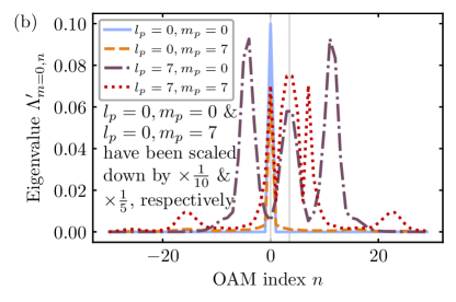
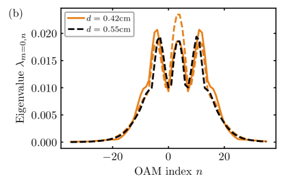
This non-monotonic behavior is observed for nonzero orbital/radial pump numbers and is more clearly visible in the $\lambda_{m=0,n}$ cuts of the modal weight distribution presented in Fig. 5(a). Furthermore, it can be seen that for nonzero orbital pump numbers, the orbital number of the PDC modes with the largest population is no longer $l_{p}/2$. For example, when $l_{p}=7$ and $m_{p}=0$, the mode with OAM $n=11$ has the highest population. In the high-gain regime, a repopulation of the modes takes place [11], and the modes with the largest weights are strongly amplified, see Fig. 5(b). This means that in the dark fringe, modes with an OAM higher than the pump OAM can be efficiently populated and filtered at high gain.

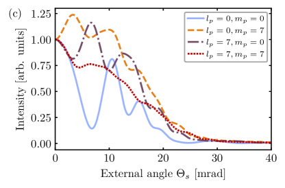
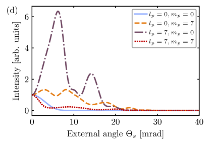
These non-trivial eigenvalue profiles result in the non-Gaussian intensity distributions with a complex shape presented in Figs. 5(c) and 5(d) for the low- and high-gain regimes, respectively. Some Schmidt modes which contribute to the intensity distribution are presented in Fig. 16 in Sec. A.1. A high population of modes with high-order OAM in the case of $l_{p}=7,m_{p}=0$ leads to a donut-shaped intensity profile with a local minimum in the center, which is most pronounced in the high-gain regime.

As already mentioned above, the eigenvalues are symmetrically populated around the point $l_{p}/2$, due to the fact that $\lambda_{m,l_{p}-n}=\lambda_{mn}$, see Eq. 2.29a. This means that if modes other than $l_{p}/2$ are most populated, then there is no single mode that uniquely determines the shape of the intensity distribution in the high-gain regime: There are at least two equally populated modes.

Refer to caption
((a))
Refer to caption
((b))
Refer to caption
((c))
Refer to caption
((d))
Figure 5: Cuts of the normalized modal weights Λm=0,nsubscriptsuperscriptΛ𝑚0𝑛\Lambda^{\prime}_{m=0,n} (m,nΛmn=1subscript𝑚𝑛subscriptsuperscriptΛ𝑚𝑛1{\sum_{m,n}\Lambda^{\prime}_{mn}}=1) for the (a) low-gain and (b) high-gain regime for two BBO crystals of length L=2 mm𝐿times2millimeterL=$2\text{\,}\mathrm{mm}$, an air gap between the crystals of length d=0.42 cm𝑑times0.42centimeterd=$0.42\text{\,}\mathrm{cm}$ (dark fringe) and different orbital lpsubscript𝑙𝑝l_{p} and radial mpsubscript𝑚𝑝m_{p} numbers of the pump as written in the plots. The thin gray lines indicate n=0𝑛0n=0 and n=3.5𝑛3.5n=3.5, which are the symmetry lines for lp=0subscript𝑙𝑝0l_{p}=0 and lp=7subscript𝑙𝑝7l_{p}=7, respectively. For a non-Gaussian pump, a non-monotonic behavior in the eigenvalue distribution can be observed. Normalized intensity spectra for the (c) low-gain and (d) high-gain regime. Due to the non-trivial behavior of the eigenvalue distribution, the intensities have a complex non-Gaussian shape at low and high gain.
Refer to caption
((a))
Refer to caption
((b))
Figure 6: Cuts of the normalized modal weights Λm=0,nsubscriptsuperscriptΛ𝑚0𝑛\Lambda^{\prime}_{m=0,n} (m,nΛmn=1subscript𝑚𝑛subscriptsuperscriptΛ𝑚𝑛1{\sum_{m,n}\Lambda^{\prime}_{mn}}=1) for lp=7subscript𝑙𝑝7l_{p}=7, mp=0subscript𝑚𝑝0m_{p}=0 for the (a) low-gain and (b) high-gain regime for different distances between the two crystals of an SU(1,1) interferometer around the dark fringe (d=0.42 cm𝑑times0.42centimeterd=$0.42\text{\,}\mathrm{cm}$). The thin gray lines indicate n=lp/2=3.5𝑛subscript𝑙𝑝23.5n=l_{p}/2=3.5. For the distances d=0.42 cm𝑑times0.42centimeterd=$0.42\text{\,}\mathrm{cm}$ and d=0.5 cm𝑑times0.5centimeterd=$0.5\text{\,}\mathrm{cm}$, the most populated OAM mode appears at n=11𝑛11n=11, which is higher than the pump OAM lp=7subscript𝑙𝑝7l_{p}=7. According to Eq. 2.40, the most populated OAM modes are strongly amplified in the high-gain regime [11]. See also Fig. 17 in Sec. A.2 which briefly discusses the case lp=18subscript𝑙𝑝18l_{p}=18.

By changing the distance between the crystals one can strongly modify the eigenvalue distribution and the OAM of the most populated mode. For example, varying the distance around the dark fringe point, one can change the OAM of the most populated mode from n=4𝑛4n=4 for d=0.3 cm𝑑times0.3centimeterd=$0.3\text{\,}\mathrm{cm}$ to n=11𝑛11n=11 for d=0.42 cm𝑑times0.42centimeterd=$0.42\text{\,}\mathrm{cm}$ and d=0.5 cm𝑑times0.5centimeterd=$0.5\text{\,}\mathrm{cm}$, see Fig. 6. See also Fig. 17 in Sec. A.2 where the case lp=18subscript𝑙𝑝18l_{p}=18 is discussed.

III.2.2 Bright fringe
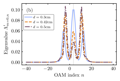
In the case of the bright fringe (d=2.52 cm𝑑times2.52centimeterd=$2.52\text{\,}\mathrm{cm}$), the non-monotonic behavior is less pronounced compared to the dark fringe, see Fig. 7, which shows the normalized eigenvalue distributions for the bright fringe for different orbital lpsubscript𝑙𝑝l_{p} and radial mpsubscript𝑚𝑝m_{p} numbers of the pump.

Refer to caption
Figure 7: Normalized modal weight spectra ΛmnsubscriptsuperscriptΛ𝑚𝑛\Lambda^{\prime}_{mn} (m,nΛmn=1subscript𝑚𝑛subscriptsuperscriptΛ𝑚𝑛1{\sum_{m,n}\Lambda^{\prime}_{mn}}=1) for the low-gain regime (G=0.01𝐺0.01G=0.01), for the two-crystal setup (two BBO crystals, each of length L=2 mm𝐿times2millimeterL=$2\text{\,}\mathrm{mm}$) with an air gap of length d=2.52 cm𝑑times2.52centimeterd=$2.52\text{\,}\mathrm{cm}$ (bright fringe), pumped by a Laguerre-Gaussian pump with different combinations of orbital lpsubscript𝑙𝑝l_{p} and radial mpsubscript𝑚𝑝m_{p} indices as written in the plots. The red dotted line indicates the symmetry axis of the eigenvalue distribution at n=lp/2𝑛subscript𝑙𝑝2n=l_{p}/2 (n=0𝑛0n=0, n=3.5𝑛3.5n=3.5 and n=9𝑛9n=9, for lp=0subscript𝑙𝑝0l_{p}=0, lp=7subscript𝑙𝑝7l_{p}=7 and lp=18subscript𝑙𝑝18l_{p}=18, respectively).

However, the cuts of the modal weights $\Lambda_{m=0,n}$ presented in Fig. 8 clearly demonstrate that this behavior also occurs here, while changing in the pump OAM modifies the OAM of the most populated mode [see Fig. 8(a)]. Similarly to the dark fringe, the high-gain regime allows us to filter these most populated modes, see Fig. 8(b).

Refer to caption
((a))
Refer to caption
((b))
Figure 8: Cuts of the normalized modal weights Λm=0,nsubscriptsuperscriptΛ𝑚0𝑛\Lambda^{\prime}_{m=0,n} (m,nΛmn=1subscript𝑚𝑛subscriptsuperscriptΛ𝑚𝑛1{\sum_{m,n}\Lambda^{\prime}_{mn}}=1) for the (a) low-gain and (b) high-gain regime for two BBO crystals of length L=2 mm𝐿times2millimeterL=$2\text{\,}\mathrm{mm}$, an air gap of length d=2.52 cm𝑑times2.52centimeterd=$2.52\text{\,}\mathrm{cm}$ (bright fringe) between the crystals and different orbital lpsubscript𝑙𝑝l_{p} and radial mpsubscript𝑚𝑝m_{p} numbers of the pump as written in the plots. The thin gray lines indicate n=0𝑛0n=0, n=3.5𝑛3.5n=3.5 and n=9𝑛9n=9, which are the symmetry lines for lp=0subscript𝑙𝑝0l_{p}=0, lp=7subscript𝑙𝑝7l_{p}=7 and lp=18subscript𝑙𝑝18l_{p}=18, respectively. Increasing the pump OAM lpsubscript𝑙𝑝l_{p} changes the order of the most populated OAM modes.

III.3 Non-monotonic behavior

As was demonstrated in the previous section, configurations of two crystals with a nonzero distance between the crystals and non-Gaussian pumping can result in a non-monotonic structure of the eigenvalue distribution. This non-monotonic behavior is not observed for a single crystal pumped by a non-Gaussian pump and leads to configurations where the highest population of modes occurs at an OAM higher than the pump OAM.

To investigate the non-monotonic behavior in more detail, we focus on the orbital eigenvalues in the low-gain regime

$\displaystyle\varLambda_{n}\overset{\mathrm{def.}}{=}\sum_{m}\lambda_{mn},$ (3.6)

which are the probabilities to find a Schmidt mode with OAM $n$ in the signal/idler field. The orbital eigenvalues can also be obtained by integrating the Fourier coefficients $\chi_{n}\mathchoice{\!\left({q_{s},q_{i}}\right)}{\!\left({q_{s},q_{i}}\right)}{\left({q_{s},q_{i}}\right)}{\left({q_{s},q_{i}}\right)}$ introduced in Eq. 2.19, namely,

$\displaystyle\varLambda_{n}=\iint\!\mathrm{d}q_{s}\mathrm{d}q_{i}\,q_{s}q_{i}{\mathchoice{{\kern 0.41667pt}}{}{}{}|}\chi_{n}\mathchoice{\!\left({q_{s},q_{i}}\right)}{\!\left({q_{s},q_{i}}\right)}{\left({q_{s},q_{i}}\right)}{\left({q_{s},q_{i}}\right)}{|\mathchoice{{\kern 0.41667pt}}{}{}{}}^{2}.$ (3.7)

Since the non-monotonic behavior has been observed for any nonzero $l_{p}$ and any $m_{p}$, we set $m_{p}=0$ for simplicity, so that the Laguerre polynomials in the pump envelope [Eq. 2.3] are equal to $1$, regardless of the value of $l_{p}$. We also define the (complex) constant

$\displaystyle\bar{A}\overset{\mathrm{def.}}{=}4CL\pi^{2}\left(-1\right)^{l_{p}}\mathrm{i}^{|l_{p}|}\left(\frac{w_{0}}{2}\right)^{|l_{p}|+1},$ (3.8)

which includes all prefactors of $R$ that do not depend on $q_{s}$, $q_{i}$, $\phi_{s}$ or $\phi_{i}$ [compare Eq. 2.15].

In order to allow for an analytical treatment, we use the Gaussian approximation $\operatorname{sinc}\mathchoice{\!\left({b^{2}x^{2}}\right)}{\!\left({b^{2}x^{2}}\right)}{\left({b^{2}x^{2}}\right)}{\left({b^{2}x^{2}}\right)}\approx\exp\mathchoice{\!\left({-\alpha^{2}b^{2}x^{2}}\right)}{\!\left({-\alpha^{2}b^{2}x^{2}}\right)}{\left({-\alpha^{2}b^{2}x^{2}}\right)}{\left({-\alpha^{2}b^{2}x^{2}}\right)}$ for the $\operatorname{sinc}$-function appearing in $g_{z}$ in Eq. 3.5, where ${\alpha=0.65}$ is an additional heuristic scaling factor to achieve a good approximation [10].

The function $g_{z}$ is then given by

$\displaystyle\begin{split}g_{z}\mathchoice{\!\left({q_{s},q_{i},\phi_{s},\phi_{i}}\right)}{\!\left({q_{s},q_{i},\phi_{s},\phi_{i}}\right)}{\left({q_{s},q_{i},\phi_{s},\phi_{i}}\right)}{\left({q_{s},q_{i},\phi_{s},\phi_{i}}\right)}&=2L\exp\mathchoice{\!\left({-\alpha^{2}L\frac{(\boldsymbol{q}_{s}-\boldsymbol{q}_{i})^{2}}{4k_{p}}}\right)}{\!\left({-\alpha^{2}L\frac{(\boldsymbol{q}_{s}-\boldsymbol{q}_{i})^{2}}{4k_{p}}}\right)}{\left({-\alpha^{2}L\frac{(\boldsymbol{q}_{s}-\boldsymbol{q}_{i})^{2}}{4k_{p}}}\right)}{\left({-\alpha^{2}L\frac{(\boldsymbol{q}_{s}-\boldsymbol{q}_{i})^{2}}{4k_{p}}}\right)}\cos\mathchoice{\!\left({L\frac{(\boldsymbol{q}_{s}-\boldsymbol{q}_{i})^{2}}{4k_{p}}+\frac{\Delta nk_{s}d}{n_{s}}+n_{s}d\frac{(\boldsymbol{q}_{s}-\boldsymbol{q}_{i})^{2}}{4k_{p}}}\right)}{\!\left({L\frac{(\boldsymbol{q}_{s}-\boldsymbol{q}_{i})^{2}}{4k_{p}}+\frac{\Delta nk_{s}d}{n_{s}}+n_{s}d\frac{(\boldsymbol{q}_{s}-\boldsymbol{q}_{i})^{2}}{4k_{p}}}\right)}{\left({L\frac{(\boldsymbol{q}_{s}-\boldsymbol{q}_{i})^{2}}{4k_{p}}+\frac{\Delta nk_{s}d}{n_{s}}+n_{s}d\frac{(\boldsymbol{q}_{s}-\boldsymbol{q}_{i})^{2}}{4k_{p}}}\right)}{\left({L\frac{(\boldsymbol{q}_{s}-\boldsymbol{q}_{i})^{2}}{4k_{p}}+\frac{\Delta nk_{s}d}{n_{s}}+n_{s}d\frac{(\boldsymbol{q}_{s}-\boldsymbol{q}_{i})^{2}}{4k_{p}}}\right)}\\ &\qquad\times\exp\mathchoice{\!\left[{\mathrm{i}\left(L\frac{(\boldsymbol{q_{s}}-\boldsymbol{q}_{i})^{2}}{2k_{p}}+\frac{\Delta nk_{s}d}{n_{s}}+n_{s}d\frac{(\boldsymbol{q}_{s}-\boldsymbol{q}_{i})^{2}}{4k_{p}}\right)}\right]}{\!\left[{\mathrm{i}\left(L\frac{(\boldsymbol{q_{s}}-\boldsymbol{q}_{i})^{2}}{2k_{p}}+\frac{\Delta nk_{s}d}{n_{s}}+n_{s}d\frac{(\boldsymbol{q}_{s}-\boldsymbol{q}_{i})^{2}}{4k_{p}}\right)}\right]}{\left[{\mathrm{i}\left(L\frac{(\boldsymbol{q_{s}}-\boldsymbol{q}_{i})^{2}}{2k_{p}}+\frac{\Delta nk_{s}d}{n_{s}}+n_{s}d\frac{(\boldsymbol{q}_{s}-\boldsymbol{q}_{i})^{2}}{4k_{p}}\right)}\right]}{\left[{\mathrm{i}\left(L\frac{(\boldsymbol{q_{s}}-\boldsymbol{q}_{i})^{2}}{2k_{p}}+\frac{\Delta nk_{s}d}{n_{s}}+n_{s}d\frac{(\boldsymbol{q}_{s}-\boldsymbol{q}_{i})^{2}}{4k_{p}}\right)}\right]}.\end{split}$ (3.9)

Next, we expand $W\mathchoice{\!\left({q_{s},q_{i},\phi_{s}-\phi_{i}}\right)}{\!\left({q_{s},q_{i},\phi_{s}-\phi_{i}}\right)}{\left({q_{s},q_{i},\phi_{s}-\phi_{i}}\right)}{\left({q_{s},q_{i},\phi_{s}-\phi_{i}}\right)}$ defined in Eq. 2.13b using the binomial theorem and abbreviate the angle difference as $\phi_{s}-\phi_{i}\overset{\mathrm{def.}}{=}\phi$. The Fourier integral from Eq. 2.17 is then given by:

$\displaystyle\begin{split}\chi_{n}\mathchoice{\!\left({q_{s},q_{i}}\right)}{\!\left({q_{s},q_{i}}\right)}{\left({q_{s},q_{i}}\right)}{\left({q_{s},q_{i}}\right)}&=\bar{A}\int_{0}^{2\pi}\!\mathrm{d}\phi\,\exp\mathchoice{\!\left[{-L\alpha^{2}\frac{(\boldsymbol{q}_{s}-\boldsymbol{q}_{i})^{2}}{4k_{p}}-\left(\frac{w_{0}\xi}{2}\right)^{2}+\mathrm{i}\left(L\frac{(\boldsymbol{q}_{s}-\boldsymbol{q}_{i})^{2}}{2k_{p}}+\frac{\Delta nk_{s}d}{n_{s}}+n_{s}d\frac{(\boldsymbol{q}_{s}-\boldsymbol{q}_{i})^{2}}{4k_{p}}\right)}\right]}{\!\left[{-L\alpha^{2}\frac{(\boldsymbol{q}_{s}-\boldsymbol{q}_{i})^{2}}{4k_{p}}-\left(\frac{w_{0}\xi}{2}\right)^{2}+\mathrm{i}\left(L\frac{(\boldsymbol{q}_{s}-\boldsymbol{q}_{i})^{2}}{2k_{p}}+\frac{\Delta nk_{s}d}{n_{s}}+n_{s}d\frac{(\boldsymbol{q}_{s}-\boldsymbol{q}_{i})^{2}}{4k_{p}}\right)}\right]}{\left[{-L\alpha^{2}\frac{(\boldsymbol{q}_{s}-\boldsymbol{q}_{i})^{2}}{4k_{p}}-\left(\frac{w_{0}\xi}{2}\right)^{2}+\mathrm{i}\left(L\frac{(\boldsymbol{q}_{s}-\boldsymbol{q}_{i})^{2}}{2k_{p}}+\frac{\Delta nk_{s}d}{n_{s}}+n_{s}d\frac{(\boldsymbol{q}_{s}-\boldsymbol{q}_{i})^{2}}{4k_{p}}\right)}\right]}{\left[{-L\alpha^{2}\frac{(\boldsymbol{q}_{s}-\boldsymbol{q}_{i})^{2}}{4k_{p}}-\left(\frac{w_{0}\xi}{2}\right)^{2}+\mathrm{i}\left(L\frac{(\boldsymbol{q}_{s}-\boldsymbol{q}_{i})^{2}}{2k_{p}}+\frac{\Delta nk_{s}d}{n_{s}}+n_{s}d\frac{(\boldsymbol{q}_{s}-\boldsymbol{q}_{i})^{2}}{4k_{p}}\right)}\right]}\\ &\qquad\times\cos\mathchoice{\!\left({L\frac{\left(\boldsymbol{q}_{s}-\boldsymbol{q}_{i}\right)^{2}}{4k_{p}}+\frac{\Delta nk_{s}d}{n_{s}}+n_{s}d\frac{\left(\boldsymbol{q}_{s}-\boldsymbol{q}_{i}\right)^{2}}{4k_{p}}}\right)}{\!\left({L\frac{\left(\boldsymbol{q}_{s}-\boldsymbol{q}_{i}\right)^{2}}{4k_{p}}+\frac{\Delta nk_{s}d}{n_{s}}+n_{s}d\frac{\left(\boldsymbol{q}_{s}-\boldsymbol{q}_{i}\right)^{2}}{4k_{p}}}\right)}{\left({L\frac{\left(\boldsymbol{q}_{s}-\boldsymbol{q}_{i}\right)^{2}}{4k_{p}}+\frac{\Delta nk_{s}d}{n_{s}}+n_{s}d\frac{\left(\boldsymbol{q}_{s}-\boldsymbol{q}_{i}\right)^{2}}{4k_{p}}}\right)}{\left({L\frac{\left(\boldsymbol{q}_{s}-\boldsymbol{q}_{i}\right)^{2}}{4k_{p}}+\frac{\Delta nk_{s}d}{n_{s}}+n_{s}d\frac{\left(\boldsymbol{q}_{s}-\boldsymbol{q}_{i}\right)^{2}}{4k_{p}}}\right)}\sum_{\nu=0}^{l_{p}}\binom{l_{p}}{\nu}q_{s}^{\nu}q^{l_{p}-\nu}_{i}\mathrm{e}^{\mathrm{i}\left(n-\nu\right)\phi}.\end{split}$ (3.10)

By analytically evaluating the integral over $\phi$ in the expression above and integrating ${\mathchoice{{\kern 0.41667pt}}{}{}{}|}\chi_{n}\mathchoice{\!\left({q_{s},q_{i}}\right)}{\!\left({q_{s},q_{i}}\right)}{\left({q_{s},q_{i}}\right)}{\left({q_{s},q_{i}}\right)}{|\mathchoice{{\kern 0.41667pt}}{}{}{}}^{2}$ over $q_{s}$ and $q_{i}$, one can obtain the orbital eigenvalues $\varLambda_{n}$ according to Eq. 3.7:

$\displaystyle\begin{split}\varLambda_{n}&=A^{\prime}\int_{0}^{\infty}\!\int_{0}^{\infty}\!\mathrm{d}q_{s}\mathrm{d}q_{i}\,q_{s}q_{i}\mathrm{e}^{-a\left(q_{s}^{2}+q_{i}^{2}\right)}\left|\sum_{\nu=0}^{l_{p}}\binom{l_{p}}{\nu}q_{s}^{\nu}q^{l_{p}-\nu}_{i}\left[\mathrm{e}^{\mathrm{i}\frac{E}{2}(q_{s}^{2}+q_{i}^{2})}\mathrm{e}^{\mathrm{i}\mu}J_{n-\nu}\mathchoice{\!\left({q_{s}q_{i}V}\right)}{\!\left({q_{s}q_{i}V}\right)}{\left({q_{s}q_{i}V}\right)}{\left({q_{s}q_{i}V}\right)}+\mathrm{e}^{-\mathrm{i}\frac{E}{2}(q_{s}^{2}+q_{i}^{2})}\mathrm{e}^{-\mathrm{i}\mu}J_{n-\nu}\mathchoice{\!\left({q_{s}q_{i}U}\right)}{\!\left({q_{s}q_{i}U}\right)}{\left({q_{s}q_{i}U}\right)}{\left({q_{s}q_{i}U}\right)}\right]\right|^{2},\end{split}$ (3.11a)
where $J_{n-\nu}$ denotes the Bessel functions of order $n-\nu$ and
$\displaystyle A^{\prime}$ $\displaystyle=\bar{A}\pi,$ (3.11b)
$\displaystyle a$ $\displaystyle=\frac{w_{0}^{2}}{2}+\frac{L\alpha^{2}}{2k_{p}},$ (3.11c)
$\displaystyle E$ $\displaystyle=\frac{L}{2k_{p}}+\frac{n_{s}d}{2k_{p}},$ (3.11d)
$\displaystyle\mu$ $\displaystyle=\frac{\Delta nk_{s}d}{n_{s}},$ (3.11e)
$\displaystyle V$ $\displaystyle=\frac{\mathrm{i}w_{0}^{2}}{2}-\frac{\mathrm{i}L\alpha^{2}}{2k_{p}}-\frac{3L}{2k_{p}}-\frac{n_{s}d}{k_{p}},$ (3.11f)
$\displaystyle U$ $\displaystyle=\frac{\mathrm{i}w_{0}^{2}}{2}-\frac{\mathrm{i}L\alpha^{2}}{2k_{p}}-\frac{L}{2k_{p}}.$ (3.11g)

From Eq. 3.11a it can be seen that for $d=0$, the profile of orbital eigenvalue distribution is defined by a Binomial distribution and the most populated mode has the OAM $n=l_{p}/2$, while the distribution has a monotonic behavior. However, for $d>0$, a complicated interference takes place (see the term in the brackets) due to the nonzero $\mu=\Delta nk_{s}d/n_{s}$ factor. This leads to the suppression of low-order Bessel terms and enhanced contribution of high-order Bessel functions to the eigenvalue distribution, resulting in the non-monotonic behavior. To demonstrate this, we plot the $\varLambda_{n}$ obtained from the analytical expression [Eq. 3.11a] with the Double-Gaussian approximation for different distances between the crystals, see Fig. 9(a) (dashed lines).

It can be seen that a non-monotonic behavior takes place for both constructive and destructive interference points, however, it is more pronounced for the destructive interference configuration. For $d=0$ the distribution is centred at $n=l_{p}/2$ and, as predicted, has a monotonic behavior. In the same plot, the numerically calculated orbital eigenvalues [obtained using $g_{z}$ with the $\operatorname{sinc}$-term as in Eq. 3.5] are presented by solid lines. The good agreement between the numerically calculated and analytically evaluated orbital eigenvalues demonstrates the validity of the approximated analytical expression Eq. 3.11a.

The modal weight cuts also demonstrate a qualitative similarity between the two models, see Fig. 9(b), where they are presented for the dark fringe of the interferometer. It is worth noting that in the Double-Gaussian approximation, the point of the dark fringe is shifted, and therefore, the side peaks for the crystal distance d=0.42 cm𝑑times0.42centimeterd=$0.42\text{\,}\mathrm{cm}$ are not as pronounced as in the case including the sincsinc\operatorname{sinc}-term. However, for the distance d=0.55 cm𝑑times0.55centimeter{d=$0.55\text{\,}\mathrm{cm}$}, we obtain the same picture with more pronounced side peaks compared to the symmetry point lp/2subscript𝑙𝑝2l_{p}/2 in the Double-Gaussian approximation.

Refer to caption
((a))
Refer to caption
((b))
Figure 9: (a) Normalized orbital eigenvalues $\varLambda_{n}^{\prime}=\varLambda_{n}/\sum_{n}\varLambda_{n}$ and (b) cuts of the normalized low-gain modal weights $\lambda_{m=0,n}$ (${\sum_{m,n}\lambda_{mn}}=1$) for different distances $d$ between the two crystals of the SU(1,1) interferometer. Pump parameters are $l_{p}=7$ and $m_{p}=0$. The curves are calculated using $g_{z}$ in the form of the $\operatorname{sinc}$-term as in Eq. 3.5 (solid lines) and using the double Gaussian approximation [Eq. 3.11a, dashed lines].

IV ANGULAR DISPLACEMENT MEASUREMENT

In this section, we finalize our analysis of PDC with Laguerre-Gaussian pump beams by analyzing the application of the SU(1,1) interferometer for angular displacement detection. As it has already been mentioned in Sec. I, it is possible to use entangled photon states to reach supersensitivity for angular displacement detection [8, 17, 18]. In this section, to beat the classical limit, we consider an SU(1,1) interferometer which has a Dove prism placed between the two crystals. A sketch of this setup is presented in Fig. 10.

Refer to caption

Detection

$\theta$
Dove prism
Signal/idler
radiation
Crystal 1
Crystal 2
Lens 2
Lens 1
$E_{p}^{\left(1\right)}$
$E_{p}^{\left(2\right)}$
$l_{p}$
$-l_{p}$
Flat phase
Crystal 2
$E_{p}^{\left(2\right)}$
$l_{p}$

Detection

$\mathrm{e}^{-\mathrm{i}l_{p}\theta}$
Figure 10: Left: Sketch of the SU(1,1) interferometer in diffraction compensated configuration (4f-lens system[32] with a Dove prism rotated by an angle $\theta$ and located between the two lenses in the signal and idler field. The first crystal is pumped by a Laguerre-Gaussian beam $E_{p}^{\left(1\right)}$ with OAM $l_{p}$, while the second crystal is pumped by a Laugerre-Gaussian beam $E_{p}^{\left(2\right)}$ with OAM $-l_{p}$. In an experimental setup, the pump fields can usually be removed after the first crystal and before the detection stage using a dichroic mirror (not shown). Mathematically, the lenses are taken into account via Eq. 4.8 [32]. Right: Interpretation of the dashed rectangle on the left. As described in the text, the setup shown on the left is mathematically equivalent to instead pumping the second crystal with a Laguerre-Gaussian beam $E_{p}^{\left(2\right)}$ with OAM $l_{p}$ (same sign as for the first crystal) and adding a flat (constant with respect to $\boldsymbol{q}_{p}$, $\boldsymbol{q}_{s}$ and $\boldsymbol{q}_{i}$) phase profile $\mathrm{e}^{-\mathrm{i}l_{p}\theta}$ to the signal and idler radiation (or, equivalently, to the pump beam), which results in an additional phase factor in the second crystal’s TPA, see Eq. 4.7. The structure of the system is then equivalent to the compensated SU(1,1) interferometer considered in Ref. 32, except for the pump shape and the fact that therein, only one transverse dimension is considered. Note that in both the left and right part of the figure, the superscript (2,D) used in the text refers to the subsystem marked with the dashed rectangle.

A Dove prism modifies the electric signal and idler fields in two ways, provided that the fields are not too tightly focused [34, 18]: First, it swaps the helicity of the OAM components of the electric field. For example, if the signal field inside the interferometer (the radiation generated from the first crystal) has an azimuthal dependency $\mathrm{e}^{\mathrm{i}n\phi_{s}}$ for some $n\in\mathbb{Z}$, then after the prism it is given by $\mathrm{e}^{-\mathrm{i}n\phi_{s}}$ and, analogously, the helicity is swapped for the idler field. Second, the prism introduces a phase $\mathrm{e}^{-\mathrm{i}n{\theta}}$ to the field, where $\theta$ is the rotation angle of the prism. Note that in our system, this phase is added for both the signal and idler field.

To understand the impact these actions have on the SU(1,1) interferometer, we first analyze the symmetries of the system under a sign change of the pump OAM index. Intuitively, if the sign of $l_{p}$ is changed, $l_{p}\rightarrow-l_{p}$, the results presented in this work should not be affected qualitatively and only change by certain symmetry transformations. To analyze this more rigorously, we add a superscript ${}^{\left[l_{p}\right]}$ or ${}^{\left[-l_{p}\right]}$ to the quantities in question, depending on the sign of the pump OAM number.

With this notation, it is immediately clear that for the function $W$ as defined in Eq. 2.13b,

$\displaystyle W^{\left[l_{p}\right]}\mathchoice{\!\left({q_{s},q_{i},\phi_{s}-\phi_{i}}\right)}{\!\left({q_{s},q_{i},\phi_{s}-\phi_{i}}\right)}{\left({q_{s},q_{i},\phi_{s}-\phi_{i}}\right)}{\left({q_{s},q_{i},\phi_{s}-\phi_{i}}\right)}$ $\displaystyle=W^{\left[-l_{p}\right]}\mathchoice{\!\left({q_{s},q_{i},\phi_{i}-\phi_{s}}\right)}{\!\left({q_{s},q_{i},\phi_{i}-\phi_{s}}\right)}{\left({q_{s},q_{i},\phi_{i}-\phi_{s}}\right)}{\left({q_{s},q_{i},\phi_{i}-\phi_{s}}\right)}.$ (4.1)

As a consequence, for $R$ as defined in Eq. 2.15, we can see with the help of Eqs. 2.24a and 2.24b that

$\displaystyle R^{\left[l_{p}\right]}\mathchoice{\!\left({q_{s},q_{i},\phi_{s}-\phi_{i}}\right)}{\!\left({q_{s},q_{i},\phi_{s}-\phi_{i}}\right)}{\left({q_{s},q_{i},\phi_{s}-\phi_{i}}\right)}{\left({q_{s},q_{i},\phi_{s}-\phi_{i}}\right)}$ $\displaystyle=R^{\left[-l_{p}\right]}\mathchoice{\!\left({q_{s},q_{i},\phi_{i}-\phi_{s}}\right)}{\!\left({q_{s},q_{i},\phi_{i}-\phi_{s}}\right)}{\left({q_{s},q_{i},\phi_{i}-\phi_{s}}\right)}{\left({q_{s},q_{i},\phi_{i}-\phi_{s}}\right)}.$ (4.2)

Applying this to the Fourier coefficient integral for $\chi_{n}$ as given in Eq. 2.17 and using the fact that $R$ is ${2\pi}$-periodic in the angle difference, it can be seen that

$\displaystyle\chi_{n}^{\left[l_{p}\right]}\mathchoice{\!\left({q_{s},q_{i}}\right)}{\!\left({q_{s},q_{i}}\right)}{\left({q_{s},q_{i}}\right)}{\left({q_{s},q_{i}}\right)}$ $\displaystyle=\chi_{-n}^{\left[-l_{p}\right]}\mathchoice{\!\left({q_{s},q_{i}}\right)}{\!\left({q_{s},q_{i}}\right)}{\left({q_{s},q_{i}}\right)}{\left({q_{s},q_{i}}\right)},$ (4.3)

which therefore also holds for the Schmidt decomposition quantities:

$\displaystyle\lambda_{mn}^{\left[l_{p}\right]}$ $\displaystyle=\lambda_{m,-n}^{\left[-l_{p}\right]},$ (4.4a)
$\displaystyle u_{mn}^{\left[l_{p}\right]}$ $\displaystyle=u_{m,-n}^{\left[-l_{p}\right]},$ (4.4b)
$\displaystyle v_{mn}^{\left[l_{p}\right]}$ $\displaystyle=v_{m,-n}^{\left[-l_{p}\right]}.$ (4.4c)

Therefore, the results for the eigenvalue distributions presented in this work change only in the sense that $n\rightarrow-n$ if the sign of $l_{p}$ is swapped.

Next, we will derive the TPA describing the Dove prism and the second crystal of the interferometer. In order to differentiate quantities related to each crystal, we will use superscripts (1) and (2,D) for quantities related to the first crystal, and the second crystal including the Dove prism, respectively. Note that the latter superscript refers to the subsystem marked with the dashed rectangle in Fig. 10.

Assuming that the second crystal is pumped with a Laguerre-Gaussian beam with OAM quantum number $-l_{p}$, the Fourier decomposition of its TPA $F^{\left(2,D\right),\left[-l_{p}\right]}$ [compare Eq. 2.18] can be written in the following form, taking into account the additional phase factors and sign changes due to the Dove prism as described above:

$\displaystyle F^{\left(2,D\right),\left[-l_{p}\right]}\mathchoice{\!\left({q_{s},q_{i},\phi_{s},\phi_{i}}\right)}{\!\left({q_{s},q_{i},\phi_{s},\phi_{i}}\right)}{\left({q_{s},q_{i},\phi_{s},\phi_{i}}\right)}{\left({q_{s},q_{i},\phi_{s},\phi_{i}}\right)}$ $\displaystyle=\frac{1}{2\pi}\sum_{n}\chi_{n}^{\left(2\right),\left[-l_{p}\right]}\mathchoice{\!\left({q_{s},q_{i}}\right)}{\!\left({q_{s},q_{i}}\right)}{\left({q_{s},q_{i}}\right)}{\left({q_{s},q_{i}}\right)}\mathrm{e}^{\mathrm{i}n\phi_{s}}\mathrm{e}^{\mathrm{i}n\theta}\mathrm{e}^{\mathrm{i}\left(-l_{p}-n\right)\phi_{i}}\mathrm{e}^{\mathrm{i}\left(-l_{p}-n\right)\theta}.$ (4.5)

Note that $\chi_{n}$, which for each $n$ only contains information regarding the radial parts of the Schmidt modes, is not affected by the Dove prism and therefore only has a superscript (2). After using $n+\left(-l_{p}-n\right)=-l_{p}$ and flipping the sign of the summation index ${n\rightarrow-n}$, the equation above can be written as

$\displaystyle F^{\left(2,D\right),\left[-l_{p}\right]}\mathchoice{\!\left({q_{s},q_{i},\phi_{s},\phi_{i}}\right)}{\!\left({q_{s},q_{i},\phi_{s},\phi_{i}}\right)}{\left({q_{s},q_{i},\phi_{s},\phi_{i}}\right)}{\left({q_{s},q_{i},\phi_{s},\phi_{i}}\right)}$ $\displaystyle=\frac{\mathrm{e}^{-\mathrm{i}l_{p}\theta}}{2\pi}\sum_{n}\chi_{n}^{\left(2\right),\left[l_{p}\right]}\mathchoice{\!\left({q_{s},q_{i}}\right)}{\!\left({q_{s},q_{i}}\right)}{\left({q_{s},q_{i}}\right)}{\left({q_{s},q_{i}}\right)}\mathrm{e}^{-\mathrm{i}n\phi_{s}}\mathrm{e}^{-\mathrm{i}\left(l_{p}-n\right)\phi_{i}},$ (4.6)

where Eq. 4.3 has been used to rewrite $\chi_{-n}^{\left(2\right),\left[-l_{p}\right]}\mathchoice{\!\left({q_{s},q_{i}}\right)}{\!\left({q_{s},q_{i}}\right)}{\left({q_{s},q_{i}}\right)}{\left({q_{s},q_{i}}\right)}=\chi_{n}^{\left(2\right),\left[l_{p}\right]}\mathchoice{\!\left({q_{s},q_{i}}\right)}{\!\left({q_{s},q_{i}}\right)}{\left({q_{s},q_{i}}\right)}{\left({q_{s},q_{i}}\right)}$. Clearly, the right-hand side of Eq. 4.6 represents the decomposition of the TPA that corresponds to the second crystal without a prism, pumped by a beam with an OAM $l_{p}$ and multiplied with an additional phase factor $\mathrm{e}^{-\mathrm{i}l_{p}\theta}$:

$\displaystyle F^{\left(2,D\right),\left[-l_{p}\right]}\mathchoice{\!\left({\boldsymbol{q}_{s},\boldsymbol{q}_{i}}\right)}{\!\left({\boldsymbol{q}_{s},\boldsymbol{q}_{i}}\right)}{\left({\boldsymbol{q}_{s},\boldsymbol{q}_{i}}\right)}{\left({\boldsymbol{q}_{s},\boldsymbol{q}_{i}}\right)}$ $\displaystyle=\mathrm{e}^{-\mathrm{i}l_{p}\theta}F^{\left(2\right),\left[l_{p}\right]}\mathchoice{\!\left({\boldsymbol{q}_{s},\boldsymbol{q}_{i}}\right)}{\!\left({\boldsymbol{q}_{s},\boldsymbol{q}_{i}}\right)}{\left({\boldsymbol{q}_{s},\boldsymbol{q}_{i}}\right)}{\left({\boldsymbol{q}_{s},\boldsymbol{q}_{i}}\right)}.$ (4.7)

This expression provides an alternative way to understand how the Dove prism affects the interferometer: Placing the Dove prism in the signal and idler radiation arm is effectively equivalent to pumping the second crystal of an interferometer without the Dove prism with the OAM of opposite helicity and adding an extra phase factor $\mathrm{e}^{-\mathrm{i}l_{p}\theta}$ to the TPA of the second crystal. This interpretation of the setup is shown on the right hand side in Fig. 10.

Furthermore, note that in the diffraction compensated SU(1,1) interferometer configuration [32] (“wide-field SU(1,1) interferometer” [22]) the TPAs of the first and second crystal are related via

$\displaystyle F^{\left(2\right),\left[l_{p}\right]}\mathchoice{\!\left({\boldsymbol{q}_{s},\boldsymbol{q}_{i}}\right)}{\!\left({\boldsymbol{q}_{s},\boldsymbol{q}_{i}}\right)}{\left({\boldsymbol{q}_{s},\boldsymbol{q}_{i}}\right)}{\left({\boldsymbol{q}_{s},\boldsymbol{q}_{i}}\right)}$ $\displaystyle=F^{\left(1\right),\left[l_{p}\right]}\mathchoice{\!\left({\boldsymbol{q}_{s},\boldsymbol{q}_{i}}\right)}{\!\left({\boldsymbol{q}_{s},\boldsymbol{q}_{i}}\right)}{\left({\boldsymbol{q}_{s},\boldsymbol{q}_{i}}\right)}{\left({\boldsymbol{q}_{s},\boldsymbol{q}_{i}}\right)},$ (4.8)

which can be seen by applying the results of Sec. II of Ref. 32 to the function $g_{z}$ for the second crystal: For the non-compensated case, this function is described by the integral

$\displaystyle g_{z}^{\left(2\right)}\mathchoice{\!\left({\boldsymbol{q}_{s},\boldsymbol{q}_{i}}\right)}{\!\left({\boldsymbol{q}_{s},\boldsymbol{q}_{i}}\right)}{\left({\boldsymbol{q}_{s},\boldsymbol{q}_{i}}\right)}{\left({\boldsymbol{q}_{s},\boldsymbol{q}_{i}}\right)}$ $\displaystyle=\int_{L}^{2L}\!\mathrm{d}z\,\mathrm{e}^{\mathrm{i}\Delta kz},$ (4.9)

while for the compensated setup, this function is instead given by444The apparent difference of the first integrand in Eq. 4.10 to the function defined in Eq. (2.9) of Ref. 32 comes from the fact that therein, the $z$-axis integration for the second crystal is taken over the interval $\left[0,L\right]$ (reflection geometry) instead of $\left[L,2L\right]$ (transmission geometry), as in the current paper.

$\displaystyle g_{z}^{\left(2\right)}\mathchoice{\!\left({\boldsymbol{q}_{s},\boldsymbol{q}_{i}}\right)}{\!\left({\boldsymbol{q}_{s},\boldsymbol{q}_{i}}\right)}{\left({\boldsymbol{q}_{s},\boldsymbol{q}_{i}}\right)}{\left({\boldsymbol{q}_{s},\boldsymbol{q}_{i}}\right)}$ $\displaystyle=\int_{L}^{2L}\!\mathrm{d}z\,\mathrm{e}^{-\mathrm{i}\Delta k\left[z-2L\right]}=\int_{0}^{L}\!\mathrm{d}z\,\mathrm{e}^{\mathrm{i}\Delta kz},$ (4.10)

which is identical to the integral for the first crystal. Hence, in this configuration, the TPA of the second crystal can ultimately be written as:

$\displaystyle F^{\left(2,D\right),\left[-l_{p}\right]}\mathchoice{\!\left({\boldsymbol{q}_{s},\boldsymbol{q}_{i}}\right)}{\!\left({\boldsymbol{q}_{s},\boldsymbol{q}_{i}}\right)}{\left({\boldsymbol{q}_{s},\boldsymbol{q}_{i}}\right)}{\left({\boldsymbol{q}_{s},\boldsymbol{q}_{i}}\right)}$ $\displaystyle=F^{\left(1\right),\left[l_{p}\right]}\mathchoice{\!\left({\boldsymbol{q}_{s},\boldsymbol{q}_{i}}\right)}{\!\left({\boldsymbol{q}_{s},\boldsymbol{q}_{i}}\right)}{\left({\boldsymbol{q}_{s},\boldsymbol{q}_{i}}\right)}{\left({\boldsymbol{q}_{s},\boldsymbol{q}_{i}}\right)}\mathrm{e}^{-\mathrm{i}l_{p}\theta}.$ (4.11)

Using this relationship, in the following, we will express all quantities via the quantities of the first crystal. Furthermore, for readability, we will omit the ${}^{\left[\pm l_{p}\right]}$ superscripts below.

One way of connecting the TPAs of the first and the second crystal including the Dove prism is by using the fact that the output plane-wave operators of the first crystal must coincide with the input plane-wave operators of the subsystem consisting of the Dove prism and the second crystal. This approach has previously been used for the description of SU(1,1) interferometers in Ref. 32.

To implement this approach for the angular displacement measurements, we first bring Eq. 2.37 into the form

$\displaystyle\begin{split}\hat{a}^{\mathrm{out}}\mathchoice{\!\left({\boldsymbol{q}}\right)}{\!\left({\boldsymbol{q}}\right)}{\left({\boldsymbol{q}}\right)}{\left({\boldsymbol{q}}\right)}&=\int\!\mathrm{d}^{2}q^{\prime}\,\tilde{\eta}\mathchoice{\!\left({\boldsymbol{q},\boldsymbol{q}^{\prime}}\right)}{\!\left({\boldsymbol{q},\boldsymbol{q}^{\prime}}\right)}{\left({\boldsymbol{q},\boldsymbol{q}^{\prime}}\right)}{\left({\boldsymbol{q},\boldsymbol{q}^{\prime}}\right)}\hat{a}^{\mathrm{in}}\mathchoice{\!\left({\boldsymbol{q}^{\prime}}\right)}{\!\left({\boldsymbol{q}^{\prime}}\right)}{\left({\boldsymbol{q}^{\prime}}\right)}{\left({\boldsymbol{q}^{\prime}}\right)}\\ &\qquad+\int\!\mathrm{d}^{2}q^{\prime}\,\beta\mathchoice{\!\left({\boldsymbol{q},\boldsymbol{q}^{\prime}}\right)}{\!\left({\boldsymbol{q},\boldsymbol{q}^{\prime}}\right)}{\left({\boldsymbol{q},\boldsymbol{q}^{\prime}}\right)}{\left({\boldsymbol{q},\boldsymbol{q}^{\prime}}\right)}\left[\hat{a}^{\mathrm{in}}\mathchoice{\!\left({\boldsymbol{q}^{\prime}}\right)}{\!\left({\boldsymbol{q}^{\prime}}\right)}{\left({\boldsymbol{q}^{\prime}}\right)}{\left({\boldsymbol{q}^{\prime}}\right)}\right]^{\dagger}\end{split}$ (4.12)

and find that the transfer functions $\tilde{\eta}$ and $\beta$ connecting the input and output plane-wave operators are given by

$\displaystyle\tilde{\eta}\mathchoice{\!\left({\boldsymbol{q},\boldsymbol{q}^{\prime}}\right)}{\!\left({\boldsymbol{q},\boldsymbol{q}^{\prime}}\right)}{\left({\boldsymbol{q},\boldsymbol{q}^{\prime}}\right)}{\left({\boldsymbol{q},\boldsymbol{q}^{\prime}}\right)}$ $\displaystyle=\frac{1}{2\pi}\sum_{m,n}\sqrt{\tilde{\Lambda}_{mn}}\frac{u_{mn}\mathchoice{\!\left({q}\right)}{\!\left({q}\right)}{\left({q}\right)}{\left({q}\right)}}{\sqrt{q}}\frac{u_{mn}^{*}\mathchoice{\!\left({q^{\prime}}\right)}{\!\left({q^{\prime}}\right)}{\left({q^{\prime}}\right)}{\left({q^{\prime}}\right)}}{\sqrt{q^{\prime}}}\mathrm{e}^{-\mathrm{i}n\left(\phi-\phi^{\prime}\right)},$ (4.13a)
$\displaystyle\beta\mathchoice{\!\left({\boldsymbol{q},\boldsymbol{q}^{\prime}}\right)}{\!\left({\boldsymbol{q},\boldsymbol{q}^{\prime}}\right)}{\left({\boldsymbol{q},\boldsymbol{q}^{\prime}}\right)}{\left({\boldsymbol{q},\boldsymbol{q}^{\prime}}\right)}$ $\displaystyle=\frac{1}{2\pi}\sum_{m,n}\sqrt{\Lambda_{mn}}\frac{u_{mn}\mathchoice{\!\left({q}\right)}{\!\left({q}\right)}{\left({q}\right)}{\left({q}\right)}}{\sqrt{q}}\frac{v_{mn}\mathchoice{\!\left({q^{\prime}}\right)}{\!\left({q^{\prime}}\right)}{\left({q^{\prime}}\right)}{\left({q^{\prime}}\right)}}{\sqrt{q^{\prime}}}\mathrm{e}^{-\mathrm{i}n\phi}\mathrm{e}^{-\mathrm{i}\left(l_{p}-n\right)\phi^{\prime}},$ (4.13b)

where $\Lambda_{mn}$ is defined as in Eq. 2.39 and where

$\displaystyle\tilde{\Lambda}_{mn}$ $\displaystyle=\cosh^{2}\mathchoice{\!\left({G\sqrt{\lambda_{mn}}}\right)}{\!\left({G\sqrt{\lambda_{mn}}}\right)}{\left({G\sqrt{\lambda_{mn}}}\right)}{\left({G\sqrt{\lambda_{mn}}}\right)}.$ (4.14)

Note that the expression for $\beta$ is similar to the TPA $F$ as given in Eq. 2.21, except for the fact that the singular values $\sqrt{\lambda_{mn}}$ are replaced with the square roots of the high-gain eigenvalues $\sqrt{\Lambda_{mn}}$.

In this formalism, each subsystem (the first crystal and the second crystal with the Dove prism) has its own set of transfer functions which we will mark with the corresponding superscripts as introduced above. The transfer functions connecting the input and output operators of the entire interferometer are then given by [32]:

$\displaystyle\begin{split}\tilde{\eta}^{\left(\mathrm{SU}\right)}\mathchoice{\!\left({\boldsymbol{q},\boldsymbol{q}^{\prime}}\right)}{\!\left({\boldsymbol{q},\boldsymbol{q}^{\prime}}\right)}{\left({\boldsymbol{q},\boldsymbol{q}^{\prime}}\right)}{\left({\boldsymbol{q},\boldsymbol{q}^{\prime}}\right)}&=\int\!\mathrm{d}^{2}\bar{q}\,\tilde{\eta}^{\left(2,D\right)}\mathchoice{\!\left({\boldsymbol{q},\bar{\boldsymbol{q}}}\right)}{\!\left({\boldsymbol{q},\bar{\boldsymbol{q}}}\right)}{\left({\boldsymbol{q},\bar{\boldsymbol{q}}}\right)}{\left({\boldsymbol{q},\bar{\boldsymbol{q}}}\right)}\tilde{\eta}^{\left(1\right)}\mathchoice{\!\left({\bar{\boldsymbol{q}},\boldsymbol{q}^{\prime}}\right)}{\!\left({\bar{\boldsymbol{q}},\boldsymbol{q}^{\prime}}\right)}{\left({\bar{\boldsymbol{q}},\boldsymbol{q}^{\prime}}\right)}{\left({\bar{\boldsymbol{q}},\boldsymbol{q}^{\prime}}\right)}\\ &\qquad+\int\!\mathrm{d}^{2}\bar{q}\,\beta^{\left(2,D\right)}\mathchoice{\!\left({\boldsymbol{q},\bar{\boldsymbol{q}}}\right)}{\!\left({\boldsymbol{q},\bar{\boldsymbol{q}}}\right)}{\left({\boldsymbol{q},\bar{\boldsymbol{q}}}\right)}{\left({\boldsymbol{q},\bar{\boldsymbol{q}}}\right)}\left[\beta^{\left(1\right)}\mathchoice{\!\left({\bar{\boldsymbol{q}},\boldsymbol{q}^{\prime}}\right)}{\!\left({\bar{\boldsymbol{q}},\boldsymbol{q}^{\prime}}\right)}{\left({\bar{\boldsymbol{q}},\boldsymbol{q}^{\prime}}\right)}{\left({\bar{\boldsymbol{q}},\boldsymbol{q}^{\prime}}\right)}\right]^{*},\end{split}$ (4.15a)
$\displaystyle\begin{split}\beta^{\left(\mathrm{SU}\right)}\mathchoice{\!\left({\boldsymbol{q},\boldsymbol{q}^{\prime}}\right)}{\!\left({\boldsymbol{q},\boldsymbol{q}^{\prime}}\right)}{\left({\boldsymbol{q},\boldsymbol{q}^{\prime}}\right)}{\left({\boldsymbol{q},\boldsymbol{q}^{\prime}}\right)}&=\int\!\mathrm{d}^{2}\bar{q}\,\tilde{\eta}^{\left(2,D\right)}\mathchoice{\!\left({\boldsymbol{q},\bar{\boldsymbol{q}}}\right)}{\!\left({\boldsymbol{q},\bar{\boldsymbol{q}}}\right)}{\left({\boldsymbol{q},\bar{\boldsymbol{q}}}\right)}{\left({\boldsymbol{q},\bar{\boldsymbol{q}}}\right)}\beta^{\left(1\right)}\mathchoice{\!\left({\bar{\boldsymbol{q}},\boldsymbol{q}^{\prime}}\right)}{\!\left({\bar{\boldsymbol{q}},\boldsymbol{q}^{\prime}}\right)}{\left({\bar{\boldsymbol{q}},\boldsymbol{q}^{\prime}}\right)}{\left({\bar{\boldsymbol{q}},\boldsymbol{q}^{\prime}}\right)}\\ &\qquad+\int\!\mathrm{d}^{2}\bar{q}\,\beta^{\left(2,D\right)}\mathchoice{\!\left({\boldsymbol{q},\bar{\boldsymbol{q}}}\right)}{\!\left({\boldsymbol{q},\bar{\boldsymbol{q}}}\right)}{\left({\boldsymbol{q},\bar{\boldsymbol{q}}}\right)}{\left({\boldsymbol{q},\bar{\boldsymbol{q}}}\right)}\left[\tilde{\eta}^{\left(1\right)}\mathchoice{\!\left({\bar{\boldsymbol{q}},\boldsymbol{q}^{\prime}}\right)}{\!\left({\bar{\boldsymbol{q}},\boldsymbol{q}^{\prime}}\right)}{\left({\bar{\boldsymbol{q}},\boldsymbol{q}^{\prime}}\right)}{\left({\bar{\boldsymbol{q}},\boldsymbol{q}^{\prime}}\right)}\right]^{*}.\end{split}$ (4.15b)

For both subsystems, the transfer functions can be obtained by applying the decomposition of the corresponding TPA to their definitions Eqs. 4.13a and 4.13b.

Furthermore, note that since the additional phase factor $\mathrm{e}^{-\mathrm{i}l_{p}\theta}$ in Eq. 4.11 does not depend on $\boldsymbol{q}_{s}$ or $\boldsymbol{q}_{i}$, one can find a direct connection between the Schmidt modes and the eigenvalues of both subsystems:

$\displaystyle u_{mn}^{\left(1\right)}\mathchoice{\!\left({q}\right)}{\!\left({q}\right)}{\left({q}\right)}{\left({q}\right)}\mathrm{e}^{-\mathrm{i}\frac{l_{p}}{2}\theta}$ $\displaystyle=u_{mn}^{\left(2,D\right)}\mathchoice{\!\left({q}\right)}{\!\left({q}\right)}{\left({q}\right)}{\left({q}\right)},$ (4.16a)
$\displaystyle v_{mn}^{\left(1\right)}\mathchoice{\!\left({q}\right)}{\!\left({q}\right)}{\left({q}\right)}{\left({q}\right)}\mathrm{e}^{-\mathrm{i}\frac{l_{p}}{2}\theta}$ $\displaystyle=v_{mn}^{\left(2,D\right)}\mathchoice{\!\left({q}\right)}{\!\left({q}\right)}{\left({q}\right)}{\left({q}\right)},$ (4.16b)
$\displaystyle\lambda_{mn}^{\left(1\right)}$ $\displaystyle=\lambda_{mn}^{\left(2,D\right)}.$ (4.16c)

Substituting this to Eqs. 4.13a and 4.13b, it becomes immediately clear that the transfer functions of both subsystems are connected via

$\displaystyle\tilde{\eta}^{\left(2,D\right)}\mathchoice{\!\left({\boldsymbol{q},\boldsymbol{q}^{\prime}}\right)}{\!\left({\boldsymbol{q},\boldsymbol{q}^{\prime}}\right)}{\left({\boldsymbol{q},\boldsymbol{q}^{\prime}}\right)}{\left({\boldsymbol{q},\boldsymbol{q}^{\prime}}\right)}$ $\displaystyle=\tilde{\eta}^{\left(1\right)}\mathchoice{\!\left({\boldsymbol{q},\boldsymbol{q}^{\prime}}\right)}{\!\left({\boldsymbol{q},\boldsymbol{q}^{\prime}}\right)}{\left({\boldsymbol{q},\boldsymbol{q}^{\prime}}\right)}{\left({\boldsymbol{q},\boldsymbol{q}^{\prime}}\right)},$ (4.17a)
$\displaystyle\beta^{\left(2,D\right)}\mathchoice{\!\left({\boldsymbol{q},\boldsymbol{q}^{\prime}}\right)}{\!\left({\boldsymbol{q},\boldsymbol{q}^{\prime}}\right)}{\left({\boldsymbol{q},\boldsymbol{q}^{\prime}}\right)}{\left({\boldsymbol{q},\boldsymbol{q}^{\prime}}\right)}$ $\displaystyle=\beta^{\left(1\right)}\mathchoice{\!\left({\boldsymbol{q},\boldsymbol{q}^{\prime}}\right)}{\!\left({\boldsymbol{q},\boldsymbol{q}^{\prime}}\right)}{\left({\boldsymbol{q},\boldsymbol{q}^{\prime}}\right)}{\left({\boldsymbol{q},\boldsymbol{q}^{\prime}}\right)}\mathrm{e}^{-\mathrm{i}l_{p}\theta}.$ (4.17b)

These expressions are analogous555In Ref. 32 these relationships were derived directly from the integro-differential equations describing the evolution of the plane-wave operators. Note that from Eq. 4.13a it follows that $\tilde{\eta}\mathchoice{\!\left({\boldsymbol{q},\boldsymbol{q}^{\prime}}\right)}{\!\left({\boldsymbol{q},\boldsymbol{q}^{\prime}}\right)}{\left({\boldsymbol{q},\boldsymbol{q}^{\prime}}\right)}{\left({\boldsymbol{q},\boldsymbol{q}^{\prime}}\right)}=\left[\tilde{\eta}\mathchoice{\!\left({\boldsymbol{q}^{\prime},\boldsymbol{q}}\right)}{\!\left({\boldsymbol{q}^{\prime},\boldsymbol{q}}\right)}{\left({\boldsymbol{q}^{\prime},\boldsymbol{q}}\right)}{\left({\boldsymbol{q}^{\prime},\boldsymbol{q}}\right)}\right]^{*}$. However, it should be emphasized that this does not hold at high-gain when time ordering effects are included [23, 32]. to Eqs. (4.1a) and (4.1b) of Ref. 32 and greatly simplify the following steps. For example, using Eq. 4.15b and the properties of the eigenvalues given in Eqs. 2.29a, 2.29b and 2.29c, it can be shown that the high-gain eigenvalues of the entire interferometer are given by

$\displaystyle\Lambda_{mn}^{\left(\mathrm{SU}\right)}=4\Lambda_{mn}^{\left(1\right)}\left(\Lambda_{mn}^{\left(1\right)}+1\right)\cos^{2}\mathchoice{\!\left({\frac{l_{p}}{2}\theta}\right)}{\!\left({\frac{l_{p}}{2}\theta}\right)}{\left({\frac{l_{p}}{2}\theta}\right)}{\left({\frac{l_{p}}{2}\theta}\right)}.$ (4.18)

The sensitivity for the measurement of the rotation angle $\theta$ of the Dove prism can be obtained from the error propagation relation in terms of the integral output intensity ${\langle\hat{N}_{\mathrm{tot}}\rangle=\int\!\mathrm{d}^{2}q\,\langle\hat{N}_{s}\mathchoice{\!\left({\boldsymbol{q}}\right)}{\!\left({\boldsymbol{q}}\right)}{\left({\boldsymbol{q}}\right)}{\left({\boldsymbol{q}}\right)}+\hat{N}_{i}\mathchoice{\!\left({\boldsymbol{q}}\right)}{\!\left({\boldsymbol{q}}\right)}{\left({\boldsymbol{q}}\right)}{\left({\boldsymbol{q}}\right)}\rangle=2\int\!\mathrm{d}^{2}q\,\langle\hat{N}_{s}\mathchoice{\!\left({\boldsymbol{q}}\right)}{\!\left({\boldsymbol{q}}\right)}{\left({\boldsymbol{q}}\right)}{\left({\boldsymbol{q}}\right)}\rangle}$ and output covariance function $\operatorname{cov}\mathchoice{\!\left({\boldsymbol{q}_{s},\boldsymbol{q}_{i}}\right)}{\!\left({\boldsymbol{q}_{s},\boldsymbol{q}_{i}}\right)}{\left({\boldsymbol{q}_{s},\boldsymbol{q}_{i}}\right)}{\left({\boldsymbol{q}_{s},\boldsymbol{q}_{i}}\right)}$ of the interferometer [18, 32]:

$\displaystyle\Delta\theta=\frac{\langle\Delta\hat{N}_{\mathrm{tot}}\rangle}{\left|\frac{\mathrm{d}\langle\hat{N}_{\mathrm{tot}}\rangle}{\mathrm{d}\theta}\right|}=\frac{\sqrt{\iint\!\mathrm{d}^{2}q_{s}\mathrm{d}^{2}q_{i}\operatorname{cov}\mathchoice{\!\left({\boldsymbol{q}_{s},\boldsymbol{q}_{i}}\right)}{\!\left({\boldsymbol{q}_{s},\boldsymbol{q}_{i}}\right)}{\left({\boldsymbol{q}_{s},\boldsymbol{q}_{i}}\right)}{\left({\boldsymbol{q}_{s},\boldsymbol{q}_{i}}\right)}}}{\left|\frac{\mathrm{d}\langle\hat{N}_{\mathrm{tot}}\rangle}{\mathrm{d}\theta}\right|}.$ (4.19)

Note that this expression is identical to the definition of the phase sensitivity in SU(1,1) interferometers. Therefore, the angular sensitivity for the interferometer can be rewritten by using Eqs. (2.39), (4.12)–(4.14), (4.17a) and (4.17b) and following the necessary steps as in Sec. IV of Ref. 32:

$\displaystyle\Delta\theta_{\mathrm{TF}}=\frac{\sqrt{2}}{2}\,\frac{\sqrt{\mathcal{A}+4\mathcal{B}\cos^{2}\mathchoice{\!\left({\frac{l_{p}}{2}\theta}\right)}{\!\left({\frac{l_{p}}{2}\theta}\right)}{\left({\frac{l_{p}}{2}\theta}\right)}{\left({\frac{l_{p}}{2}\theta}\right)}}}{\mathcal{A}\left|l_{p}\right|\left|\sin\mathchoice{\!\left({\frac{l_{p}}{2}\theta}\right)}{\!\left({\frac{l_{p}}{2}\theta}\right)}{\left({\frac{l_{p}}{2}\theta}\right)}{\left({\frac{l_{p}}{2}\theta}\right)}\right|},$ (4.20a)
with
$\displaystyle\mathcal{A}$ $\displaystyle=\sum_{mn}\Lambda_{mn}^{\left(1\right)}\left(\Lambda_{mn}^{\left(1\right)}+1\right),$ (4.20b)
$\displaystyle\mathcal{B}$ $\displaystyle=\sum_{mn}\left[\Lambda_{mn}^{\left(1\right)}\left(\Lambda_{mn}^{\left(1\right)}+1\right)\right]^{2},$ (4.20c)

where we have added the subscript TF to $\Delta\theta$ to indicate that it was obtained by connecting the two subsystems using the transfer functions. The additional factor $\sqrt{2}$ results from the fact that we consider indistinguishable signal and idler photons, see Sec. II.4.

Clearly, the above expression for $\Delta\theta_{\mathrm{TF}}$ diverges for ${l_{p}=0}$. In this case, the pump beam is a Gaussian for ${m_{p}=0}$ and circularly symmetric for any $m_{p}$. Since there is no preferred transverse direction in the system, the combined signal-idler field must also be circularly symmetric. This can be seen from the fact that for $l_{p}=0$, the TPA only depends on the signal-idler angle difference ${\phi_{s}-\phi_{i}}$, but not on the absolute values of the angles, see Eq. 2.21 and Ref. 11. Due to this symmetry, the Dove prism does not modify the signal-idler field generated by the first crystal in a detectable manner and it is therefore not possible to detect the rotation angle of the Dove prism for $l_{p}=0$.

Alternatively to the transfer-function approach presented above, there is a purely Schmidt-mode theory based approach to obtain an expression for $\Delta\theta$. In this case, the TPA $F^{\left(\mathrm{SU}\right)}$ for the SU(1,1) interferometer can be written as

$\displaystyle F^{\left(\mathrm{SU}\right)}\mathchoice{\!\left({\boldsymbol{q}_{s},\boldsymbol{q}_{i}}\right)}{\!\left({\boldsymbol{q}_{s},\boldsymbol{q}_{i}}\right)}{\left({\boldsymbol{q}_{s},\boldsymbol{q}_{i}}\right)}{\left({\boldsymbol{q}_{s},\boldsymbol{q}_{i}}\right)}$ $\displaystyle=F^{\left(1\right)}\mathchoice{\!\left({\boldsymbol{q}_{s},\boldsymbol{q}_{i}}\right)}{\!\left({\boldsymbol{q}_{s},\boldsymbol{q}_{i}}\right)}{\left({\boldsymbol{q}_{s},\boldsymbol{q}_{i}}\right)}{\left({\boldsymbol{q}_{s},\boldsymbol{q}_{i}}\right)}+F^{\left(2,D\right)}\mathchoice{\!\left({\boldsymbol{q}_{s},\boldsymbol{q}_{i}}\right)}{\!\left({\boldsymbol{q}_{s},\boldsymbol{q}_{i}}\right)}{\left({\boldsymbol{q}_{s},\boldsymbol{q}_{i}}\right)}{\left({\boldsymbol{q}_{s},\boldsymbol{q}_{i}}\right)}.$ (4.21)

This is analogous to the way the TPA is calculated for the SU(1,1) interferometers and results in $g_{z}$ as given in Eqs. 3.5 and 3.9.

An alternative way to obtain this result can be seen from Eqs. (2.39) and (4.13a)–(4.14) as follows: For ${G\ll 1}$, ${\sinh\mathchoice{\!\left({G\sqrt{\lambda_{mn}}}\right)}{\!\left({G\sqrt{\lambda_{mn}}}\right)}{\left({G\sqrt{\lambda_{mn}}}\right)}{\left({G\sqrt{\lambda_{mn}}}\right)}\approx G\sqrt{\lambda_{mn}}}$ and ${\cosh\mathchoice{\!\left({G\sqrt{\lambda_{mn}}}\right)}{\!\left({G\sqrt{\lambda_{mn}}}\right)}{\left({G\sqrt{\lambda_{mn}}}\right)}{\left({G\sqrt{\lambda_{mn}}}\right)}\approx 1}$, meaning

$\displaystyle\tilde{\eta}\mathchoice{\!\left({\boldsymbol{q},\boldsymbol{q}^{\prime}}\right)}{\!\left({\boldsymbol{q},\boldsymbol{q}^{\prime}}\right)}{\left({\boldsymbol{q},\boldsymbol{q}^{\prime}}\right)}{\left({\boldsymbol{q},\boldsymbol{q}^{\prime}}\right)}$ $\displaystyle\approx\delta^{\left(2\right)}\mathchoice{\!\left({\boldsymbol{q}-\boldsymbol{q}^{\prime}}\right)}{\!\left({\boldsymbol{q}-\boldsymbol{q}^{\prime}}\right)}{\left({\boldsymbol{q}-\boldsymbol{q}^{\prime}}\right)}{\left({\boldsymbol{q}-\boldsymbol{q}^{\prime}}\right)},$ (4.22a)
$\displaystyle\beta\mathchoice{\!\left({\boldsymbol{q},\boldsymbol{q}^{\prime}}\right)}{\!\left({\boldsymbol{q},\boldsymbol{q}^{\prime}}\right)}{\left({\boldsymbol{q},\boldsymbol{q}^{\prime}}\right)}{\left({\boldsymbol{q},\boldsymbol{q}^{\prime}}\right)}$ $\displaystyle\approx G\,F\mathchoice{\!\left({\boldsymbol{q},\boldsymbol{q}^{\prime}}\right)}{\!\left({\boldsymbol{q},\boldsymbol{q}^{\prime}}\right)}{\left({\boldsymbol{q},\boldsymbol{q}^{\prime}}\right)}{\left({\boldsymbol{q},\boldsymbol{q}^{\prime}}\right)},$ (4.22b)

where $\delta^{\left(2\right)}$ is the two-dimensional Dirac delta function With these two expressions for the transfer functions, Eq. 4.15b simplifies to Eq. 4.21. Note that there is no distinction between whether $\boldsymbol{q}$ and $\boldsymbol{q}^{\prime}$ correspond to $\boldsymbol{q}_{s}$ or $\boldsymbol{q}_{i}$ due to the degeneracy, see Sec. II.4.

Next, applying the connection between the TPAs for the two subsystems given in Eq. 4.11 to Eq. 4.21 yields:

$\displaystyle F^{\left(\mathrm{SU}\right)}\mathchoice{\!\left({\boldsymbol{q}_{s},\boldsymbol{q}_{i}}\right)}{\!\left({\boldsymbol{q}_{s},\boldsymbol{q}_{i}}\right)}{\left({\boldsymbol{q}_{s},\boldsymbol{q}_{i}}\right)}{\left({\boldsymbol{q}_{s},\boldsymbol{q}_{i}}\right)}$ $\displaystyle=F^{\left(1\right)}\mathchoice{\!\left({\boldsymbol{q}_{s},\boldsymbol{q}_{i}}\right)}{\!\left({\boldsymbol{q}_{s},\boldsymbol{q}_{i}}\right)}{\left({\boldsymbol{q}_{s},\boldsymbol{q}_{i}}\right)}{\left({\boldsymbol{q}_{s},\boldsymbol{q}_{i}}\right)}\left(1+\mathrm{e}^{-\mathrm{i}l_{p}\theta}\right).$ (4.23)

This connection between the TPA of the interferometer and the first crystal allows us to define the eigenvalues of the Schmidt decomposition of the interferometer as

$\displaystyle\lambda_{mn}^{\left(\mathrm{SU}\right)}=4\lambda_{mn}^{\left(1\right)}\cos^{2}\mathchoice{\!\left({\frac{l_{p}}{2}\theta}\right)}{\!\left({\frac{l_{p}}{2}\theta}\right)}{\left({\frac{l_{p}}{2}\theta}\right)}{\left({\frac{l_{p}}{2}\theta}\right)},$ (4.24)

since, as mentioned above, the rotation angle $\theta$ does not depend on the transverse wave-vector components $\boldsymbol{q}_{s}$ and $\boldsymbol{q}_{i}$. From there, the high-gain eigenvalues follow as

$\displaystyle\Lambda_{mn}^{\left(\mathrm{SU}\right)}=\sinh^{2}\mathchoice{\!\left[{2G\sqrt{\lambda_{mn}}\cos\mathchoice{\!\left({\frac{l_{p}}{2}\theta}\right)}{\!\left({\frac{l_{p}}{2}\theta}\right)}{\left({\frac{l_{p}}{2}\theta}\right)}{\left({\frac{l_{p}}{2}\theta}\right)}}\right]}{\!\left[{2G\sqrt{\lambda_{mn}}\cos\mathchoice{\!\left({\frac{l_{p}}{2}\theta}\right)}{\!\left({\frac{l_{p}}{2}\theta}\right)}{\left({\frac{l_{p}}{2}\theta}\right)}{\left({\frac{l_{p}}{2}\theta}\right)}}\right]}{\left[{2G\sqrt{\lambda_{mn}}\cos\mathchoice{\!\left({\frac{l_{p}}{2}\theta}\right)}{\!\left({\frac{l_{p}}{2}\theta}\right)}{\left({\frac{l_{p}}{2}\theta}\right)}{\left({\frac{l_{p}}{2}\theta}\right)}}\right]}{\left[{2G\sqrt{\lambda_{mn}}\cos\mathchoice{\!\left({\frac{l_{p}}{2}\theta}\right)}{\!\left({\frac{l_{p}}{2}\theta}\right)}{\left({\frac{l_{p}}{2}\theta}\right)}{\left({\frac{l_{p}}{2}\theta}\right)}}\right]}.$ (4.25)

Note that this expression is not exactly equivalent to the transfer function case considered above, compare Eq. 4.18. However, for $G\ll 1$, Eqs. 4.25 and 4.18 coincide.

Using Eq. 4.25, one can evaluate the expression for $\Delta\theta$ given by Eq. 4.19 as follows:

$\displaystyle\Delta\theta_{\mathrm{SMT}}$ $\displaystyle=\frac{\sqrt{2}}{2}\frac{1}{G\left|l_{p}\right|\left|\sin\mathchoice{\!\left({\frac{l_{p}}{2}\theta}\right)}{\!\left({\frac{l_{p}}{2}\theta}\right)}{\left({\frac{l_{p}}{2}\theta}\right)}{\left({\frac{l_{p}}{2}\theta}\right)}\right|}\frac{\sqrt{\sum_{mn}\sinh^{2}\mathchoice{\!\left[{4G\sqrt{\lambda_{mn}}\cos\mathchoice{\!\left({\frac{l_{p}}{2}\theta}\right)}{\!\left({\frac{l_{p}}{2}\theta}\right)}{\left({\frac{l_{p}}{2}\theta}\right)}{\left({\frac{l_{p}}{2}\theta}\right)}}\right]}{\!\left[{4G\sqrt{\lambda_{mn}}\cos\mathchoice{\!\left({\frac{l_{p}}{2}\theta}\right)}{\!\left({\frac{l_{p}}{2}\theta}\right)}{\left({\frac{l_{p}}{2}\theta}\right)}{\left({\frac{l_{p}}{2}\theta}\right)}}\right]}{\left[{4G\sqrt{\lambda_{mn}}\cos\mathchoice{\!\left({\frac{l_{p}}{2}\theta}\right)}{\!\left({\frac{l_{p}}{2}\theta}\right)}{\left({\frac{l_{p}}{2}\theta}\right)}{\left({\frac{l_{p}}{2}\theta}\right)}}\right]}{\left[{4G\sqrt{\lambda_{mn}}\cos\mathchoice{\!\left({\frac{l_{p}}{2}\theta}\right)}{\!\left({\frac{l_{p}}{2}\theta}\right)}{\left({\frac{l_{p}}{2}\theta}\right)}{\left({\frac{l_{p}}{2}\theta}\right)}}\right]}}}{\sum_{mn}\sqrt{\lambda_{mn}}\sinh\mathchoice{\!\left[{4G\sqrt{\lambda_{mn}}\left|\cos\mathchoice{\!\left({\frac{l_{p}}{2}\theta}\right)}{\!\left({\frac{l_{p}}{2}\theta}\right)}{\left({\frac{l_{p}}{2}\theta}\right)}{\left({\frac{l_{p}}{2}\theta}\right)}\right|}\right]}{\!\left[{4G\sqrt{\lambda_{mn}}\left|\cos\mathchoice{\!\left({\frac{l_{p}}{2}\theta}\right)}{\!\left({\frac{l_{p}}{2}\theta}\right)}{\left({\frac{l_{p}}{2}\theta}\right)}{\left({\frac{l_{p}}{2}\theta}\right)}\right|}\right]}{\left[{4G\sqrt{\lambda_{mn}}\left|\cos\mathchoice{\!\left({\frac{l_{p}}{2}\theta}\right)}{\!\left({\frac{l_{p}}{2}\theta}\right)}{\left({\frac{l_{p}}{2}\theta}\right)}{\left({\frac{l_{p}}{2}\theta}\right)}\right|}\right]}{\left[{4G\sqrt{\lambda_{mn}}\left|\cos\mathchoice{\!\left({\frac{l_{p}}{2}\theta}\right)}{\!\left({\frac{l_{p}}{2}\theta}\right)}{\left({\frac{l_{p}}{2}\theta}\right)}{\left({\frac{l_{p}}{2}\theta}\right)}\right|}\right]}},$ (4.26)

where we have added the subscript SMT to indicate that this expression was obtained by using the Schmidt-mode theory, instead of the transfer functions as in Eq. 4.20a. Note that this expression is, in general, not equal to $\Delta\theta_{\mathrm{TF}}$ as defined in Eq. 4.20a. However, for low-gain $G\ll 1$, both of these expressions coincide:

$\displaystyle\Delta\theta_{G\ll 1}$ $\displaystyle\approx\frac{\sqrt{2}}{2}\frac{1}{G\left|l_{p}\right|\left|\sin\mathchoice{\!\left({\frac{l_{p}}{2}\theta}\right)}{\!\left({\frac{l_{p}}{2}\theta}\right)}{\left({\frac{l_{p}}{2}\theta}\right)}{\left({\frac{l_{p}}{2}\theta}\right)}\right|}.$ (4.27)

Clearly, the differences in $\Delta_{\mathrm{TF}}$ and $\Delta_{\mathrm{SMT}}$ must be related to the fact of how we introduce the displacement phase: In the transfer functions approach, both crystals are treated separately and the angular displacement phase is applied to the solution for the operators of the second crystal, thereby introducing ordering in time, which is not the case for the Schmidt-mode theory approach where both TPAs are directly added together [see Eq. 4.21].

Usually, the sensitivity $\Delta\theta$ is normalized with respect to the classical limit, that is, the shot noise level (SNL, the standard quantum limit [18]), which is defined by

$\displaystyle\Delta\theta_{\mathrm{SNL}}$ $\displaystyle=\frac{1}{\sqrt{\langle\hat{N}_{\mathrm{tot}}^{\left(1\right)}\rangle}},$ (4.28)

where $\langle\hat{N}_{\mathrm{tot}}^{\left(1\right)}\rangle$ is the total intensity inside the interferometer that interacts with the Dove prism, that is, the total intensity of the signal and idler radiation generated by the first crystal: $\langle\hat{N}_{\mathrm{tot}}^{\left(1\right)}\rangle=2\langle\hat{N}_{s,\mathrm{tot}}^{\left(1\right)}\rangle=2\int\!\mathrm{d}^{2}q\,\langle\hat{N}_{s}^{\left(1\right)}\mathchoice{\!\left({\boldsymbol{q}}\right)}{\!\left({\boldsymbol{q}}\right)}{\left({\boldsymbol{q}}\right)}{\left({\boldsymbol{q}}\right)}\rangle$. Then, the normalized angular displacement sensitivity reads

$\displaystyle f$ $\displaystyle=\frac{\Delta\theta}{\Delta\theta_{\mathrm{SNL}}}$ (4.29)

and can be evaluated using either the transfer functions approach [Eqs. 4.20a, 4.20b and 4.20c] or the Schmidt-mode theory [Eq. 4.26].

The results for $f$ as a function of the rotation angle $\theta$ for both approaches are presented in Fig. 11. Note that, for simplicity, we average the values for the fitting constant $A$ for the low- and high-gain regime and use only the average value in this section. This is justified by the experimental technique for measuring this constant, in which the relatively large measurement error exceeds the difference between the constants for the low and high-gain regime [33]. Furthermore, this approximation will greatly simplify the following steps, where we consider ranges of $G_{\mathrm{exp}}$ values.

Here, Fig. 11(d) shows that, in the low-gain regime, the angular sensitivity does not depend on the radial pump number $m_{p}$, which is consistent with Eq. 4.27. As the gain increases, according to the rigorous transfer functions approach, the angular sensitivity improves for all orbital numbers of the pump, see Figs. 11(a), 11(b) and 11(c). In all cases, $f$ is $2\pi/l_{p}$-periodic, which is expected from the analytic expressions of $\Delta\theta$ [see Eqs. 4.20a, 4.20b and 4.20c and also Eq. 4.26]. At the same time, the role of the radial pump number becomes visible: The angular sensitivity improves with increasing radial pump number when both the gain and the orbital pump number are fixed. However, in the high-gain regime, the angular sensitivity calculated using the Schmidt-mode approach (where the angular displacement is included directly in the TPA for the interferometer) differs from the prediction of the transfer functions approach due to the fact that the ordering in time in regard to the applied angular displacement phase is not accounted for, which restricts the applicability of the Schmidt-mode approach.

Refer to caption
((a))
Refer to caption
((b))
Refer to caption
((c))
Refer to caption
((d))
Figure 11: Normalized angular displacement sensitivities $f$ for the (a)-(c) medium-gain regime ($G_{\mathrm{exp}}=2$) and (d) low-gain regime ($G_{\mathrm{exp}}=0.01$). The pump parameters are (a) $l_{p}=1$, $m_{p}=0$; (b) $l_{p}=7$, $m_{p}=0$ and (c) $l_{p}=7$, $m_{p}=7$. In (a)-(c), the insets show the supersensitivity regions around $\theta=\pi$. Here, the outer x-axis ticks are located at the boundaries of the phase sensitivity region for the transfer-function approach. The widths (distances between the outer ticks) of said regions are (a) $52.1\text{\,}\mathrm{mrad}$, (b) $53.3\text{\,}\mathrm{mrad}$ and (c) $13.1\text{\,}\mathrm{mrad}$. Note that the line for $f_{\mathrm{SMT}}$ is dashed in the inset. In (d), for low-gain, $f$ only depends on $l_{p}$ and $G$ and both $f_{\mathrm{TF}}$ and $f_{\mathrm{SMT}}$ coincide, see Eq. 4.27. For these figures, the average fitting constants $A$ were used, as described in the text. In all plots, the horizontal thin gray line indicates the standard quantum limit $f=1$.

Evidently, for $\theta\rightarrow 2\pi n/l_{p}$, $n\in\mathbb{Z}$, both $\Delta_{\mathrm{TF}}$ and $\Delta_{\mathrm{SMT}}$ diverge regardless of $G$, see Eq. 4.20a and Eq. 4.26. Furthermore, $\Delta\theta_{\mathrm{TF}}$ in Eq. 4.20a is minimized for any $\theta=\pi\left(2n+1\right)\!/l_{p}$, $n\in\mathbb{Z}$, which is confirmed by the plots in Fig. 11. Since the SNL does not depend on $\theta$, the optimal (minimal) SNL-normalized angular sensitivity $f$ is also achieved at the aforementioned values for $\theta$ and is given by

$\displaystyle f_{\mathrm{TF,min}}$ $\displaystyle=\frac{1}{\left|l_{p}\right|}\sqrt{\frac{\langle\hat{N}_{s,\mathrm{tot}}^{\left(1\right)}\rangle}{\mathcal{A}}}.$ (4.30)

The optimal (minimal) SNL-normalized sensitivity for the transfer function approach $f_{\mathrm{TF,min}}$ as a function of the experimental gain $G_{\mathrm{exp}}$ is shown in Fig. 12 for selected values of $l_{p}$ and $m_{p}$. Clearly, the optimal SNL-normalized angular sensitivity improves strongly with increasing the gain. For low-gain, the quadratic contribution $\sum_{m,n}\left(\Lambda^{\left(1\right)}_{mn}\right)^{2}$ in $\mathcal{A}$ [see Eq. 4.20b] becomes negligible and $f_{\mathrm{TF,min}}$ behaves as:

$\displaystyle\lim_{G_{\mathrm{exp}}\searrow 0}f_{\mathrm{TF,min}}$ $\displaystyle=\frac{1}{\left|l_{p}\right|}.$ (4.31)
Refer to caption
Figure 12: Optimal (minimal) SNL-normalized angular sensitivity $f_{\mathrm{TF,min}}$ over the experimental gain $G_{\mathrm{exp}}$ as given by Eqs. 4.20a, 4.20b, 4.20c and 4.29 for selected values of $l_{p}$ and $m_{p}$. As $G_{\mathrm{exp}}\searrow 0$, $f_{\mathrm{TF,min}}$ approaches $1/\left|l_{p}\right|$, see Eq. 4.31.

Indeed, in the low-gain regime, the shown normalized angular sensitivity does not depend on the pump radial number, see Fig. 12.

Furthermore, we may rewrite Eq. 4.30 in terms of the number of effective modes [32]:

$\displaystyle f_{\mathrm{TF},\mathrm{min}}$ $\displaystyle=\frac{1}{\left|l_{p}\right|}\frac{1}{\sqrt{1+\frac{\langle\hat{N}_{s,\mathrm{tot}}^{\left(1\right)}\rangle}{K^{\left(1\right)}}}},$ (4.32)

with the Schmidt number (effective mode number) $K^{\left(1\right)}$ as defined in Eq. 3.4, which is here defined using the normalized first crystal eigenvalues ${\Lambda_{mn}^{\left(1\right)}}^{\prime}$ [see Eq. 2.40].

The behavior of the optimal angular sensitivity for the transfer function approach in the multimode regime is similar to the behavior of the optimal phase sensitivity discussed in Ref. 32: The angular sensitivity can be improved by increasing the intensity inside the interferometer and reducing the effective mode number. Interestingly, a reduction of both the number of OAM and radial modes leads to an improvement in the sensitivity.

Moreover, in the high-gain regime, the radial pump number strongly affects the angular sensitivity: The higher the radial pump number is, the better the angular sensitivity becomes at high gain for the selected pump OAM values, see Fig. 12. This might seem counterintuitive at first, since increasing $m_{p}$ increases the Schmidt number $K^{\left(1\right)}$ as discussed in Sec. III.1. However, with increasing gain, the number of effective modes is reduced since the most populated modes are amplified more strongly [11]. This behavior is confirmed by the plots of the Schmidt numbers as a function of the experimental gain shown in Fig. 13.

Refer to caption
Figure 13: Schmidt number $K^{\left(1\right)}$ as defined in Eq. 3.4 for the first crystal’s high-gain eigenvalues $\Lambda_{mn}^{\left(1\right)}$. In the low-gain regime, the values for $l_{p}=7$ coincide with the one presented in Fig. 1 (a small deviation is expected since we use averaged values for the fitting constant $A$ in this section, as discussed in the text). At increasing gain, highly populated modes are amplified more strongly, leading to a strong reduction in the effective number of modes [11]. Therefore, for $l_{p}=m_{p}=7$, the number of effective modes may fall below $K^{\left(1\right)}$ for $l_{p}=7$, $m_{p}=0$ at high gain, even though it is much larger for low gain.

Similarly to Refs. 17, 18, we find a prefactor $1/\left|l_{p}\right|$ for the optimal sensitivity [Eq. 4.30]. However, since the integral intensity $\langle\hat{N}_{s,\mathrm{tot}}^{\left(1\right)}\rangle$, the factor $\mathcal{A}$ and the fitting constant $A$ relating the experimental and theoretical gain also depend on $l_{p}$, it is not clear that the optimal sensitivity overall scales as $1/\left|l_{p}\right|$. Indeed, since we focus on multimode PDC radiation, the behavior of $f_{\mathrm{TF}}$ and $f_{\mathrm{TF},\mathrm{min}}$ as a function of $l_{p}$ is less obvious. Nevertheless, as shown above in Eq. 4.31, this behavior is recovered exactly as $f_{\mathrm{TF,min}}=1/\left|l_{p}\right|$ in the low-gain limit and surpasses this value for high gain for the selected values of $l_{p}$ and $m_{p}$, see Fig. 12.

For experimental applications, the width of the angular supersensitivity region $\Delta$ is an important parameter since it must be large enough to allow for stable measurements. By setting $f_{\mathrm{TF}}\mathchoice{\!\left({\theta}\right)}{\!\left({\theta}\right)}{\left({\theta}\right)}{\left({\theta}\right)}\overset{!}{=}1$, one can obtain the following expression for the width of said region:

$\displaystyle\Delta_{\mathrm{TF}}$ $\displaystyle=\frac{2\pi}{\left|l_{p}\right|}-\frac{4}{\left|l_{p}\right|}\arctan\mathchoice{\!\left({\sqrt{\frac{1+4\frac{\mathcal{B}}{\mathcal{A}}}{2\mathcal{A}\,l_{p}^{2}\left(\Delta\theta_{\mathrm{SNL}}\right)^{2}-1}}}\right)}{\!\left({\sqrt{\frac{1+4\frac{\mathcal{B}}{\mathcal{A}}}{2\mathcal{A}\,l_{p}^{2}\left(\Delta\theta_{\mathrm{SNL}}\right)^{2}-1}}}\right)}{\left({\sqrt{\frac{1+4\frac{\mathcal{B}}{\mathcal{A}}}{2\mathcal{A}\,l_{p}^{2}\left(\Delta\theta_{\mathrm{SNL}}\right)^{2}-1}}}\right)}{\left({\sqrt{\frac{1+4\frac{\mathcal{B}}{\mathcal{A}}}{2\mathcal{A}\,l_{p}^{2}\left(\Delta\theta_{\mathrm{SNL}}\right)^{2}-1}}}\right)}.$ (4.33)

Note that a supersensitivity region of nonzero width only exists for $2\mathcal{A}\,l_{p}^{2}\left(\Delta\theta_{\mathrm{SNL}}\right)^{2}>1$, which is equivalent to $\left(\langle\hat{N}_{s,\mathrm{tot}}^{\left(1\right)}\rangle/K^{\left(1\right)}+1\right)l_{p}^{2}>1$ and therefore always true for $l_{p}\neq 0$ and $G>0$. Figure 14 shows the width of the supersensitivity region for selected values of $l_{p}$ and $m_{p}$ as a function of the experimental gain $G_{\mathrm{exp}}$. Clearly, the width of the supersensitivity region decreases strongly with increasing gain.

Refer to caption
Figure 14: Supersensitivity region width $\Delta_{\mathrm{TF}}$ over the experimental gain $G_{\mathrm{exp}}$ for selected values of $l_{p}$ and $m_{p}$. Evidently, the width of the region decreases rapidly with increasing gain. As $G_{\mathrm{exp}}$ approaches 00, the width only depends on $l_{p}$, see Eq. 4.34. For any ${l_{p}\centernot\in\left\{-1,0,1\right\}}$, the width starts at a finite, nonzero value, while for $l_{p}=\pm 1$, it is exactly 00, meaning the phase supersensitivity region quickly degenerates into a single point as the gain decreases.

For the low-gain limit, we find:

$\displaystyle\lim_{G_{\mathrm{exp}}\searrow 0}\Delta_{\mathrm{TF}}$ $\displaystyle=\begin{cases}0&l_{p}=\pm 1;\\ \frac{2\pi}{\left|l_{p}\right|}-\frac{4}{\left|l_{p}\right|}\arctan\mathchoice{\!\left({\frac{1}{\sqrt{l_{p}^{2}-1}}}\right)}{\!\left({\frac{1}{\sqrt{l_{p}^{2}-1}}}\right)}{\left({\frac{1}{\sqrt{l_{p}^{2}-1}}}\right)}{\left({\frac{1}{\sqrt{l_{p}^{2}-1}}}\right)}&\left|l_{p}\right|>1,\end{cases}$ (4.34)

which explains the behavior of the curves shown in Fig. 14 near $G_{\mathrm{exp}}=0$. Note that the first case does not contradict the above statement regarding the existence of a supersensitivity region of nonzero width, since it only applies in the limit $G_{\mathrm{exp}}\searrow 0$. Figure 15 shows a plot of Eq. 4.34 and indicates that in the low-gain regime the supersensitivity region width is maximized for $l_{p}=2$. Furthermore, even for large values of $\left|l_{p}\right|$, this width still remains much larger compared to the observed widths in the high-gain regime, leading to an interesting interplay between the gain value and the pump OAM value to simultaneously achieve both high angular sensitivity and a wide supersensitivity region. Here, Figs. 12 and 14 can serve as guidelines to determine optimal points.

Refer to caption
Figure 15: Low-gain limit of the supersensitivity region width limGexp0ΔTFsubscriptsubscript𝐺exp0subscriptΔTF\lim_{G_{\mathrm{exp}}\searrow 0}\Delta_{\mathrm{TF}} as given by Eq. 4.34. For lp=0subscript𝑙𝑝0l_{p}=0, ΔθTFΔsubscript𝜃TF\Delta\theta_{\mathrm{TF}} and ΔTFsubscriptΔTF\Delta_{\mathrm{TF}} are undefined, as discussed in the text, while for |lp|=1subscript𝑙𝑝1\left|l_{p}\right|=1, the supersensitivity region is given by a single point (zero width) for Gexp0subscript𝐺exp0G_{\mathrm{exp}}\searrow 0. Furthermore, for |lp|=2subscript𝑙𝑝2{\mathchoice{{\kern 0.41667pt}}{}{}{}|}l_{p}{|\mathchoice{{\kern 0.41667pt}}{}{}{}}=2 the value is maximized with limGexp0ΔTF=2π3 rad2.09 radsubscriptsubscript𝐺exp0subscriptΔTFtimes2𝜋3radtimes2.09rad\lim_{G_{\mathrm{exp}}\searrow 0}\Delta_{\mathrm{TF}}=$\frac{2\pi}{3}\text{\,}\mathrm{rad}$\approx$2.09\text{\,}\mathrm{rad}$.

The behavior of $\Delta\theta_{\mathrm{SMT}}$ [Eq. 4.26] is less straightforward than $\Delta\theta_{\mathrm{TF}}$. It is not immediately obvious that the expression is minimized for the same rotation angles as $\Delta\theta_{\mathrm{TF}}$ [$\theta=\pi\left(2n+1\right)\!/l_{p}$ for $n\in\mathbb{Z}$], although this is suggested by Fig. 11. However, after normalization with respect to the SNL, one can show that

$\displaystyle\lim_{\theta\rightarrow\frac{\pi\left(2n+1\right)}{l_{p}}}\frac{\mathrm{d}f_{\mathrm{SMT}}^{2}}{\mathrm{d}\theta}=0,$ (4.35)

which implies that $f_{\mathrm{SMT}}$ has a local extremum as $\theta\rightarrow\pi\left(2n+1\right)\!/l_{p}$, since $\mathrm{d}f_{\mathrm{SMT}}^{2}/\mathrm{d}\theta=2f_{\mathrm{SMT}}\,\mathrm{d}f_{\mathrm{SMT}}/\mathrm{d}\theta$ and $f_{\mathrm{SMT}}\neq 0$ for any $\theta$. Moreover, at the mentioned extremal point666To evaluate this limit, one can apply L’Hospital’s rule [28], p. 56 twice to the square of the third fraction in Eq. 4.26.,

$\displaystyle f_{\mathrm{SMT,min}}\overset{\mathrm{def.}}{=}\lim_{\theta\rightarrow\frac{\pi\left(2n+1\right)}{l_{p}}}f_{\mathrm{SMT}}$ $\displaystyle=\frac{\sqrt{\langle\hat{N}^{(1)}_{s,\mathrm{tot}}\rangle}}{G\left|l_{p}\right|},$ (4.36)

and as we show below, $f_{\mathrm{SMT}}>f_{\mathrm{SMT,min}}$ for $\theta\neq\pi\left(2n+1\right)\!/l_{p}$.

Indeed, one can perform the estimation:

$\displaystyle\sum_{mn}\sinh^{2}\mathchoice{\!\left[{4G\sqrt{\lambda_{mn}}\cos\mathchoice{\!\left({\frac{l_{p}}{2}\theta}\right)}{\!\left({\frac{l_{p}}{2}\theta}\right)}{\left({\frac{l_{p}}{2}\theta}\right)}{\left({\frac{l_{p}}{2}\theta}\right)}}\right]}{\!\left[{4G\sqrt{\lambda_{mn}}\cos\mathchoice{\!\left({\frac{l_{p}}{2}\theta}\right)}{\!\left({\frac{l_{p}}{2}\theta}\right)}{\left({\frac{l_{p}}{2}\theta}\right)}{\left({\frac{l_{p}}{2}\theta}\right)}}\right]}{\left[{4G\sqrt{\lambda_{mn}}\cos\mathchoice{\!\left({\frac{l_{p}}{2}\theta}\right)}{\!\left({\frac{l_{p}}{2}\theta}\right)}{\left({\frac{l_{p}}{2}\theta}\right)}{\left({\frac{l_{p}}{2}\theta}\right)}}\right]}{\left[{4G\sqrt{\lambda_{mn}}\cos\mathchoice{\!\left({\frac{l_{p}}{2}\theta}\right)}{\!\left({\frac{l_{p}}{2}\theta}\right)}{\left({\frac{l_{p}}{2}\theta}\right)}{\left({\frac{l_{p}}{2}\theta}\right)}}\right]}$ $\displaystyle\geq\left\{\sum_{mn}\sqrt{\lambda_{mn}}\sinh\mathchoice{\!\left[{4G\sqrt{\lambda_{mn}}\left|\cos\mathchoice{\!\left({\frac{l_{p}}{2}\theta}\right)}{\!\left({\frac{l_{p}}{2}\theta}\right)}{\left({\frac{l_{p}}{2}\theta}\right)}{\left({\frac{l_{p}}{2}\theta}\right)}\right|}\right]}{\!\left[{4G\sqrt{\lambda_{mn}}\left|\cos\mathchoice{\!\left({\frac{l_{p}}{2}\theta}\right)}{\!\left({\frac{l_{p}}{2}\theta}\right)}{\left({\frac{l_{p}}{2}\theta}\right)}{\left({\frac{l_{p}}{2}\theta}\right)}\right|}\right]}{\left[{4G\sqrt{\lambda_{mn}}\left|\cos\mathchoice{\!\left({\frac{l_{p}}{2}\theta}\right)}{\!\left({\frac{l_{p}}{2}\theta}\right)}{\left({\frac{l_{p}}{2}\theta}\right)}{\left({\frac{l_{p}}{2}\theta}\right)}\right|}\right]}{\left[{4G\sqrt{\lambda_{mn}}\left|\cos\mathchoice{\!\left({\frac{l_{p}}{2}\theta}\right)}{\!\left({\frac{l_{p}}{2}\theta}\right)}{\left({\frac{l_{p}}{2}\theta}\right)}{\left({\frac{l_{p}}{2}\theta}\right)}\right|}\right]}\right\}^{2}$ (4.37a)
$\displaystyle>\sin^{2}\mathchoice{\!\left({\frac{l_{p}}{2}\theta}\right)}{\!\left({\frac{l_{p}}{2}\theta}\right)}{\left({\frac{l_{p}}{2}\theta}\right)}{\left({\frac{l_{p}}{2}\theta}\right)}\left\{\sum_{mn}\sqrt{\lambda_{mn}}\sinh\mathchoice{\!\left[{4G\sqrt{\lambda_{mn}}\left|\cos\mathchoice{\!\left({\frac{l_{p}}{2}\theta}\right)}{\!\left({\frac{l_{p}}{2}\theta}\right)}{\left({\frac{l_{p}}{2}\theta}\right)}{\left({\frac{l_{p}}{2}\theta}\right)}\right|}\right]}{\!\left[{4G\sqrt{\lambda_{mn}}\left|\cos\mathchoice{\!\left({\frac{l_{p}}{2}\theta}\right)}{\!\left({\frac{l_{p}}{2}\theta}\right)}{\left({\frac{l_{p}}{2}\theta}\right)}{\left({\frac{l_{p}}{2}\theta}\right)}\right|}\right]}{\left[{4G\sqrt{\lambda_{mn}}\left|\cos\mathchoice{\!\left({\frac{l_{p}}{2}\theta}\right)}{\!\left({\frac{l_{p}}{2}\theta}\right)}{\left({\frac{l_{p}}{2}\theta}\right)}{\left({\frac{l_{p}}{2}\theta}\right)}\right|}\right]}{\left[{4G\sqrt{\lambda_{mn}}\left|\cos\mathchoice{\!\left({\frac{l_{p}}{2}\theta}\right)}{\!\left({\frac{l_{p}}{2}\theta}\right)}{\left({\frac{l_{p}}{2}\theta}\right)}{\left({\frac{l_{p}}{2}\theta}\right)}\right|}\right]}\right\}^{2},$ (4.37b)

where in the first line the Cauchy-Schwarz inequality [28], p. 31 has been applied and the normalization of the eigenvalues has been used ($\sum_{m,n}\lambda_{mn}=1$), while in the second line, it has been assumed that $\sin^{2}\mathchoice{\!\left({\frac{l_{p}}{2}\theta}\right)}{\!\left({\frac{l_{p}}{2}\theta}\right)}{\left({\frac{l_{p}}{2}\theta}\right)}{\left({\frac{l_{p}}{2}\theta}\right)}<1$ meaning $\theta\neq\pi\left(2n+1\right)\!/l_{p}$, where $n\in\mathbb{Z}$. According to Eq. 4.26, this proves that $f_{\mathrm{SMT}}>f_{\mathrm{SMT,min}}$ and $f_{\mathrm{SMT,min}}$ is indeed the global minimum of $f_{\mathrm{SMT}}$.

Finally, note that the predicted optimal phase sensitivity for the transfer function approach always (except at $G=0$) surpasses the phase sensitivity for the Schmidt mode theory: $f_{\mathrm{TF,min}}<f_{\mathrm{SMT,min}}$. To see this, one can first expand the $\Lambda_{mn}^{\left(1\right)}$ up to the second term and finds for the total intensity of the first crystal:

$\displaystyle\langle\hat{N}_{s,\mathrm{tot}}^{\left(1\right)}\rangle=\sum_{m,n}\Lambda_{mn}^{\left(1\right)}$ $\displaystyle=G^{2}+\frac{G^{4}}{3k}+\mathcal{R}\mathchoice{\!\left({G}\right)}{\!\left({G}\right)}{\left({G}\right)}{\left({G}\right)},$ (4.38)

where $k=\left(\sum_{m,n}\lambda_{mn}^{2}\right)^{-1}>0$ is the low-gain Schmidt number (defined using the low-gain Schmidt eigenvalues $\lambda_{mn}$), analogously to the high-gain Schmidt number defined in Eq. 3.4, and $\mathcal{R}\mathchoice{\!\left({G}\right)}{\!\left({G}\right)}{\left({G}\right)}{\left({G}\right)}>0$ is the remainder term, which includes high-order $G$-terms. Then, for $G>0$,

$\displaystyle G<\sqrt{\langle\hat{N}_{s,\mathrm{tot}}\rangle}<\sqrt{\mathcal{A}},$ (4.39)

which confirms the inequality $f_{\mathrm{TF,min}}<f_{\mathrm{SMT,min}}$.

V CONCLUSION

We have presented a theoretical framework to describe the parametric down-conversion process pumped by Laguerre-Gaussian beams. Our description is based on the Schmidt-mode approach and is valid for any radial and orbital pump number. From the perspective of Schmidt modes, we have analyzed the mode structure and eigenvalue distributions of the generated quantum light and found that increasing the orbital and radial pump numbers leads to a significant broadening of the eigenvalue distribution, which is centered around $l_{p}/2$.

Furthermore, we have investigated an SU(1,1) interferometer pumped by Laguerre-Gaussian beams and studied its properties depending on the distance between the two crystals. For any nonzero distance, we have surprisingly found a non-monotonic behavior in the eigenvalue distribution, which becomes more pronounced at the point of destructive interference (dark fringe). To explain this behavior, we have performed an analytical analysis based on the double-Gaussian approximation and found a complex interplay of Bessel functions of different orders that occurs for any nonzero distance and is responsible for this behavior. The observed non-monotonic behavior allows for configurations where PDC modes carrying OAM higher than the pump OAM $l_{p}$ have the largest population. These modes can then be filtered by increasing the gain due to the repopulation of the eigenvalues [11]. In turn, non-trivial eigenvalue distributions result in complex non-Gaussian shaped intensity spectra for both the low- and high-gain regimes.

Finally, we have analyzed the application of the SU(1,1) interferometer for the detection of angular displacement. For this, we have considered a rotated Dove prism placed between the two crystals of the SU(1,1) interferometer. To study the sensitivity of the angular displacement measurement, we have compared the Schmidt-mode and the transfer-function approaches. Both approaches are consistent for the low-gain regime, but result in different sensitivities in the case of high gain. This is a consequence of the way the angular displacement has been implemented: Inside the two-photon amplitude for the Schmidt-mode theory and into the transfer functions of the second crystal in the transfer-function approach, respectively. In the low-gain regime, the angular sensitivity depends only on the orbital pump number, however, at high-gain, the radial pump number also strongly affects the angular sensitivity due to the repopulation of the modes [11]. The angular sensitivity improves as the gain increases and thus the effective number of modes (both radial and orbital) is reduced. At the same time, the width of the supersensitivity region decreases quickly with increasing gain. However, the interplay between the gain value and the pump OAM value suggests a promising method to achieve both high angular sensitivity and a wide supersensitivity range.

ACKNOWLEDGEMENTS

We acknowledge financial support of the Deutsche Forschungsgemeinschaft (DFG) via Project SH 1228/3-1 and via the TRR 142/3 (Project No. 231447078, Subproject No. C10). We also thank the PC2 (Paderborn Center for Parallel Computing) for providing computation time.

AUTHOR DECLARATIONS

Conflict of Interest

The authors have no conflicts to disclose.

DATA AVAILABILITY

The data that support the findings of this study are available from the corresponding author upon reasonable request.

APPENDIX A SUPPLEMENTARY FIGURES

A.1 2D mode profiles

Refer to caption
Figure 16: Modulus squared |umn(q)|2/qsuperscriptsubscript𝑢𝑚𝑛𝑞2𝑞\left|u_{mn}\mathchoice{\!\left({q}\right)}{\!\left({q}\right)}{\left({q}\right)}{\left({q}\right)}\right|^{2}\!/q (intensity profile) of the Schmidt modes of the SU(1,1) interferometer for lp=7subscript𝑙𝑝7l_{p}=7, mp=0subscript𝑚𝑝0m_{p}=0 and d=0.42 cm𝑑times0.42centimeterd=$0.42\text{\,}\mathrm{cm}$. The radial mode index m𝑚m ranges from 00 to 222, while the orbital index n𝑛n ranges from 111 to 333. For an SU(1,1) interferometer, the modes are no longer similar to Laguerre-Gaussian modes.

Figure 16 shows the modulus squared |umn(q)|2/qsuperscriptsubscript𝑢𝑚𝑛𝑞2𝑞\left|u_{mn}\mathchoice{\!\left({q}\right)}{\!\left({q}\right)}{\left({q}\right)}{\left({q}\right)}\right|^{2}\!/q (intensity profile) of the Schmidt modes of the SU(1,1) interferometer normalized according to Eq. 2.20a for lp=7subscript𝑙𝑝7l_{p}=7, mp=0subscript𝑚𝑝0m_{p}=0 and d=0.42 cm𝑑times0.42centimeterd=$0.42\text{\,}\mathrm{cm}$. The Schmidt modes are obtained by decomposing the expansion coefficients χn(qs,qi)subscript𝜒𝑛subscript𝑞𝑠subscript𝑞𝑖\chi_{n}\mathchoice{\!\left({q_{s},q_{i}}\right)}{\!\left({q_{s},q_{i}}\right)}{\left({q_{s},q_{i}}\right)}{\left({q_{s},q_{i}}\right)} as defined in Eq. 2.19. As one can see, the modes do not resemble Laguerre-Gaussian profiles. This is a consequence of the interference happening inside the SU(1,1) interferometer leading to a new set of basis modes.

A.2 Modal weight distributions
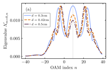
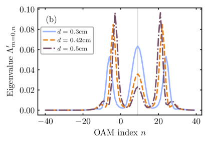
Refer to caption
((a))
Refer to caption
((b))
Figure 17: Cuts of the normalized modal weights Λm=0,nsubscriptsuperscriptΛ𝑚0𝑛\Lambda^{\prime}_{m=0,n} (m,nΛmn=1subscript𝑚𝑛subscriptsuperscriptΛ𝑚𝑛1{\sum_{m,n}\Lambda^{\prime}_{mn}}=1) for lp=18subscript𝑙𝑝18l_{p}=18, mp=0subscript𝑚𝑝0m_{p}=0 for the (a) low-gain and (b) high-gain regime for different distances between the crystals around the dark fringe point. The thin gray lines indicate n=lp/2=9𝑛subscript𝑙𝑝29n=l_{p}/2=9. For the distance d=0.42 cm𝑑times0.42centimeterd=$0.42\text{\,}\mathrm{cm}$ the most populated OAM mode appears at n=22𝑛22n=22, which is higher than the pump OAM lp=18subscript𝑙𝑝18l_{p}=18. According to Eq. 2.40, the most populated OAM modes are strongly amplified in the high-gain regime, leading to a reshaping of the eigenvalue spectrum [11].

Figure 17 shows the normalised (m,nΛmn=1subscript𝑚𝑛subscriptsuperscriptΛ𝑚𝑛1{\sum_{m,n}\Lambda^{\prime}_{mn}}=1) modal weights according to Eq. 2.40 for lp=18subscript𝑙𝑝18l_{p}=18, mp=0subscript𝑚𝑝0m_{p}=0 for the low-gain [Fig. 17(a)] and high-gain [Fig. 17(b)] regime for different distances between the crystals around the dark fringe point. In contrast to the case lp=7subscript𝑙𝑝7l_{p}=7 and mp=0subscript𝑚𝑝0m_{p}=0 which was presented in Sec. III.2 in Fig. 6, where we have found the highest populated mode n=11𝑛11n=11 for the distances d=0.42 cm𝑑times0.42centimeterd=$0.42\text{\,}\mathrm{cm}$ and d=0.5 cm𝑑times0.5centimeterd=$0.5\text{\,}\mathrm{cm}$, the highest populated modes we have found here for the case of lp=18subscript𝑙𝑝18l_{p}=18 and mp=0subscript𝑚𝑝0m_{p}=0 is n=22𝑛22n=22 for the distance d=0.42 cm𝑑times0.42centimeterd=$0.42\text{\,}\mathrm{cm}$ and n=21𝑛21n=21 for d=0.5 cm𝑑times0.5centimeterd=$0.5\text{\,}\mathrm{cm}$. Also, in this case, the highest populated mode has a higher OAM than the pump OAM (lp=18subscript𝑙𝑝18l_{p}=18).

References