High Frequency Matters: Uncertainty Guided Image Compression with Wavelet Diffusion
Abstract
Diffusion probabilistic models have recently achieved remarkable success in generating high-quality images. However, balancing high perceptual quality and low distortion remains challenging in image compression applications. To address this, we propose an efficient Uncertainty-Guided image compression approach with wavelet Diffusion (UGDiff). Our approach focuses on high frequency compression via the wavelet transform, since high frequency components are crucial for reconstructing image details. We introduce a wavelet conditional diffusion model for high frequency prediction, followed by a residual codec that compresses and transmits prediction residuals to the decoder. This diffusion prediction-then-residual compression paradigm effectively addresses the low fidelity issue common in direct reconstructions by existing diffusion models. Considering the uncertainty from the random sampling of the diffusion model, we further design an uncertainty-weighted rate-distortion (R-D) loss tailored for residual compression, providing a more rational trade-off between rate and distortion. Comprehensive experiments on two benchmark datasets validate the effectiveness of UGDiff, surpassing state-of-the-art image compression methods in R-D performance, perceptual quality, subjective quality, and inference time. Our code is available at: https://github.com/hejiaxiang1/Wavelet-Diffusion/tree/main.
Index Terms:
learned image compression, wavelet transform, diffusion model, uncertainty weighted rate-distortion loss.I Introduction
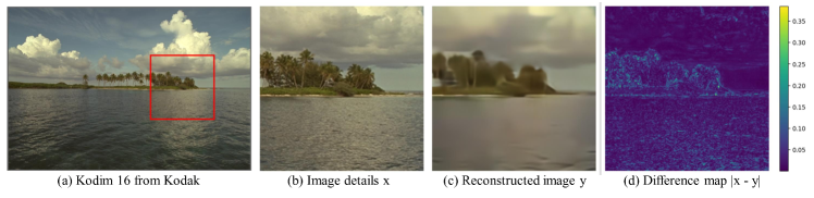
Given the exponential growth of media data, lossy image compression plays a crucial role in efficient storage and transmission. Established lossy image compression standards, such as JPEG [1], JPEG2000 [2], BPG [3], and VVC [4], follow a sequential paradigm of transformation, quantization, and entropy coding. Each stage is separately optimized with hand-crafted rules, making it challenging to adapt to diverse image content. Recently, learned image compression methods [5, 6, 7, 8] based on the variational auto-encoder (VAE) [9] have demonstrated superior rate-distortion performance compared to traditional techniques. Despite these advancements, these models often directly optimize for low distortion in terms of mean squared error (MSE), leading to a degradation in perceptual quality. This degradation typically manifests as over-smoothness or blurring, which has minimal impact on distortion metrics but adversely affects visual perception. As illustrated in Fig.1, high frequency details like textures and edges (e.g., trees and ripples) contain more significant visual information than smooth areas (e.g., sky). These regions with high frequency details often suffer severe distortion during compression, highlighting the need for improved methods that balance rate-distortion performance with perceptual quality.
A recent class of generative models focuses on improving the perceptual quality of reconstructions. Agustsson et al. [10] and Mentzer et al. [11] employed Generative Adversarial Networks (GANs) [12] as image decoders to generate reconstructions with rich details, albeit at the cost of some fidelity to the original image. Given the recent success of diffusion based models in image restoration tasks such as super-resolution [13, 14], deblurring [15] and inpainting [16, 17], Yang et al. [18] and Ghouse et al [19] leveraged diffusion models for image compression, achieving impressive results in terms of perception. However, it has been observed that vanilla diffusion models tend to reconstruct images with richer visual details but less fidelity to the original images. These models are prone to generate images with color distortion or artifacts due to the reverse process starting from randomly sampled Gaussian noise. This inherent uncertainty reveals the instability of reconstructed pixels, which is closely related to the fidelity of texture and edge recovery. Therefore, considering uncertainty from the random sampling of the diffusion model is crucial for enhancing the robustness and reliability of compression models.
The central challenge in balancing low distortion and high perception quality lies in the reconstruction of high frequency details, such as edges and textures. Enhancing high frequency reconstruction is an nontrivial task because high frequency typically possesses less energy and are therefore more susceptible to distortion compared to low frequency. Motivated by these issues, we propose an Uncertainty-Guided image compression approach with wavelet Diffusion (UGDiff) to maintain high perceptual quality as well as low distortion. We employ a discrete wavelet transform (DWT) to the image, compressing low frequency and high frequency components separately. Our focus is on high frequency compression to recover crucial high frequency details, thereby improving overall reconstruction quality.
Specially, we propose a wavelet diffusion model to predict high frequency, followed by a residual compression module that compresses and transmits the prediction residuals between original and predicted high frequency. This diffusion prediction-then-residual compression paradigm is able to effectively address the low fidelity issue common in direct reconstructions by existing diffusion models. To facilitate high frequency prediction via wavelet conditional diffusion, we introduce a condition generation module to derive a strong condition from the reconstructed low frequency by leveraging the inter-band relations between low and high frequency components. The advantages of combination of the diffusion model with discrete wavelet transform (DWT) [20] are twofold. On the one hand, DWT provides a sparser representation that is easier for a network to learn compared to the pixel domain [21]. On the other hand, DWT reduces the image’s spatial size by a factor of four, in accordance with the Nyquist rule [22], thereby expediting the inference speed of the denoising function.
Diffusion models are susceptible to generating unexpected chaotic content due to the randomness of sampling from Gaussian noise. The impact of this uncertainty on compression has not been thoroughly considered, meaning that low distortion cannot always be guaranteed although high perceptual quality may be achieved. Large uncertainty in predicted high frequencies results in large residuals, consuming more bits compared to those with low uncertainty. Motivated by this, we propose a novel uncertainty-guided residual compression module. We initially estimate the aleatoric uncertainty of the predicted high frequency using Monte Carlo [23] sampling of the diffusion model. Subsequently, we design an uncertainty-weighted rate-distortion (R-D) loss tailored for residual compression. In addition to the hyper-parameter that balances the overall R-D level for the entire dataset, we introduce an uncertainty-related weight to the distortion terms to prioritize residuals with large uncertainty, thereby allocating more bits to them. The main contributions are:
-
•
We propose a wavelet diffusion based predictive coding for high frequency. Our diffusion prediction-then-residual compression paradigm effectively addresses the low fidelity issue stemming from the direct reconstruction of existing diffusion models. In addition, the combination of DWT and diffusion models can greatly expedite the inference of diffusion model.
-
•
We introduce a novel uncertainty guided residual compression module, in which an uncertainty weighted R-D loss is designed to prioritize residuals with high uncertainty and allocate more bits to them. Our proposed uncertainty weighted R-D loss provides more rational trade-off between rate and distortion.
-
•
Extensive experiments conducted on two benchmark datasets demonstrated that our proposed method achieves state-of-the-art performance on both distortion metrics and perceptual quality while offering prominent speed up compared to previous diffusion-based methods.
II Related Work
Learned Image Compression Learned image compression methods have demonstrated substantial advancements in network structure and entropy modeling, resulting in significant enhancements in compression performance. Ballé et al. [24] firstly proposed an end-to-end image compression model. Then they incorporated a hyper-prior to effectively capture spatial dependencies in the latent representation [5]. Moreover, Minnen et al. [25] designed a channel-wise auto-regressive entropy model to achieve parallel computing. Ali et al. [26] proposed a novel non-auto-regressive model substitution approach, which reduced spatial correlations among elements in latent space by introducing a correlation loss, thereby enhancing the balance between image compression performance and complexity. Besides, Liu et al. [8] constructed a mixed Transformer-CNN image compression model, combining the local modeling capabilities of CNN with the non-local modeling capabilities of Transformers. To achieve better perceptual quality which is closer to human perception, a series of methods leveraging generative models to build decoders are proposed.Agustsson et al [10] and Mentzer et al. [11] propose to employ GANs [12] to achieve high perception quality at the cost of some fidelity to the original image.
Diffusion Models for Image Compression Denoising diffusion models [27] have progressed rapidly to set state-of-the-art for many image restoration tasks such as super-resolution [13, 14], inpainting [16, 17], and deblurring [15]. Some researchers have also explored the application of diffusion models in the image compression community. Yang et al. [18] replaced the decoder network in the image compression process with a conditional diffusion model. Alternative approaches were introduced by [19, 28]. They initially optimized an auto-encoder for a rate-distortion loss and subsequently trained a conditional diffusion model on the output of the auto-encoder to enhance its perception quality. Pan et al. [29] introduced text embedding as a conditioning mechanism to guide the stable diffusion model in reconstructing the original image. However, diffusion models are prone to compromise fidelity although high perception quality is achieved when utilized as an image decoder.
Uncertainty in Bayesian Neural Networks The uncertainty in Bayesian Neural Networks can be roughly divided into two categories [30]. Epistemic uncertainty describes how much the model is uncertain about its predictions. Another type is aleatoric uncertainty which refers to noise inherent in observation data. Notably, the integration of uncertainty modeling into deep learning frameworks has enhanced the performance and resilience of deep networks across various computer vision tasks, including image segmentation [31], image super-resolution [32] and etc. Badrinarayanan et al. [31] incorporated uncertainty estimation into image segmentation tasks, leading to more reliable segmentation results, especially in ambiguous regions. Ning et al. [32] extended uncertainty modeling to image super-resolution, leveraging Bayesian estimation frameworks to model the variance of super-resolution results and achieve more accurate and consistent image enhancement. Zhang et al. [33] proposed a scalable image compression framework that integrates uncertainty modeling into the scalable reconstruction process. Chan et al. proposed Hyper-diffusion to accurately estimate epistemic and aleatoric uncertainty of the diffusion model with a single model [34]. Nevertheless, there are few works that have investigated the uncertainty of diffusion models in image compression to the best of our knowledge. In this paper, we explore the influence of uncertainty in R-D loss and design an uncertainty weighted R-D loss to guide the residual compression optimization.
III Proposed Method
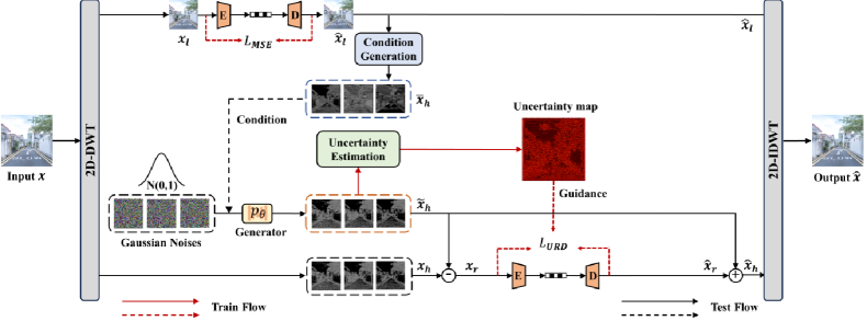
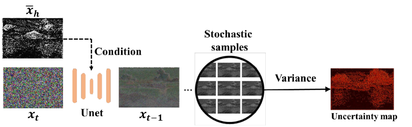
As illustrated in Fig.2, our proposed UGDiff follows a wavelet predictive coding paradigm, where low and high frequency components are compressed separately after DWT. The low frequency image is compressed by a pre-trained VAE based codec whose network structure is illustrated in the Appendix. Our work focuses on the high frequency compression to maintain high perception quality as well as low distortion. The condition generation module firstly generates refined high frequency from the reconstructed low frequency as the condition, which guides the wavelet diffusion to predict high frequency . The uncertainty map is simultaneously estimated upon the Monte Carlo Sampling during the reverse diffusion process. Then the residuals between original and predicted high frequency are compressed using another VAE based codec optimized by our proposed uncertainty weighted R-D loss in which the estimated uncertainty related weight is introduced to the distortion term to prioritize residuals with large uncertainty and allocate more bits to them. Finally, the reconstructed low and high frequency components are inversely transformed by 2D-IDWT (inverse DWT) to obtain reconstructed images.
III-A Wavelet Conditional Diffusion Model
With respect to image compression tasks, there are two challenges associated with the conditional diffusion model: 1) Small noise variance permits the assumption that the inverse denoising process approximates a Gaussian distribution. That results in large sampling steps (typically set to 500) and significant inference time [18]. 2) The diversity in the sampling process may introduce content inconsistency in the generation results, which makes application of diffusion models in image compression challenging.
To address these challenges, we propose a wavelet diffusion based predictive coding for high frequency. Our approach leverages the strength of wavelet transform to speed up the inference process of the diffusion model by quartering the spatial dimensions without sacrificing information. Different from the existing diffusion models to reconstruct the image directly, our approach utilize the diffusion model for high frequency prediction and follow a prediction residual codec to address the low fidelity issues.
Discrete Wavelet Transform 2D-DWT employs a convolutional and sub-sampling operator, denoted as , to transform images from spatial domain to frequency domain, thus enabling the diffusion process solely on high frequency components. Let denote an original-reconstruction image pair. Before applying the diffusion process, the specific wavelet operator , such as haar wavelet [35], decomposes into its low frequency component and an array of high frequency components . Mathematically, this can be represented as:
| (1) |
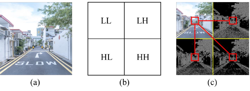
2D-DWT decomposes the image into four sub-bands, namely, Low Low (LL), Low High (LH), High Low (HL) and High High (HH). The subband LL represents the low frequency component that contains global information akin to a down-sampled version of the image, while the remaining sub-bands, LH, HL and HH, represent the high frequency components that comprise sparse local details, as illustrated in Fig. 3.
By operating in the wavelet domain, we open the possibility for diffusion models to focus on isolated high frequency details, which is often lost when the data is processed directly. In addition, utilizing 2D-DWT allows for faster inference speed for diffusion models as the spatial size is quartered according to the Nyquist rule.
High Frequency Condition Generation The naive way to apply wavelet diffusion in high frequency prediction is to directly corrupt high frequency with additive Gaussian noise in the forward process and then learn to reverse it in the sampling phase, taking reconstructed low frequency as the condition to guide the reverse diffusion process, as the similar way in [36, 14]. Nonetheless, low frequency cannot guide the conditional diffusion to generate satisfactory predicted high frequency as expected, since utilizing the low frequency as the condition would enforce the diffusion model to generate an image that resembles low frequency rather than high frequency as will be illustrated in Fig.10.
To derive conditions that encapsulate high frequency details for wavelet diffusion, we investigate the correlation between the wavelet low frequency and high frequency sub-bands. We present the tree structure diagram of the wavelet decomposition to provide a clearer illustration of the sub-bands correlations in Fig.3. Inspired by the inter-band correlations of wavelet sub-bands, we design a high frequency condition generation module to convert the reconstructed low frequency into refined high frequency as the condition for wavelet conditional diffusion, i.e., ,where is a neural network described in the Appendix.
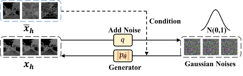
Conditional Diffusion Equipped with the refined high frequency as the condition , we design a conditional diffusion model in the frequency domain to generate predicted high frequency with high quality. A conditional Denoising Diffusion Probabilistic Model (DDPM) utilizes two Markov chains [27]. The first is a forward chain responsible for adding Gaussian noise to the data:
| (2) |
where represents a variance schedule.
The other Markov chain is a reverse chain that transforms noise back into the original data distribution. As is illustrated in Fig. 4, the key idea of our wavelet conditional diffusion is to introduce the refined high frequency as the condition into the diffusion model , thereby, becomes :
| (3) |
where represents conditional guidance that controls the reverse diffusion process. The parameters are typically optimized by a neural network that predicts of Gaussian distributions. This is simplified by predicting noise vectors with the following objective:
| (4) |
Subsequently, the sampling phase can commence with using the noise predicted from the learned neural network, as follows:
| (5) |
where , , and .
This iterative sampling process enables the generation of samples backward in time, where each sample is computed based on the previously generated sample . During the sampling process, the refined high frequency is embedded into each step of the reverse diffusion process, which makes the sampled image consistent with the distribution of and thus improves the quality of the predicted high frequency. The pseudo-code for sampling with conditional diffusion is as Alg.1.
III-B Uncertainty-guided Residual Compression
Diffusion models exhibits inherent uncertainty due to randomness of sampling from Gaussian noise, which will introduce instability in subsequent residual compression. Large uncertainty in predicted high frequency will produce large residuals that will consumes more bits than those with low uncertainty. A learned image compression model aims to optimize the R-D loss so that the minimum distortion can be achieved with the minimum bitrate. Specifically, a trade-off hyper-parameter is utilized to balance the rate and distortion that is applied to the entire dataset, whereas the uncertainty within one image is not considered in this global trade-off.
To alleviate the influence of uncertainty from the diffusion prediction on the subsequent residual compression, we propose an uncertainty-guided residual compression module. Firstly, the aleatoric uncertainty of the predicted high frequency is estimated upon the Monte Carlo sampling [23] of the above diffusion model. Subsequently, a novel uncertainty weighted R-D loss is designed in which the aleatoric uncertainty map is incorporated to prioritize pixels with high uncertainty and dynamically allocate more bits to them than those with low uncertainty. The introduction of uncertainty allows for more rational trade-off between rate and distortion considering the disequilibrium of the residuals, ultimately leading to improved compression performance.
Uncertainty estimation. Aleatoric uncertainty arises from inherent variability and randomness in the underlying processes being modeled. Unlike other deterministic neural networks relying on Monte Carlo dropout mechanisms [37], uncertainty estimation of the diffusion model is conceptually straightforward due to the randomness of the input noise. To be specific, aleatoric uncertainty can be captured by the variance of samples generated by a diffusion model.
The uncertain estimation details are illustrated in Fig.5. For a given conditional input , our wavelet conditional diffusion model yields different prediction samples of high frequency outputs after times Monte Carlo Sampling, where denotes the prediction obtained from the k-th sampling given different initial input noise. To obtain an estimate of uncertainty regarding the high frequency predictions, the mean and variance of these predictions is computed. The predicted mean of the output is calculated as:
| (6) |
The uncertainty of the prediction can be quantified by the variance of the prediction results, given by:
| (7) |
Here, represents the predicted mean, and denotes the predicted variance, which serves as an estimate of the uncertainty associated with the prediction results.
Uncertainty weighted R-D Loss. Given an arbitrary image , optimizing the VAE based image compression model for R–D performance has been proven to be equivalent to minimization of the KL divergence by matching the parametric density functions to the transform coding framework as follows [5],
| (8) | ||||
where is an approximation to the quantized latent representations with an additive i.i.d. uniform noise to enable end-to-end training.
Specifically, minimizing log likelihood in the KL divergence is equivalent to minimizing the distortion between original and reconstructed measured by squared difference when the likelihood . The second term in Eq.(8) denotes the cross entropy that reflects the cost of encoding i.e., bitrate . The R-D loss can be reformulated as
| (9) |
where is a hyper-parameter used to balance the overall rate-distortion, i.e.,larger for larger rate and better reconstruction quality and vice versa. is a global hyper-parameter applied to the entire dataset, whereas the uncertainty within one image is neglected in this trade-off.
To address this issue, we reconsider the weighted R-D loss with aleatoric uncertainty. Let represent the residuals to be compressed, represents the variational inference in residual compression module, denotes the aleatoric uncertainty estimated in the above subsection. This way, the compression model can be formulated as:
| (10) |
where represents the Gaussian distribution with zero-mean and unit-variance, which is assumed for characterizing the likelihood function by:
| (11) |
Then a negative log likelihood then works out to be the uncertainty weighted distortion term between and ,
| (12) |
Uncertainty is incorporated into the denominator of the distortion term, resulting in residuals with high uncertainty having a relatively minor impact on the overall R-D loss function. Through comparison with the distortion term in Eq.(9), we find that the weights and play the same role in the the distortion term. They both penalize pixels with large variance. However, in contrast to the role of the hyperparameter in balancing the rate-distortion trade-off, the uncertainty, which serves as the prior of the image to be encoded, indicates pixels with high uncertainty requires a greater allocation of bits compared to those with low uncertainty.
Inspired by that, we propose a new adaptive weighted loss named uncertainty-weighted rate-distortion loss () for residual compression. Actually, we need a monotonically increasing function to prioritize pixels with large uncertainty rather than penalize them using .
Differential entropy is a measure of the information content of a continuous random variable, which reflects the cost of coding. The differential entropy of the random variable is computed as follows given the probability density function .
| (13) |
We substitute the probability distribution in Eq.(11) into Eq.(13) to obtain the differential entropy of ,
| (14) |
Eq.(14) demonstrates the increase trend of differential entropy with the variance . Motivated by this equation, we use the weight to prioritize pixels with large uncertainty in the R-D loss function. Combining the hyper-parameter to balance the overall trade-off between the rate and distortion, the uncertainty weighted R-D loss function is reformulated as:
| (15) |
where serves as a global weight applied to the entire dataset to balance the rate and distortion, whereas estimated uncertainty serves as a regulator within the image to prioritize pixels with large uncertainty and allocate more bits to them during compression. Our proposed uncertainty weighted R-D loss provides more rational trade-off between the rate and distortion compared with the regular R-D loss without uncertainty.
III-C Training Strategy
As the analysis above, the whole training process of UGDiff contains four steps. Firstly, we train a learned image compression network [25] for our low frequency codec. Details of the network structure is shown in Appendix. The loss function is
| (16) | ||||
where controls the trade-off between rate and distortion. R represents the bit rate of latent and side information , and is the MSE distortion term.
The second step is to train the condition generation module, aiming at converting reconstructed low frequency to refined high frequency condition . We employed a deep convolutional neural network with localized receptive fields, whose structure is illustrated in Appendix, optimized by minimizing MSE between the output and the original high frequency,
| (17) |
The third step is to train the conditional diffusion model. The design of the denoising network in the diffusion model follows a similar U-Net architecture used in DDPM [27] enhanced with residual convolutional blocks[38] and self-attention mechanisms.We use Eq.(4) to optimize the parameters of the denoising network.
The final step is to train the uncertainty guided residual compression model. The residual compression model follows the same structure as that for the low frequency compression, while optimized to minimize the uncertainty weighted R-D loss in Eq.(15).
IV Experiment
IV-A Implement Details
Training. We use the OpenImages dataset [39] to train our models, consisting of over 9 million images. This dataset is widely used for image compression research. We randomly selected 300k images from OpenImages, resized them to 256 × 256 in each epoch. All models were trained using the Adam optimizer [40] for 1.8 million steps with a batch size of 16. The initial learning rate was set to for the first 120k iterations, then reduced to for the following 30k iterations, and further decreased to for the last 30k iterations. We configured the within the range 0.01, 0.05, 0.1, 0.2, 0.3 for MSE optimization of low frequency compression network and residual compression module. Additionally, we maintained consistency in the number of channels, setting N = 192 and M = 320 for all models. We conduct the experiments using the Pytorch [41] and CompressAI libraries [42] over one NVIDIA Geforce RTX4090 GPU with 24GB memory.
Evaluation. The evaluations are conducted on the Kodak dataset [43] and Tecnick dataset [44]. The Kodak dataset comprises 24 images with a resolution of 768x512 pixels. The Tecnick dataset includes 100 natural images with 600x600 resolutions. We calculate bit-per-pixel (bpp) for each image to show bitrate. We reach different ranges of bitrates by compressing images with different models trained using different . For reconstruction distortion, the common PSNR and MS-SSIM [45] are evaluated for all models. PSNR represents the pixel-level distortion while MS-SSIM describes the structural similarity. In addition, we also compute the Learned Perceptual Image Patch Similarity (LPIPS) metric [46] to evaluate the perception loss.
IV-B Comparison with the SOTA Methods
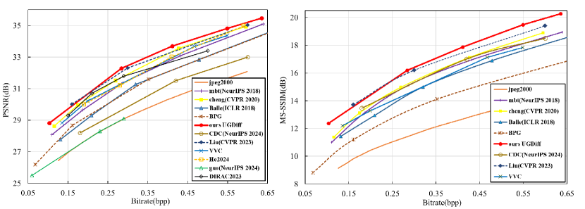
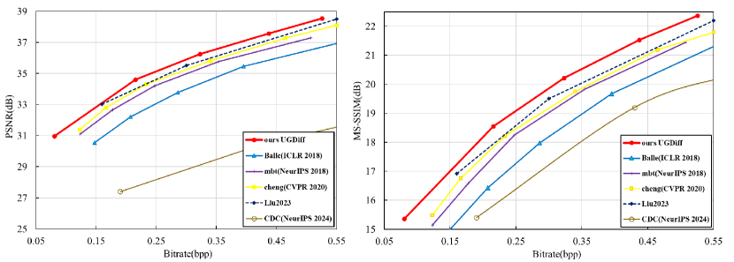
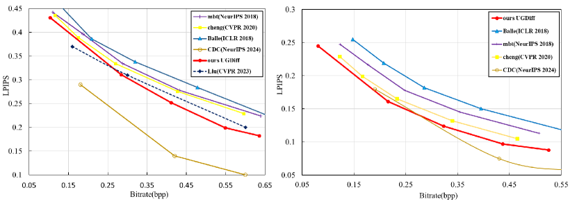
Rate-Distortion Performance. To show the effectiveness of our UGDiff, we compare its R-D performance with the state-of-the-art (SOTA) image compression methods including diffusion model-based compression methods, such as CDC NeurIPS2024 () [18],DIRAC(single sampling step is adopted to achieve minimal distortion) [19], learned image compression methods, as well as traditional compression standards. The traditional compression standards include JPEG2000 [2], BPG [3], and VVC [4]. The learned compression methods include the context-free hyperprior model (Balle ICLR2018) [5], the auto-regressive hyperprior models (mbt NeurIPS2018) [6], entropy models with Gaussian Mixture Models and simplified attention (Cheng CVPR2020) [7], Mixed Transformer-CNN model (Liu CVPR2023) [8], lightweight attention model(He ESA2024) [47] and implicit neural representation model (Guo2024 NeurIPS 2024) [48].
Fig.6 and Fig.7 compare R-D curves in terms of PSNR and MS-SSIM verus bitrates averaged over the Kodak and Technick datasets respectively. Fig.8 compares the perception performance of different compression methods in terms of LPIPS over the Kodak and Technick datasets respectively. The figures demonstrate that our proposed UGDiff significantly outperforms SOTA compression methods including traditional codec, learned image compression methods as well as other diffusion based methods at all bitrate points in terms of PSNR, MS-SSIM, especially at low bitrates. The diffusion based methods, such as CDC, achieve excellent perception quality in terms of LPIPS ,whereas the fidelity is compromised resulting in inferiority to other learned image compression approaches in terms of PSNR and MS-SSIM. The experimental results demonstrate that our proposed UGDiff achieves better trade-off between perception and distortion metric compared to other diffusion methods. The reasons are twofold. Firstly, we utilized a novel diffusion predict-then-residual compress paradigm to address low fidelity issues during direct reconstruction from the diffusion model. Secondly, the uncertainty stemming from random sampling in diffusion is considered in the residual compression to achieve more rational trade-off between rate and distortion.
BD-rate Analysis. To further compare the R-D performance quantitatively, we use the Bjøntegaard-delta-rate(BD-rate) metric [49] to compute the average bitrate savings for the same reconstruction quality in terms of PSNR. We use VVC intra [4] (version 12.1), the current best hand crafted codec, as the anchor to compute BD-rate. The BD-rates are shown in Table.I. It is evident that our UGDiff outperforms the current best traditional codecs VVC, achieving the BD-rate savings of 8.02% and 11.54% on Kodak and Tecnick datasets respectively. And compared with the SOTA learned image Compression method Liu’2023, our UGDiff still achieves the BD-rate savings of 0.64% and 1.51%. Notably, our UGDiff achieves the Bd-rate savings of 23.66% and 31.13% compared with the diffusion based approach CDC, which demonstrates great improvement in terms of distortion metric. These comparisons demonstrate the RD performance superiority of our UGDiff over SOTA image compression methods.
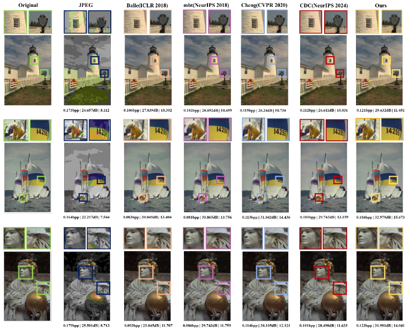
Subjective Quality Comparison. We also implement subjective quality evaluations on Kodak dataset. Fig. 9 presents visual comparisons for original images along with the corresponding reconstructed results produced by various compression methods. As is shown in the second column of Fig.9, JPEG produces severe blocking effects due to the partitioning mechanism in the coding standards. The learned image compression methods,such as Balle’2018, Cheng’2020, suffer from over-smoothing issues, characterized by a loss of textural fidelity in the reconstructed images. In particular, the subtle smile in the sign board within the first image are diminished,the numerals within the blue expanse of the sail in the second image are obscured, and the facial features of the statue in the third image are rendered with an excessive degree of smoothness. our proposed UGDiff retains more high frequency details and exhibits superior subjective visual qualities. The details are still perceptible in our reconstructed images,such as the smiling faces on the signboards, the numerals on the blue sail, and the cavities on the face of the statue.
Complexity Analysis. We also evaluate the complexity by comparing the inference time of different compression methods on the Kodak dataset with the size of 512×768. Here, we calculate the encoding time and decoding time at the similar R-D points to evaluate the model complexity. For fair comparison, all the models are implemented on the same GPU using their public codes. It can be observed from Table.II, that Balle’2018 demonstrates the lowest model complexity among the learned image codec. The diffusion model CDC suffers from slow decoding speed due to their iterative denoising process (A default sampling step 500 is adopted). Specifically, it takes approximately 55s to decode an image. Benefiting from the proposed wavelet diffusion model only implemented on sparse high frequency components, our UGDiff is at least 40× faster than CDC (A sampling step 10 is needed). Specifically the decoding time of our UGDiff can be reduced from 55s to 1.47s with a even higher PSNR compared with CDC.
IV-C Ablation Studies
We conduct the ablation studies to further analyze our proposed UGDiff. Firstly, we evaluate the sampling steps in the reverse denoising process. Then, we conduct ablation studies through including or excluding the components to evaluate the effect of high frequency, wavelet diffusion, diffusion condition as well as the uncertainty guidance. The specific components encompasses the low frequency codec, condition generation, wavelet diffusion, residual codec and uncertainty map guidance.
Sampling steps. A factor that determines the inference speed of the diffusion models is the sampling step used in the reverse denoising process. We conducted an ablation study of various settings of diffusion models on the condition and sampling step in Table.IV. The table clearly demonstrates that the R-D performance approaches a state of saturation when the sampling step exceeds a threshold of 10 irrespective of the guiding condition employed in the diffusion process, whether it be or . By contrast, large sampling step is essential for CDC 2024 to generate images with the best perception quality. Compared with CDC 2024 that employed the diffusion in the pixel domain, the inference speed of our UGDiff is accelerated through two key factors: the spatial dimension is quartered by 2D-DWT, in addition, high frequency contains more sparse information in the frequency domain compared to the image domain.
Effect of high frequency. We conduct an ablation study to validate the effectiveness of the high frequency on the image compression performance. We conduct comparative experiments using 3 variants. Variant 1:Without high frequency. Only low frequency is compressed and transmitted to the decoder to reconstruct the image without high frequency. The R-D performance is shown in the 1st column. Variant 2: Predict high frequency. Only low frequency is compressed and transmitted to the decoder, meanwhile, the high frequency is predicted from the reconstructed low frequency at the decoder. The R-D performance is demonstrated in the 2nd and 3rd columns utilizing condition generation and wavelet diffusion for prediction respectively. Variant 3:Reconstruct high frequency. Besides the low frequency, the residual between original and predicted high frequency is also compressed and transmitted to the decoder. The high frequency is reconstructed by adding the reconstructed residual and the predicted high frequency. The R-D performance is shown in the 4th and 5th columns utilizing condition generation and wavelet diffusion for prediction respectively.
| Component | Choice | |||||
| Low frequency codec | ✓ | ✓ | ✓ | ✓ | ✓ | |
| Condition generation | ✓ | ✓ | ✓ | ✓ | ||
| Wavelet diffusion | ✓ | ✓ | ||||
| Residual codec | ✓ | ✓ | ||||
| bitrate(bpp) | 0.21 | 0.21 | 0.21 | 0.24 | 0.23 | |
| PSNR(dB) | 27.88 | 28.24 | 28.96 | 31.02 | 31.33 | |
| MS-SSIM(dB) | 14.66 | 15.05 | 15.27 | 15.53 | 15.78 |
From the results demonstrated in Table. III, we can observe that high frequency contributes dramatic performance gains although very few bits are consumed. When high frequency is discarded while only low frequency is transmitted, the RD performance drops dramatically. By comparing the 1st column with the 2nd and 3rd columns, we can observe that the high frequency components, which are merely predicted from the reconstructed low frequency without any additional bit consumption, yields a PSNR improvement ranging from 0.4 to 1.0 dB depending upon the prediction mechanism employed . Even the most accurate prediction values exhibit discrepancies when compared to their original counterparts. By comparing 2nd, 3rd and the 4th, 5th columns in the table, substantial PSNR improvement of about 2.5dB is further achieved with a minimal increase in bit consumption when the residual between original and predicted high frequency is also compressed and transmitted to the decoder to facilitate high frequency reconstruction. In conclusion, high frequency play a pivotal rule in image conclusion, which motivates us to focus on high frequency compression.
Effect of Wavelet Diffusion. To validate the effectiveness of wavelet diffusion on the image compression performance, we conduct an ablation study using 3 variants. Variant 1: Without wavelet diffusion. The refined high frequency obtained by the condition generation module are directly used for high frequency reconstruction without reverse diffusion sampling, whose R-D performance is shown at the 2nd column of the Table. III. Variant 2: Utilizing Wavelet Diffusion for reconstruction. High frequency is generated from the wavelet diffusion model guided by the refined high frequency derived from the condition generation module, whose R-D performance is shown at the 3rd column of Table. III. Variant 3:Utilizing Wavelet diffusion for prediction. High frequency is predicted from the wavelet diffusion, and the prediction residual between the original and predicted high frequency is also compressed and transmitted to the decoder, whose R-D performance is shown at the 5th column of Table. III.
By comparing the variants with and without wavelet diffusion in the 2nd and 3rd columns in the table, we observe that wavelet diffusion greatly improves the image compression performance due to its great capacity to generate images. When wavelet diffusion is utilized to reconstruct high frequency directly, PSNR is improved by 0.72dB compared with that without wavelet diffusion. Further more, When wavelet diffusion is utilized to predict high frequency and the prediction residual is also transmitted, the PSNR is further improved by 2.37dB comparing variant 2 in the 3rd column with variant 3 in the 5th column. That is mainly because the diffusion models may compromise fidelity when applied to reconstruct images directly. Therefore, prediction is a more suitable strategy than direct reconstruction when the diffusion model is applied to image compression.
Effect of Condition on Diffusion. The condition controls the generation content of the diffusion model tightly. We introduced a condition generation module which obtains a condition stronger than the reconstructed low frequency by leveraging the inter-band correlation of wavelet coefficients. To conduct an ablation study which validates the effectiveness of the condition generation module, we implement a baseline by using the reconstructed low frequency as the condition directly without condition generation. Table.IV compares the overall R-D performance of our proposed UGDiff under different conditions and sampling steps. Compared with that conditioned by reconstructed low frequency, about 0.3dB improvement regarding PSNR and 1.25dB improvement regarding MS-SSIM are achieved by UGDiff conditioned by the refined high frequency obtained by the condition generation module.
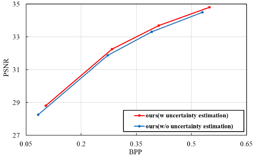
Effect of Uncertainty Guidance. We conduct an ablation study to evaluate the effect of uncertainty guidance on our UGDiff. Fig.11 compares the R-D curves of variants with and without uncertainty estimation. From the figure we can observe R-D performance gains at all R-D points when the uncertainty of diffusion model is introduced in the weighted R-D loss to optimize the residual compression model.
IV-D Further Analysis
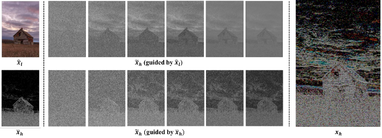
Wavelet diffusion condition. The guiding condition exerts strong control over the reverse diffusion process. Fig.10 illustrates the visualization results of reverse diffusion process under different conditions. From the first row of the figure, it is evident that the process of reverse diffusion, when conditioned by the reconstructed low frequency , leads to acquisition of an image that resembles low frequency representation, consequently manifesting a loss of certain detailed textures. That would make the prediction residual quite large and affect the efficacy of residual compression. As is illustrated in the figure, the generated refined high frequency from the condition generation module contains more high frequency details. The visualization of reverse diffusion process demonstrates that the generated image sampled from reverse diffusion conditioned by refined high frequency resembles original high frequency more than that conditioned by low frequency. That indicates our proposed condition generation module can provide a strong guide for the conditional diffusion model to predict high frequency.
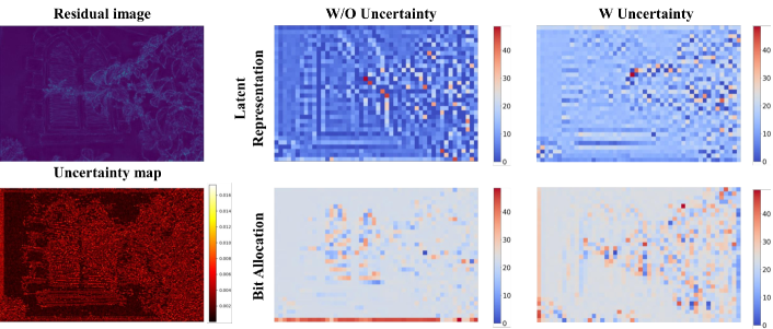
Uncertainty weighted rate-distortion loss. To thoroughly investigate the impact of uncertainty weighted rate-distortion loss on residual compression networks, we visually illustrate the residual image, uncertainty map, latent representations, and bit allocation of models with and without uncertainty-guided optimization respectively in Fig.12. The figure demonstrates that the distribution of predictive residuals is found to be consistent with the distribution delineated in the uncertainty map, which demonstrates that the uncertainty map reveals instability of the wavelet diffusion model to predict the high frequency. Furthermore, it is observed in the 2nd column that the residual compression model, which employ a regular rate-distortion loss neglecting uncertainty, treats residuals more uniformly and allocates bits more evenly across the entire residual image. By contrast, the uncertainty weighted rate-distortion loss enforces the residual compression network to prioritize the large residuals identified by the uncertainty map. Consequently, the latent representations of these regions become more prominent, leading to more rational bit allocations.
V Conclusion
In this paper, we present an effective Uncertainty Guided image compression approach with wavelet Diffusion (UGDiff). We employ the wavelet diffusion for high frequency prediction rather than direct reconstruction and subsequently utilize a residual compression module to maximally recover high frequency details. This diffusion prediction-then-residual compression paradigm effectively addresses the low fidelity issue common in existing diffusion models. In addition, our wavelet diffusion approach exhibits a significant improvement in inference speed compared to previous diffusion-based methods. We also designed an uncertainty weighted R-D loss for the residual compression module, which provide more rational trade-off between the bitrate and distortion. Experimental results demonstrate that our proposed UGDiff outperforms state-of-the-art learned image compression methods in terms of R-D performance and subjective visual quality. Considering the great capacity of wavelet transform in multi-resolution analysis, we plan to extend our approach to resolution scalable image compression in our future work.
Acknowledgments
This work was supported in part by the National Natural Science Foundation of China under Grant 62373293. Professor Ajmal Mian is the recipient of an Australian Research Council Future Fellowship Award (project number FT210100268) funded by the Australian Government.
References
- [1] G. K. Wallace, “The jpeg still picture compression standard,” IEEE transactions on consumer electronics, vol. 38, no. 1, pp. xviii–xxxiv, 1992.
- [2] D. S. Taubman, M. W. Marcellin, and M. Rabbani, “Jpeg2000: Image compression fundamentals, standards and practice,” Journal of Electronic Imaging, vol. 11, no. 2, pp. 286–287, 2002.
- [3] F. Bellard, “Bpg image format,” https://bellard.org/bpg/, 2018.
- [4] J. V. E. Team, “Vvc official test model vtm,” https://jvet.hhi.fraunhofer.de/, 2021.
- [5] J. Ballé, D. Minnen, S. Singh, S. J. Hwang, and N. Johnston, “Variational image compression with a scale hyperprior,” in International Conference on Learning Representations, 2018.
- [6] D. Minnen, J. Ballé, and G. Toderici, “Joint autoregressive and hierarchical priors for learned image compression,” in Proceedings of the 32nd International Conference on Neural Information Processing Systems, 2018, pp. 10 794–10 803.
- [7] Z. Cheng, H. Sun, M. Takeuchi, and J. Katto, “Learned image compression with discretized gaussian mixture likelihoods and attention modules,” in Proceedings of the IEEE/CVF conference on computer vision and pattern recognition, 2020, pp. 7939–7948.
- [8] J. Liu, H. Sun, and J. Katto, “Learned image compression with mixed transformer-cnn architectures,” in Proceedings of the IEEE/CVF Conference on Computer Vision and Pattern Recognition, 2023, pp. 14 388–14 397.
- [9] D. P. Kingma and M. Welling, “Auto-encoding variational bayes,” arXiv.org, 2014.
- [10] E. Agustsson, D. Minnen, G. Toderici, and F. Mentzer, “Multi-realism image compression with a conditional generator,” in Proceedings of the IEEE/CVF Conference on Computer Vision and Pattern Recognition, 2023, pp. 22 324–22 333.
- [11] F. Mentzer, G. D. Toderici, M. Tschannen, and E. Agustsson, “High-fidelity generative image compression,” Advances in Neural Information Processing Systems, vol. 33, pp. 11 913–11 924, 2020.
- [12] I. Goodfellow, J. Pouget-Abadie, M. Mirza, B. Xu, D. Warde-Farley, S. Ozair, A. Courville, and Y. Bengio, “Generative adversarial nets,” Advances in neural information processing systems, vol. 27, 2014.
- [13] C. Saharia, J. Ho, W. Chan, T. Salimans, D. J. Fleet, and M. Norouzi, “Image super-resolution via iterative refinement,” IEEE transactions on pattern analysis and machine intelligence, vol. 45, no. 4, pp. 4713–4726, 2022.
- [14] S. Shang, Z. Shan, G. Liu, L. Wang, X. Wang, Z. Zhang, and J. Zhang, “Resdiff: Combining cnn and diffusion model for image super-resolution,” in Proceedings of the AAAI Conference on Artificial Intelligence, vol. 38, no. 8, 2024, pp. 8975–8983.
- [15] J. Whang, M. Delbracio, H. Talebi, C. Saharia, A. G. Dimakis, and P. Milanfar, “Deblurring via stochastic refinement,” in Proceedings of the IEEE/CVF Conference on Computer Vision and Pattern Recognition, 2022, pp. 16 293–16 303.
- [16] C. Saharia, W. Chan, H. Chang, C. Lee, J. Ho, T. Salimans, D. Fleet, and M. Norouzi, “Palette: Image-to-image diffusion models,” in ACM SIGGRAPH 2022 conference proceedings, 2022, pp. 1–10.
- [17] A. Lugmayr, M. Danelljan, A. Romero, F. Yu, R. Timofte, and L. Van Gool, “Repaint: Inpainting using denoising diffusion probabilistic models,” in Proceedings of the IEEE/CVF Conference on Computer Vision and Pattern Recognition, 2022, pp. 11 461–11 471.
- [18] R. Yang and S. Mandt, “Lossy image compression with conditional diffusion models,” Advances in Neural Information Processing Systems, vol. 36, 2024.
- [19] N. F. Ghouse, J. Petersen, A. Wiggers, T. Xu, and G. Sautiere, “A residual diffusion model for high perceptual quality codec augmentation,” arXiv preprint arXiv:2301.05489, 2023.
- [20] S. Mallat, A wavelet tour of signal processing. Elsevier, 1999.
- [21] B. Moser, S. Frolov, F. Raue, S. Palacio, and A. Dengel, “Waving goodbye to low-res: A diffusion-wavelet approach for image super-resolution,” arXiv preprint arXiv:2304.01994, 2023.
- [22] H. Landau, “Sampling, data transmission, and the nyquist rate,” Proceedings of the IEEE, vol. 55, no. 10, pp. 1701–1706, 1967.
- [23] L. Acerbi, “Variational bayesian monte carlo,” Advances in Neural Information Processing Systems, vol. 31, 2018.
- [24] J. Ballé, V. Laparra, and E. P. Simoncelli, “End-to-end optimized image compression,” arXiv preprint arXiv:1611.01704, 2016.
- [25] D. Minnen and S. Singh, “Channel-wise autoregressive entropy models for learned image compression,” in 2020 IEEE International Conference on Image Processing (ICIP). IEEE, 2020, pp. 3339–3343.
- [26] Z. Li, Y. Zhou, H. Wei, C. Ge, and J. Jiang, “Towards extreme image compression with latent feature guidance and diffusion prior,” arXiv preprint arXiv:2404.18820, 2024.
- [27] J. Ho, A. Jain, and P. Abbeel, “Denoising diffusion probabilistic models,” Advances in neural information processing systems, vol. 33, pp. 6840–6851, 2020.
- [28] E. Hoogeboom, E. Agustsson, F. Mentzer, L. Versari, G. Toderici, and L. Theis, “High-fidelity image compression with score-based generative models,” arXiv preprint arXiv:2305.18231, 2023.
- [29] Z. Pan, X. Zhou, and H. Tian, “Extreme generative image compression by learning text embedding from diffusion models,” arXiv preprint arXiv:2211.07793, 2022.
- [30] A. Der Kiureghian and O. Ditlevsen, “Aleatory or epistemic? does it matter?” Structural safety, vol. 31, no. 2, pp. 105–112, 2009.
- [31] V. Badrinarayanan, A. Kendall, and R. Cipolla, “Segnet: A deep convolutional encoder-decoder architecture for image segmentation,” IEEE transactions on pattern analysis and machine intelligence, vol. 39, no. 12, pp. 2481–2495, 2017.
- [32] Q. Ning, W. Dong, X. Li, J. Wu, and G. Shi, “Uncertainty-driven loss for single image super-resolution,” Advances in Neural Information Processing Systems, vol. 34, pp. 16 398–16 409, 2021.
- [33] D. Zhang, F. Li, M. Liu, R. Cong, H. Bai, M. Wang, and Y. Zhao, “Exploring resolution fields for scalable image compression with uncertainty guidance,” IEEE Transactions on Circuits and Systems for Video Technology, 2023.
- [34] M. A. Chan, M. J. Molina, and C. A. Metzler, “Hyper-diffusion: Estimating epistemic and aleatoric uncertainty with a single model,” arXiv preprint arXiv:2402.03478, 2024.
- [35] A. Haar, “Zur theorie der orthogonalen funktionensysteme. (erste mitteilung).” Mathematische Annalen, vol. 69, pp. 331–371, 1910. [Online]. Available: http://eudml.org/doc/158469
- [36] H. Jiang, A. Luo, H. Fan, S. Han, and S. Liu, “Low-light image enhancement with wavelet-based diffusion models,” ACM Transactions on Graphics (TOG), vol. 42, no. 6, pp. 1–14, 2023.
- [37] Y. Gal and Z. Ghahramani, “Dropout as a bayesian approximation: Representing model uncertainty in deep learning,” in international conference on machine learning. PMLR, 2016, pp. 1050–1059.
- [38] K. He, X. Zhang, S. Ren, and J. Sun, “Deep residual learning for image recognition,” in Proceedings of the IEEE Conference on Computer Vision and Pattern Recognition (CVPR), June 2016.
- [39] I. Krasin, T. Duerig, N. Alldrin, V. Ferrari, S. Abu-El-Haija, A. Kuznetsova, H. Rom, J. Uijlings, S. Popov, A. Veit, S. Belongie, V. Gomes, A. Gupta, C. Sun, G. Chechik, D. Cai, Z. Feng, D. Narayanan, and K. Murphy, “Openimages: A public dataset for large-scale multi-label and multi-class image classification.” Dataset available from https://github.com/openimages, 2017.
- [40] D. Kingma and J. Ba, “Adam: A method for stochastic optimization,” in International Conference on Learning Representations (ICLR), San Diega, CA, USA, 2015.
- [41] A. Paszke, S. Gross, F. Massa, A. Lerer, J. Bradbury, G. Chanan, T. Killeen, Z. Lin, N. Gimelshein, L. Antiga et al., “Pytorch: An imperative style, high-performance deep learning library,” Advances in neural information processing systems, vol. 32, 2019.
- [42] J. Bégaint, F. Racapé, S. Feltman, and A. Pushparaja, “Compressai: a pytorch library and evaluation platform for end-to-end compression research,” arXiv preprint arXiv:2011.03029, 2020.
- [43] R. Franzen, “Kodak lossless true color image suite,” source: http://r0k. us/graphics/kodak, vol. 4, no. 2, p. 9, 1999.
- [44] N. Asuni and A. Giachetti, “TESTIMAGES: a Large-scale Archive for Testing Visual Devices and Basic Image Processing Algorithms,” in Smart Tools and Apps for Graphics - Eurographics Italian Chapter Conference, A. Giachetti, Ed. The Eurographics Association, 2014.
- [45] Z. Wang, E. Simoncelli, and A. Bovik, “Multiscale structural similarity for image quality assessment,” in The Thrity-Seventh Asilomar Conference on Signals, Systems & Computers, 2003, vol. 2, 2003, pp. 1398–1402 Vol.2.
- [46] R. Zhang, P. Isola, A. A. Efros, E. Shechtman, and O. Wang, “The unreasonable effectiveness of deep features as a perceptual metric,” in 2018 IEEE/CVF Conference on Computer Vision and Pattern Recognition, 2018, pp. 586–595.
- [47] Z. He, M. Huang, L. Luo, X. Yang, and C. Zhu, “Towards real-time practical image compression with lightweight attention,” Expert Systems with Applications, p. 124142, 2024.
- [48] Z. Guo, G. Flamich, J. He, Z. Chen, and J. M. Hernández-Lobato, “Compression with bayesian implicit neural representations,” Advances in Neural Information Processing Systems, vol. 36, 2024.
- [49] G. Bjontegaard, “Calculation of average psnr differences between rd-curves,” ITU-T VCEG-M33, April, 2001, 2001.
- [50] J. Ballé, V. Laparra, and E. P. Simoncelli, “Density modeling of images using a generalized normalization transformation,” arXiv preprint arXiv:1511.06281, 2015.
- [51] Y. Liu, Z. Shao, and N. Hoffmann, “Global attention mechanism: Retain information to enhance channel-spatial interactions,” arXiv preprint arXiv:2112.05561, 2021.
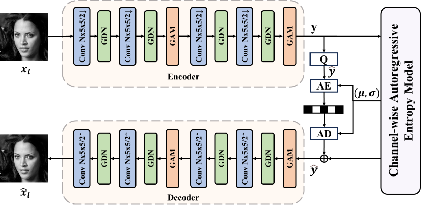
Architecture details. The structure for low frequency and residual compression is depicted in Fig.13. The encoder, denoted as E, maps the input image to a latent representation y. Following quantization by Q, we obtain the discrete representation of the latent variable, denoted as . This is subsequently transformed back to a reconstructed image through the decoder, represented as D. The core process is expressed as follows:
| (18) |
where and are trainable parameters of the encoder E and decoder D. We model each element as a single Gaussian distribution with its standard deviation and mean by introducing a side information . The distribution of is as follows:
| (19) |
To expedite the prediction process of the latent variable , we employ the Channel-wise Auto-regressive Entropy Model [25] for parallel accelerated prediction. This approach results in faster decoding.
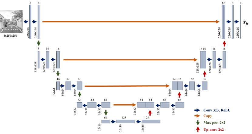
For our condition generation module, we design a deep U-net-like CNN architecture with a localized receptive field for estimating the score of probability of high frequency coefficients conditioned on low frequency coffcients. Specifically, the encoder’s downsampling module comprises two 3 x 3 convolutional layers and a 2 x 2 maximum pooling layer, each of which applied four times. The decoder’s upsampling module includes a deconvolutional layer and a feature splicing layer, repeated four times. The network implementation details are shown in Fig14.