RIS-Based Self-Interference Cancellation for Full-Duplex Broadband Transmission
Abstract
Full-duplex (FD) is an attractive technology that can significantly boost the throughput of wireless communications. However, it is limited by the severe self-interference (SI) from the transmitter to the local receiver. In this paper, we propose a new SI cancellation (SIC) scheme based on reconfigurable intelligent surface (RIS), where small RISs are deployed inside FD devices to enhance SIC capability and system capacity under frequency-selective fading channels. The novel scheme can not only address the challenges associated with SIC but also improve the overall performance. We first analyze the near-field behavior of the RIS and then formulate an optimization problem to maximize the SIC capability by controlling the reflection coefficients (RCs) of the RIS and allocating the transmit power of the device. The problem is solved with alternate optimization (AO) algorithm in three cases: ideal case, where both the amplitude and phase of each RIS unit cell can be controlled independently and continuously, continuous phases, where the phase of each RIS unit cell can be controlled independently, while the amplitude is fixed to one, and discrete phases, where the RC of each RIS unit cell can only take discrete values and these discrete values are equally spaced on the unit circle. For the ideal case, the closed-form solution to RC is derived with Karush-Kuhn-Tucker (KKT) conditions. Based on Riemannian conjugate gradient (RCG) algorithm, we optimize the RC for the case of continuous phases and then extend the solution to the case of discrete phases by the nearest point projection (NPP) method. Simulation results are given to validate the performance of our proposed SIC scheme.
Index Terms:
Reconfigurable intelligent surface (RIS), full-duplex (FD), self-interference cancellation (SIC), near-field, orthogonal frequency division multiplexing (OFDM).I Introduction
Full-duplex (FD) has gained substantial attention in recent years and is widely considered as an effective technology to enhance the spectrum efficiency. Compared with traditional half-duplex (HD), FD can potentially double the spectrum efficiency, thus inherently increasing the capacity of wireless networks. However, FD faces the problem of how to deal with the self-interference (SI) [1, 2, 3].
Reconfigurable intelligent surface (RIS) is an emerging material that consists of a large number of low-cost passive reflecting elements. Moreover, each unit cell of RIS can independently induce the amplitude and phase variations of the incident signal[4], thus cooperatively achieving fine 3D reflection beamforming. In the existing literature about RIS-assisted FD communications, the authors of [5] studied the beamforming optimization for a RIS-assisted FD communication system, where the SI is assumed to follow Gaussian distribution. Also, the authors of [6] studied the spatially correlated RIS-assisted multiuser FD massive multi-input-multi-output (mMIMO) system, where the SI is independent and identically distributed. Although RIS is combined with FD in [5] and [6], how to use RIS to deal with the strong SI was not discussed. The authors of [7] proposed a RIS-assisted FD wireless communication system that increases the effective path of the desired signal. However, the self-interference cancellation (SIC) capability is relatively small, because of the high power differential between the desired and interference signals. A RIS-assisted FD system is studied in [8], which analyzes the effects of residual SI, self-reflections and interference from the RIS. Simulation results of [8] suggest that RIS can counter the effect of the residual SI and can achieve the same outage probability as that in HD communications if the number of RIS meta-atoms is enough. This suggests the feasibility of utilizing RIS for SIC in FD communications.
On the other hand, with regard to RIS-assisted broadband transmission systems, the authors of [9] considered the capacity maximization for broadband transmission in a general MIMO orthogonal frequency division multiplexing (OFDM) system under frequency-selective fading channels. In [10], RISs are used in unmanned aerial vehicle (UAV)-based orthogonal frequency division multiple access (OFDMA) communication systems to enhance sum-rate. With a RIS, the composite channel from the UAV to ground users experiences both frequency-selectivity and spatial-selectivity fading. Besides, a RIS-assisted multi-carrier MIMO wireless physical layer security communication system was investigated in [11], which consists of a legitimate transmitter, a legitimate receiver, a RIS node, and an eavesdropper. It can be observed that while RIS-assisted FD transmission and RIS-assisted broadband transmission have been studied, how to deal with the SI for RIS-assisted FD broadband transmission is not well discussed.
To achieve miniaturization and portability of RIS-assisted FD devices, RISs are desired to be deployed inside the devices. Similar studies have been conducted in the area of visible light communication (VLC). In VLC, RIS can be deployed inside devices to enhance their performance. For example, [12] depicts an indoor VLC system where RIS assists in directing the received light and concentrating its beam on the photodetector (PD). It functions as a filter that permits light signals of specific wavelengths to pass while impeding unwanted light, resulting in reduced interference. The authors of [13] proposed and demonstrated that deploying liquid crystal (LC)-based RIS as part of the VLC receiver can improve data rate. The purpose of LC-RIS is providing incident light steering and intensity amplification to improve the received signal strength and the corresponding achievable data rate. The indoor VLC system is composed of a VLC-enabled ceiling light emitting diode array and a user equipped with a nematic LC RIS-based VLC receiver. The feasibility of miniaturized RISs with similar size to the RIS in this paper has also been demonstrated in existing works. For examples, the authors of [14] proposed and demonstrated the use of a 6-by-8 unit metasurface to protect sensitive devices from large signals, while still allowing a communication channel for small signals. The authors of [15] fabricated a novel ultrathin linear-to-cross-polarization transmission converter based on a metasurface (having unit cells).
Inspired by the above works related to VLC where RISs can be deployed inside devices to enhance performance, in this paper we consider an FD broadband wireless communication system where small RISs are deployed inside FD devices to cancel SI. With the proposed design for the reflection coefficient (RC) matrix of the RIS, the SI can be significantly canceled, which promises the double data rate as compared with HD. The main contributions of this paper are summarized as follows:
-
1)
To the best of our knowledge, this is the first work to study RIS-assisted FD-OFDM communication system where small RISs are deployed inside FD devices to mitigate the strong SI by passive beamforming. The system consists of two FD devices and each device is equipped with a single transmit antenna, a single receive antenna, and a RIS. The RIS-based SIC scheme developed in this paper is a new attempt of SIC in the propagation domain. Furthermore, the deployment of small RISs within communication terminals showcases a new application scenario for RIS-assisted wireless communications.
-
2)
Since small RISs are deployed inside devices, it is essential to account for the near-field behavior of the RIS. RIS-assisted FD-OFDM system is accurately modeled by the near-field channel model, which ensures its effectiveness for broadband transmission in this scenario.
-
3)
To enhance the performance of the new SIC scheme for broadband transmission, we formulate an optimization problem to maximize the SIC capability. Given the non-convexity of the optimization problem, an alternate optimization (AO) algorithm is developed to jointly optimize the power allocation vector and RC matrix in three cases. Specifically, for the fixed RC, the closed-form solution to power allocation is derived. For the fixed power allocation vector, quadratic transform, Karush-Kuhn-Tucker (KKT) conditions, Riemannian conjugate gradient (RCG) algorithm, and nearest point projection (NPP) method are adopted to optimize the RC matrix.
-
4)
Finally, numerical results are presented to validate the performance of the proposed SIC scheme and the effectiveness of the RIS phase shift design. Numerical results demonstrate that the capacity gain of RIS-assisted FD-OFDM system over HD-OFDM system without RISs can be more than 2.25 times.
The rest of the paper is organized as follows. Section II gives the system model for the proposed RIS-based SIC scheme and analyzes the near-field behavior of the RIS. In Section III, an optimization problem is formulated to maximize the SIC capability. Then we utilize AO algorithm to jointly optimize the power allocation vector and RC matrix in three cases, with the goal of minimizing residual SI. Simulation results are given in Section IV to verify the performance of the proposed SIC scheme. This paper concludes with Section V.
Notations: Boldface straight lowercase and uppercase letters denote vectors and matrices, respectively. denotes the space of complex matrices, denotes the space of real matrices, and denotes the maximum between two real numbers and . For a matrix of arbitrary size, , , and denote the conjugate transposed matrix, the Frobenius norm, and the conjugate of , respectively. Further, we use and to denote an identity matrix and all-zero matrix of appropriate dimensions, respectively. and stands for “defined as” and “distributed as”, respectively. denotes the modulo operation, denotes round down, and denotes Hadamard product. The distribution of a circularly symmetric complex Gaussian (CSCG) random variable with mean and variance is denoted by . indicates a complex random vector following the distribution of mean and covariance matrix . denotes the absolute value operation, denotes the operation of trace, denotes the arctangent function, and denotes a square diagonal matrix with the elements of on the main diagonal. and denote the angle and the real part of a complex number, respectively.
| (3) |
II System Model
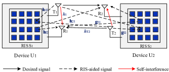
As shown in Fig. 1, we consider an FD-OFDM communication system where two FD devices (denoted by and ) exchange information with each other under frequency-selective fading channels. Both FD devices have a single transmit and receive antenna. We assume that each device is equipped with a RIS which contains reflection elements to assist FD wireless communications. The RIS assists the FD device through its reflection elements which could control the amplitude and phase of the incident signal independently. The receive antenna receives not only the SI signal but also the reflected signal, which is utilized to diminish the SI signal. Thus, the SI can be significantly canceled.
The reconfigurability of RIS lies not only in the amplitude and phase, but also in frequency and polarization shifts [16]. In this paper, the RIS is deployed inside the device, and the positions of the transmit antenna, the receive antenna, and the RIS are fixed. While the RIS channel gain is not affected by the distance between the antennas and the RIS, this paper considers a wideband OFDM system where the RIS channel gain is also affected by the frequency. The RIS channel varies with the frequency, and if the bandwidth exceeds the available bandwidth, it is necessary to reconfigure the wireless environment to ensure the performance gain of the RIS, which reflects the reconfigurability of RIS [17].
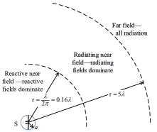
We consider the case where the operating frequency is GHz[18] and the wavelength is m. Also, RISs are considered small and deployed inside FD devices. The distance between the transmitter/receiver of each FD device and each unit cell of its equipped RIS is assumed to be larger than and less than . According to the definition of the near-field and far-field [19] for the small-size antenna shown in Fig. 2, the transmitter/receiver of each FD device is in the radiating near-field of each unit cell of its equipped RIS. The near-field behavior and far-field behavior of the RIS are different. There are three differences between the near-field and the far-field [20]: the distance to each unit cell, the effective unit cell areas, and the loss from polarization mismatch. Considering the above three differences, in the following the near-field behavior of the RIS is analyzed and utilized to mitigate SI.
II-A Channel Model
Based on previous RIS-assisted FD-OFDM system model, the channel model is introduced in this subsection. We define the number of OFDM subcarriers as and the indexes of subcarriers are denoted by . Thus the subcarrier spacing , where denotes the transmission bandwidth. We let and denote the SI channel gains of device and device on the th subcarrier, respectively. The frequency-domain channel from transmit antenna to receive antenna , from RIS to receive antenna , and from transmit antenna to RIS on the th subcarrier are denoted by , , and , respectively. The frequency-domain channel from transmit antenna to receive antenna , from RIS to receive antenna , and from transmit antenna to RIS on the th subcarrier are denoted by , , and , respectively. The frequency-domain channel between transmit antenna and RIS on the th subcarrier is denoted by and that between receive antenna and RIS on the th subcarrier is denoted by . Similarly, the frequency-domain channel between transmit antenna and RIS on the th subcarrier is denoted by and that between receive antenna and RIS on the th subcarrier is denoted by . In this paper, we assume that both RISs only reflect once since the power of the signal reflected two or more times is much smaller than that of the signal reflected once [21], [22]. Moreover, the channel gains of -- link and -- link can be neglected due to the long distance [5], [6]. In this paper, we assume that wireless channels experience quasi-static block-fading and the channel state information (CSI) is known to FD [6, 23].
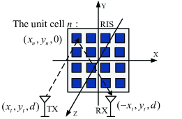
We set up a right-angle coordinate system for each FD device to compute the coordinate of the center of each unit cell and analyze the near-field channel of RIS. As shown in Fig. 3, the center of RIS is located at the coordinate origin of the XY-plane. Also, both the transmit antenna and the receive antenna are located in the XZ-plane and they are symmetric about the Z axis. The coordinates of the transmit and receive antenna are denoted by and , respectively. We consider the RIS is square where the cells are deployed edge-to-edge and each RIS unit cell has an area of on the th subcarrier. If we number the unit cells from left to right, row by row, the coordinate of the center of the th unit cell on the th subcarrier is with
| (1) |
and
| (2) |
We denote by the near-field channel on the th subcarrier where and use an exact model, which takes into account the near-field behavior of the RIS, to quantify it [24], [25]. We consider that the transmit antenna located at is lossless isotropic and transmits a signal that has polarization in the Y direction when traveling in the Z direction. The channel amplitude gain on the th subcarrier at the th unit cell , located at , can be given by (3) at bottom of this page, where
| (4) |
and
| (5) |
Based on (3), (4), and (5), the channel gain on the th subcarrier between the transmit antenna and the RIS can be given by
| (6) |
where and with
| (7) |
and
| (8) |
In (8), is the wavelength of the -th subcarrier with the frequency of
| (9) |
Similarly, we can also obtain the channel gain on the th subcarrier between the RIS and the receive antenna using the above model. Since the transmit and receive antenna coordinates are fixed, the modulus of the SI channel gain remains constant under different subcarriers. However, the phase of the SI channel gain varies under different subcarriers. The expression for the near-field channel gain of RIS provided in this paper is derived by treating each RIS unit cell as a receive antenna [24, 25]. Thus, when calculating the SI gain between the transmit and receive antenna, we can consider the receive antenna as a RIS which has only one unit cell. Following similar steps, the SI channel gain on the th subcarrier between the transmit antenna and the receive antenna of each FD device can be expressed as follows:
| (10) |
where . The coefficients and in (10) can be equivalently calculated based on (3), (4), (5) and (8) with and . Note that the employed channel model is applicable to the radiating near-field, but not to the reactive near-field [24, 25]. We assume that the transmitter/receiver of each FD device is in the radiating near-field of each unit cell of its equipped RIS, such that the channel model is accurate.
The far-field channel on the th subcarrier is denoted by , then we model it with Rician fading. For a Rician channel with K-factor denoted by , the channel matrix can be given as follows:
| (11) |
where denotes a large number of secondary non-light of sight (NLOS) channel gains, denotes the normalized complex light of sight (LOS) channel gains between the transceiver antennas, and denotes the corresponding pathloss. We can obtain the far-field channel on the th subcarrier from the following equation
| (12) |
where denotes the th column of the discrete Fourier transform (DFT) matrix .
II-B Signal Model
Without loss of generality, in the following we only analyze the transmission from to with the assistance of and . The presented analyses and scheme can be extended for the transmission from to with the assistance of and in a straightforward manner. We denote by and the OFDM symbol transmitted from transmit antenna and that from transmit antenna , respectively, where and are the OFDM symbols on the th subcarrier. These OFDM symbols are first transformed into the time domain via an -point inverse discrete Fourier transform (IDFT), and then appended by a cyclic prefix (CP) of length . We assume that the length of CP is longer than the maximum delay spread of all channels, denoted by , to eliminate the inter-symbol interference (ISI). Moreover, let and where , denote the power allocated to the th subcarrier of and , respectively. Assume the transmit power constraint at is and the transmit power constraint at is . Thus the power allocation at and should satisfy and , respectively. In fact, when we design phase shift control circuits, RIS can only bring the same phase shift on different subcarriers. Thus we model the RC matrix of RIS as , where is the reflection efficiency and with is the RC of the th unit cell of RIS . In the same way, we model the RC matrix of RIS as , where is the reflection efficiency and with is the RC of the th unit cell of RIS . Considering the practical implementation of the RIS, we assume that the feasible set of RC has the following three cases:
- 1)
- 2)
- 3)
By analyzing the three cases of the RIS, we can comprehensively understand the characteristics and performances of RIS-assisted FD-OFDM communication system [22]. The continuous and discrete phases case have lower manufacturing complexity compared to the ideal phases case which requires simultaneous adjustment of both phase and amplitude. This can ultimately provide a better guidance and support for practical applications.
After removing CP and performing -point DFT, the received signal on the th subcarrier at the receiver of device is expressed as follows:
| (16) |
where is the additive white Gaussian noise (AWGN) on the th subcarrier.
After simplification, (16) can be re-written as follows:
| (17) |
where with , with , and with . Moreover, and denote the RC vector of RIS and RIS , respectively. We define and the received OFDM symbol at the receiver of device can be re-written as follows:
| (18) |
where is the channel frequency response (CFR) of - link, is the CFR of SI channel, with is the equivalent cascaded CFR of -- link, with is the equivalent cascaded CFR of -- link, and with is the equivalent cascaded CFR of -- link. and denote the diagonal matrix of OFDM symbol and OFDM symbol , respectively. Moreover, denotes the AWGN vector at , which follows . In addition, represents the desired signal, is the SI, and is the RIS-assisted signal to cancel the severe SI. The SIC performance can be measured by the SIC capability (dB) [30], which is defined as follows:
| (19) |
where is the energy of the SI signal before SIC, is the energy of the residual SI after SIC, and is the energy of noise.
Substituting Eq. (17) into Eq. (19), we have the SIC capability of RIS-assisted FD-OFDM communications as follows:
| (20) |
Furthermore, the system capacity after SIC can be expressed as follows:
| (21) |
Given the same bandwidth, the capacity of HD-OFDM communication system without RIS-based SIC can be given by
| (22) |
III SIC Capability Maximization Via Joint Power Allocation And Reflection Coefficient Optimization
In this section, the RC matrix of the RIS and power allocation scheme of each device are jointly optimized to maximize the SIC capability shown in (20). We first formulate the optimization problem and then propose an AO algorithm to solve it.
III-A Problem Formulation
Considering the constraints of the transmit power and the RC, the SIC capability maximization problem is formulated as follows:
| (23a) | ||||
| s.t.: | (23b) | |||
| (23c) | ||||
| (23d) | ||||
where is chosen from , , and . If or , constraint (23d) is non-convex. Moreover, the objective function of (P1) is non-convex. Thus, (P1) is a non-convex problem and is difficult to solve directly. To overcome the above challenges, in the following we propose an AO algorithm which optimizes and iteratively to find an approximate solution to (P1).
III-B Power Allocation Optimization with Given Reflection Coefficient
In this subsection, we optimize power allocation vector for the given RC vector. Due to the fixed RC vector, the superimposed CFR is fixed, then problem (P1) can be transformed into
| (24a) | ||||
| s.t.: | (24b) | |||
| (24c) | ||||
where , , and constraint (23d) is omitted because is fixed. Note that (P2) is a multiple-ratio fractional programming (FP) problem which is difficult to solve, thus we use the quadratic transform [31] to transform (P2) into the following problem
| (25a) | ||||
| s.t.: | (25b) | |||
| (25c) | ||||
| (25d) | ||||
where includes the introduced auxiliary variables . When the power allocation vector is fixed, the closed-form solution to can be derived as follows:
| (26) |
When is fixed, (P3) can be simplified to
| (27a) | ||||
| s.t.: | (27b) | |||
| (27c) | ||||
Notice that is concave with respect to , thus (P3′) is a convex problem which can be solved with KKT conditions[32]. We can write the Lagrangian function corresponding to (P3′) as follows:
| (28) |
where
| (29) |
with is the Lagrange multiplier vector, and is the Lagrange multiplier. According to KKT conditions, we have
| (30) |
Solving (30), the closed-form solution to (P3′) can be directly derived as follows:
| (31) |
where
| (32) |
should be chosen to satisfy . The optimal solution to and can be found by sub-gradient method or ellipsoid method [32].
III-C Reflection Coefficient Optimization with Given Power Allocation
For the given multi-carrier power allocation, the optimization of the RC in three cases is discussed in this subsection. We only show the optimization steps for RC vector . RC vector can be optimized in the same manner. Due to the fixed power allocation vector , (P1) can be simplified as follows:
| (33a) | ||||
| s.t.: | (33b) | |||
where constraints (23b) and (23c) are omitted because of the fixed power allocation vector . Notice that, similar to the previous subsection, (P4) is a multiple-ratio FP problem. Similarly, we introduce , which includes the introduced auxiliary variables and then use the quadratic transform to transform (P4) into the following problem
| (34a) | ||||
| s.t.: | (34b) | |||
| (34c) | ||||
where
| (35) |
When is fixed, the closed-form solution to can be found as follows:
| (36) |
Because of the fixed and , maximizing is equivalent to minimizing . We first omit irrelevant items and then transform (P5) into
| (37a) | ||||
| s.t.: | (37b) | |||
where
| (38) |
with
| (39) |
| (40) |
and
| (41) |
Notice that (III-C) is a quadratic convex function with respect to . Thus, (P6) is a quadratically constrained quadratic programming (QCQP). If , (P6) is a convex QCQP and its closed-form solution can be directly obtained using convex optimization tools. If or , (P6) is a non-convex problem and we can only obtain a suboptimal solution to (P6).
1) If , constraint (37b) is
| (42) |
which can be re-written as follows:
| (43) |
where is a column vector whose elements are all zero except that the th is one. Thus, (P6) can be further transformed into
| (44) | ||||
| s.t. |
Note that (P6′) is convex and can be solved with KKT conditions. We can write the Lagrangian function corresponding to (P6′) as follows:
| (45) |
where is the Lagrange multiplier vector with for . According to KKT conditions, we have
| (46) |
Solving (46), we can obtain the optimal solution as follows:
| (47) |
where the optimal , denoted by , can be obtained by sub-gradient method or ellipsoid method.
2) If , constraint (37b) is
| (48) |
which is equivalent to Then, (P6) can be transformed into the following problem
| (49a) | ||||
| s.t. | (49b) | |||
Due to the non-convex constraint (49b), (P6′′) is a non-convex QCQP. In general, the unit modulus constraint problem is solved by dropping the rank-one constraint using semidefinite relaxation (SDR) method [27]. However, SDR method has high computational complexity and may not converge to a good suboptimal solution. Thus, we propose RCG algorithm to solve (P6′′).
According to [33, 34], unit modulus constraint (49b) forms an -dimensional complex circle manifold denoted as follows:
| (50) |
where complex circle manifold is a Riemannian sub-manifold of Riemannian manifold . Thus, (P6′′) can be formulated as the following problem
| (51) |
where (P7) is an unconstrained problem on the surface of . For any point on , the tangent space formed by passing through this point can be represented as
| (52) |
where is a tangent vector passing through .
Riemannian gradient [34] is defined as the tangent vector or direction in the Riemannian tangent space, which represents the direction of the fastest change of the objective function. Since is a Riemannian sub-manifold, the Riemannian gradient of at point , denoted by , can be expressed as follows:
| (53) |
where denotes the orthogonal projection of the Euclidean gradient onto . Through numerical computation, we can obtain the Euclidean gradient at point as follows:
| (54) |
Since the tangent vector obtained from the Riemannian gradient may not lie on the surface of the manifold, we need a retraction operation to map this vector to a new point on the manifold. This map procedure can be expressed as follows:
| (55) |
where denotes the search direction passing through , is the Armijo backtracking line search step size, denotes the operation of mapping, and denotes the normalization of vector.
With conjugate gradient descent method, the th search direction in Euclidean space is
| (56) |
where is the Polak-Ribiere parameter of the th iteration [34]. Since and lie on different tangent spaces and cannot be conducted directly with mathematical computation, at point needs to be transported to at point , the transport operation is given by
| (57) |
With the Riemannian gradient, the th search direction in the manifold space can be updated by
| (58) |
The specific procedure of RCG algorithm to solve (P6′′) is summarized in Algorithm 1, which continuously updates the gradient search direction based on (58) until the Riemannian gradient converges. The complexity of RCG algorithm is mainly dominated by calculating the Euclidean gradient, which is . Thus, the computational complexity of RCG algorithm is where represents the iteration times required by the RCG algorithm. According to [32], the complexity of SDR method is . It can be observed that the complexity of RCG algorithm is lower than that of the SDR method.
3) If , the constraint of (P1) is
| (59) |
We adopt NPP method to deal with the discrete phase and choose to obtain the discrete phase RC from the projection of the continuous phase RC due to the relatively low computational complexity [22]. We denote by the angle of the optimal solution to (P6′′). Then, for the case where , we can obtain the subptimal solution to the discrete phase as follows:
| (60) |
where
| (61) |
III-D Overall Algorithm
Based on previous discussions, the AO algorithm to solve (P1) is shown in Algorithm 2. The specific steps of the algorithm are as follows: Firstly, the algorithm starts with initial feasible points and . In the next step, with a fixed solution and from the th iteration, the update of and is performed alternately using fractional programming techniques in the th iteration. Note that the objective function of (P1) is monotonically non-decreasing, hence Algorithm 2 will eventually converge[11].
IV Simulation
In this section, we give simulation results under different conditions to validate the SIC capability and the capacity gain of RIS-assisted FD-OFDM communications over HD-OFDM communications.
We assume that the transmit and receive antenna of each FD device is located at m and m, respectively. The number of OFDM subcarriers, the maximum delay spread, and the length of CP is set to , , and , respectively. We set the distance between two FD devices to 1000 m, the area of each unit cell under the th subcarrrier to , and the reflection efficiency of each RIS to . Also, the total power of each transmitter is set to , the noise power is set to dBm, and . The pathloss is given by , where is the distance and is the pathloss at the reference distance of 1 m, which is set to -30 dB with the pathloss exponent of . If , we set . If , we set . The channels between elements of a RIS and an antenna are assumed to be independent and identically distributed. However, the channels from a RIS to different antennas are assumed to be non-identical. Apart from our schemes developed in Section III, we also introduce benchmark scheme for comparison. The descriptions of our developed and the benchmark scheme are as follows:
-
1)
Ideal case: in this scheme, both the RC matrix of the RIS and power allocation vector are optimized to maximize the SIC capability under the case of .
-
2)
Continuous phases: we apply RCG algorithm to optimize the RC matrix where .
-
3)
Discrete phases: when the phase shift belongs to the set , we set the number of discrete phases to be and for comparison.
-
4)
Random phases: we set the random phases scheme as the benchmark scheme. In our assumption, the RC has a random phase that is randomly selected from [0, ], while the amplitude is fixed to one [35].
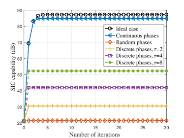
First, we evaluate the convergence behavior of Algorithm 2. The number of RIS elements is set as , the transmit power is set as dBm, and the signal bandwidth is set as MHz. If not mentioned otherwise, these parameter settings remain constant throughout the subsequent discussion. We initialize the power allocation vector as a column vector of zeros and the RC vector as a column vector of ones, except for the random phases scheme where the phase of each unit cell is initialized as a random value selected from [0, ]. Fig. 4 shows the SIC capability versus the number of iterations in different conditions. We can observe from Fig. 4 that all curves converge within 5 iterations. To be specific, the ideal case and the continuous phases case converge within 5 iterations, while the other cases converge within 1 iteration. For the ideal phases case, the power allocation vector and RC vector are obtained by solving the KKT conditions, which can be expressed in closed-form expression. Thus, the optimal solution can be obtained in each iteration, resulting in convergence. In addition, the RC vector of the continuous phases case is optimized by the RCG algorithm, which also offers a fast convergence. Thus, the continuous phases curve can converge within 5 iterations. The discrete phases case converges faster than the ideal and continuous phases cases for two reasons. First, the feasible domain of the discrete phases case is small, we only need to choose one of several discrete values as the phase shift. Second, the discrete phases are directly projected from the continuous phases. Thus, we only need to optimize the power allocation without optimizing the RC. Similarly, the random phases are generated randomly, and only the power allocation is optimized, resulting in the same fast convergence speed as the discrete phases. Since both the amplitude and phase of each RIS unit cell can be independently and continuously controlled, the ideal case can achieve the optimal performance, which is consistent with the discussion in Section II.
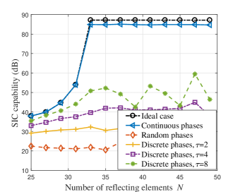
In Fig. 5, the SIC capability and capacity gain are depicted with different values of . As shown in Fig. 5(a), the SIC capabilities of the ideal case and the continuous phases case increase monotonically as the value of increases and it can be larger than 85 dB. When is larger than 32, both the ideal case and the continuous phases case exhibit a consistent SIC capability that remains stable as increases. The curve of the ideal case can remain stable because the modules of the RC are not fixed to one. This stability of the continuous phases case is achieved because the optimized power allocation vector compensates for the unit modulus constraint and ensures that the SIC capability does not decrease as increases. Increasing the value of leads to an enhancement in the SIC capability of the discrete phases because the candidate phases approach the ideal phases more closely as increases. However, as compared with the cases of ideal phases and continuous phases, the SIC capability of the discrete phases is weaker due to the phase differences between candidate phases and ideal phases. In the case of discrete phases, the SIC capability fluctuates with the increase of due to the varying phase differences. At times, these phase differences increase, leading to a decrease in SIC capability. Conversely, there are instances where the phase differences decrease, resulting in an increase in SIC capability. Thus, the fluctuation of SIC capability with can be attributed to the changing phase differences. This reduction in SIC capability resulting from these phase differences can be compensated by increasing the number of reflecting elements. The SIC achieved with random phases is approximately 20 dB, which is significantly lower than that of the ideal case and the continuous phases case. This result implies the importance of phase shift design in SIC.
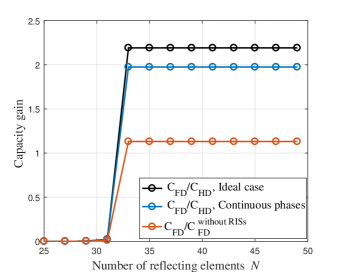
The comparison of our proposed RIS-assisted FD-OFDM system with the FD-OFDM system without RISs is shown in Fig. 5(b). The system capacity of FD-OFDM system without RISs are obtained by replacing (21) with
| (62) |
where is the SIC coefficient [36, 37, 38]. When , the SI is perfectly canceled. On the other hand, when , SIC techniques are invalid. To better clarify the capacity gain of the proposed RIS-assisted FD-OFDM communication system over FD-OFDM system without RISs, we set where 87 dB is the SIC capability of RIS-assisted FD-OFDM system. As illustrated in Fig. 5(b), the capacity gain is initially close to zero due to the strong SI. However, the capacity gain gradually increases as increases, and then ultimately reaches a steady state. It is worth noting that although RISs are deployed to cancel the SI, the RIS-assisted link indirectly strengthens the desired signal. Thus, the capacity gain of the proposed RIS-assisted FD-OFDM communication system over HD-OFDM system without RISs can be more than 2.25 times. With the same SIC capability, we can observe that the capacity gain of RIS-assisted FD-OFDM communication system over FD-OFDM system without RISs is 1.13, which confirms that RIS can significantly improve the capacity as compared with FD-OFDM communication system without RISs. This is because the RIS-assisted link not only cancels the SI but also strengthens the desired signal. The results in Fig. 5 demonstrate the feasibility of deploying RIS for SIC and provide a novel approach for SIC in the propagation domain for FD communications.
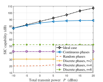
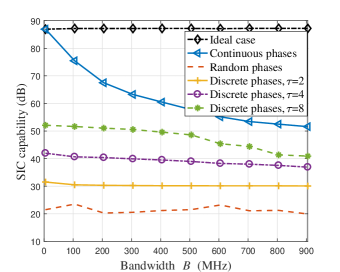
Figure 6 plots the SIC capability corresponding to the total transmit power . Fig. 6 illustrates that as increases, the SIC capabilities of the ideal case and the continuous phases case increase accordingly. However, the SIC capability of the continuous phases case is weaker than that of the ideal case due to the unit modulus constraint imposed on each RIS units, which limits its performance. In cases of discrete phases and random phases, the SIC capabilities are not affected by transmit power. Hence, increasing fails to improve the SIC capability. This outcome is attributed to the inadequate cancellation of SI. The residual SI remains very strong, which diminishes the significance of transmit power in increasing the SIC capability.
In Fig. 7, the SIC capability of the proposed scheme with different values of signal bandwidth is presented. Fig. 7 shows that the SIC capabilities of all curves, except for the ideal case and the random phases case, decreases as increases. The reason for the curve of the ideal case remains unchanged is that the SI is effectively canceled, so it is not affected by bandwidth. The reason why the case of random phases is not affected by bandwidth, as same as Fig. 6, is the strong residual SI. The performance of the continuous phases case is similar to the ideal case when MHz, and then the SIC capability drops to dB when MHz due to the unit-modulus constraint. In practical design of RIS phase shift, passive beamforming with phase gradient metasurfaces can be used to cancel SI. The phase difference between different frequency points in the feasible signal bandwidth range is relatively constant, which implies that signal bandwidth has no impact on the SIC capability. The aforementioned development is encouraging, as it suggests that the implementation of RISs to cancel SI in FD broadband communications is feasible.
We can utilize phase discretization to simulate the phase errors of continuous phases. As the number of discrete phases increases, the phase errors decrease. When the number of phases approaches infinity, the phase errors become zero. The phase errors are defined by
| (63) |
where denotes the ideal phase of the continuous phases case and is the actual phase of the th unit cell selected from the available phases.
Figure 8 presents the SIC capability corresponding to different numbers of discrete phases . We set to increase by , where is the resolution bits for the discrete phases.

As shown in Fig. 8, the SIC capability gradually increases as increases. When , the SIC capability of the discrete phases is close to that of the continuous phases, with phase errors of about . When , i.e., the phase error is , which is larger than the actual engineering design error [39, 40]. However, the SIC capability only decreases by 5 dB, and there is still 80 dB of SIC capability, which is enough to ensure the performance of the RIS. Thus, the phase accuracy of the proposed RIS-assisted FD-OFDM communication system is sufficient.
The size of RIS is the primary limiting factor for deploying it inside a device. For the considered 5.8 GHz band, RIS can be deployed inside a device since its size can be relatively small. The RIS unit side length can typically be selected between and [4, 24]. We can set the RIS unit length to . For the case where the operating frequency is GHz, the wavelength is m, and the area of RIS unit cell is . As shown in Fig. 5(a) of this paper, a total of 36 RIS units are required to achieve maximum SIC capability. Therefore, the size of RIS is approximately , which can be deployed inside some terminal products, such as HUAWEI CPE series.
V Conclusions
In this paper, we proposed and analyzed a novel SIC scheme based on RIS for FD-OFDM communications. First, we analyzed the near-field behavior of the RIS and found the relationships between near-field channel and performance optimization. We then formulated an optimization problem to maximize the SIC capability by controlling the RC of the RIS and allocating the transmit power of the device. Finally, we utilized the AO algorithm to solve the problem in ideal case, continuous phases, and discrete phases. Simulation results showed that the proposed RIS-based SIC scheme can cancel the SI by more than 85 dB in the ideal case and the continuous phases case. Furthermore, we evaluated the impact of phase errors caused by small-sized RIS in SIC capability. The unsignificant difference in SIC capability between two cases indicates that the low-complexity RIS with fixed amplitude of 1 is a viable option. Also, the capacity gain of the proposed RIS-assisted FD-OFDM system over HD-OFDM system without RISs can be more than 2.25 times due to the enhancement for the effective path of the desired signal. These encouraging results suggest that RIS can provide an attractive way to achieve FD communications.
References
- [1] W. Cheng, W. Zhang, L. Liang, and H. Zhang, “Full-duplex for multi-channel cognitive radio ad hoc networks,” IEEE Network, vol. 33, no. 2, pp. 118–124, 2019.
- [2] S. A. Jiménez, J. S. Garcia, and F. R. C. Soria, “Self interference cancellation on a full duplex DFTs-OFDM system using GNU radio and USRP,” IEEE Latin America Transactions, vol. 19, no. 10, pp. 1781–1789, 2021.
- [3] S. M. Kim, Y. G. Lim, L. Dai, and C. B. Chae, “Performance analysis of self-interference cancellation in full-duplex massive MIMO systems: subtraction versus spatial suppression,” arXiv preprint arXiv:2205.14475, 2022.
- [4] W. Tang, M. Z. Chen, X. Chen, J. Y. Dai, Y. Han, M. D. Renzo, Y. Zeng, S. Jin, Q. Cheng, and T. J. Cui, “Wireless communications with reconfigurable intelligent surface: path loss modeling and experimental measurement,” IEEE Transactions on Wireless Communications, vol. 20, no. 1, pp. 421–439, 2021.
- [5] H. Shen, T. Ding, W. Xu, and C. Zhao, “Beamformig design with fast convergence for IRS-aided full-duplex communication,” IEEE Communications Letters, vol. 24, no. 12, pp. 2849–2853, 2020.
- [6] N. V. Deshpande, S. Dey, D. N. Amudala, and R. Budhiraja, “Spatially-correlated IRS-aided multiuser FD mMIMO systems: analysis and optimization,” IEEE Transactions on Communications, vol. 70, no. 6, pp. 3879–3896, 2022.
- [7] P. K. Sharma and P. Garg, “Intelligent reflecting surfaces to achieve the full-duplex wireless communication,” IEEE Communications Letters, vol. 25, no. 2, pp. 622–626, 2020.
- [8] S. Dhok and P. K. Sharma, “Infinite and Finite Block-length FD Transmissions with Spatially-correlated RIS Channels,” IEEE Transactions on Wireless Communications, 2022.
- [9] S. Zhang and R. Zhang, “Capacity characterization for intelligent reflecting surface aided MIMO communication,” IEEE Journal on Selected Areas in Communications, vol. 38, no. 8, pp. 1823–1838, 2020.
- [10] Z. Wei, Y. Cai, Z. Sun, D. W. K. Ng, J. Yuan, M. Zhou, and L. Sun, “Sum-rate maximization for IRS-assisted UAV OFDMA communication systems,” IEEE Transactions on Wireless Communications, vol. 20, no. 4, pp. 2530–2550, 2021.
- [11] W. Jiang, B. Chen, J. Zhao, Z. Xiong, and Z. Ding, “Joint active and passive beamforming design for the IRS-assisted MIMOME-OFDM secure communications,” IEEE Transactions on Vehicular Technology, vol. 70, no. 10, pp. 10 369–10 381, 2021.
- [12] S. Aboagye, A. R. Ndjiongue, T. M. Ngatched, O. A. Dobre, and H. V. Poor, “RIS-assisted visible light communication systems: A tutorial,” IEEE Communications Surveys & Tutorials, 2022.
- [13] S. Aboagye, A. R. Ndjiongue, T. M. Ngatched, and O. A. Dobre, “Design and Optimization of Liquid Crystal RIS-Based Visible Light Communication Receivers,” IEEE Photonics Journal, vol. 14, no. 6, pp. 1–7, 2022.
- [14] X. Yang, E. Wen, and D. F. Sievenpiper, “Power-dependent metasurface with self-induced bandgap,” IEEE Antennas and Wireless Propagation Letters, vol. 21, no. 6, pp. 1115–1119, 2022.
- [15] A. K. Baghel, S. S. Kulkarni, and S. K. Nayak, “Linear-to-cross-polarization transmission converter using ultrathin and smaller periodicity metasurface,” IEEE Antennas and Wireless Propagation Letters, vol. 18, no. 7, pp. 1433–1437, 2019.
- [16] M. M. Amri, “Recent Trends in the Reconfigurable Intelligent Surfaces (RIS): Active RIS to Brain-controlled RIS,” in 2022 IEEE International Conference on Communication, Networks and Satellite (COMNETSAT), 2022, pp. 299–304.
- [17] L. Zhang, X. Q. Chen, S. Liu, Q. Zhang, J. Zhao, J. Y. Dai, G. D. Bai, X. Wan, Q. Cheng, G. Castaldi et al., “Space-time-coding digital metasurfaces,” Nature communications, vol. 9, no. 1, p. 4334, 2018.
- [18] R. B. Green, K. Ding, V. Avrutin, U. Ozgur, and E. Topsakal, “Optically transparent antenna arrays for the next generation of mobile networAks,” IEEE Open Journal of Antennas and Propagation, vol. 3, pp. 538–548, 2022.
- [19] W. L. Stutzman and G. A. Thiele, Antenna theory and design. John Wiley & Sons, 2012.
- [20] A. D. J. Torres, L. Sanguinetti, and E. Björnson, “Near-and far-field communications with large intelligent surfaces,” in 2020 54th Asilomar Conference on Signals, Systems, and Computers, 2020, pp. 564–568.
- [21] L. You, J. Xiong, D. W. K. Ng, C. Yuen, W. Wang, and X. Gao, “Energy efficiency and spectral efficiency tradeoff in RIS-aided multiuser MIMO uplink transmission,” IEEE Transactions on Signal Processing, vol. 69, pp. 1407–1421, 2021.
- [22] H. Guo, Y. C. Liang, J. Chen, and E. G. Larsson, “Weighted sum-rate optimization for intelligent reflecting surface enhanced wireless networks,” arXiv preprint arXiv:1905.07920, 2019.
- [23] M. Hua and Q. Wu, “Joint dynamic passive beamforming and resource allocation for IRS-aided full-duplex WPCN,” IEEE Transactions on Wireless Communications, 2022.
- [24] E. Björnson and L. Sanguinetti, “Power scaling laws and near-field behaviors of massive MIMO and intelligent reflecting surfaces,” IEEE Open Journal of the Communications Society, vol. 1, pp. 1306–1324, 2020.
- [25] D. Dardari, “Communicating with large intelligent surfaces: fundamental limits and models,” IEEE Journal on Selected Areas in Communications, vol. 38, no. 11, pp. 2526–2537, 2020.
- [26] W. Tang, J. Y. Dai, M. Z. Chen, K. K. Wong, X. Li, X. Zhao, S. Jin, Q. Cheng, and T. J. Cui, “MIMO transmission through reconfigurable intelligent surface: System design, analysis, and implementation,” IEEE Journal on Selected Areas in Communications, vol. 38, no. 11, pp. 2683–2699, 2020.
- [27] Q. Wu and R. Zhang, “Intelligent reflecting surface enhanced wireless network: joint active and passive beamforming design,” in 2018 IEEE Global Communications Conference (GLOBECOM), 2018, pp. 1–6.
- [28] J. An, C. Xu, L. Gan, and L. Hanzo, “Low-complexity channel estimation and passive beamforming for RIS-assisted MIMO systems relying on discrete phase shifts,” IEEE Transactions on Communications, vol. 70, no. 2, pp. 1245–1260, 2022.
- [29] Z. Sun and Y. Jing, “On the performance of multi-antenna IRS-assisted NOMA networks with continuous and discrete IRS phase shifting,” IEEE Transactions on Wireless Communications, vol. 21, no. 5, pp. 3012–3023, 2022.
- [30] W. Cheng, J. Wang, R. Zhang, and H. Zhang, “Achieving maximum spectrum efficiency for full-duplex MIMO: the fractal array-element based self-interference mitigation approach,” IEEE Access, vol. 7, pp. 74 056–74 069, 2019.
- [31] K. Shen and W. Yu, “Fractional programming for communication systems—part i: Power control and beamforming,” IEEE Transactions on Signal Processing, vol. 66, no. 10, pp. 2616–2630, 2018.
- [32] S. Boyd, S. P. Boyd, and L. Vandenberghe, Convex optimization. Cambridge university press, 2004.
- [33] R. Li, B. Guo, M. Tao, Y.-F. Liu, and W. Yu, “Joint design of hybrid beamforming and reflection coefficients in RIS-aided mmWave MIMO systems,” IEEE Transactions on Communications, vol. 70, no. 4, pp. 2404–2416, 2022.
- [34] P. Absil, R. Mahony, and R. Sepulchre, Optimization algorithms on matrix manifolds. Princeton University Press, 2008.
- [35] Z. Zhang and L. Dai, “A joint precoding framework for wideband reconfigurable intelligent surface-aided cell-free network,” IEEE Transactions on Signal Processing, vol. 69, pp. 4085–4101, 2021.
- [36] W. Cheng, X. Zhang, and H. Zhang, “Optimal dynamic power control for full-duplex bidirectional-channel based wireless networks,” in 2013 Proceedings IEEE INFOCOM, 2013, pp. 3120–3128.
- [37] G. Yang and M. Xiao, “Performance analysis of millimeter-wave relaying: Impacts of beamwidth and self-interference,” IEEE Transactions on Communications, vol. 66, no. 2, pp. 589–600, 2017.
- [38] I. A. Mahady, E. Bedeer, S. Ikki, and H. Yanikomeroglu, “Energy efficiency maximization of full-duplex NOMA systems with improper Gaussian signaling under imperfect self-interference cancellation,” IEEE Communications Letters, vol. 26, no. 7, pp. 1613–1617, 2022.
- [39] H. Ali, M. U. Afzal, K. P. Esselle, and R. M. Hashmi, “Integration of geometrically different elements to design thin near-field metasurfaces,” IEEE Access, vol. 8, pp. 225 336–225 346, 2020.
- [40] J. Wang and Y. Ramhat-Samii, “Phase method: A more precise beam steering model for phase-delay metasurface based risley antenna,” in 2019 URSI International Symposium on Electromagnetic Theory (EMTS). IEEE, 2019, pp. 1–4.