*

Abstract

The circular Bragg phenomenon is the circular-polarization-state-selective reflection of light in a spectral regime called the circular Bragg regime. In continuation of an expository review on this phenomenon published in 2014, an album of theoretical results is provided in this decadal update. Spectral variations of intensity-dependent and phase-dependent observable quantities in the reflection and transmission half-spaces are provided in relation to the polarization state and the direction of propagation of the incident plane wave.

1 Introduction

The circular Bragg phenomenon is the circular-polarization-state-selective reflection of plane waves in a spectral regime called the circular Bragg regime that depends on the direction of incidence [1, 2]. This phenomenon is displayed by structurally chiral materials (SCMs) exemplified by chiral liquid crystals [3, 4, 5, 7, 8, 6, 9] and chiral sculptured thin films [10, 12, 11]. These linear materials are periodically nonhomogeneous along a fixed axis, their constitutive dyadics rotating either clockwise or counterclockwise at a fixed rate about that axis [13, 14]. The reflection is very high when left-circularly polarized (LCP) light is incident on a left-handed SCM which is periodically nonhomogeneous along the thickness direction, provided that (i) the direction of incidence is not too oblique with respect to the thickness direction, (ii) the free-space wavelength lies in the circular Bragg regime, and (iii) the number of periods in SCM is sufficiently large; however, when right-circularly polarized light (RCP) is incident on a left-handed SCM, the reflectance is very low in the circular Bragg regime [1, 12, 15, 16]. An analogous statement holds for right-handed SCMs. The circular Bragg phenomenon is resilient against structural disorder [17] and the tilt of the axis of periodicity [18, 19].

An expository and detailed review of the literature on circular Bragg phenomenon was published in 2014 [1], to which the interested reader is referred. During the subsequent decade, several novel results—both experimental [12, 11, 20, 21] and theoretical [22, 23]—on the plane-wave response of SCMs have emerged, which prompted me to compile this album of theoretical numerical results on the plane-wave response of SCMs. Of course, no novelty can be claimed for these results, but this album is expected to guide relevant research for the next decade.

This chapter is organized as follows. Section 2 provides the essentials of the boundary-value problem underlying the plane-wave response of an SCM of finite thickness. Section 3 provides illustrative results on the spectral variations of intensity-dependent observable quantities and Sec. 4 is focused similarly on phase-dependent observable quantities, in the reflection half-space as well as in the transmission half-space, in relation to the polarization state and the direction of propagation of the incident plane wave.

An $\exp(-i\omega t)$ dependence on time $t$ is implicit, where $\omega$ as the angular frequency and $i=\sqrt{-1}$. With $\varepsilon_{\scriptscriptstyle 0}$ and $\mu_{\scriptscriptstyle 0}$, respectively, denoting the permittivity and permeability of free space, the free-space wavenumber is denoted by $k_{\scriptscriptstyle 0}=\omega\sqrt{\varepsilon_{\scriptscriptstyle 0}\mu_{\scriptscriptstyle 0}}$, and $\lambda_{\scriptscriptstyle 0}=2\pi/k_{\scriptscriptstyle 0}$ is the free-space wavelength. The Cartesian coordinate system $(x,y,z)$ is adopted. Vectors are in boldface and unit vectors are additionally decorated by a caret on top. Dyadics [24] are double underlined. Column vectors are underlined and enclosed in square brackets. The asterisk $(^{\ast})$ denotes the complex conjugate and the dagger $(^{\dagger})$ denotes the conjugate transpose.

2 Boundary-value problem

The half-space $z<0$ is the region of incidence and reflection, while the half-space $z>L$ is the region of transmission. The region $0<z<L$ is occupied by a SCM.

2.1 Relative permittivity dyadic of SCM

The relative permittivity dyadic of the SCM is given by [10]

$$\underline{\underline{\varepsilon}}_{\rm rel}(z)=\underline{\underline{S}}_{\rm z}(h,\Omega,z)\mbox{ \tiny{${}^{\bullet}$} }\underline{\underline{S}}_{\rm y}(\chi)\mbox{ \tiny{${}^{\bullet}$} }\left[\varepsilon_{\rm a}\hat{{\bf z}}\hat{{\bf z}}+\varepsilon_{\rm b}\hat{{\bf x}}\hat{{\bf x}}+\varepsilon_{\rm c}\hat{{\bf y}}\hat{{\bf y}}\right]$$

$$\qquad\mbox{ \tiny{${}^{\bullet}$} }\underline{\underline{S}}_{\rm y}^{-1}(\chi)\mbox{ \tiny{${}^{\bullet}$} }\underline{\underline{S}}_{\rm z}^{-1}(h,\Omega,z)\,,\quad z\in(0,L)\,.$$ (1)

The frequency-dependent relative permittivity scalars $\varepsilon_{\rm a}$, $\varepsilon_{\rm b}$, and $\varepsilon_{\rm c}$ embody local orthorhombicity [25]. The tilt dyadic

$$\underline{\underline{S}}_{\rm y}(\chi)=\hat{{\bf y}}\hat{{\bf y}}+\left(\hat{{\bf x}}\hat{{\bf x}}+\hat{{\bf z}}\hat{{\bf z}}\right)\cos\chi+\left(\hat{{\bf z}}\hat{{\bf x}}-\hat{{\bf x}}\hat{{\bf z}}\right)\sin\chi$$ (2)

contains $\chi\in[{0,\pi/2}]$ as an angle of inclination with respect to the $xy$ plane. The structural handedness of the SCM captured by the rotation dyadic

$$\underline{\underline{S}}_{z}(h,\Omega,z)=\hat{{\bf z}}\hat{{\bf z}}+\left(\hat{{\bf x}}\hat{{\bf x}}+\hat{{\bf y}}\hat{{\bf y}}\right)\cos\left(h\frac{\pi z}{\Omega}\right)+\left(\hat{{\bf y}}\hat{{\bf x}}-\hat{{\bf x}}\hat{{\bf y}}\right)\sin\left(h\frac{\pi z}{\Omega}\right)\,,$$ (3)

where $2\Omega$ is the structural period in the thickness direction (i.e., along the $z$ axis), whereas $h\in\left\{-1,1\right\}$ is the structural-handedness parameter, with $h=-1$ for structural left-handedness and $h=1$ for structural right-handedness.

The foregoing equations apply to chiral sculptured thin films [10, 12, 11] and chiral smectic liquid crystals [6, 7, 8], with $\varepsilon_{\rm a}\neq\varepsilon_{\rm b}\neq\varepsilon_{\rm c}$ and $\chi>0^{\circ}$. They also apply to cholesteric liquid crystals with $\varepsilon_{\rm a}\neq\varepsilon_{\rm b}=\varepsilon_{\rm c}$ and $\chi=0^{\circ}$ [4, 5] and heliconical cholesteric liquid crystals [9] with $\varepsilon_{\rm a}\neq\varepsilon_{\rm b}=\varepsilon_{\rm c}$ and $\chi\in(0^{\circ},90^{\circ})$.

2.2 Incident, reflected, and transmitted plane waves

A plane wave, propagating in the half-space $z<0$ at an angle $\theta_{\rm inc}\in[0,\pi/2)$ with respect to the $z$ axis and at an angle $\psi\in[0,2\pi)$ with respect to the $x$ axis in the $xy$ plane, is incident on the SCM of thickness $L$. The electric field phasor associated with the incident plane wave is represented as [10]

$${\bf E}^{\rm inc}({\bf r}) = \left(a_{\rm s}{\bf s}+a_{\rm p}{\bf p}_{+}\right)\exp{\left[i\kappa\left(x\cos\psi+y\sin\psi\right)\right]}\exp{\left(ik_{\scriptscriptstyle 0}z{\cos\theta_{\rm inc}}\right)}$$ (4b)

$$= \left[\frac{\left(i{\bf s}-{\bf p}_{+}\right)}{\sqrt{2}}\,a_{\rm L}-\,\frac{\left(i{\bf s}+{\bf p}_{+}\right)}{\sqrt{2}}\,a_{\rm R}\right]\exp{\left[i\kappa\left(x\cos\psi+y\sin\psi\right)\right]}$$

$$\times\exp{\left(ik_{\scriptscriptstyle 0}z{\cos\theta_{\rm inc}}\right)}\,,\qquad z<0\,,$$

where

$$\left.\begin{array}[]{l}\kappa=k_{\scriptscriptstyle 0}\sin{\theta_{\rm inc}}\\[5.0pt] {\bf s}=-\hat{{\bf x}}\sin\psi+\hat{{\bf y}}\cos\psi\\[5.0pt] {\bf p}_{\pm}=\mp\left(\hat{{\bf x}}\cos\psi+\hat{{\bf y}}\sin\psi\right)\cos{\theta_{\rm inc}}+\hat{{\bf z}}\sin{\theta_{\rm inc}}\end{array}\right\}\,.$$ (5)

The amplitudes of the perpendicular- and parallel-polarized components, respectively, are denoted by $a_{\rm s}$ and $a_{\rm p}$ in Eq. (4b). The amplitudes of the LCP and the RCP components of the incident plane wave are denoted by $a_{\rm L}$ and $a_{\rm R}$, respectively, in Eq. (4b).

The electric field phasor of the reflected plane wave is expressed as

$${\bf E}^{\rm ref}({\bf r}) = \left(r_{\rm s}{\bf s}+r_{\rm p}{\bf p}_{-}\right)\exp{\left[i\kappa\left(x\cos{\psi}+y\sin{\psi}\right)\right]}\exp\left({-ik_{\scriptscriptstyle 0}z\cos{\theta_{\rm inc}}}\right)\,$$ (6b)

$$= -\,\left[\frac{\left(i{\bf s}-{\bf p}_{-}\right)}{\sqrt{2}}\,{r_{\rm L}}-\,\frac{\left(i{\bf s}+{\bf p}_{-}\right)}{\sqrt{2}}\,{r_{\rm R}}\right]\exp{\left[i\kappa\left(x\cos{\psi}+y\sin{\psi}\right)\right]}$$

$$\times\,\exp\left({-ik_{\scriptscriptstyle 0}z\cos{\theta_{\rm inc}}}\right)\,,\qquad z<0\,,$$

and the electric field phasor of the transmitted plane wave is represented as

$${\bf E}^{\rm tr}({\bf r}) = \left(t_{\rm s}{\bf s}+t_{\rm p}{\bf p}_{+}\right)\exp{\left[i\kappa\left(x\cos{\psi}+y\sin{\psi}\right)\right]}\exp\left[{ik_{\scriptscriptstyle 0}(z-L)\cos{\theta_{\rm inc}}}\right]$$ (7b)

$$= \left[\frac{\left(i{\bf s}-{\bf p}_{+}\right)}{\sqrt{2}}\,{t_{\rm L}}-\,\frac{\left(i{\bf s}+{\bf p}_{+}\right)}{\sqrt{2}}\,{t_{\rm R}}\right]\exp{\left[i\kappa\left(x\cos{\psi}+y\sin{\psi}\right)\right]}$$

$$\times\,\exp\left[{ik_{\scriptscriptstyle 0}(z-L)\cos{\theta_{\rm inc}}}\right]\,,\qquad z>L\,.$$

Linear reflection amplitudes are denoted by $r_{\rm s}$ and $r_{\rm p}$ in Eq. (6b), whereas the circular reflection amplitudes are denoted by $r_{\rm L}$ and $r_{\rm R}$ in Eq. (6b). Similarly, $t_{\rm s}$ and $t_{\rm p}$ are the linear transmission amplitudes in Eq. (7b), whereas $t_{\rm L}$ and $t_{\rm R}$ are the circular transmission amplitudes in Eq. (7b).

2.3 Reflection and transmission coefficients

The reflection amplitudes ${r_{\rm s}}$ and ${r_{\rm p}}$ as well as the transmission amplitudes ${t_{\rm s}}$ and ${t_{\rm p}}$ (equivalently, $r_{\rm L}$, $r_{\rm R}$, $t_{\rm L}$, and $t_{\rm R}$) are unknown. A boundary-value problem must be solved in order to determine these amplitudes in terms of $a_{\rm s}$ and $a_{\rm p}$ (equivalently, $a_{\rm L}$ and $a_{\rm R}$). Several numerical techniques exist to solve this problem [26, 27, 28, 29]. The most straightforward technique requires the use of the piecewise uniform approximation of $\underline{\underline{\varepsilon}}_{\rm rel}(z)$ followed by application of the 4$\times$4 transfer-matrix method [30]. The interested reader is referred to Ref. 10 for a detailed description of this technique.

Interest generally lies in determining the reflection and transmission coefficients entering the 2$\times$2 matrixes on the left side in each of the following four relations [10]:

$$\left[\begin{array}[]{c}r_{\rm s}\\ r_{\rm p}\end{array}\right]=\left[\begin{array}[]{cc}r_{\rm ss}&\quad r_{\rm sp}\\ r_{\rm ps}&\quad r_{\rm pp}\end{array}\right]\,\left[\begin{array}[]{c}a_{\rm s}\\ a_{\rm p}\end{array}\right]\,,$$ (8a)

$$\left[\begin{array}[]{c}t_{\rm s}\\ t_{\rm p}\end{array}\right]=\left[\begin{array}[]{cc}t_{\rm ss}&\quad t_{\rm sp}\\ t_{\rm ps}&\quad t_{\rm pp}\end{array}\right]\,\left[\begin{array}[]{c}a_{\rm s}\\ a_{\rm p}\end{array}\right]\,,$$ (8b)

$$\left[\begin{array}[]{c}r_{\rm L}\\ r_{\rm R}\end{array}\right]=\left[\begin{array}[]{cc}r_{\rm LL}&\quad r_{\rm LR}\\ r_{\rm RL}&\quad r_{\rm RR}\end{array}\right]\,\left[\begin{array}[]{c}a_{\rm L}\\ a_{\rm R}\end{array}\right]\,,$$ (8c)

and

$$\left[\begin{array}[]{c}t_{\rm L}\\ t_{\rm R}\end{array}\right]=\left[\begin{array}[]{cc}t_{\rm LL}&\quad t_{\rm LR}\\ t_{\rm RL}&\quad t_{\rm RR}\end{array}\right]\,\left[\begin{array}[]{c}a_{\rm L}\\ a_{\rm R}\end{array}\right]\,,$$ (8d)

These coefficients are doubly subscripted: those with both subscripts identical refer to co-polarized, while those with two different subscripts denote cross-polarized, reflection or transmission. Clearly from Eqs. (4b)–(7b), the coefficients defined via Eqs. (8a) and (8b) are simply related to those defined via Eqs. (8c) and (8d).

2.4 Parameters chosen for calculations

An album of numerical results is presented in the remainder of this chapter, with the frequency-dependent constitutive parameters

$$\varepsilon_{\rm a,b,c}(\lambda_{\scriptscriptstyle 0})=1+\frac{p_{\rm a,b,c}}{1+(N_{\rm a,b,c}^{-1}-i\lambda_{\scriptscriptstyle 0}^{-1}\lambda_{\rm a,b,c})^{2}}\,$$ (9)

chosen to be single-resonance Lorentzian functions [31], this choice being consistent with the requirement of causality [32, 33, 34]. The oscillator strengths are determined by the values of $p_{\ell}$, $\lambda_{\ell}(1+N_{\ell}^{-2})^{-1/2}$ are the resonance wavelengths, and $\lambda_{\ell}/N_{\ell}$ are the resonance linewidths, $\ell\in\left\{{\rm a,b,c}\right\}$. Values of the parameters used for all theoretical results reported in this chapter are as follows: $p_{\rm a}=2.3$, $p_{\rm b}=3.0$, $p_{\rm c}=2.2$, $\lambda_{\rm a}=\lambda_{\rm c}=260$ nm, $\lambda_{\rm b}=270$ nm, and $N_{\rm a}=N_{\rm b}=N_{\rm c}=130$. Furthermore, $\chi=37^{\circ}$, $L=30\Omega$, and $\Omega=150$ nm.

The album comprising Figs. 1(b)–11 contains 2D plots of the theoretically calculated spectral variations of diverse observable quantities in the reflection and transmission half-spaces for either

• $\theta_{\rm inc}\in[0^{\circ},90^{\circ})$ and $\psi=0^{\circ}$ or

• $\theta_{\rm inc}=0^{\circ}$ and $\psi\in[0^{\circ},360^{\circ})$.

These plots are provided for both $h=1$ and $h=-1$ to facilitate easy comparison of the effect of structural handedness.

3 Intensity-dependent quantities

3.1 Circular remittances

The square of the magnitude of a circular reflection or transmission coefficient is the corresponding circular reflectance or transmittance; thus, $R_{\rm LR}=|r_{\rm LR}|^{2}\in[0,1]$ is the circular reflectance corresponding to the circular reflection coefficient $r_{\rm LR}$, $T_{\rm LR}=|t_{\rm LR}|^{2}\in[0,1]$ is the circular transmittance corresponding to the circular transmission coefficient $t_{\rm LR}$, and so on. The total circular reflectances are given by

$$\left.\begin{array}[]{l}R_{\rm L}=R_{\rm LL}+R_{\rm RL}\in[0,1]\\[5.0pt] R_{\rm R}=R_{\rm RR}+R_{\rm LR}\in[0,1]\end{array}\right\}$$ (10)

and the total circular transmittances by

$$\left.\begin{array}[]{l}T_{\rm L}=T_{\rm LL}+T_{\rm RL}\in[0,1]\\[5.0pt] T_{\rm R}=T_{\rm RR}+T_{\rm LR}\in[0,1]\end{array}\right\}\,.$$ (11)

As the principle of conservation of energy must be satisfied by the presented formalism, the inequalities [10]

$$R_{\ell}+T_{\ell}\leq 1\,,\quad{\ell}\in\left\{{\rm L,R}\right\}\,.$$ (12)

hold, with the equalities relevant only if the SCM is non-dissipative at a particular frequency of interest.

The Bragg phenomenon was discovered as a reflection phenomenon, so that its chief signature comprises high-reflectance spectral regimes [35, 36, 37]. The same is true of the circular Bragg phenomenon, which has been confirmed by time-domain simulations [39, 40, 38].

In addition, the circular Bragg phenomenon is best manifested as the circular-polarization-state-selective reflection of light. Therefore it is best to begin the album with the spectral variations of the circular reflectances $R_{\mu\nu}(\lambda_{\scriptscriptstyle 0},\theta_{\rm inc},\psi)$, $\mu\in\left\{\rm L,R\right\}$ and $\nu\in\left\{\rm L,R\right\}$. These are presented in Fig. 1(b) for $h=\pm 1$.

Note the presence of a high-reflectance ridge in the plots of $R_{\rm RR}$ for $h=1$ and in the plots of $R_{\rm LL}$ for $h=-1$ in Fig. 1(b). For fixed $\psi$, the high-reflectance ridge curves towards shorter wavelengths as $\theta_{\rm inc}$ increases, which has been experimentally verified [12, 20, 11]. For fixed $\theta_{\rm inc}$, the high-reflectance ridge is more or less invariant with respect to $\psi$. The ridge is absent in the plots of $R_{\rm LL}$ for $h=1$ and in the plots of $R_{\rm RR}$ for $h=-1$; however, the ridge is vestigially present in the plots of both cross-polarized reflectances.

The fraction of the power density of the incident plane wave that is not reflected is either transmitted into the half-space $z>L$ or absorbed in the SCM ($0<z<L$). Since ${\rm Im}\left(\varepsilon_{\ell}\right)>0$, $\ell\in\left\{{\rm a,b,c}\right\}$, there is some absorption [20, 11]. Accordingly, in Fig. 2(b), the circular Bragg phenomenon is manifested as a low-transmittance trough in the plots of $T_{\rm RR}$ for $h=1$ and in the plots of $T_{\rm LL}$ for $h=-1$, that trough being absent in the plots of $T_{\rm LL}$ for $h=1$ and in the plots of $T_{\rm RR}$ for $h=-1$. Vestigial presence of the trough in the plots of $T_{\rm LR}$ and $T_{\rm RL}$ for $h=\pm 1$ should also be noted.

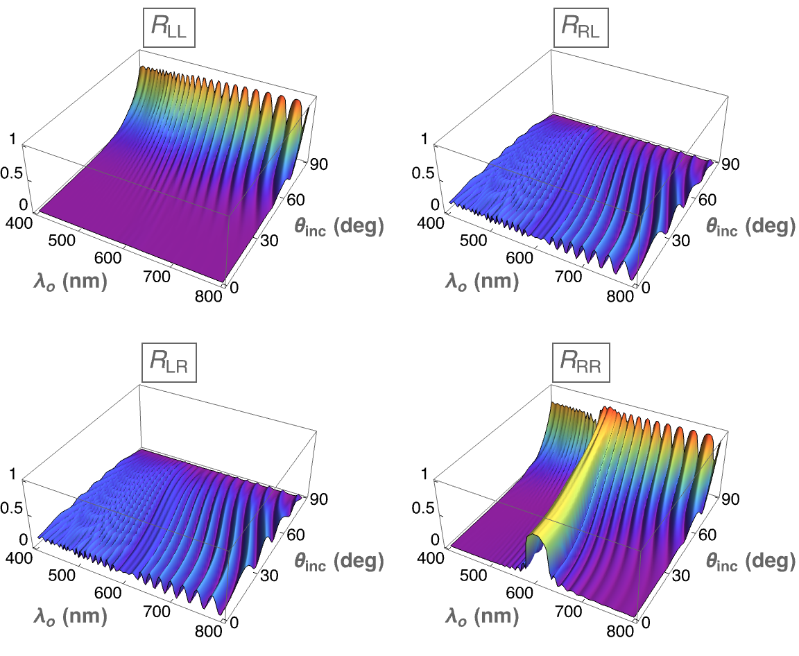
(a) $h=1$, $\theta_{\rm inc}\in[0^{\circ},90^{\circ})$, and $\psi=0^{\circ}$

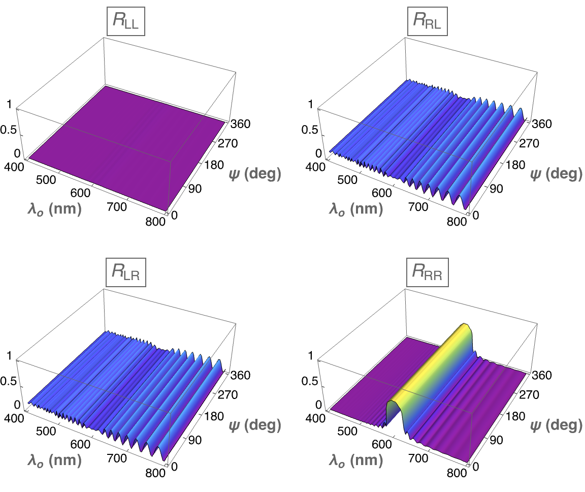
(b) $h=1$, $\theta_{\rm inc}=0^{\circ}$, and $\psi\in[0^{\circ},360^{\circ})$

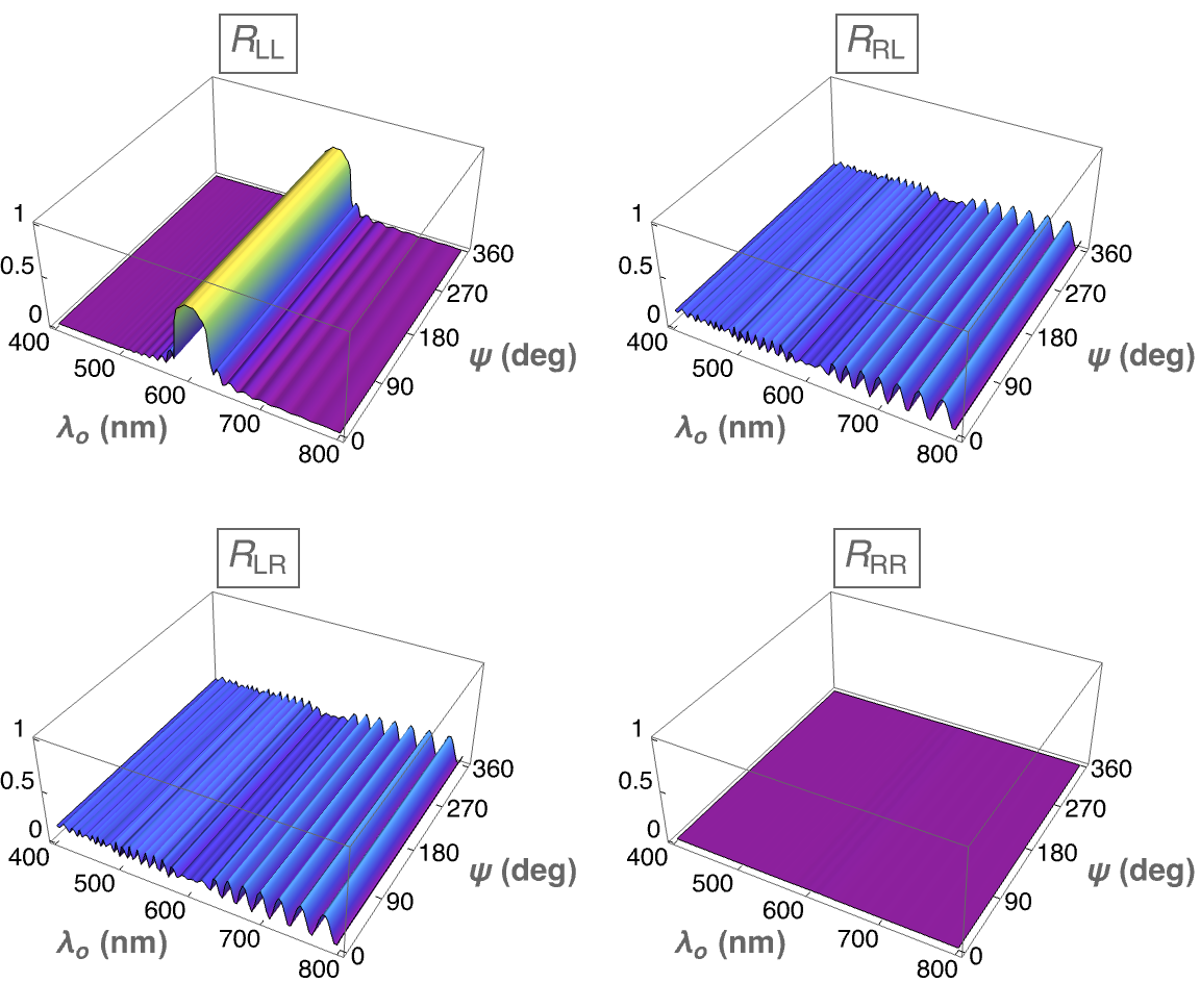
(d) $h=-1$, $\theta_{\rm inc}=0^{\circ}$, and $\psi\in[0^{\circ},360^{\circ})$

Figure 1: Spectral variations of circular reflectances $R_{\mu\nu}(\lambda_{\scriptscriptstyle 0},\theta_{\rm inc},\psi)$, $\mu\in\left\{\rm L,R\right\}$ and $\nu\in\left\{\rm L,R\right\}$, when (a,b) $h=1$ and (c,d) $h=-1$. (a,c) $\theta_{\rm inc}\in[0^{\circ},90^{\circ})$ and $\psi=0^{\circ}$; (b,d) $\theta_{\rm inc}=0^{\circ}$ and $\psi\in[0^{\circ},360^{\circ})$.

————————————————————————————————-

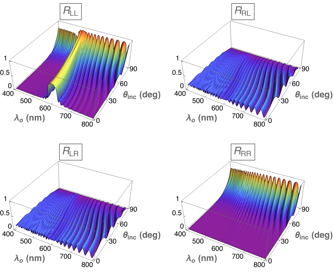
(c) $h=-1$, $\theta_{\rm inc}\in[0^{\circ},90^{\circ})$, and $\psi=0^{\circ}$

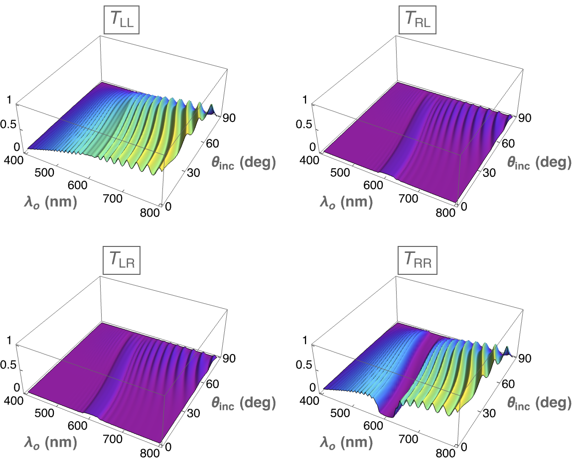
(a) $h=1$, $\theta_{\rm inc}\in[0^{\circ},90^{\circ})$, and $\psi=0^{\circ}$

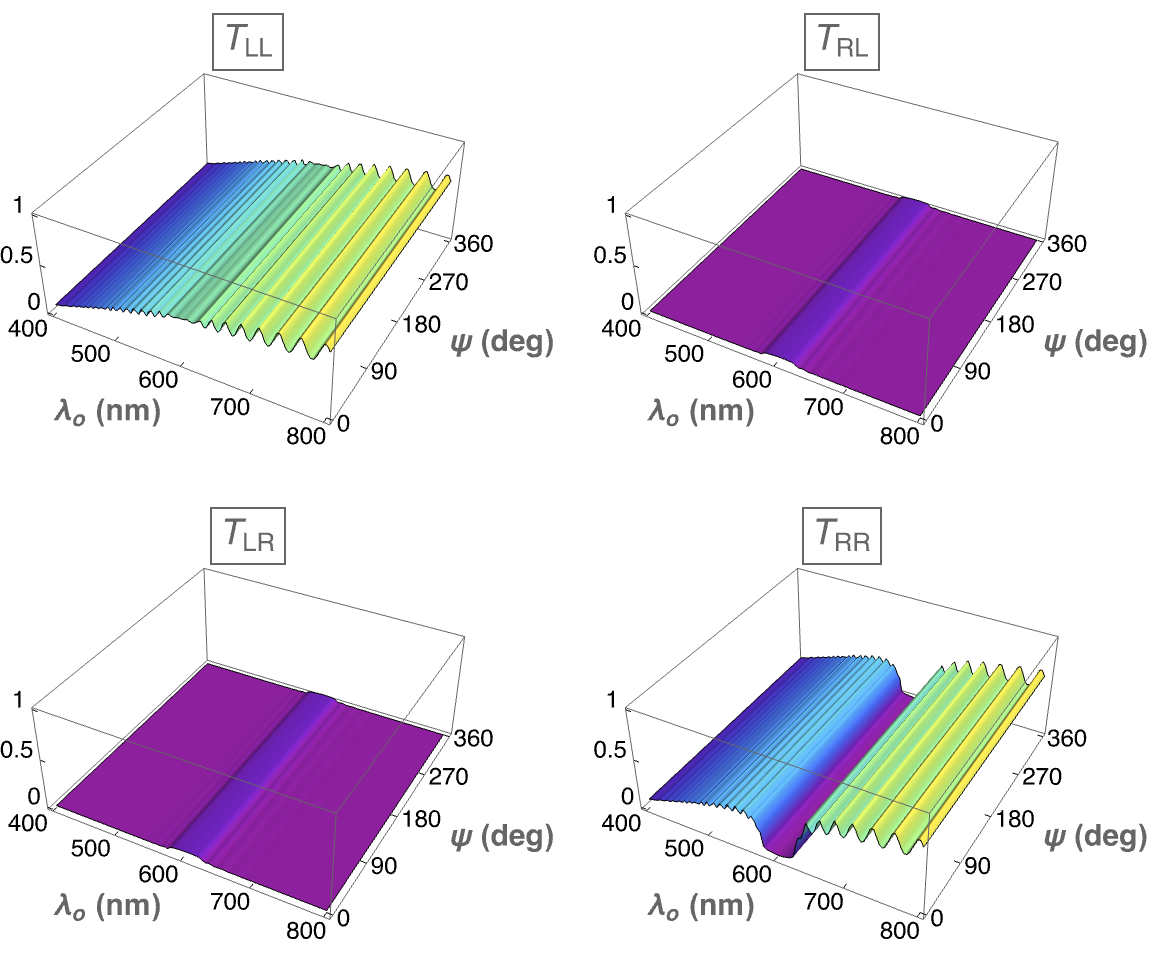
(b) $h=1$, $\theta_{\rm inc}=0^{\circ}$, and $\psi\in[0^{\circ},360^{\circ})$

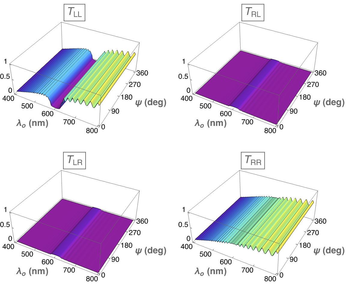
(d) $h=-1$, $\theta_{\rm inc}=0^{\circ}$, and $\psi\in[0^{\circ},360^{\circ})$

Figure 2: Spectral variations of circular transmittances $T_{\mu\nu}(\lambda_{\scriptscriptstyle 0},\theta_{\rm inc},\psi)$, $\mu\in\left\{\rm L,R\right\}$ and $\nu\in\left\{\rm L,R\right\}$, when (a,b) $h=1$ and (c,d) $h=-1$. (a,c) $\theta_{\rm inc}\in[0^{\circ},90^{\circ})$ and $\psi=0^{\circ}$; (b,d) $\theta_{\rm inc}=0^{\circ}$ and $\psi\in[0^{\circ},360^{\circ})$.

————————————————————————————————-

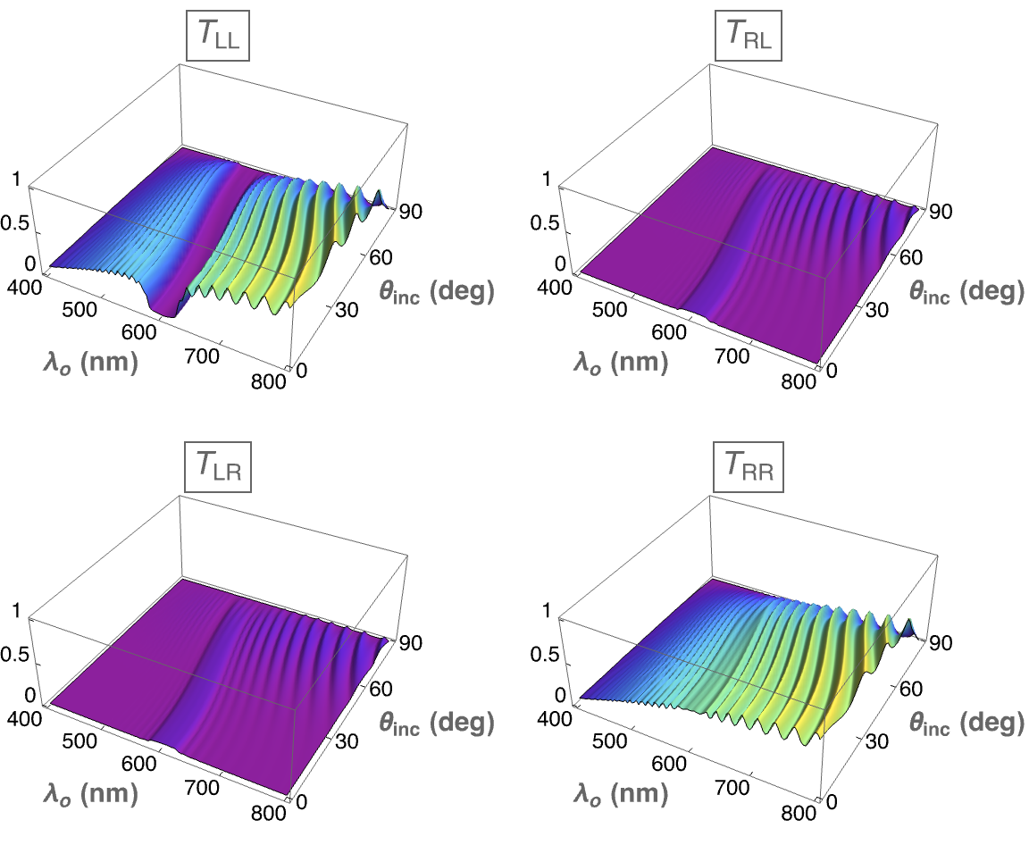
(c) $h=-1$, $\theta_{\rm inc}\in[0^{\circ},90^{\circ})$, and $\psi=0^{\circ}$

3.2 Linear remittances

The square of the magnitude of a linear reflection or transmission coefficient is the corresponding linear reflectance or transmittance; thus, $R_{\rm sp}=|r_{\rm sp}|^{2}\in[0,1]$ is the linear reflectance corresponding to the linear reflection coefficient $r_{\rm sp}$ and $T_{\rm ps}=|t_{\rm ps}|^{2}\in[0,1]$ is the linear transmittance corresponding to the linear transmission coefficient $t_{\rm ps}$, etc. The total linear reflectances are given by

$$\left.\begin{array}[]{l}R_{\rm s}=R_{\rm ss}+R_{\rm ps}\in[0,1]\\[5.0pt] R_{\rm p}=R_{\rm pp}+R_{\rm sp}\in[0,1]\end{array}\right\}$$ (13)

and the total linear transmittances by

$$\left.\begin{array}[]{l}T_{\rm s}=T_{\rm ss}+T_{\rm ps}\in[0,1]\\[5.0pt] T_{\rm p}=T_{\rm pp}+T_{\rm ps}\in[0,1]\end{array}\right\}\,.$$ (14)

The inequalities (12) still hold with $\ell\in\left\{{\rm s,p}\right\}$ and convert to equalities only if the SCM is non-dissipative at a particular frequency of interest.

Linear reflectances can be written in terms of circular reflectances [10]. Therefore, the circular Bragg regime is evident in the spectral variations of both co-polarized linear reflectances as a medium-reflectance ridge and in the spectral variations of both cross-polarized reflectances as a low-reflectance ridge [20, 11], in Fig. 3 for both $h=1$ and $h=-1$. For fixed $\psi$, the ridge curves towards shorter wavelengths as $\theta_{\rm inc}$ increases. For fixed $\theta_{\rm inc}$, the low-reflectance ridge in the plots of $R_{\rm ps}$ and $R_{\rm sp}$ is more or less invariant with respect to $\psi$; but the medium-reflectance ridge in the plots of $R_{\rm ss}$ and $R_{\rm pp}$ has two periods of undulations.

Linear transmittances can be written in terms of circular transmittances [10, 22]. The spectral variations of both co-polarized linear transmittances exhibit a medium-transmittance trough and both cross-polarized linear transmittances show a low-reflectance ridge [20, 11], in Fig. 4 for both $h=1$ and $h=-1$. Indicative of the circular Bragg phenomenon, these features curve towards shorter wavelengths as $\theta_{\rm inc}$ increases when $\psi$ is held fixed. For fixed $\theta_{\rm inc}$ but variable $\psi$, the low-transmittance ridge in the plots of $T_{\rm ps}$ and $T_{\rm sp}$ and the medium-transmittance trough in the plots of $T_{\rm ss}$ and $T_{\rm pp}$ have two periods of undulations.

(a) $h=1$, $\theta_{\rm inc}\in[0^{\circ},90^{\circ})$, and $\psi=0^{\circ}$

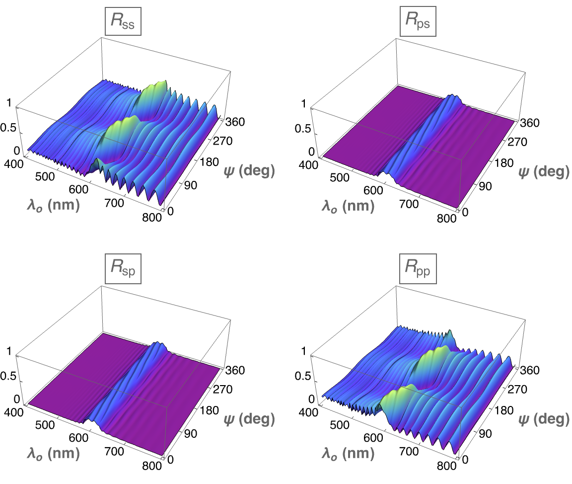
(b) $h=1$, $\theta_{\rm inc}=0^{\circ}$, and $\psi\in[0^{\circ},360^{\circ})$

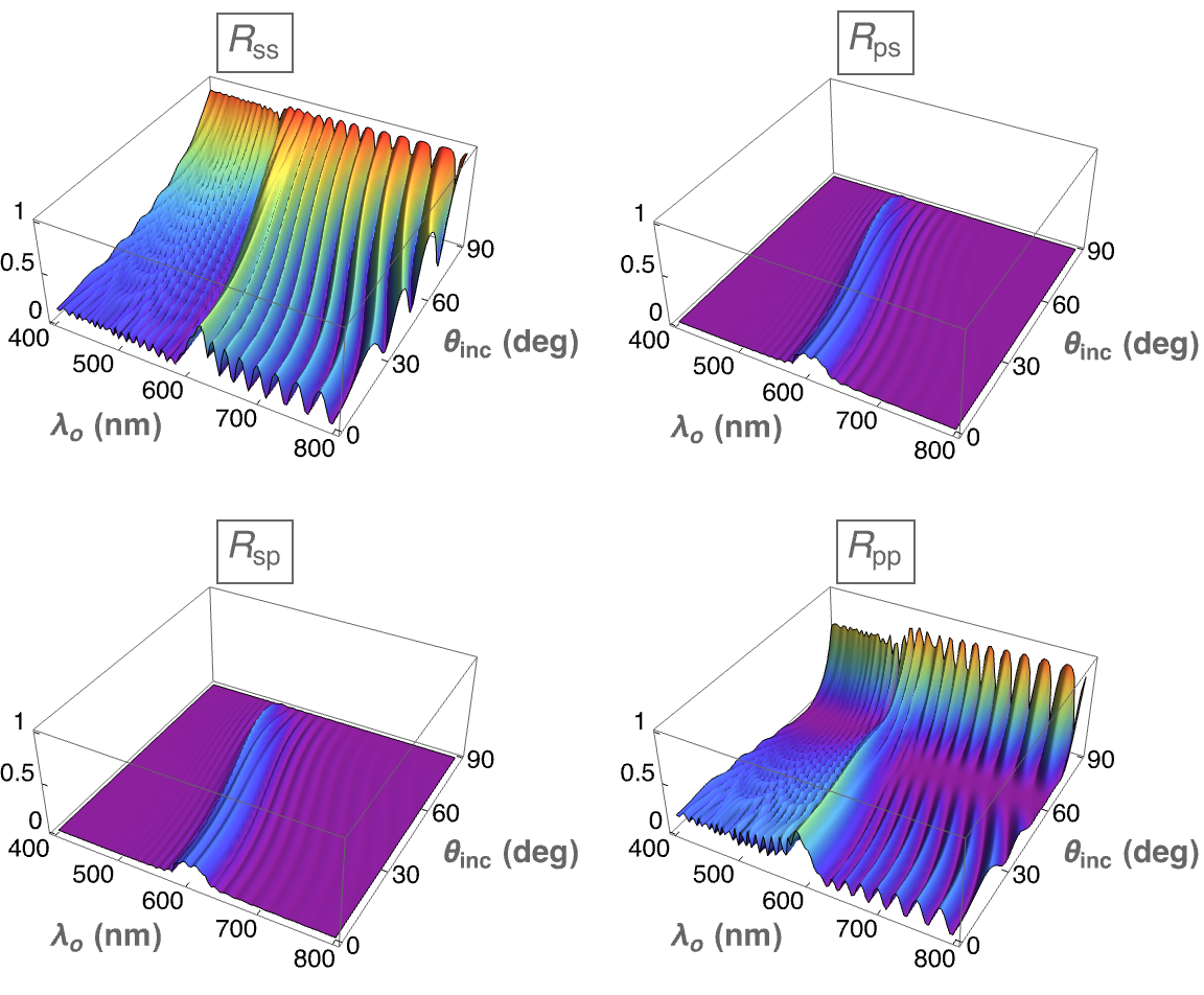
(c) $h=-1$, $\theta_{\rm inc}\in[0^{\circ},90^{\circ})$, and $\psi=0^{\circ}$

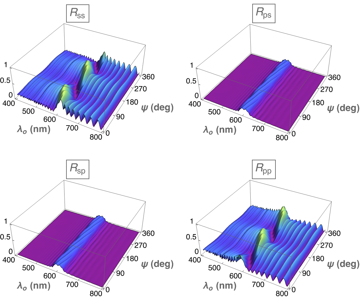
(d) $h=-1$, $\theta_{\rm inc}=0^{\circ}$, and $\psi\in[0^{\circ},360^{\circ})$

Figure 3: Spectral variations of linear reflectances $R_{\mu\nu}(\lambda_{\scriptscriptstyle 0},\theta_{\rm inc},\psi)$, $\mu\in\left\{\rm s,p\right\}$ and $\nu\in\left\{\rm s,p\right\}$, when (a,b) $h=1$ and (c,d) $h=-1$. (a,c) $\theta_{\rm inc}\in[0^{\circ},90^{\circ})$ and $\psi=0^{\circ}$; (b,d) $\theta_{\rm inc}=0^{\circ}$ and $\psi\in[0^{\circ},360^{\circ})$.

(a) $h=1$, $\theta_{\rm inc}\in[0^{\circ},90^{\circ})$, and $\psi=0^{\circ}$

(b) $h=1$, $\theta_{\rm inc}=0^{\circ}$, and $\psi\in[0^{\circ},360^{\circ})$

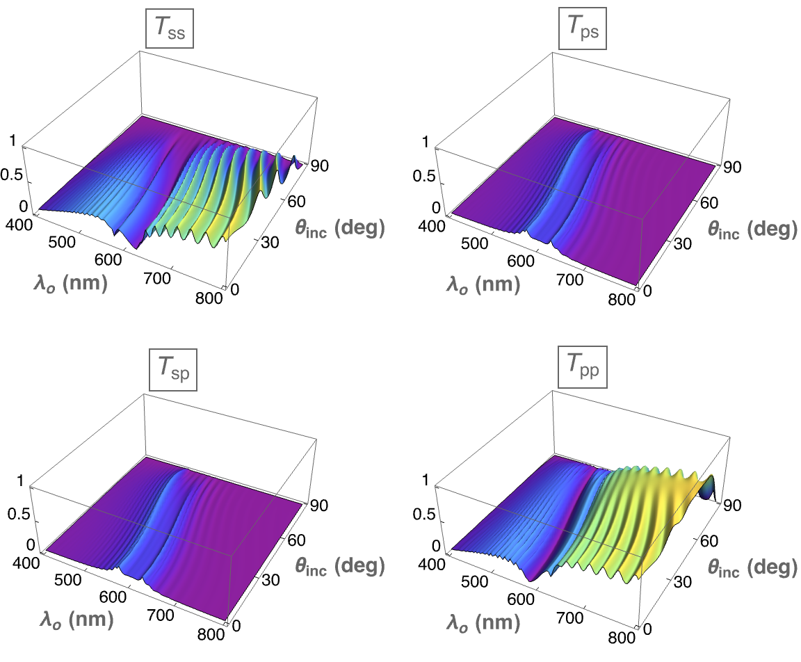
(c) $h=-1$, $\theta_{\rm inc}\in[0^{\circ},90^{\circ})$, and $\psi=0^{\circ}$

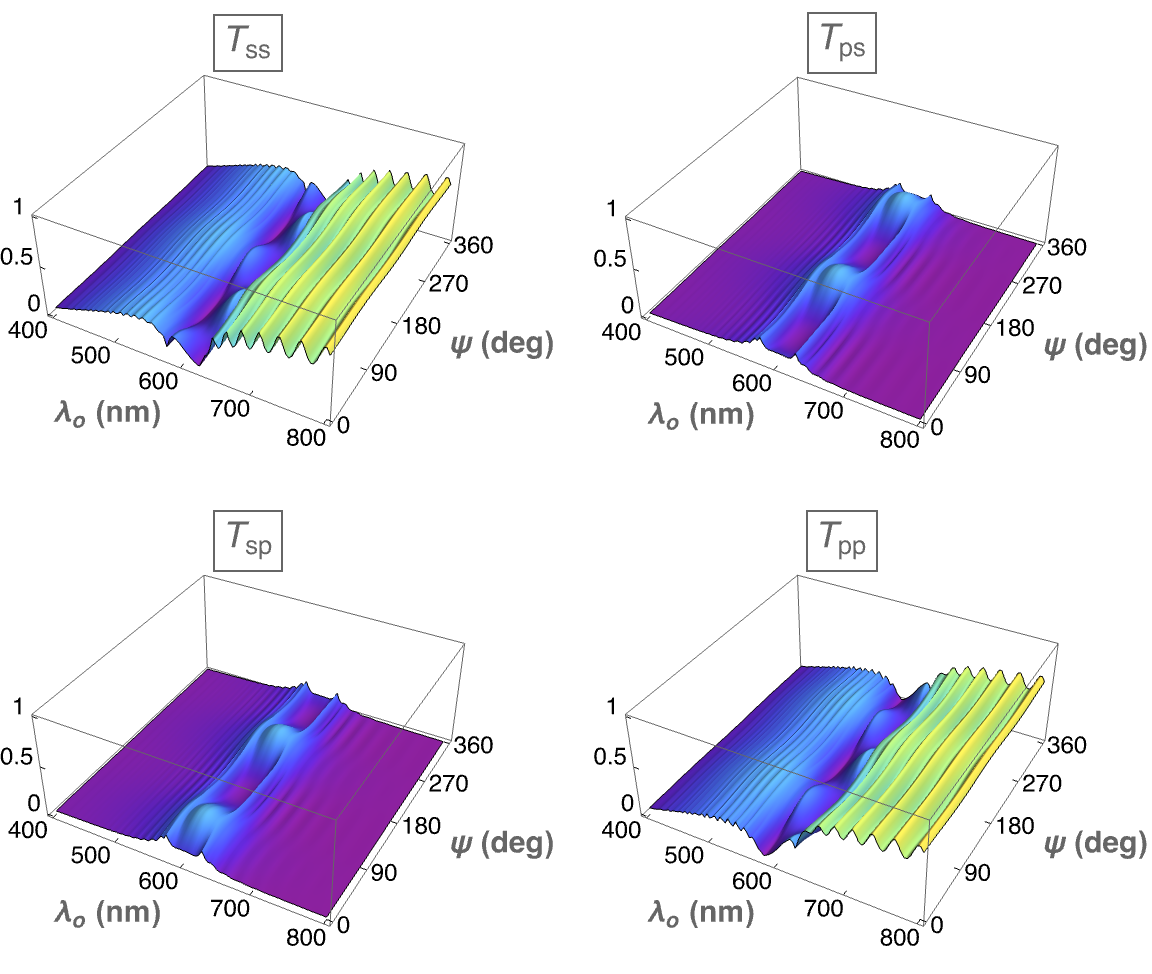
(d) $h=-1$, $\theta_{\rm inc}=0^{\circ}$, and $\psi\in[0^{\circ},360^{\circ})$

Figure 4: Spectral variations of linear transmittances $T_{\mu\nu}(\lambda_{\scriptscriptstyle 0},\theta_{\rm inc},\psi)$, $\mu\in\left\{\rm s,p\right\}$ and $\nu\in\left\{\rm s,p\right\}$, when (a,b) $h=1$ and (c,d) $h=-1$. (a,c) $\theta_{\rm inc}\in[0^{\circ},90^{\circ})$ and $\psi=0^{\circ}$; (b,d) $\theta_{\rm inc}=0^{\circ}$ and $\psi\in[0^{\circ},360^{\circ})$.

3.3 Circular and linear dichroisms

With

$$\left.\begin{array}[]{l}A_{\rm L}=1-\left(R_{\rm L}+T_{\rm L}\right)\in[0,1]\\[5.0pt] A_{\rm R}=1-\left(R_{\rm R}+T_{\rm R}\right)\in[0,1]\end{array}\right\}$$ (15)

as the circular absorptances,

$${CD}_{\rm tru}=\sqrt{A_{\rm R}}-\sqrt{A_{\rm L}}\in[-1,1]$$ (16)

is the true circular dichroism which quantitates the circular-polarization-dependence of absorption. The apparent circular dichroism

$${CD}_{\rm app}=\sqrt{T_{\rm R}}-\sqrt{T_{\rm L}}\in[-1,1]$$ (17)

is a measure of the circular-polarization-state-dependence of transmission [11]. Whereas ${CD}_{\rm app}$ may not equal zero for a non-dissipative SCM, ${CD}_{\rm tru}$ must be.

Figure 5 contains plots of the spectral variations of both ${CD}_{\rm app}$ and ${CD}_{\rm tru}$ in relation to the direction of plane-wave incidence. The circular Bragg phenomenon is evident as a trough in all plots of ${CD}_{\rm app}$ and ${CD}_{\rm tru}$ for $h=1$, and as a ridge in all plots of ${CD}_{\rm app}$ and ${CD}_{\rm tru}$ for $h=-1$. Furthermore, the quantities $h{CD}_{\rm app}$ and $h{CD}_{\rm tru}$ are invariant if the sign of $h$ is changed. These features curve towards shorter wavelengths as $\theta_{\rm inc}$ increases while $\psi$ is held fixed, as has been experimentally verified [11]. For normal incidence (i.e., $\theta_{\rm inc}=0^{\circ}$), the effect of $\psi$ is minimal.

Similarly to the circular absorptances,

$$\left.\begin{array}[]{l}A_{\rm s}=1-\left(R_{\rm ss}+T_{\rm s}\right)\in[0,1]\\[5.0pt] A_{\rm p}=1-\left(R_{\rm p}+T_{\rm p}\right)\in[0,1]\end{array}\right\}$$ (18)

are the linear absorptances. The true linear dichroism is defined as [11]

$${LD}_{\rm tru}=\sqrt{A_{\rm s}}-\sqrt{A_{\rm p}}\in[-1,1]$$ (19)

and the apparent linear dichroism as

$${LD}_{\rm app}=\sqrt{T_{\rm s}}-\sqrt{T_{\rm p}}\in[-1,1]\,.$$ (20)

Whereas ${LD}_{\rm tru}\equiv 0$ for a non-dissipative SCM, ${LD}_{\rm app}$ may not be null valued.

Figure 5 also contains plots of the spectral variations of both ${LD}_{\rm app}$ and ${LD}_{\rm tru}$ in relation to the direction of plane-wave incidence. The circular Bragg phenomenon is featured in all plots. For fixed $\psi$, the feature curves towards shorter wavelengths as $\theta_{\rm inc}$ increases, which has been experimentally verified [11]. For normal incidence, the feature has two undulations with increasing $\psi$, and the replacement $h\to-h$ affects both ${LD}_{\rm app}$ and ${LD}_{\rm tru}$ non-trivially.

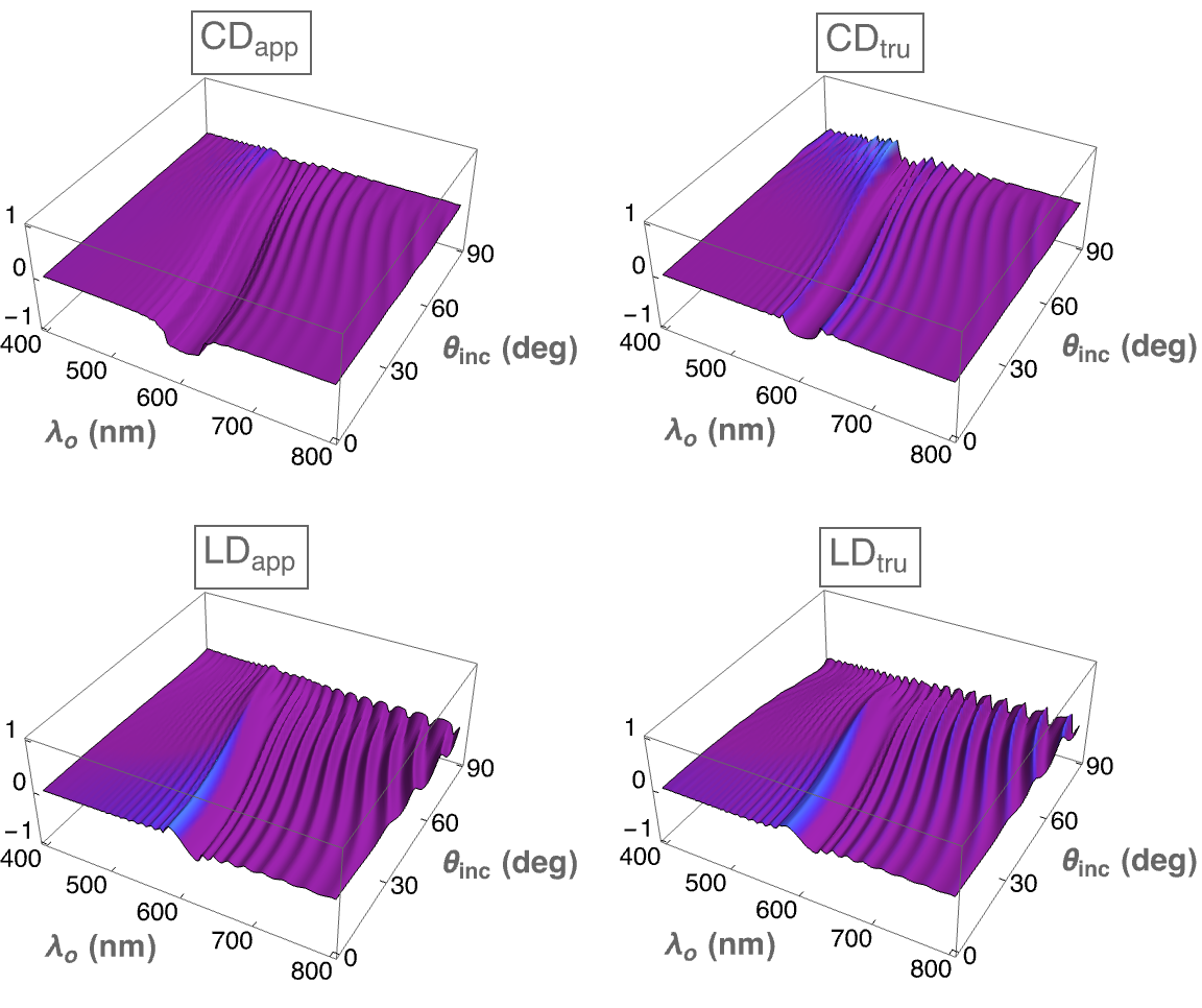
(a) $h=1$, $\theta_{\rm inc}\in[0^{\circ},90^{\circ})$, and $\psi=0^{\circ}$

(b) $h=1$, $\theta_{\rm inc}=0^{\circ}$, and $\psi\in[0^{\circ},360^{\circ})$

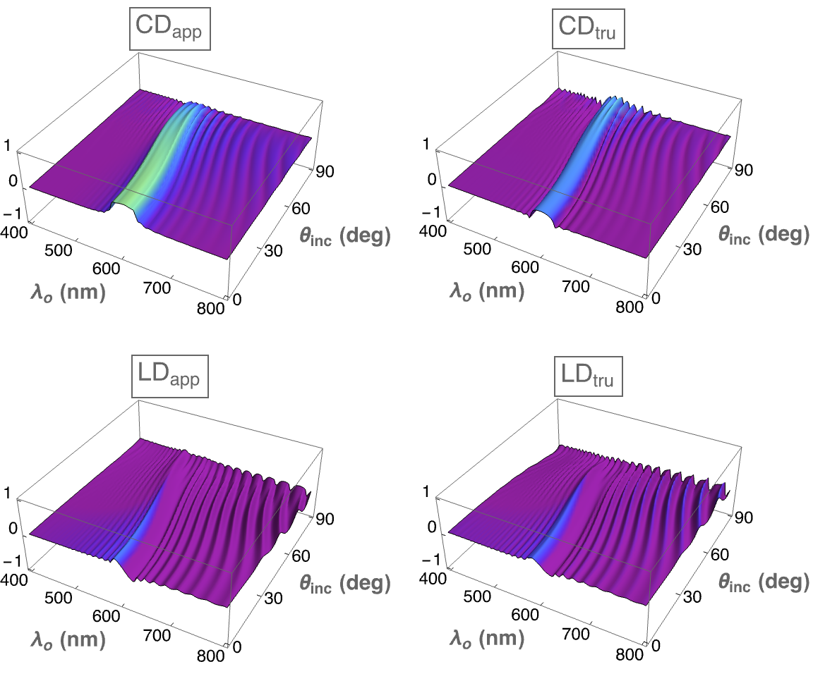
(c) $h=-1$, $\theta_{\rm inc}\in[0^{\circ},90^{\circ})$, and $\psi=0^{\circ}$

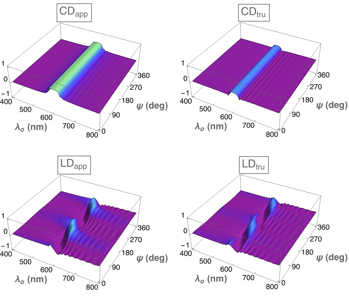
(d) $h=-1$, $\theta_{\rm inc}=0^{\circ}$, and $\psi\in[0^{\circ},360^{\circ})$

Figure 5: Spectral variations of apparent circular dichroism ${CD}_{\rm app}(\lambda_{\scriptscriptstyle 0},\theta_{\rm inc},\psi)$, true circular dichroism ${CD}_{\rm tru}(\lambda_{\scriptscriptstyle 0},\theta_{\rm inc},\psi)$, apparent linear dichroism ${LD}_{\rm app}(\lambda_{\scriptscriptstyle 0},\theta_{\rm inc},\psi)$, and true linear dichroism ${LD}_{\rm tru}(\lambda_{\scriptscriptstyle 0},\theta_{\rm inc},\psi)$, when (a,b) $h=1$ and (c,d) $h=-1$. (a,c) $\theta_{\rm inc}\in[0^{\circ},90^{\circ})$ and $\psi=0^{\circ}$; (b,d) $\theta_{\rm inc}=0^{\circ}$ and $\psi\in[0^{\circ},360^{\circ})$.

4 Phase-dependent quantities

4.1 Ellipticity and optical rotation

The most general plane wave in free space is elliptically polarized [41]. Signed ellipticity functions

$$\left.\begin{array}[]{l}EF^{\rm inc}=\displaystyle{-2\,\frac{{\rm Im}\left({a_{\rm s}}a_{\rm p}^{*}\right)}{|{a_{\rm s}}|^{2}+|{a_{\rm p}}|^{2}}}\\[10.0pt] EF^{\rm ref}=\displaystyle{-2\,\frac{{\rm Im}\left({r_{\rm s}}r_{\rm p}^{*}\right)}{|{r_{\rm s}}|^{2}+|{r_{\rm p}}|^{2}}}\\[10.0pt] EF^{\rm tr}=\displaystyle{-2\,\frac{{\rm Im}\left(t_{\rm s}t_{\rm p}^{*}\right)}{|t_{\rm s}|^{2}+|t_{\rm p}|^{2}}}\end{array}\right\}\,$$ (21)

characterize the shapes of the vibration ellipses of the incident, reflected, and transmitted plane waves.

Note that $EF^{\ell}\in[-1,1]$, $\ell\in\left\{{\rm inc},\,{\rm ref},\,{\rm tr}\right\}$. The magnitude of $EF^{\ell}$ is the ellipticity of the plane wave labelled $\ell$. The vibration ellipse simplifies to a circle when $\big{|}EF^{\ell}\big{|}=1$ (circular polarization state), and it degenerates into a straight line when $EF^{\ell}=0$ (linear polarization state). The plane wave is left-handed for $EF^{\ell}>0$ and right-handed for $EF^{\ell}<0$.

The major axes of the vibration ellipses of the incident and the reflected/transmitted plane wave may not coincide, the angular offset between the two major axes known as optical rotation. The auxiliary vectors [10]

$$\left.\begin{array}[]{l}{\bf F}^{\rm inc}=\left\{1+\left[1-\left(EF^{\rm inc}\right)^{2}\right]^{1/2}\right\}\,{\rm Re}\left({a_{\rm s}}{\bf s}+{a_{\rm p}}{\bf p}_{+}\right)+EF^{\rm inc}\,{\rm Im}\left({a_{\rm s}}{\bf p}_{+}-{a_{\rm p}}{\bf s}\right)\\[8.0pt] {\bf F}^{\rm ref}=\left\{1+\left[1-\left(EF^{\rm ref}\right)^{2}\right]^{1/2}\right\}\,{\rm Re}\left({r_{\rm s}}{\bf s}+{r_{\rm p}}{\bf p}_{-}\right)+EF^{\rm ref}\,{\rm Im}\left({r_{\rm s}}{\bf p}_{-}-{r_{\rm p}}{\bf s}\right)\\[8.0pt] {\bf F}^{\rm tr}=\left\{1+\left[1-\left(EF^{\rm tr}\right)^{2}\right]^{1/2}\right\}\,{\rm Re}\left({t_{\rm s}}{\bf s}+{t_{\rm p}}{\bf p}_{+}\right)+EF^{\rm tr}\,{\rm Im}\left({t_{\rm s}}{\bf p}_{+}-{t_{\rm p}}{\bf s}\right)\end{array}\right\}\,$$ (22)

are parallel to the major axes of the respective vibration ellipses. Therefrom, the angles $\tau^{\rm inc}$, $\tau^{\rm ref}$, and $\tau^{\rm tr}$ are calculated using the following expressions:

$$\left.\begin{array}[]{ll}\cos\tau^{\ell}=\left({{\bf F}^{\ell}\mbox{ \tiny{${}^{\bullet}$} }{\bf s}}\right)/{\big{|}{\bf F}^{\ell}\big{|}}\,,&\quad\ell\in\left\{{\rm inc},\,{\rm ref},\,{\rm tr}\right\}\\[5.0pt] \sin\tau^{\ell}=\left({{\bf F}^{\ell}\mbox{ \tiny{${}^{\bullet}$} }{\bf p}_{+}}\right)/{\big{|}{\bf F}^{\ell}\big{|}}\,,&\quad\ell\in\left\{{\rm inc},\,{\rm tr}\right\}\\[5.0pt] \sin\tau^{\rm ref}=\left({{\bf F}^{\rm ref}\mbox{ \tiny{${}^{\bullet}$} }{\bf p}_{-}}\right)/{\big{|}{\bf F}^{\rm ref}\big{|}}\end{array}\right\}\,.$$ (23)

The optical rotation of the reflected/transmitted plane wave then is the angle

$$OR^{\ell}=\left\{\begin{array}[]{lll}\tau^{\ell}-\tau^{\rm inc}+\pi\,,&{\rm if}\,-\pi\leq\tau^{\ell}-\tau^{\rm inc}\leq-\pi/2\,,\\[5.0pt] \tau^{\ell}-\tau^{\rm inc}\,,&{\rm if}\,\big{|}\tau^{\ell}-\tau^{\rm inc}\big{|}<\pi/2\,,\\[5.0pt] \tau^{\ell}-\tau^{\rm inc}-\pi\,,&{\rm if}\,\pi/2\leq\tau^{\ell}-\tau^{\rm inc}\leq\pi\,,\end{array}\right.\,,\quad\ell\in\left\{{\rm ref},\,{\rm tr}\right\}\,.$$ (24)

The ellipticity function of the reflected/transmitted plane wave is denoted by $EF^{\ell}_{\rm s}$ and $EF^{\ell}_{\rm p}$, respectively, and the optical rotation of the reflected/transmitted plane wave is denoted by $OR^{\ell}_{\rm s}$ and $OR^{\ell}_{\rm p}$, respectively, for incident perpendicular-polarized and parallel-polarized plane waves, $\ell\in\left\{{\rm ref},\,{\rm tr}\right\}$.

Figure 6 provides the spectral variations of $EF^{\rm ref}_{\rm s,p}$ and $OR^{\rm ref}_{\rm s,p}$, and Fig. 7 the spectral variations of $EF^{\rm tra}_{\rm s,p}$ and $OR^{\rm tra}_{\rm s,p}$. A feature representing the circular Bragg phenomenon is clearly evident in all 32 plots in the two figures. For fixed $\psi$, the feature curves towards shorter wavelengths as $\theta_{\rm inc}$ increases. For normal incidence, the feature has two undulations with increasing $\psi$. Although measurements of optical rotation and ellipticity of the transmitted plane wave for normal incidence have been reported for over a century [42], comprehensive experimental investigations for oblique incidence are very desirable in the near future.

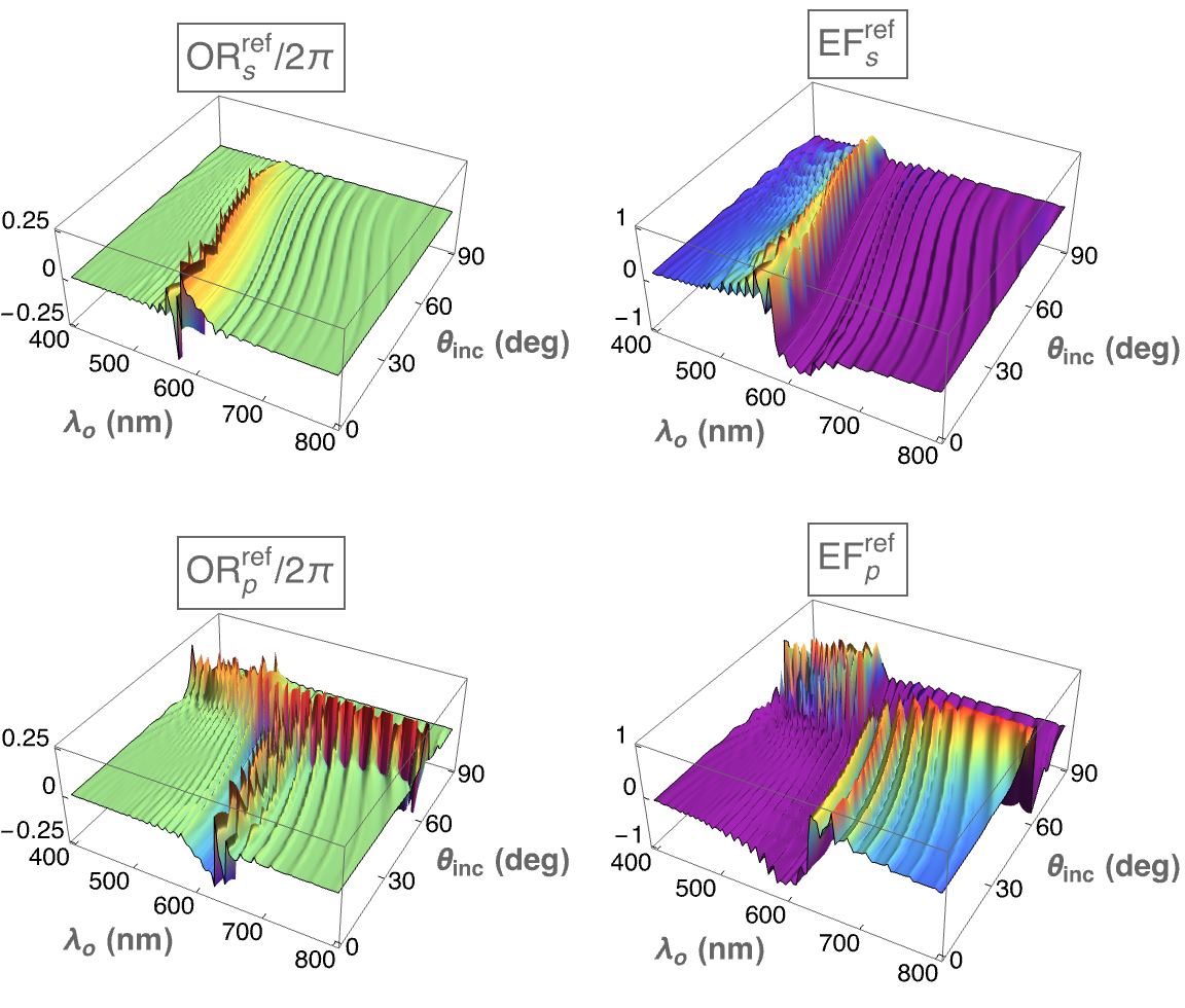
(a) $h=1$, $\theta_{\rm inc}\in[0^{\circ},90^{\circ})$, and $\psi=0^{\circ}$

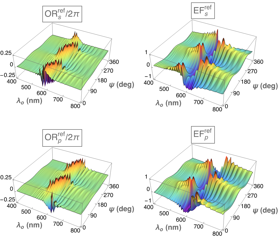
(b) $h=1$, $\theta_{\rm inc}=0^{\circ}$, and $\psi\in[0^{\circ},360^{\circ})$

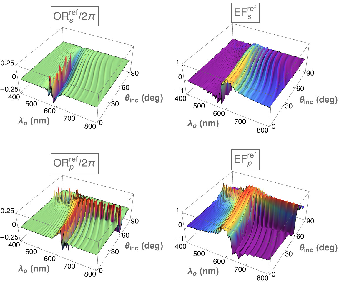
(c) $h=-1$, $\theta_{\rm inc}\in[0^{\circ},90^{\circ})$, and $\psi=0^{\circ}$

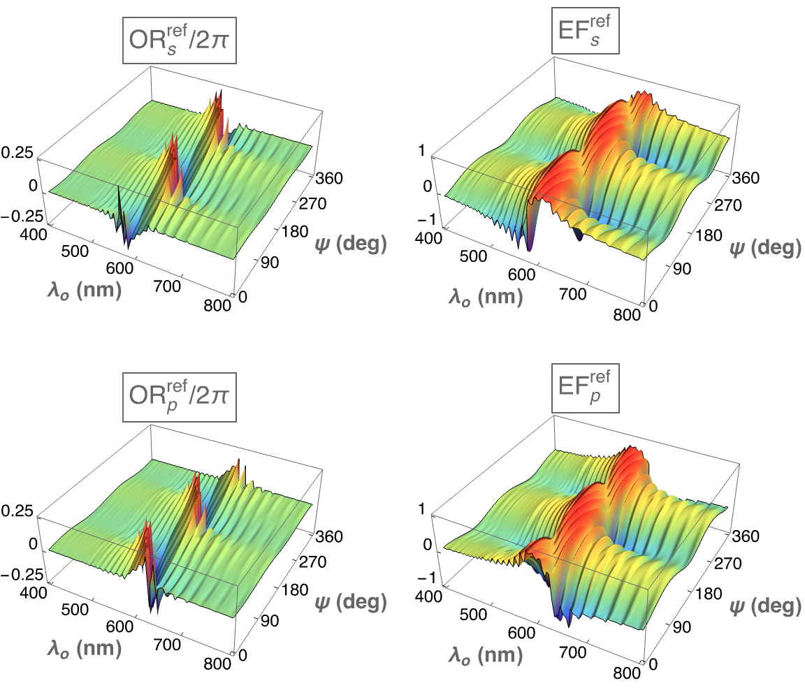
(d) $h=-1$, $\theta_{\rm inc}=0^{\circ}$, and $\psi\in[0^{\circ},360^{\circ})$

Figure 6: Spectral variations of the optical rotation $OR^{\rm ref}_{\mu}(\lambda_{\scriptscriptstyle 0},\theta_{\rm inc},\psi)$ and ellipticity function $EF^{\rm ref}_{\mu}(\lambda_{\scriptscriptstyle 0},\theta_{\rm inc},\psi)$, $\mu\in\left\{s,p\right\}$, of the reflected plane wave, when (a,b) $h=1$ and (c,d) $h=-1$. (a,c) $\theta_{\rm inc}\in[0^{\circ},90^{\circ})$ and $\psi=0^{\circ}$; (b,d) $\theta_{\rm inc}=0^{\circ}$ and $\psi\in[0^{\circ},360^{\circ})$.

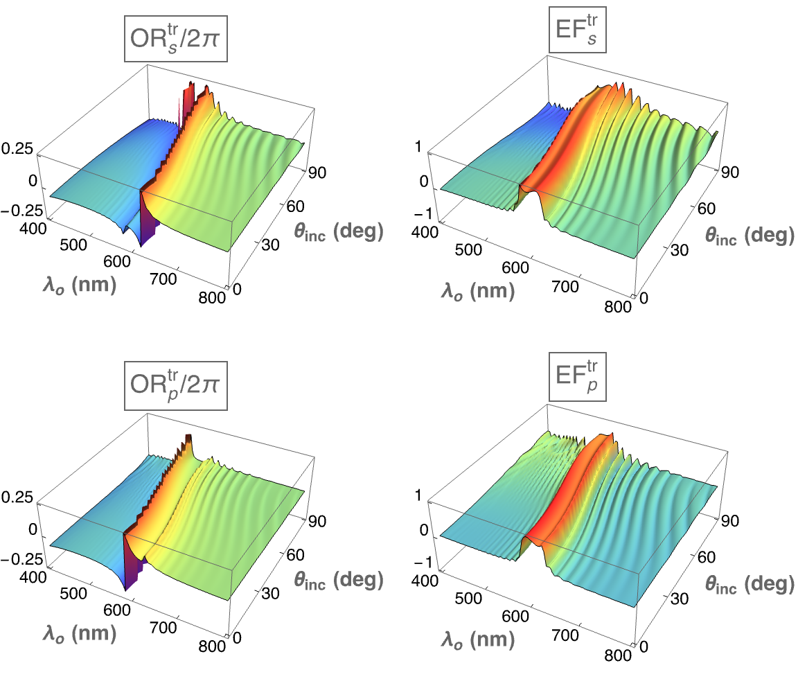
(a) $h=1$, $\theta_{\rm inc}\in[0^{\circ},90^{\circ})$, and $\psi=0^{\circ}$

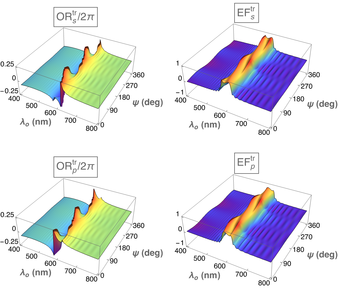
(b) $h=1$, $\theta_{\rm inc}=0^{\circ}$, and $\psi\in[0^{\circ},360^{\circ})$

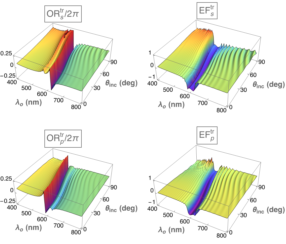
(c) $h=-1$, $\theta_{\rm inc}\in[0^{\circ},90^{\circ})$, and $\psi=0^{\circ}$

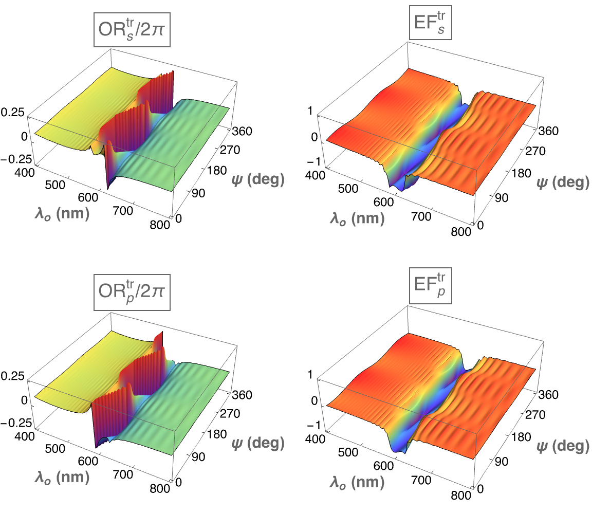
(d) $h=-1$, $\theta_{\rm inc}=0^{\circ}$, and $\psi\in[0^{\circ},360^{\circ})$

Figure 7: Spectral variations of the optical rotation $OR^{\rm tr}_{\mu}(\lambda_{\scriptscriptstyle 0},\theta_{\rm inc},\psi)$ and ellipticity function $EF^{\rm tr}_{\mu}(\lambda_{\scriptscriptstyle 0},\theta_{\rm inc},\psi)$, $\mu\in\left\{s,p\right\}$, of the transmitted plane wave, when (a,b) $h=1$ and (c,d) $h=-1$. (a,c) $\theta_{\rm inc}\in[0^{\circ},90^{\circ})$ and $\psi=0^{\circ}$; (b,d) $\theta_{\rm inc}=0^{\circ}$ and $\psi\in[0^{\circ},360^{\circ})$.

4.2 Geometric phases of reflected and transmitted plane waves

The Stokes parameters of the incident plane wave are given by [44]

$$\left.\begin{array}[]{l}s_{0}^{\rm inc}=|a_{\rm L}|^{2}+|a_{\rm R}|^{2}=|a_{\rm s}|^{2}+|a_{\rm p}|^{2}\\[5.0pt] s_{1}^{\rm inc}=2\,{\rm Re}\left(a_{\rm L}\,a_{\rm R}^{\ast}\right)=|a_{\rm p}|^{2}-|a_{\rm s}|^{2}\\[5.0pt] s_{2}^{\rm inc}=2\,{\rm Im}\left(a_{\rm L}\,a_{\rm R}^{\ast}\right)=2\,{\rm Re}\left(a_{\rm s}\,a_{\rm p}^{\ast}\right)\\[5.0pt] s_{3}^{\rm inc}=|a_{\rm R}|^{2}-|a_{\rm L}|^{2}=2\,{\rm Im}\left(a_{\rm s}\,a_{\rm p}^{\ast}\right)\end{array}\right\}\,.$$ (25)

The Poincaré spinor $\left[{\underline{\phi}}^{\rm inc}\right]$ of the incident plane wave can then be obtained from Eqs. (26) and (27) in the Appendix.

After making the changes $\left\{a_{\rm L}\to r_{\rm L},\,a_{\rm R}\to r_{\rm R},\,a_{\rm s}\to r_{\rm s},\,a_{\rm p}\to r_{\rm p}\right\}$, Eqs. (25) can be used to determine the Stokes parameters $s_{0}^{\rm ref}$, $s_{1}^{\rm ref}$, $s_{2}^{\rm ref}$, and $s_{3}^{\rm ref}$ of the reflected plane wave, and the Poincaré spinor $\left[{\underline{\phi}}^{\rm ref}\right]$ of the reflected plane wave can then be obtained from Eqs. (26) and (27). Calculation of the Poincaré spinor $\left[{\underline{\phi}}^{\rm tr}\right]$ of the transmitted plane wave follows the same route.

Thereafter, the reflection-mode geometric phase $\Phi^{\rm ref}_{\ell}$ and the transmission-mode geometric phase $\Phi^{\rm tr}_{\ell}$, $\ell\in\left\{s,p,R,L\right\}$, can be calculated with respect to the incident plane wave using Eq. (28) in available in the Appendix. The subscript $\ell$ in both quantities indicates the polarization state of the incident plane wave: perpendicular ($s$), parallel ($p$), left-circular ($L$), or right-circular ($R$).

Note that $\Phi_{\rm R}^{\rm ref}=\Phi_{\rm R}^{\rm tr}\equiv 0$ because of the structure of $\left[{\underline{\phi}}^{\rm inc}\right]$ for an incident RCP plane wave [22, 23]. The other six geometric phases $\Phi^{\rm ref}_{\ell}$ and $\Phi^{\rm tr}_{\ell}$, $\ell\in\left\{s,p,L\right\}$, are generally non-zero in Figs. 8–11; furthermore, their spectral dependencies have some resemblance to those of the corresponding total remittances defined in Eqs. (10), (11), (13), and (14). Indeed, a feature representing the circular Bragg phenomenon is clearly evident in the plots of $\Phi^{\rm ref}_{\ell}$ and $\Phi^{\rm tr}_{\ell}$, $\ell\in\left\{s,p,L\right\}$. The feature curves towards shorter wavelengths as $\theta_{\rm inc}$ increases while $\psi$ is fixed, and the feature has two undulations with increasing $\psi$ for normal incidence.

Although the geometric phase of the transmitted plane wave has been measured for normal incidence on a chiral sculptured thin film [21], that was done only at a single value of $\lambda_{\scriptscriptstyle 0}$, that too in the long-wavelength neighborhood of the circular Bragg regime. Hopefully, experimental verification of the features evident in Figs. 8–11 will be carried out soon and the role of structural handedness clarified.

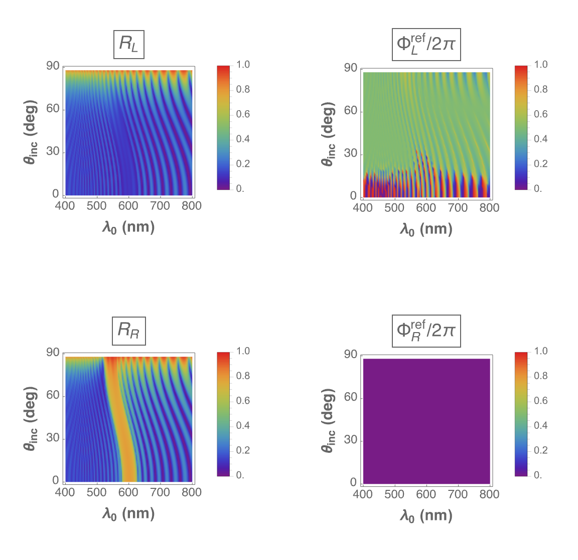
(a) $h=1$, $\theta_{\rm inc}\in[0^{\circ},90^{\circ})$, and $\psi=0^{\circ}$

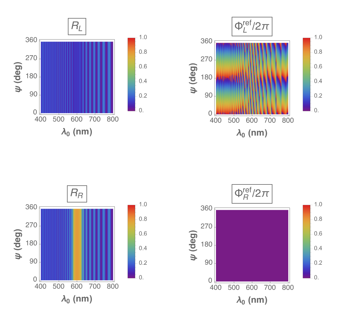
(b) $h=1$, $\theta_{\rm inc}=0^{\circ}$, and $\psi\in[0^{\circ},360^{\circ})$

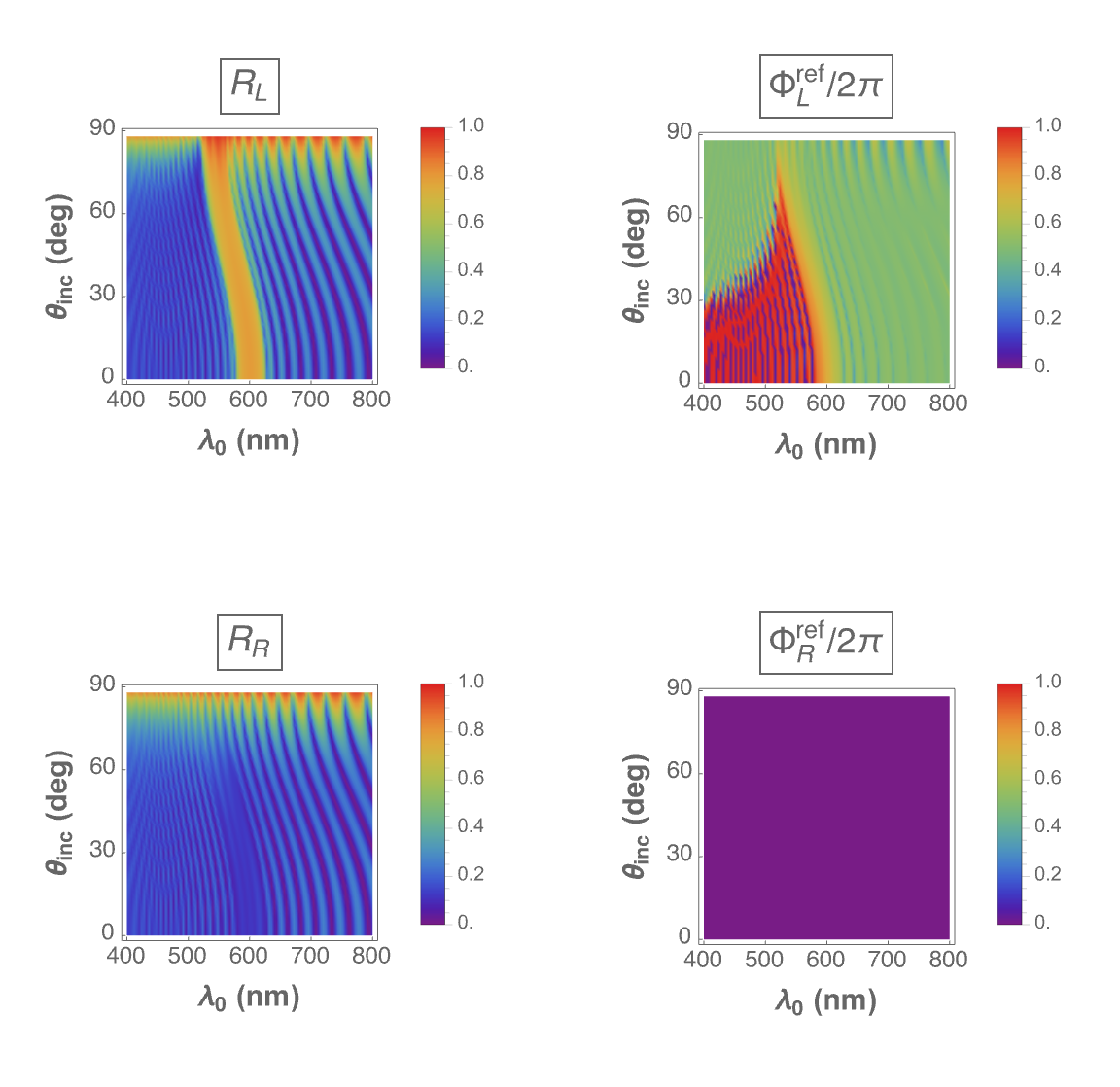
(c) $h=-1$, $\theta_{\rm inc}\in[0^{\circ},90^{\circ})$, and $\psi=0^{\circ}$

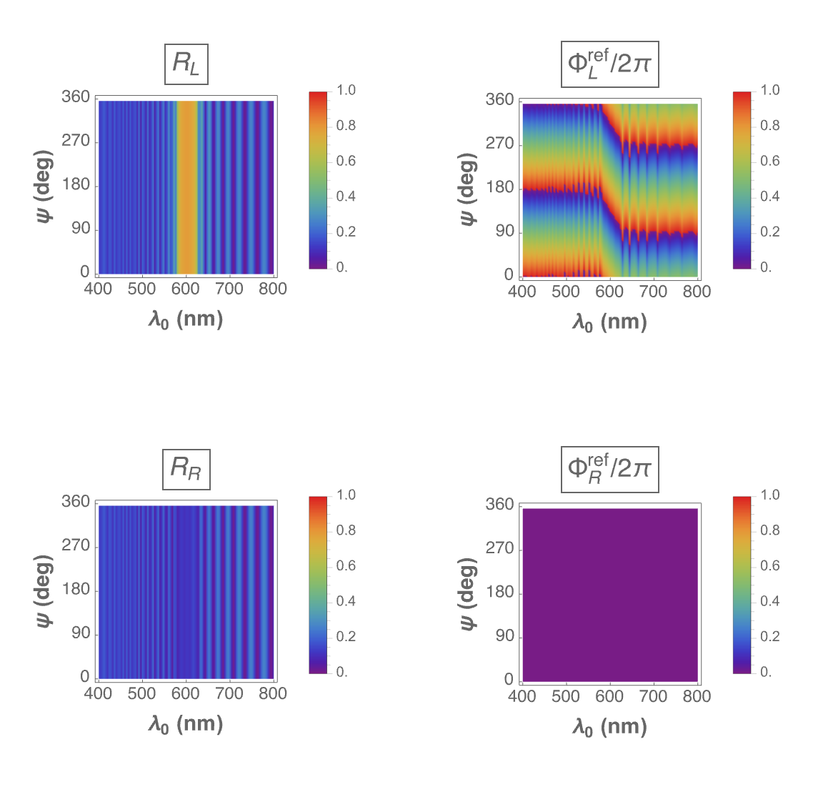
(d) $h=-1$, $\theta_{\rm inc}=0^{\circ}$, and $\psi\in[0^{\circ},360^{\circ})$

Figure 8: Spectral variations of the total circular reflectance $R_{\mu}(\lambda_{\scriptscriptstyle 0},\theta_{\rm inc},\psi)$ and reflection-mode geometric phase $\Phi^{\rm ref}_{\mu}(\lambda_{\scriptscriptstyle 0},\theta_{\rm inc},\psi)$, $\mu\in\left\{L,R\right\}$, when (a,b) $h=1$ and (c,d) $h=-1$. (a,c) $\theta_{\rm inc}\in[0^{\circ},90^{\circ})$ and $\psi=0^{\circ}$; (b,d) $\theta_{\rm inc}=0^{\circ}$ and $\psi\in[0^{\circ},360^{\circ})$.

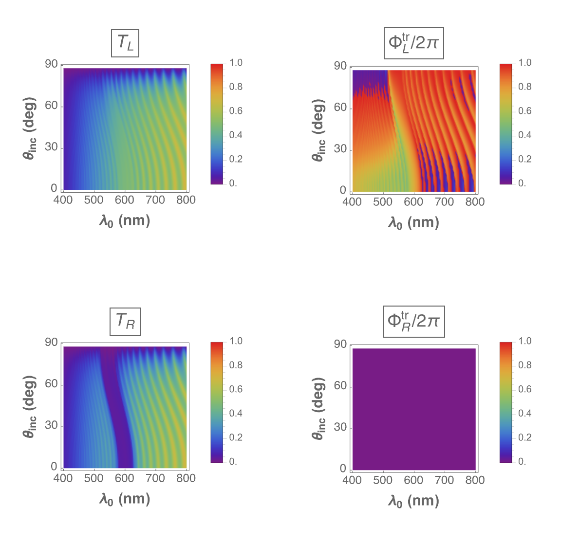
(a) $h=1$, $\theta_{\rm inc}\in[0^{\circ},90^{\circ})$, and $\psi=0^{\circ}$

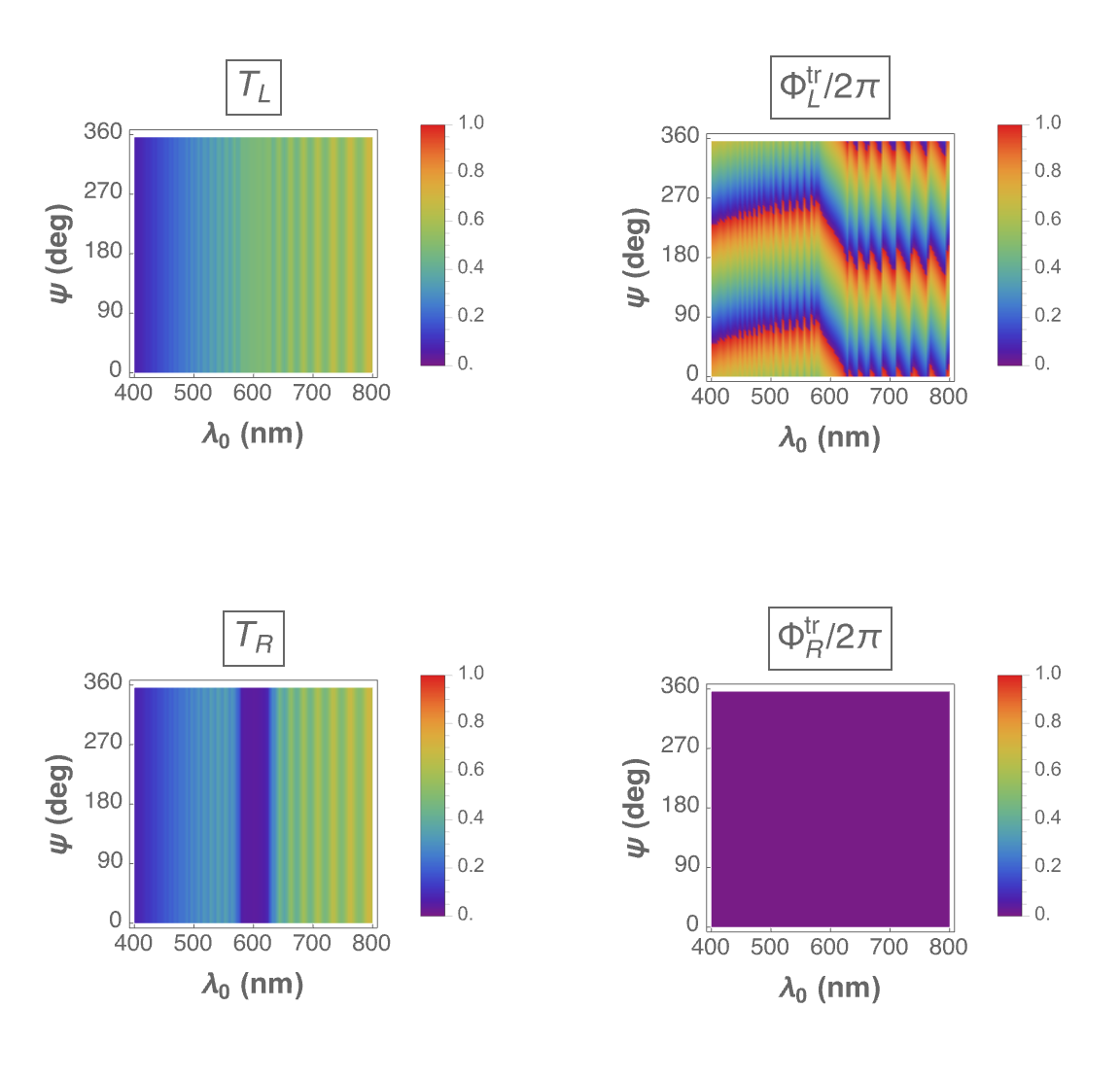
(b) $h=1$, $\theta_{\rm inc}=0^{\circ}$, and $\psi\in[0^{\circ},360^{\circ})$

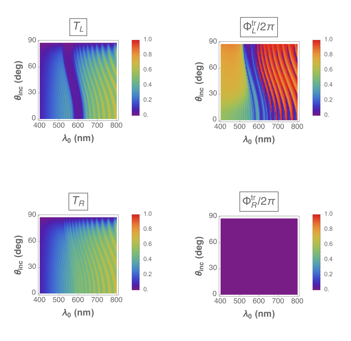
(c) $h=-1$, $\theta_{\rm inc}\in[0^{\circ},90^{\circ})$, and $\psi=0^{\circ}$

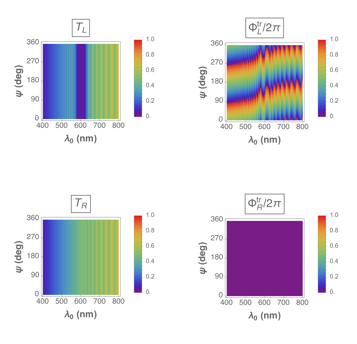
(d) $h=-1$, $\theta_{\rm inc}=0^{\circ}$, and $\psi\in[0^{\circ},360^{\circ})$

Figure 9: Spectral variations of the total circular transmittance $T_{\mu}(\lambda_{\scriptscriptstyle 0},\theta_{\rm inc},\psi)$ and transmission-mode geometric phase $\Phi^{\rm tr}_{\mu}(\lambda_{\scriptscriptstyle 0},\theta_{\rm inc},\psi)$, $\mu\in\left\{L,R\right\}$, when (a,b) $h=1$ and (c,d) $h=-1$. (a,c) $\theta_{\rm inc}\in[0^{\circ},90^{\circ})$ and $\psi=0^{\circ}$; (b,d) $\theta_{\rm inc}=0^{\circ}$ and $\psi\in[0^{\circ},360^{\circ})$.

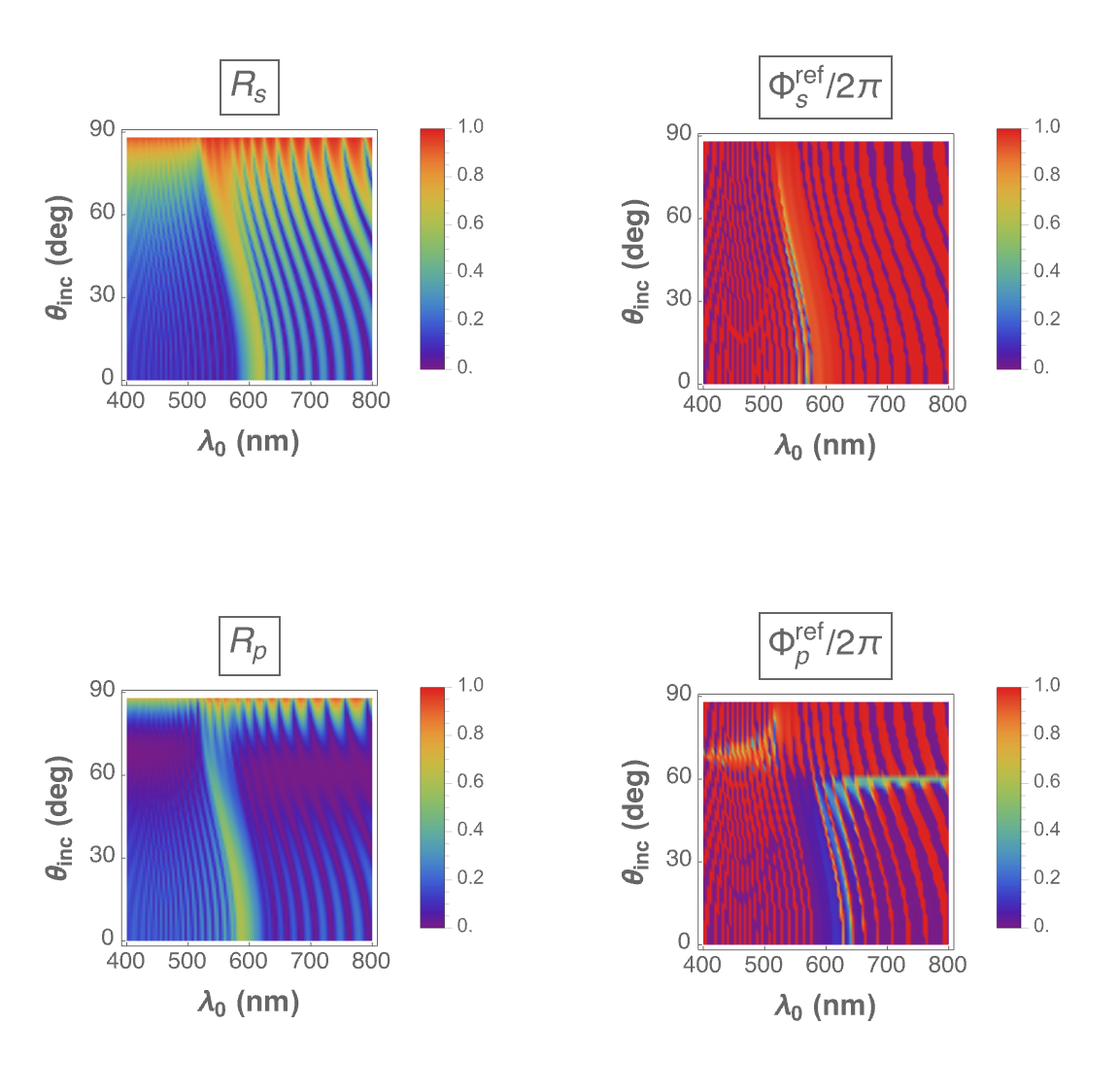
(a) $h=1$, $\theta_{\rm inc}\in[0^{\circ},90^{\circ})$, and $\psi=0^{\circ}$

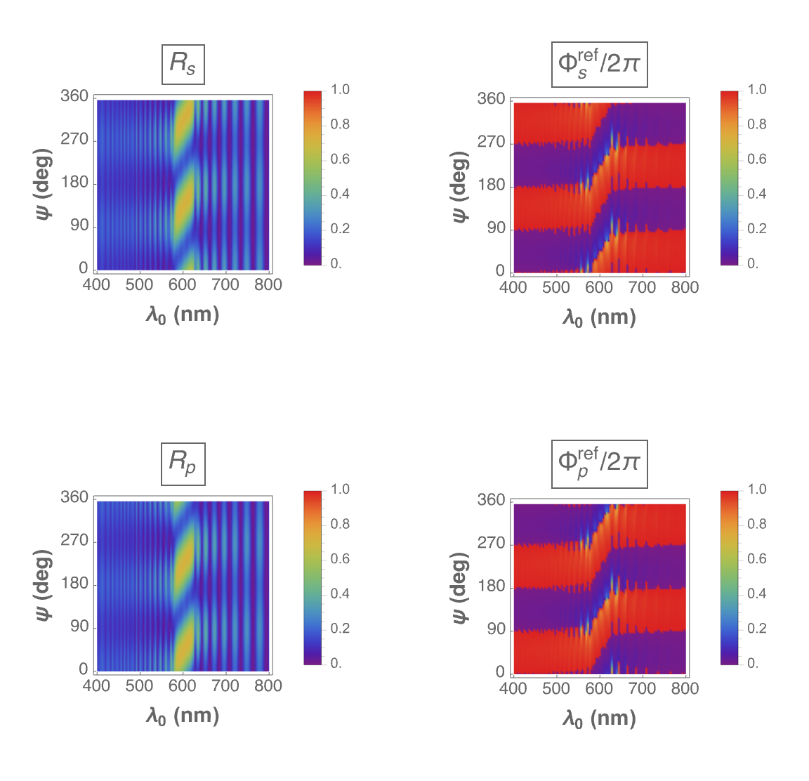
(b) $h=1$, $\theta_{\rm inc}=0^{\circ}$, and $\psi\in[0^{\circ},360^{\circ})$

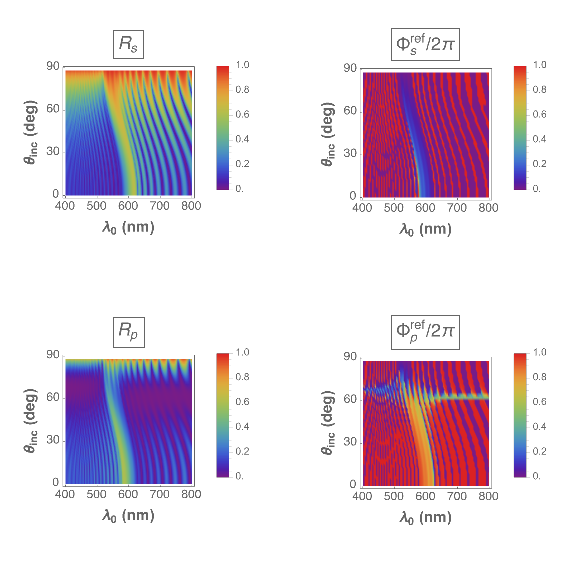
(c) $h=-1$, $\theta_{\rm inc}\in[0^{\circ},90^{\circ})$, and $\psi=0^{\circ}$

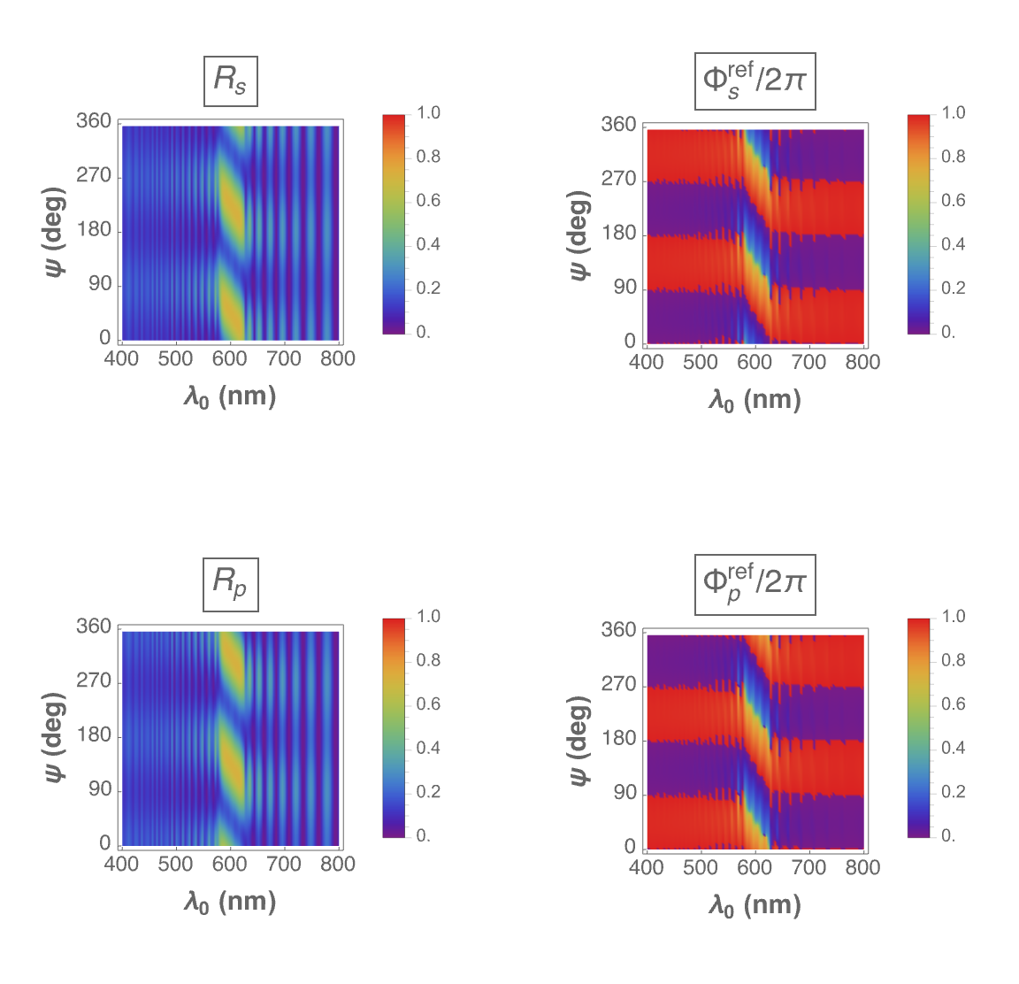
(d) $h=-1$, $\theta_{\rm inc}=0^{\circ}$, and $\psi\in[0^{\circ},360^{\circ})$

Figure 10: Spectral variations of the total linear reflectance $R_{\mu}(\lambda_{\scriptscriptstyle 0},\theta_{\rm inc},\psi)$ and reflection-mode geometric phase $\Phi^{\rm ref}_{\mu}(\lambda_{\scriptscriptstyle 0},\theta_{\rm inc},\psi)$, $\mu\in\left\{s,p\right\}$, when (a,b) $h=1$ and (c,d) $h=-1$. (a,c) $\theta_{\rm inc}\in[0^{\circ},90^{\circ})$ and $\psi=0^{\circ}$; (b,d) $\theta_{\rm inc}=0^{\circ}$ and $\psi\in[0^{\circ},360^{\circ})$.

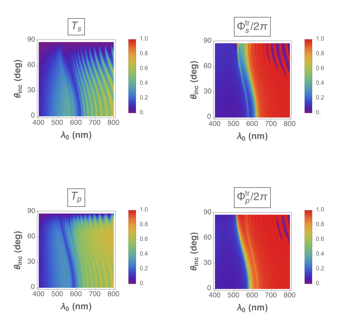
(a) $h=1$, $\theta_{\rm inc}\in[0^{\circ},90^{\circ})$, and $\psi=0^{\circ}$

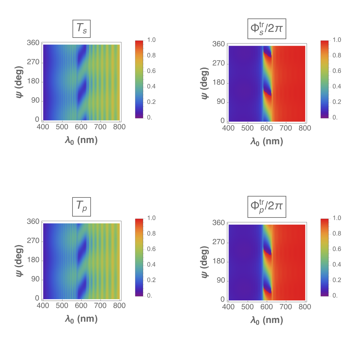
(b) $h=1$, $\theta_{\rm inc}=0^{\circ}$, and $\psi\in[0^{\circ},360^{\circ})$

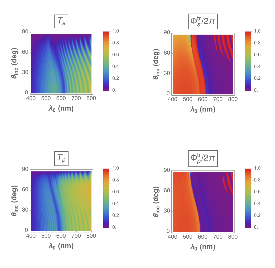
(c) $h=-1$, $\theta_{\rm inc}\in[0^{\circ},90^{\circ})$, and $\psi=0^{\circ}$

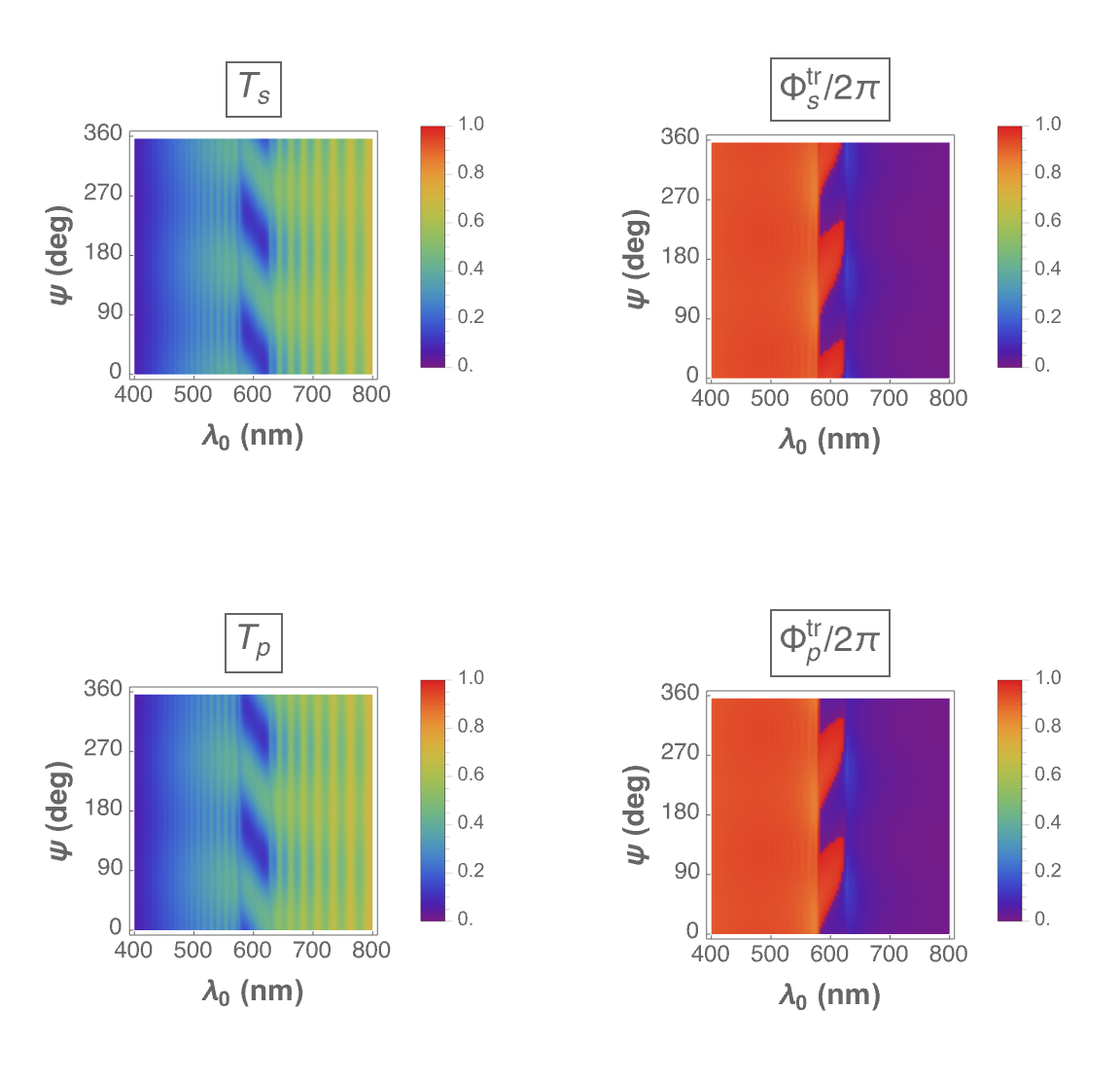
(d) $h=-1$, $\theta_{\rm inc}=0^{\circ}$, and $\psi\in[0^{\circ},360^{\circ})$

Figure 11: Spectral variations of the total linear transmittance $T_{\mu}(\lambda_{\scriptscriptstyle 0},\theta_{\rm inc},\psi)$ and transmission-mode geometric phase $\Phi^{\rm tr}_{\mu}(\lambda_{\scriptscriptstyle 0},\theta_{\rm inc},\psi)$, $\mu\in\left\{s,p\right\}$, when (a,b) $h=1$ and (c,d) $h=-1$. (a,c) $\theta_{\rm inc}\in[0^{\circ},90^{\circ})$ and $\psi=0^{\circ}$; (b,d) $\theta_{\rm inc}=0^{\circ}$ and $\psi\in[0^{\circ},360^{\circ})$.

5 Final remark

Measurement of intensity-dependent observable quantities such as reflectances and transmittances was instrumental in the identification of the circular Bragg phenomenon [43, 45] and continues to be undertaken [12, 11, 20]. However, measurement of phase-dependent quantities, especially for oblique incidence, has been identified in this update as an arena for comprehensive research in the near future.

Appendix: Poincaré spinor and geometric phase

Any uniform plane wave propagating in free space can be represented as a point on the surface of the Poincaré sphere $s_{1}^{2}+s_{2}^{2}+s_{3}^{2}=s_{0}^{2}$, where $s_{0}$, $s_{1}$, $s_{2}$, and $s_{3}$ are the four Stokes parameters. The plane wave’s location is identified by the longitude $\alpha\in[0,2\pi)$ and the latitude $\beta\in[-\pi/2,\pi/2]$ defined through the relations

$$\left.\begin{array}[]{l}s_{1}=s_{0}\,\cos\beta\,\cos\alpha\\[5.0pt] s_{2}=s_{0}\,\cos\beta\,\sin\alpha\\[5.0pt] s_{3}=s_{0}\,\sin\beta\end{array}\right\}\,.$$ (26)

The angles $\alpha$ and $\beta$ appear in the Poincaré spinor

$$\left[{\underline{\phi}}\right]=\left[\begin{array}[]{c}\cos\left(\frac{\pi}{4}-\frac{\beta}{2}\right)\\[5.0pt] \sin\left(\frac{\pi}{4}-\frac{\beta}{2}\right)\exp\left(i\alpha\right)\end{array}\right]\,.$$ (27)

With respect to a plane wave labeled “1”, the geometric phase of a plane wave labeled “2” is defined as the angle

$$\Phi_{21}={\rm Arg}\left\{{\left[{\underline{\phi}}_{1}\right]}^{\dagger}\cdot{\left[{\underline{\phi}}_{2}\right]}\right\}\,.$$ (28)

References

- [1] Faryad, M., Lakhtakia, A.: The circular Bragg phenomenon. Advances in Optics and Photonics 6, 225–292 (2014).
- [2] Lakhtakia, A., Venugopal, V.C.: On Bragg reflection by helicoidal bianisotropic mediums. Archiv für Elektronik und Übertragungstechnik 53, 287–290 (1999).
- [3] Chandrasekhar, S.: Liquid Crystals, 2nd edn. Cambridge University Press, Cambridge, United Kingdom (1993).
- [4] De Gennes, P. G., Prost, J. A.: The Physics of Liquid Crystals, 2nd edn. Oxford University Press, Oxford, United Kingdom (1993).
- [5] Nityananda, R.: On the theory of light propagation in cholesteric liquid crystals. Molecular Crystals and Liquid Crystals 21, 315–331 (1973).
- [6] Parodi, O.: Light propagation along the helical axis in chiral smectics C,” Journal de Physique Colloques 36, C1-325–C1-326 (1975).
- [7] Garoff, S., Meyer, R.B., Barakat, R.: Kinematic and dynamic light scattering from the periodic structure of a chiral smectic liquid crystal. Journal of the Optical Society of America 68, 1217–1225 (1978).
- [8] Abdulhalim, I., Benguigui, L., Weil, R.: Selective reflection by helicoidal liquid crystals. Results of an exact calculation using the 44 characteristic matrix method. Journal de Physique (Paris) 46, 815–825 (1985).
- [9] Xiang, J., Li, Y., Li, Q., Paterson, D.A., Storey, J.M.D., Imrie, C.T., Lavrentovich, O.D.: Electrically tunable selective reflection of light from ultraviolet to visible and infrared by heliconical cholesterics. Advanced Materials 27, 3014–3018 (2015).
- [10] Lakhtakia, A., Messier, R.: Sculptured Thin Films: Nanoengineered Morphology and Optics. SPIE, Bellingham, WA, USA (2005); Chap. 9.
- [11] McAtee, P.D., Lakhtakia, A.: Experimental and theoretical investigation of the co-occurrence of linear and circular dichroisms for oblique incidence of light on chiral sculptured thin films. Journal of the Optical Society of America A 35, 1131–1139 (2018). Replace “” by “” in Eq. (8b).
- [12] Erten, S., Lakhtakia, A., Barber, G.D.: Experimental investigation of circular Bragg phenomenon for oblique incidence. Journal of the Optical Society of America A 32, 764–770 (2015).
- [13] Lakhtakia, A., Weiglhofer, W.S.: Axial propagation in a magnetic-dielectric cholesteric medium. Liquid Crystals 15, 659–667 (1993).
- [14] Lakhtakia, A., Weiglhofer, W.S.: Axial propagation in general helicoidal bianisotropic media. Microwave and Optical Technology Letters 6, 804–806 (1993).
- [15] St. John, W.D., Fritz, W.J., Lu, Z.J., Yang, D.-K.: Bragg reflection from cholesteric liquid crystals. Physical Review E 51, 1191–1198 (1995).
- [16] Lakhtakia, A.: Reflection of an obliquely incident plane wave by a half space filled by a helicoidal bianisotropic medium. Physics Letters A 374, 3887–3894 (2010).
- [17] Lakhtakia, A.: Resilience of circular-polarization-state-sensitive reflection against morphological disorder in chiral structures. Journal of Nanophotonics 18, xxxxxx (2024).
- [18] Wang, F., Lakhtakia, A., Messier, R.: Coupling of Rayleigh–Wood anomalies and the circular Bragg phenomenon in slanted chiral sculptured thin films. European Physics Journal Applied Physics 20, 91–103 (2002).
- [19] Yin, K., Zhan, T., Xiong, J., He, Z., Wu, S.-T.: Polarization volume gratings for near-eye displays and novel photonic devices. Crystals 10, 561 (2020).
- [20] Fiallo, R.A.: Architecting One-dimensional and Three-dimensional Columnar Morphologies of Chiral Sculptured Thin Films, Doctoral Thesis, Pennsylvania State University (2024).
- [21] Das, A., Mandal, S., Fiallo, R.A., Horn, M.W., Lakhtakia, A., Pradhan, M.: Geometric phase and photonic spin Hall effect in thin films with architected columnar morphology. Journal of the Optical Society of America B 40, 2418–2428 (2023). Replace “” by “” in Eq. (5b).
- [22] Lakhtakia, A.: Transmission-mode geometric-phase signatures of circular Bragg phenomenon. Journal of the Optical Society of America B 41, 500–507 (2024).
- [23] Lakhtakia, A.: Geometric phase in plane-wave transmission by a dielectric structurally chiral slab with a central phase defect. Physical Review A 109, 053517 (2024).
- [24] Chen, H.C.: Theory of Electromagnetic Waves: A Coordinate-free Approach. TechBooks, Fairfax, VA, USA (1992).
- [25] Nye, J.F.: Physical Properties of Crystals: Their Representation by Tensors and Matrices. Oxford University Press, Oxford, United Kingdom (1985).
- [26] Dreher, R., Meier, G.: Optical properties of cholesteric liquid crystals. Physical Review A 8, 1616–1623 (1973).
- [27] Sugita, A., Takezoe, H., Ouchi, Y., Fukuda, A., Kuze, E., Goto, N.: Numerical calculation of optical eigenmodes in cholesteric liquid crystals by 44 matrix method. Japanese Journal of Applied Physics 21, 1543–1546 (1982).
- [28] Oldano, C. Miraldi, E., Taverna Valabrega, P.: Dispersion relation for propagation of light in cholesteric liquid crystals. Physical Review A 27, 3291–3299 (1983).
- [29] Lakhtakia, A., Weiglhofer, W.S.: Further results on light propagation in helicoidal bianisotropic mediums: oblique propagation. Proceedings of the Royal Society of London A 453, 93–105 (1997).
- [30] Mackay, T.G., Lakhtakia, A.: The Transfer-Matrix Method in Electromagnetics and Optics. Morgan & Claypool, San Ramon, CA, USA (2020).
- [31] Wooten, F.: Optical Properties of Solids. Academic Press, New York, NY, USA (1972); Sec. 3.1.
- [32] Frisch, M.: ‘The most sacred tenet’? Causal reasoning in physics. British Journal for the Philosophy of Science 60, 459–474 (2009).
- [33] Silva, H., Gross, B.: Some measurements on the validity of the principle of superposition in solid dielectrics. Physical Review 60, 684–687 (1941).
- [34] Kinsler, P.: How to be causal: time, spacetime and spectra. European Journal of Physics 32, 1687–1700 (2011).
- [35] Bragg, W.H., Bragg, W.L.: The reflection of X-rays by crystals. Proceedings of the Royal Society of London A 88, 428–438 (1913).
- [36] Bragg, W.H.: The reflection of X-rays by crystals. Nature 91, 477 (1913).
- [37] Ewald, P.P.: Zur Begründung der Kristalloptik; Teil II: Theorie der Reflexion und Brechung. Annalen der Physik Series 4 49, 117–143 (1916).
- [38] Geddes III, J.B., Meredith, M.W., Lakhtakia, A.: Circular Bragg phenomenon and pulse bleeding in cholesteric liquid crystals. Optics Communications 182, 45–57 (2000).
- [39] Meredith, M.W., Lakhtakia, A.: Time-domain signature of an axially excited cholesteric liquid crystal. Part I: Narrow-extent pulses. Optik 111, 443–453 (2000).
- [40] Geddes III, J.B., Lakhtakia, A.: Time-domain signature of an axially excited cholesteric liquid crystal. Part II: Rectangular wide-extent pulses. Optik 112, 62–66 (2000).
- [41] Born, M., Wolf, E.: Principles of Optics, 6th edn. Cambridge University Press, Cambridge, United Kingdom (1980); Sec. 1.4.2.
- [42] Reusch, E.: Untersuchung über Glimmercombinationen. Annalen der Physik und Chemie (Leipzig) 138, 628–638 (1869).
- [43] Mathieu, J.-P.: Examen de quelques propriétés optiques fondamentales des substances cholestériques. Bulletin de la Société Française de Minéralogie 41, 174–195 (1938).
- [44] Jackson, J.D.: Classical Electrodynamics, 3rd edn. Wiley, New York, NY, USA (1999); Sec. 7.2.
- [45] Fergason, J.L.: Cholesteric structure—I Optical properties. Molecular Crystals 1, 293–307 (1966).