\newsiamremark

remarkRemark \newsiamremarkhypothesisHypothesis \newsiamthmclaimClaim

Random ordinate method for mitigating the ray effect in radiative transport equation simulations

Lei Li School of Mathematical Sciences, Institute of Natural Sciences, MOE-LSC, Shanghai Jiao Tong University, Shanghai, P.R. China. ( ). leili2010@sjtu.edu.cn    Min Tang School of Mathematical Sciences,, Institute of Natural Sciences and MOE-LSC, Shanghai Jiao Tong University, Shanghai, P.R. China. (). tangmin@sjtu.edu.cn    Yuqi Yang School of Mathematical Sciences,, Institute of Natural Sciences, Shanghai Jiao Tong University, Shanghai, P.R. China. (). yangyq1@sjtu.edu.cn
Abstract

The Discrete Ordinates Method (DOM) is the most widely used velocity discretization method for simulating the radiative transport equation. The ray effect stands as a long-standing drawback of DOM. In benchmark tests displaying the ray effect, we observe low regularity in velocity within the solution. To address this issue, we propose a random ordinate method (ROM) to mitigate the ray effect. Compared with other strategies proposed in the literature for mitigating the ray effect, ROM offers several advantages: 1) the computational cost is comparable to DOM; 2) it is simple and requires minimal changes to existing code based on DOM; 3) it is easily parallelizable and independent of the problem setup. Analytical results are presented for the convergence orders of the error and bias, and numerical tests demonstrate its effectiveness in mitigating the ray effect.

keywords:
Random ordinate method, ray effect, discrete ordinate method, radiative transport equation.
{MSCcodes}

1 Introduction

The radiative transport equation (RTE) stands as a fundamental equation governing the evolution of angular flux as particles traverse through a material medium. It provides a statistical description of the density distribution of particles. The RTE has found extensive applications across diverse fields, including astrophysics [22, 26], fusion [25, 23], biomedical optics [16, 7], and biology, among others.

The steady state RTE with anisotropic scattering reads

(1.1) $$\boldsymbol{u}\cdot\nabla\psi(\boldsymbol{z},\boldsymbol{u})+\sigma_{T}(\boldsymbol{z})\psi(\boldsymbol{z},\boldsymbol{u})=\sigma_{S}(\boldsymbol{z})\frac{1}{|S|}\int_{S}P(\boldsymbol{u^{\prime}},\boldsymbol{u})\psi(\boldsymbol{z},\boldsymbol{u^{\prime}})\mathrm{d}\boldsymbol{u^{\prime}}+q(\boldsymbol{z}),$$

subject to the following inflow boundary conditions:

(1.2) $$\psi(\boldsymbol{z},\boldsymbol{u})=\psi_{\Gamma}^{-}(\boldsymbol{z},\boldsymbol{u}),\quad\boldsymbol{z}\in\Gamma^{-}=\partial\Omega,\quad\boldsymbol{u}\cdot\boldsymbol{n}_{\boldsymbol{z}}<0.$$

Here, $\boldsymbol{z}\in\Omega\subset\mathbb{R}^{3}$ represents the spatial variable; $\boldsymbol{u}$ denotes the direction of particle movement, and $S=\{\boldsymbol{u}\mid\boldsymbol{u}\in\mathbb{R}^{3},|\boldsymbol{u}|=1\}$; $\boldsymbol{n}_{\boldsymbol{z}}$ stands for the outward normal vector at position $\boldsymbol{z}$. $\psi(\boldsymbol{z},\boldsymbol{u})$ gives the density of particles moving in the direction $\boldsymbol{u}$ at position $\boldsymbol{z}$. The coefficients $\sigma_{T}(\boldsymbol{z})$, $\sigma_{S}(\boldsymbol{z})$, and $q(\boldsymbol{z})$ represent the total, scattering cross-sections, and the source term, respectively. For physically meaningful situations, $\sigma_{T}(\boldsymbol{z})>\sigma_{S}(\boldsymbol{z})$, for $\forall\boldsymbol{z}\in\Omega$. The kernel $k(\boldsymbol{u}^{\prime},\boldsymbol{u}):=\frac{1}{|S|}P(\boldsymbol{u}^{\prime},\boldsymbol{u})$ is the scattering kernel, which provides the probability that particles moving in the direction $\boldsymbol{u^{\prime}}$ scatter to the direction $\boldsymbol{u}$. For the notational convenience, we will use the symbol $\fint_{S}:=\frac{1}{|S|}\int_{S}$ to denote the average over the domain $S$ associated with the indicated measure. Then, the scaled scattering kernel satisfies:

$$P(\boldsymbol{u}^{\prime},\boldsymbol{u})=P(\boldsymbol{u},\boldsymbol{u^{\prime}}),\qquad\fint_{S}P(\boldsymbol{u^{\prime}},\boldsymbol{u})\mathrm{d}\boldsymbol{u}=\frac{1}{|S|}\int_{S}P(\boldsymbol{u^{\prime}},\boldsymbol{u})\mathrm{d}\boldsymbol{u}=1.$$

The numerical methods for solving the RTE are mainly divided into two categories: particle methods and PDE-based methods. Particle methods, specifically Monte Carlo (MC) methods, simulate the trajectories of numerous particles and collect the density distribution of all particles in the phase space to obtain the RTE solution. The MC methods are known to be slow and noisy but are easy to parallelize and suitable for all geometries [10, 3]. Meanwhile, the PDE-based methods are more accurate and can be faster, but they are not as flexible as the MC method for parallel computation and complex geometries [21]. In this paper, we are interested in the PDE-based method.

The Discrete Ordinates Method (DOM) [2, 6] is the most popular velocity discretization method. DOM approximates the solution to (1.2) using a set of discrete velocity directions $\boldsymbol{u_{m}}$, which are referred to as ordinates. The integral term on the right-hand side of Equation (1.1) is represented by weighted summations of the discrete velocities. DOM retains the positive angular flux and facilitates the determination of boundary conditions. However, solving the RTE using the standard DOM is expensive due to its high dimensionality since the RTE has three spatial variables and two velocity direction variables.

In real applications, people are usually interested in the spatial distributions of some macroscopic quantities, such as the particle density $\int_{S}\psi(\boldsymbol{z},\boldsymbol{u})\mathrm{d}\boldsymbol{u}$, the momentum $\int_{S}\boldsymbol{u}\psi(\boldsymbol{z},\boldsymbol{u})\mathrm{d}\boldsymbol{u}$, etc. Thus, the spatial resolution must be adequate. The computational costs can be significantly reduced if one can obtain the right macroscopic quantities by using a small number of ordinates in DOM.

One natural question arises: Can we improve the accuracy of macroscopic quantities without increasing the number of ordinates? Considerable effort has been invested in discovering a quadrature set with high-order convergence. For the 1D velocity in slab geometry, Gaussian quadrature exists, exhibiting spectral convergence when the solution maintains sufficient smoothness in velocity. However, devising a spectrally convergent 2 or 3-dimensional Gaussian quadrature remains unclear. Furthermore, in section 2, we highlight, through numerical tests, that the solution’s regularity in the velocity direction can be considerably low in some benchmark tests. Consequently, it remains uncertain whether better approximations can be expected, even if a 2 or 3-dimensional Gaussian quadrature with high convergence order for smooth solutions is identified.

When employing a limited number of ordinates in DOM, the ray effect becomes noticeable in numerous 2D spatial benchmark tests [11, 19]. The macroscopic particle density exhibits nonphysical oscillations along the ray paths, particularly noticeable when the inflow boundary conditions or radiation sources demonstrate strong spatial variations or discontinuities. The ray effect stems from particles being confined to move in a limited number of directions. As highlighted in section 2, in benchmark tests displaying the ray effect, we observe low regularity in velocity within the solution, indicating a low convergence order for DOM. In order to mitigate the ray effect, one has to increase the number of ordinates [27], which will significantly increase the computational cost.

The ray effect stands as a long-standing drawback in DOM simulations, and several strategies have been proposed to mitigate these ray effects at reasonable costs. Examples include approaches discussed in [4, 24, 28, 33]. The main idea is to use biased or rotated quadratures or combine the spectral method with DOM. In this paper, inspired by the randomized integration method [29], we introduce a random ordinate method (ROM) for solving RTE. Compared with other ray effect mitigating strategies proposed in the literature, the advantages of ROM are: 1) the computational cost is comparable to DOM; 2) it is simple and makes almost no change to all previous code based on DOM; 3) It is easy to parallelize and independent of the problem setup.

Randomized algorithms can achieve higher convergence order when the solution regularity is low [29]. The concept of the randomized method is straightforward: when approximating $\int_{0}^{1}f(x)dx$, the integral interval $[0,1]$ is partitioned into cells with a maximum size of $h$. Subsequently, an $x_{m}$ is chosen from each interval, and $\int_{0}^{1}f(x)dx$ is approximated by $\sum_{\ell=1}^{n}\omega_{\ell}f(x_{\ell})$, where $\omega_{\ell}$ represents the quadrature weights. With a fixed set of $\{x_{\ell},\omega_{\ell}\}$, one can expect uniform first-order convergence for general $f(x)$ that is Lipschitz continuous. On the other hand, when one randomly chooses a point $x_{\ell}$ inside each interval and keeps using the same $\omega_{\ell}$, the expected error can achieve $O(h^{\frac{3}{2}})$ convergence, whereas the expectation of all randomly chosen quadrature provides $O(h^{3})$ convergence. Randomized algorithms have been developed and analyzed for simple problems, such as the initial value problem of ordinary differential equation (ODE) systems [32, 31], whose complexity has been studied in [13, 9], and for stochastic differential equations [8], whose complexity is analyzed in [5].

The main idea of ROM is that the velocity space is partitioned into $n$ cells, and a random ordinate is selected from each cell. A DOM system with those randomly chosen ordinates is then solved. The ROM solutions’ expected values can achieve a higher convergence order in velocity space. Both theoretical and numerical results indicate that, even with carefully chosen quadratures in DOM, it can only achieve a similar convergence order as ROM when the solution regularity is low. Consequently, the accuracy doesn’t decrease for a single run. However, averaging multiple runs can lead to a higher-order convergence and mitigate the ray effect. Since different runs employ distinct ordinates, ROM allows for easy parallel computation. Therefore, one can mitigate the ray effect by running a lot of samples with a few ordinates and then calculating their expectation.

This paper is structured as follows: Section 2 delves into the ray effects of DOM and illustrates the low regularity of the solution in velocity space. Details of the ROM are described in Section 3. In Section 4, analytical results are presented for the convergence orders of the error and bias when ROM is applied to RTE with isotropic scattering in slab geometry. Section 5 displays the numerical performance of the ROM, demonstrating its ability to mitigate the ray effect. Finally, Section 6 concludes the paper with discussions.

2 Ray effects and low regularity

2.1 Discrete Ordinate Method and Ray Effects

The DOM is the most popular angular discretization for RTE simulations, it writes [18]:

$$\boldsymbol{u}_{\ell}\cdot\nabla\psi_{\ell}(\boldsymbol{z})+\sigma_{T}(\boldsymbol{z})\psi_{\ell}(\boldsymbol{z})=\sigma_{S}(\boldsymbol{z})\sum_{\ell^{\prime}\in V}w_{\ell^{\prime}}P_{\ell,\ell^{\prime}}\psi_{\ell^{\prime}}(\boldsymbol{z})+q_{\ell}(\boldsymbol{z}),\quad\ell\in V,$$

subject to the following inflow boundary conditions:

$$\psi(\boldsymbol{z},\boldsymbol{u}_{\ell})=\psi_{\ell}^{-}(\boldsymbol{z},\boldsymbol{u}),\quad\boldsymbol{z}\in\Gamma^{-}=\partial\Omega,\quad\boldsymbol{u}_{\ell}\cdot\boldsymbol{n}_{\boldsymbol{z}}<0.$$

where $\omega_{\ell}$ is the weight of the quadrature node $\boldsymbol{u}_{\ell}$, satisfying $\sum_{\ell\in V}\omega_{\ell}=1$; $V$ represents the index set of the quadrature $\{\boldsymbol{u}_{\ell},\omega_{\ell}\}$; $P_{\ell,\ell^{\prime}}\approx P(\boldsymbol{u_{\ell}},\boldsymbol{u_{\ell^{\prime}}})$ denotes the discrete scattering kernel; $q_{\ell}(\boldsymbol{z})\approx q\left(\boldsymbol{z},\boldsymbol{u}_{\ell}\right)$. Then $\psi_{\ell}(\boldsymbol{z})\approx\psi\left(\boldsymbol{z},\boldsymbol{u}_{\ell}\right)$ and, for all $\ell\in V$,

$$\sum_{\ell^{\prime}\in V}\omega_{\ell^{\prime}}P_{\ell,\ell^{\prime}}\psi_{\ell^{\prime}}(\boldsymbol{z})\approx\fint_{S}P(\boldsymbol{u_{\ell}},\boldsymbol{u}_{\ell^{\prime}})\psi(\boldsymbol{z},\boldsymbol{u}_{\ell^{\prime}})\mathrm{d}\boldsymbol{u}_{\ell^{\prime}}.$$

In slab geometry, where $S=[-1,1]$ and $\Omega=[x_{L},x_{R}]$, the RTE reads, for $(\mu,x)\in[-1,1]\times[x_{L},x_{R}]$:

$$\mu\partial_{x}{}\psi(x,\mu)+\sigma_{T}(x)\psi(x,\mu)=\sigma_{S}(x)\frac{1}{2}\int_{-1}^{1}P(\mu^{\prime},\mu)\psi(x,\mu^{\prime})d\mu^{\prime}+q(x),$$

subject to the boundary conditions:

(2.1) $$\psi(x_{L},\mu)=\psi_{L}(\mu),\quad\mu>0;\qquad\psi(x_{R},\mu)=\psi_{R}(\mu),\quad\mu<0.$$

The DOM in slab geometry takes $V=\{-M,M+1,\cdots,-1,1,\cdots,M-1,M\}$, where $M$ is an integer. The discrete ordinates $\mu_{\ell}$ ($\ell\in V$) satisfy:

$$0<\mu_{1}<\cdots<\mu_{M-1}<\mu_{M}<1,\qquad\mu_{-\ell}=-\mu_{\ell}.$$

Therefore, the DOM in slab geometry becomes:

(2.2) $$\Big{(}\mu_{\ell}\partial_{x}+\sigma_{T}(x)\Big{)}\psi_{\ell}(x)=\sigma_{S}(x)\sum_{\ell^{\prime}\in V}\omega_{\ell^{\prime}}P_{\ell,\ell^{\prime}}\psi_{\ell}(x)+q_{\ell}(x),$$

subject to the boundary conditions:

$$\psi_{\ell}\left(x_{L}\right)=\psi_{L}\left(\mu_{\ell}\right),\quad\mu_{\ell}>0;\quad\psi_{\ell}\left(x_{R}\right)=\psi_{R}\left(\mu_{\ell}\right),\quad\mu_{\ell}<0.$$

Two commonly used quadratures are the Uniform quadrature and the Gaussian quadrature. For the uniform quadrature, $[-1,1]$ is divided into $2M$ equally spaced cells, each of size $\Delta\mu=1/M$. The values $\{\mu_{\ell}|\ell\in V\}$ represent the midpoint of each cell, i.e., $\mu_{\ell}=\frac{2\ell-1}{2M}$ for $\ell>0$ and $\mu_{\ell}=\frac{2{\ell}+1}{2M}$ for $\ell<0$, while $\omega_{\ell}=1/M$. For the Gaussian quadrature, $\{\mu_{\ell}|\ell\in V\}$ consists of $2M$ distinct roots of Legendre polynomials of degree $2M$ denoted by $L_{2M}(x)$, and the weights $\omega_{\ell}=2/[(1-\mu_{\ell}^{2})(L_{2M}^{\prime}(\mu_{\ell}))^{2}]$.

For RTE in the X-Y geometry, where the 3D velocity on a unit sphere is projected to a 2D disk, suppose that the DOM has $M$ points in each quadrant. Then, the 2D discrete velocity directions defined on a disk are $\mathbf{\boldsymbol{u}_{\ell}}=(c_{\ell},s_{\ell})$ for ${\ell}\in\bar{V}=\{1,2,\cdots M,\cdots,4M\}$ when $M$ is an integer. The DOM in X-Y geometry is expressed as follows, for ${\ell}\in\bar{V}$ and $(x,y)\in[x_{L},x_{R}]\times[y_{B},y_{T}]$:

$$\Big{(}c_{\ell}\partial_{x}+s_{\ell}\partial_{y}+\sigma_{T}(x,y)\Big{)}\psi_{m}(x,y)=\sigma_{S}(x,y)\sum_{\ell^{\prime}\in\bar{V}}\bar{\omega}_{\ell^{\prime}}P_{\ell,\ell^{\prime}}\psi_{\ell^{\prime}}(x,y)+q_{\ell}(x,y),$$

where

$$(c_{\ell},s_{\ell})=\Big{(}\left(1-\zeta_{\ell}^{2}\right)^{\frac{1}{2}}\cos\theta_{\ell},\left(1-\zeta_{\ell}^{2}\right)^{\frac{1}{2}}\sin\theta_{\ell}\Big{)},\quad\mbox{with }\zeta_{\ell}\in(0,1),\theta_{\ell}\in(0,2\pi).$$

The boundary conditions become

$$\left\{\begin{array}[]{llll}\psi_{\ell}\left(x_{L},y\right)=\psi_{L,\ell}(y),&c_{\ell}>0;&\psi_{\ell}\left(x_{R},y\right)=\psi_{R,\ell}(y),&c_{\ell}<0;\\ \psi_{\ell}\left(x,y_{B}\right)=\psi_{B,\ell}(x),&s_{\ell}>0;&\psi_{\ell}\left(x,y_{T}\right)=\psi_{T,\ell}(x),&s_{\ell}<0.\end{array}\right.$$

Two kinds of quadratures discussed in [21] are considered. Each quadrant has $M$ discrete velocities, and we only show the details for the first quadrant such that $\zeta_{\ell}\in(0,1)$ and $\theta_{\ell}\in(0,\frac{\pi}{2})$. The discrete velocities in other quadrants are obtained by symmetry.

The first one is referred to as ”2D uniform quadrature”. Each quadrant has $M=N^{2}$ ordinates, and the nodes are uniform in the $(\zeta,\theta)$ plane. More precisely, $(\zeta_{i},\theta_{j})=(\frac{2N-2i+1}{2N},\frac{2j-1}{4N}\pi)$ for $i=1,\cdots,N$; $j=1,\cdots,N$ and $\bar{\omega}_{\ell}=\frac{1}{4N^{2}}$. Then for $M=N^{2}$ and all $\ell\in\{1,\cdots,M\}$, there exists a pair of integers $(i,j)$ with $i,j\in\{1,\cdots,N\}$ such that $\ell=(i-1)N+j$ and

(2.3) $$(c_{\ell},s_{\ell},\bar{\omega}_{\ell})=\Big{(}\big{(}1-\zeta_{i}^{2}\big{)}^{\frac{1}{2}}\cos\theta_{j},\big{(}1-\zeta_{i}^{2}\big{)}^{\frac{1}{2}}\sin\theta_{j},\frac{1}{4N^{2}}\Big{)}.$$

The second one is the 2D Gaussian quadrature described in [21], for which each quadrant has $M=N(N+1)/2$ ordinates. Each quadrant has $N$ distinct $\zeta_{i}$, $i\in\{1,\cdots,N\}$, which are the $N$ positive roots of $L_{2N}(\zeta)$, the Legendre polynomial of degree $2N$. They are arranged as

$$1>\zeta_{1}>\zeta_{2}>\cdots>\zeta_{N}>0.$$

Each $\zeta_{i}$ corresponds to $N$ distinct $\theta_{i,j}=\frac{2j-1}{4i}\pi,j=1,2,\cdots,i$, and the weight for the velocity direction $(\zeta_{i},\theta_{i,j})$ is uniform in $j$ such that

$$\bar{\omega}_{i}=\frac{1}{2i\left(1-\zeta_{i}^{2}\right)\left[L_{2N}^{\prime}\left(\zeta_{i}\right)\right]^{2}}.$$

Then for $M=N(N+1)/2$ and all $\ell\in\{1,\cdots,M\}$, there exists a pair of integers $(i,j)$ such that $i\in\{1,\cdots,N\}$, $1\leq j\leq i$, and $\ell=\frac{i(i-1)}{2}+j$ and

$$\left(c_{\ell},s_{\ell},\bar{\omega}_{\ell}\right)=\Big{(}\big{(}1-\zeta_{i}^{2}\big{)}^{\frac{1}{2}}\cos\theta_{i,j},\big{(}1-\zeta_{i}^{2}\big{)}^{\frac{1}{2}}\sin\theta_{i,j},\frac{1}{2i\left(1-\zeta_{i}^{2}\right)\left[L_{2N}^{\prime}\left(\zeta_{i}\right)\right]^{2}}\Big{)}.$$

The rest part of the quadrature set can be constructed by symmetry:
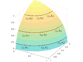
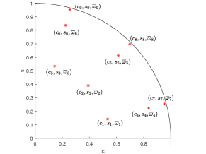
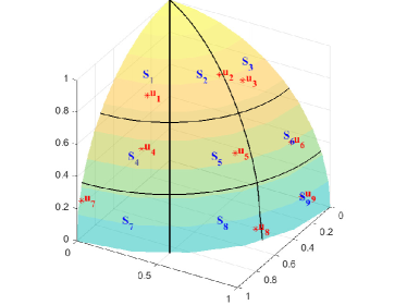
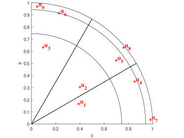
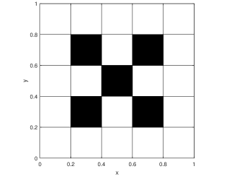
$$\bar{\omega}_{\ell}=\bar{\omega}_{\ell+M}=\bar{\omega}_{\ell+2M}=\bar{\omega}_{\ell+4M},$$
$$\theta_{\ell}=\pi-\theta_{\ell+M}=\theta_{\ell+2M}+\pi=-\theta_{\ell+4M},\qquad\zeta_{\ell}=\zeta_{\ell+M}=\zeta_{\ell+2M}=\zeta_{\ell+4M}.$$

Let’s take $N=3$, the chosen discrete ordinates of Uniform and Gaussian quadratures in one quadrant are plotted in Figure 1. The selected ordinates on the surface of a 3D unit sphere and their corresponding projections to the 2D unit disk are displayed.

Refer to caption
Refer to caption
Refer to caption
Refer to caption
Figure 1: Schematic diagram of selected ordinates on the surface of a 3D unit sphere and their corresponding projection to the 2D unit disk. (a)(b) Uniform quadrature; (c)(d) Gaussian quadrature.

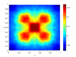
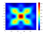
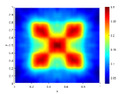
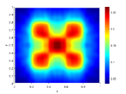
It has long been known that the solution of DOM exhibits the ray effect, especially when there are discontinuous source terms in the computational domain [4, 24, 33]. This phenomenon cannot be improved by increasing the spatial resolution. We show one typical example to demonstrate the ray effects.

Example 2.1.

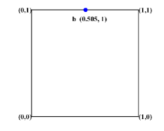
We consider RTE in the X-Y geometry with a localized source term at the center of the computational domain. Let

$$x\times y\in\Omega=[0,1]\times[0,1],\quad\sigma_{T}=1,\quad\sigma_{S}=0.5.$$
$$q(x,y)=\left\{\begin{aligned} 2,&\quad(x,y)\in[0.4,0.6]\times[0.4,0.6],\\ 0,&\quad\mbox{elsewhere}.\\ \end{aligned}\right.$$

The inflow boundary conditions are zero.

We consider the isotropic and anisotropic scattering with the following scattering kernel

(2.4) $$P(\boldsymbol{u},\boldsymbol{u^{\prime}})=G(\boldsymbol{u}\cdot\boldsymbol{u^{\prime}})=G(\cos\xi)=1+g\cdot\cos\xi,$$

where $\xi$ is the included angle between $\boldsymbol{u}$ and $\boldsymbol{u^{\prime}}$. When $g=0$, (2.4) gives isotropic scattering, meaning particles moving with velocity $\boldsymbol{u}$ will scatter into a new velocity $\boldsymbol{u}^{\prime}$ with uniform probability for all $\boldsymbol{u}^{\prime}$. When $g=0.9$, (2.4) gives anisotropic scattering, implying that when the included angle $\xi$ between $\boldsymbol{u}$ and $\boldsymbol{u^{\prime}}$ is smaller, the probability that particles moving with velocity $\boldsymbol{u}$ scatter into $\boldsymbol{u}^{\prime}$ is higher.

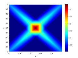
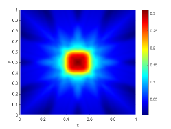
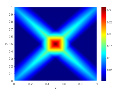
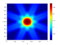
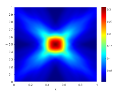
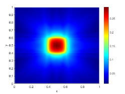
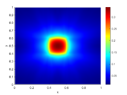
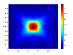
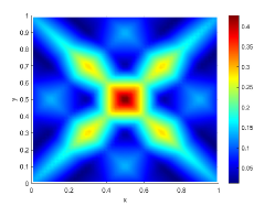
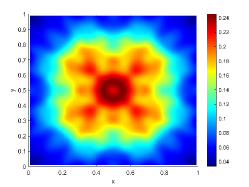
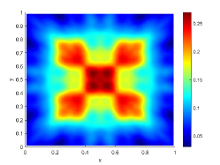
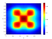
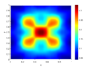
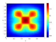
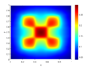
The computational domain is partitioned into $100\times 100$ spatial cells. We employ Uniform quadrature sets with various numbers of ordinates. The numerical results of the average density $\phi(x,y)=\sum_{\ell\in V}\bar{\omega}_{\ell}\psi_{\ell}(x,y)$ are displayed in Figure 2. From left to right, $4$, $16$, and $36$ ordinates of Uniform quadrature as in (2.3) are used. We can observe that the solutions exhibit rays that correspond to the chosen ordinates of the DOM. The solutions have poor accuracy, violate the rotational invariance property, and this phenomenon does not disappear with the refinement of the spatial grids.

Refer to caption
(a) 4 ordinates
Refer to caption
(b) 16 ordinates
Refer to caption
(c) 36 ordinates
Refer to caption
(d) 4 ordinates
Refer to caption
(e) 16 ordinates
Refer to caption
(f) 36 ordinates
Figure 2: Demonstration of the ray effects. The average densities $\phi(x,y)$ calculated with different numbers of ordinates are displayed. The numerical results are calculated with $100\times 100$ spatial cells and uniform quadrature. (a)(b)(c): isotropic scattering kernel with $g=0$ in (2.4); (d)(e)(f) anisotropic scattering kernel with $g=0.9$ in (2.4).

2.2 Low regularity and Convergence order

In this subsection, we first demonstrate numerically that for the tests that exhibit ray effects, the solutions usually have a low regularity in velocity space. The 2D solution has sharp transition in velocity space and the positions of the transitional points are spatially dependent. No matter what quadrature sets are chosen, high order convergence can only be achieved for smooth functions. Therefore, it is difficult to improve the solution accuracy without increasing the quadrature nodes when the regularity is low. Then, we show numerically, in both slab and X-Y geometries, that the convergence order of DOM decreases as the solution regularity in the velocity space decreases.

2.2.1 The slab geometry case

We solve equation (2.2) and test both the Uniform and Gaussian quadratures. We employ second-order finite difference spatial discretization in [14] to obtain the numerical results. The number of spatial cells is fixed to be $I=50$, and the grid points are $x_{i}$ ($i=0,1,\cdots,I$). Let $\psi_{\ell}(x_{i})$ be the solution to (2.2), and the average density $\phi(x_{i})=\sum_{{\ell}\in V}\omega_{\ell}\psi_{\ell}(x_{i})$. The reference solution is computed using $1280$ ordinates. The $\ell^{2}$ errors of the numerical solutions with different ordinates are defined by

$$\mathcal{E}=\sqrt{\frac{1}{I+1}\sum_{i=0}^{I}\mid\phi(x_{i})-\phi^{ref}(x_{i})\mid^{2}}.$$

Though there is no ray effect in slab geometry, we will show in the following example that when the inflow boundary conditions have low regularity in velocity space, the convergence orders of DOM are low.

Example 2.2.

Let the computational domain, total and absorption cross sections, scattering kernel and source term be respectively

$$x\in[0,1],\quad\sigma_{T}(x)=10x^{2}+1,\quad\sigma_{S}(x)=5x^{2}+0.5,\quad P(\mu^{\prime},\mu)=1,\quad q(x)=1+x.$$

We consider three different inflow boundary conditions:

  1. Case 1:

    Continuous and smooth inflow boundary conditions:

    (2.5) $$\psi(0,\mu)=3\mu,\quad\mu>0;\qquad\psi(1,\mu)=-5\mu,\quad\mu<0.$$
  2. Case 2:

    Continuous but non-differentiable inflow boundary conditions:

    (2.6) $$\psi(0,\mu)=\begin{cases}\frac{4}{3}-\mu,&\frac{1}{3}<\mu<1,\\ 3\mu,&0<\mu\leq\frac{1}{3},\end{cases}\qquad\psi(1,\mu)=\begin{cases}2+\mu,&-1<\mu<-\frac{1}{3},\\ -5\mu,&-\frac{1}{3}\leq\mu<0.\end{cases}$$
  3. Case 3:

    Discontinuous inflow boundary conditions:

    (2.7) $$\psi(0,\mu)=\begin{cases}3-\mu,&\frac{1}{3}<\mu<1,\\ 3\mu,&0<\mu\leq\frac{1}{3},\end{cases}\qquad\psi(1,\mu)=\begin{cases}4+\mu,&-1<\mu<-\frac{1}{3},\\ -5\mu,&-\frac{1}{3}\leq\mu<0.\end{cases}$$

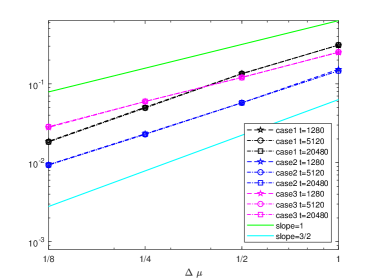
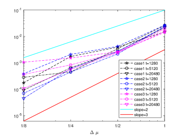
The convergence orders of DOM for different cases are shown in Figure 3. One can observe that for both Uniform and Gaussian quadratures, the convergence orders decrease from 2 to 1 when the inflow boundary conditions change from Case 1 to Case 3. Therefore, one cannot expect a high convergence order when the regularity of the inflow boundary conditions is low. In particular, Gaussian quadrature does not reach spectral convergence as shown in Figure 3(b). This is because, though the inflow boundary condition is smooth in $\mu$, at the boundary, the solution jumps at $\mu=0$. Gaussian quadrature does not provide spectral convergence for solutions with a jump at $\mu=0$.

Refer to caption
(a) Uniform quadrature
Refer to caption
(b) Gaussian quadrature
Figure 3: Example 2.2: Convergence orders of DOM with different inflow boundary conditions in (2.5)-(2.7). (a): Uniform quadratures of different sizes; (b): Gaussian quadratures of different sizes. Here $\Delta\mu=\frac{1}{M}$.

2.2.2 The X-Y geometry case

We solve Example 2.1. The classical second-order diamond difference (DD) method [21] is adopted for the spatial discretization. Since only the convergence order in the velocity variable is considered in this paper, after spatial discretization, the reference solution can be considered as a large integral system for unknowns at the given spatial grids. We use the same spatial mesh and discretizations throughout the paper, eliminating the need to consider the error introduced by the spatial discretization. We would like to emphasize that the main purpose of our current work is to show the convergence orders of the velocity discretization; any spatial discretization can be chosen to obtain the numerical results.

The spatial domain $\Omega=[x_{L},x_{R}]\times[y_{B},y_{T}]$ is divided into $I\times J$ uniform cells. Let $\Delta x=\frac{x_{R}-x_{L}}{I}$, $\Delta y=\frac{y_{T}-y_{B}}{J}$, $x_{0}=x_{L}$, $y_{0}=y_{B}$ and

$$x_{i}=x_{L}+i\Delta x,\quad x_{i+\frac{1}{2}}=x_{L}+\big{(}i-\frac{1}{2}\big{)}\Delta x,\quad\mbox{for $i=1,\cdots,I$,}$$
$$y_{j}=y_{B}+j\Delta y,\quad y_{j+\frac{1}{2}}=y_{B}+\big{(}j-\frac{1}{2}\big{)}\Delta y,\quad\mbox{for $j=1,\cdots,J$.}$$

We use DD with $I=100$, $J=100$. The grid points of the two-dimensional DD method are at the cell centers, i.e. approximations of $\psi_{\ell}(x_{i-\frac{1}{2}},y_{j-\frac{1}{2}})$ and the average density $\phi(x_{i-\frac{1}{2}},y_{j-\frac{1}{2}})=\sum_{\ell\in V}\bar{\omega}_{\ell}\psi_{\ell}(x_{i-\frac{1}{2}},y_{j-\frac{1}{2}})$ (for $i=1,\cdots,I$, $j=1,\cdots,J$) are obtained. The $\ell^{2}$ errors between the reference solution $\phi^{ref}$ and the numerical solutions $\phi$ obtained by different quadratures are defined by

(2.8) $$\mathcal{E}=\sqrt{\frac{1}{IJ}\Big{(}\sum_{i=0}^{I-1}\sum_{j=0}^{J-1}\mid\phi(x_{i+\frac{1}{2}},y_{j+\frac{1}{2}})-\phi^{ref}(x_{i+\frac{1}{2}},y_{j+\frac{1}{2}})\mid^{2}\Big{)}}.$$

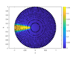
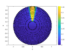
The reference solution of the Uniform (Gaussian) quadrature $\phi_{U}^{ref}$ ($\phi_{G}^{ref}$) is computed by $N=20$, which indicates $1600$ ($840$) ordinates on the 2D disk. As shown in Table 1, the convergence orders of both quadratures are around 0.74. In Figure 4, we plot the velocity distribution of $\psi_{U}^{ref}$ on the $(c,s)$ plane near two midpoints of the left and right boundaries. It can be seen that the solution varies rapidly in the velocity variable.

Table 1: Example 2.1: Convergence orders of DOM with the scattering kernel as in (2.4). Here $\Delta S=\frac{\pi}{4M}$.
$\Delta S$ $\pi/100$ $\pi/64$ $\pi/36$ $\pi/16$ Order
Uniform g=0 4.337E-03 5.560E-03 8.672E-03 1.629E-02 0.73
g=0.9 4.354E-03 5.580E-03 8.707E-03 2.075E-02 0.73
Gaussian g=0 3.966E-03 5.496E-03 8.862E-03 1.477E-02 0.75
g=0.9 3.978E-03 5.518E-03 8.902E-03 1.491E-02 0.75
Refer to caption
(a) point a
Refer to caption
(b) g=0
Refer to caption
(c) g=0.9
Refer to caption
(d) point b
Refer to caption
(e) g=0
Refer to caption
(f) g=0.9
Figure 4: Example 2.1: The velocity distribution of $\psi$ at given spatial positions. a) d) display the locations of two different points $a$ and $b$. b) c) The heat map of $(c_{m},s_{m},\psi_{m}(a))$, $\forall m\in\bar{V}$. e) f) The heat map of $(c_{m},s_{m},\psi_{m}(b))$, $\forall m\in\bar{V}$. The black ${}^{\prime}+^{\prime}$ indicate the locations of all ordinates $(c_{m},s_{m})$.

3 Random ordinate method

The ROM is based on DOM, but the ordinates are chosen randomly. More precisely, the ROM is performed as following:

  1. 1.

    The velocity space $S$ is divided into $n$ cells and each cell is denoted by $S_{\ell}$ ($\ell=1,\cdots,n$). The maximum area of all $S_{\ell}$ is denoted by $\Delta S=\max_{\ell=1,\cdots,n}|S_{\ell}|$. For example in 1D, $S=[-1,1]$, if uniform mesh is employed, then $\Delta S=2/n$.

  2. 2.

    Sample randomly one ordinate from each cell with uniform probability. Denote $\mathbb{V}^{\xi}=\{\boldsymbol{u}_{1},\cdots,\boldsymbol{u}_{n}\}$ as the tuple of random ordinates and $V^{\xi}$ as the index set.

  3. 3.

    Solve the resulting discrete ordinate system with the randomly chosen velocity directions.

    (3.1) $$\boldsymbol{u_{\ell}}\cdot\nabla\psi_{\ell}(\boldsymbol{z})+\sigma_{T}(\boldsymbol{z})\psi_{\ell}(\boldsymbol{z})=\sigma_{S}(\boldsymbol{z})\sum_{\ell^{\prime}=1}^{n}\omega_{\ell^{\prime}}P_{\ell^{\prime},\ell}\psi_{\ell^{\prime}}(\boldsymbol{z})+q_{\ell}(\boldsymbol{z}),\quad\boldsymbol{u_{\ell}}\in\mathbb{V}^{\xi},$$

    subject to the boundary conditions

    (3.2) $$\psi_{\ell}(\boldsymbol{z})=\psi_{\Gamma}^{-}(\boldsymbol{z},\boldsymbol{u_{\ell}}),\quad\boldsymbol{z}\in\Gamma^{-}=\partial\Omega,\quad\boldsymbol{u_{\ell}}\in\mathbb{V}^{\xi},\quad\boldsymbol{u_{\ell}}\cdot\boldsymbol{n}_{\boldsymbol{z}}<0.$$

Since $\boldsymbol{u_{\ell}}$ are now randomly chosen, to guarantee the solution accuracy, one has to determine the corresponding discrete weights $\omega_{\ell}$ and discrete scattering kernel $P_{\ell^{\prime},\ell}$. We will simply choose the following approximation:

(3.3) $$\displaystyle\frac{1}{|S|}\int_{S}P(\boldsymbol{u^{\prime}},\boldsymbol{u}_{\ell})\psi(\boldsymbol{z},\boldsymbol{u^{\prime}})\,d\boldsymbol{u^{\prime}}\approx\sum_{\ell^{\prime}=1}^{n}\omega_{\ell^{\prime}}P_{\ell^{\prime},\ell}\psi_{\ell^{\prime}}(\boldsymbol{z}),$$

where

(3.4) $$\omega_{\ell^{\prime}}=\frac{|S_{\ell^{\prime}}|}{|S|},\qquad P_{\ell^{\prime},\ell}=P(\boldsymbol{u}_{\ell^{\prime}},\boldsymbol{u}_{\ell}).$$

Such a choice clearly satisfies $\sum_{\ell=1}^{n}\omega_{\ell}=1$. If $\ell^{\prime}\neq\ell$, then

$$\mathbb{E}_{\mu_{\ell^{\prime}}}P_{\ell^{\prime},\ell}\psi_{\ell^{\prime}}(\boldsymbol{z})=\frac{1}{|S_{\ell^{\prime}}|}\int_{S_{\ell^{\prime}}}P(\boldsymbol{u}^{\prime},\boldsymbol{u}_{\ell})\psi(\boldsymbol{z},\boldsymbol{u}^{\prime})d\boldsymbol{u}^{\prime}.$$

Therefore, the expectation of the weighted summation provides a good approximation to the integration on the right hand side of (1.1). More precisely,

$\displaystyle\sum_{\ell^{\prime}=1}^{n}\omega_{\ell^{\prime}}\mathbb{E}_{\mu_{\ell^{\prime}}}P_{\ell^{\prime},\ell}\psi_{\ell^{\prime}}(\boldsymbol{z})=$ $\displaystyle\frac{1}{|S|}\int_{S}P(\boldsymbol{u^{\prime}},\boldsymbol{u}_{\ell})\psi(\boldsymbol{z},\boldsymbol{u^{\prime}})\,d\boldsymbol{u^{\prime}}$
$\displaystyle-\frac{|S_{\ell}|}{|S|}\int_{S_{\ell}}P(\boldsymbol{u^{\prime}},\boldsymbol{u}_{\ell})\psi(\boldsymbol{z},\boldsymbol{u^{\prime}})\,d\boldsymbol{u^{\prime}}+\omega_{\ell}P(\boldsymbol{u}_{\ell},\boldsymbol{u}_{\ell})\psi(\boldsymbol{z},\boldsymbol{u}_{\ell})$
$\displaystyle=$ $\displaystyle\frac{1}{|S|}\int_{S}P(\boldsymbol{u^{\prime}},\boldsymbol{u}_{\ell})\psi(\boldsymbol{z},\boldsymbol{u^{\prime}})\,d\boldsymbol{u^{\prime}}+O(|S_{\ell}|^{2}D(S_{\ell})).$

where $D(S_{\ell})$ means the diameter of the $\ell$-th cell. By employing such a straightforward strategy, there exists the possibility that $\sum_{\ell^{\prime}}P_{\ell,\ell^{\prime}}\omega_{\ell^{\prime}}\neq 1$, potentially leading to a violation of mass conservation at the discrete level. Nonetheless, the positivity of the solution is maintained. Since we consider only $O(1)$ total and scattering cross sections in this current work, only a small error is introduced.

According to [6, 17], symmetric ordinates perform better, especially when there are multiscale parameters in the computational domain. Although we do not consider multiscale parameters in this current paper, symmetric ordinates are used in the ROM. More precisely, in slab geometry, let $n=2m$ and $S_{1}\cup S_{2}\cup\cdots\cup S_{m}=[-1,0]$. $\mu_{\ell}$ ($\ell=1,\cdots,m$) are randomly sampled from $S_{\ell}$ with a uniform distribution. Then

$$\mu_{m+\ell}=-\mu_{m+1-\ell},\quad\mbox{for $\ell=1,2,\cdots,m$}.$$

In the X-Y geometry, let $n=4m$. $S_{1}\cup S_{2}\cup\cdots\cup S_{m}$ is the 1/4 disk in the first quadrant, and $\mu_{\ell}$ ($\ell=1,\cdots,m$) are randomly sampled from $S_{\ell}$ with a uniform distribution. The symmetric ordinates indicate that, for $\ell=1,\cdots,m$,

(3.5a) $$\displaystyle\zeta_{\ell}=\zeta_{\ell+m}=\zeta_{\ell+2m}=\zeta_{\ell+3m},$$
(3.5b) $$\displaystyle\theta_{\ell}=\pi-\theta_{\ell+m}=\pi+\theta_{\ell+2m}=2\pi-\theta_{\ell+3m}.$$

4 The convergence of ROM

As demonstrated in section 2, when the solution regularity is low in velocity space, the convergence orders of given quadratures are also low. At first glance, there is no benefit of using the ROM. For a given quadrature $\mathbb{V}^{\xi}$, one can measure the numerical errors by the difference between $\phi^{\xi}(\boldsymbol{z})=\sum_{\boldsymbol{u}_{\ell}\in\mathbb{V}^{\xi}}\omega_{\ell}\psi_{\ell}(\boldsymbol{z})$ and the reference average density $\phi(\boldsymbol{z})$. The accuracy of $\phi^{\xi}(\boldsymbol{z})$ cannot be improved by using random ordinates. However, if we consider the following two quantities: the first one is the expected single-run error $\mathbb{E}\|\phi^{\xi}-\phi\|$, which gives the expected error of one run; the second quantity is the bias $\left\|\mathbb{E}\phi^{\xi}-\phi\right\|$, which gives the distance between the expected value of $\phi^{\xi}$ and the reference solution, we will see from the convergence analysis in the subsequent part that the convergence order of bias is higher even if the solution regularity in velocity space is low. Therefore, if we take more samples of $\mathbb{V}^{\xi}$, run the system (3.1) multiple times in parallel, and then take the expectation $\mathbb{E}\phi^{\xi}$, the solution accuracy can be improved.

To illustrate the idea, we provide the convergence proof for isotropic scattering in slab geometry. We will show that a single typical run of ROM can give a $3/2$ order of convergence, and the expectation of multiple runs gives a $3$rd order convergence. The main idea is to expand the solution into the summation of a convergent sequence, then estimate the error and bias of the proposed ROM. The idea can be extended to a higher dimensional case (X-Y geometry, etc.) However, the proof is more technical, and we will leave it for future work.

4.1 Expansion of the solution.

The RTE in slab geometry with isotropic scattering kernel (i.e., $P(\mu^{\prime},\mu)=1$ and $|S|=2$) writes

(4.1) $$\mu\partial_{x}\psi(x,\mu)+\sigma_{T}(x)\psi(x,\mu)=\sigma_{S}(x)\phi(x)+q(x),$$

where $\phi(x)=\frac{1}{2}\int_{-1}^{1}\psi(x,\mu)d\mu$, subject to the inflow boundary conditions (2.1).

Let $\lambda=\big{\|}\frac{\sigma_{S}(x)}{\sigma_{T}(x)}\big{\|}_{\infty}\in(0,1)$, the equation (4.1) can be rewritten into

(4.2) $$\mu\partial_{x}\psi(x,\mu)+\sigma_{T}(x)\psi(x,\mu)=\lambda\sigma_{r}(x)\phi(x)+q(x),$$

where

$$\sigma_{r}(x)=\frac{\sigma_{S}(x)}{\|\sigma_{S}(x)/\sigma_{T}(x)\|_{\infty}}\leq\sigma_{T}(x).$$

The solution to (4.2) can be expanded as

(4.3) $$\psi(x,\mu)=\sum_{p=0}^{\infty}\lambda^{p}\psi^{(p)}(x,\mu),$$

where $\psi^{(0)}$ satisfies

(4.4) $$\mu\partial_{x}\psi^{(0)}(x,\mu)+\sigma_{T}(x)\psi^{(0)}(x,\mu)=q(x),$$

with the boundary conditions (2.1). $\psi^{(p)}$ ($p\geq 1$) satisfies

(4.5) $$\mu\partial_{x}\psi^{(p)}(x,\mu)+\sigma_{T}(x)\psi^{(p)}(x,\mu)=\sigma_{r}(x)\frac{1}{2}\int_{-1}^{1}\psi^{(p-1)}(x,\mu)d\mu=\sigma_{r}(x)\phi^{(p-1)}(x)$$

with zero inflow boundary conditions. Since $\lambda<1$, if $\|\psi^{(p)}(x,\mu)\|_{\infty}$ are uniformly bounded for all $p=0,1,\cdots$, the summation on the right hand side of (4.3) converges. Then it is easy to verify that (4.3) satisfies the original equation (4.1)[15].

Expansion in operator form

Solving (4.4) yields

(4.6a) $\displaystyle\mu>0,\quad$ $\displaystyle\psi^{(0)}(x,\mu)=\frac{1}{\mu}\int_{x_{L}}^{x}e^{-\frac{1}{\mu}\int_{y}^{x}\sigma_{T}(z)dz}q(y)dy+e^{-\frac{1}{\mu}\int_{x_{L}}^{x}\sigma_{T}(y)dy}\psi_{L}\left(\mu\right),$
(4.6b) $\displaystyle\mu<0,\quad$ $\displaystyle\psi^{(0)}(x,\mu)=-\frac{1}{\mu}\int_{x}^{x_{R}}e^{\frac{1}{\mu}\int_{x}^{y}\sigma_{T}(z)dz}q(y)dy+e^{\frac{1}{\mu}\int_{x}^{x_{R}}\sigma_{T}(y)dy}\psi_{R}\left(\mu\right).$

Similarity, the solution to (4.5) is

(4.7) $$\psi^{(p)}(x,\mu)=\begin{cases}\frac{1}{\mu}\int_{x_{L}}^{x}e^{-\frac{1}{\mu}\int_{y}^{x}\sigma_{T}(z)dz}\sigma_{r}(y)\phi^{(p-1)}(y)dy,&\mbox{for $\mu>0$},\\ -\frac{1}{\mu}\int_{x}^{x_{R}}e^{\frac{1}{\mu}\int_{x}^{y}\sigma_{T}(z)dz}\sigma_{r}(y)\phi^{(p-1)}(y)dy,&\mbox{for $\mu<0$}.\end{cases}$$

It would be convenient to denote the solution operator in (4.7) by $\mathcal{A}_{\mu}$ such that

$$\psi^{(p)}(\cdot,\mu):=\mathcal{A}_{\mu}(\phi^{(p-1)}).$$

Then, the solution in (4.6) can be rewritten as

$$\psi^{(0)}(x,\mu)=\mathcal{A}_{\mu}(q/\sigma_{r})(x)+b_{\mu}(x),$$

where

$$b_{\mu}(x)=\begin{cases}B_{\mu}(x)\psi_{L}(\mu),&\mu>0,\\ B_{\mu}(x)\psi_{R}(\mu),&\mu<0,\end{cases}\quad\text{with}\quad B_{\mu}(x)=\begin{cases}e^{-\frac{1}{\mu}\int_{x_{L}}^{x}\sigma_{T}(y)dy},&\mu>0,\\ e^{\frac{1}{\mu}\int_{x}^{x_{R}}\sigma_{T}(y)dy},&\mu<0.\end{cases}$$

In (4.1), multiplying $\psi$ and taking the integral with respect to $x$, the skew-symmetric term $\mu\partial_{x}$ can be eliminated to yield some boundary terms. This then gives the weighted $L^{2}$ norm of $\psi$ with weight $\sigma_{T}$. Hence, we consider the space $L^{2}(I;\sigma_{T})$ with inner product

(4.8) $$\langle f,g\rangle:=\int_{x_{L}}^{x_{R}}fg\sigma_{T}\,dx.$$

Then, $\mathcal{A}_{\mu}$ can be viewed as the integral operator on $L^{2}(\Omega;\sigma_{T})$ with kernel

$$\displaystyle k_{\mu}(x,y)=\begin{cases}\frac{1}{\mu}\mathbb{I}_{(y\leq x)}e^{-\frac{1}{\mu}\int_{y}^{x}\sigma_{T}(z)dz}\frac{\sigma_{r}(y)}{\sigma_{T}(y)},&\mu>0,\\ -\frac{1}{\mu}\mathbb{I}_{(y\geq x)}e^{\frac{1}{\mu}\int_{x}^{y}\sigma_{T}(z)dz}\frac{\sigma_{r}(y)}{\sigma_{T}(y)},&\mu<0.\end{cases}$$

More precisely,

$$\mathcal{A}_{\mu}(\phi)(x)=\int_{x_{L}}^{x_{R}}k_{\mu}(x,y)\phi(y)\sigma_{T}(y)dy.$$

We then introduce the iteration operator $\mathcal{T}$:

(4.9) $$\mathcal{T}=\fint_{S}\mathcal{A}_{\mu}d\mu=\frac{1}{2}\int_{-1}^{1}\mathcal{A}_{\mu}\,d\mu,$$

which satisfies

$$\phi^{(p)}=\fint_{S}\psi^{(p)}(\cdot,\mu)d\mu=\fint_{S}\mathcal{A}_{\mu}(\phi^{(p-1)})d\mu=\mathcal{T}(\phi^{(p-1)}),\quad p\geq 1,$$

and

$$\phi^{(0)}(x)=\mathcal{T}(q/\sigma_{r})(x)+\fint_{S}b_{\mu}(x)d\mu.$$

Therefore, the average density is given by

(4.10) $$\phi(x)=\sum_{p=0}^{\infty}\lambda^{p}\phi^{(p)}(x)=\sum_{p=0}^{\infty}\lambda^{p}\left(\mathcal{T}^{p+1}(q/\sigma_{r})(x)+\mathcal{T}^{p}\fint_{S}b_{\mu}(x)\,d\mu\right).$$

In ROM, the magnitude of $\omega_{\ell}$ relates to the mesh size thus in order to estimate the convergence order, we introduce the rescaled weights

$$\alpha_{\ell}=n\cdot\omega_{\ell},$$

so that $\sum_{\ell=1}^{n}\alpha_{\ell}=n$ and each $\alpha_{\ell}=O(1)$. One run of ROM is to solve

$$\mu_{\ell}\frac{d\psi_{\ell}(x)}{dx}+\sigma_{T}(x)\psi_{\ell}(x)=\lambda\sigma_{r}(x)\phi^{\xi}(x)+q(x),\quad\mu_{\ell}\in\mathbb{V}^{\xi}$$

with

$$\phi^{\xi}(x)=\sum_{\ell^{\prime}\in V^{\xi}}\omega_{\ell^{\prime}}\psi_{\ell^{\prime}}(x)=\frac{1}{n}\sum_{\ell^{\prime}=1}^{n}\alpha_{\ell^{\prime}}\psi_{\ell^{\prime}}(x).$$

Similar as for (4.10), the average density $\phi^{\xi}$ for ROM can be written as

(4.11) $$\phi^{\xi}(x)=\sum_{p=0}^{\infty}\lambda^{p}\left((\mathcal{T}^{\xi})^{p+1}(q/\sigma_{r})(x)+(\mathcal{T}^{\xi})^{p}\left(\frac{1}{n}\sum_{\ell^{\prime}}\alpha_{\ell^{\prime}}b_{\mu_{\ell^{\prime}}}(x)\right)\right),$$

where the iteration operator $\mathcal{T}^{\xi}$ becomes

(4.12) $$\mathcal{T}^{\xi}=\frac{1}{n}\sum_{\ell}\alpha_{\ell}\mathcal{A}_{\mu_{\ell}}.$$

Our goal is to estimate the difference between $\phi$ and $\phi^{\xi}$ in terms of the expected single run error and bias, using the expansions listed above.

4.2 Main result and the proof

Similar as in [12], the singularity near $\mu=0$ will affect the estimates of the order of convergence. We will thus consider a truncated approximation similar to Grad’s angular cutoff for the Boltzmann equation and prove the convergence of ROM for the truncated system, using the expansion introduced above.

We take $\delta>0$ and consider the truncated velocity space $S^{\delta}=[-1,-\delta)\cup(\delta,1]$. The difference between the truncated systems and the original systems can be controlled by $\delta$. With this truncated approximation, one has

$$\mathcal{T}^{\delta}:=\fint_{S^{\delta}}\mathcal{A}_{\mu}d\mu.$$

The average density $\phi^{\delta}=\fint_{S^{\delta}}\psi(x,\mu)d\mu$ for this truncated system is then given by (4.10) with $\mathcal{T}$ being replaced by $\mathcal{T}^{\delta}$ and $S$ being replaced by $S^{\delta}$. We choose to consider the average on $S^{\delta}$ to approximate the average density so that the notations in formulas like (4.10) will not change. One may divide $[-1,-\delta)$ and $(\delta,1]$ into $n/2$ subintervals respectively and perform the ROM. Then, the weights are changed into $|S_{\ell}|/|S^{\delta}|$. Correspondingly, the formula (4.11) will not change as well, and one just uses the new weights. From a practical viewpoint, this truncated system makes sense since the numerical velocities will not touch $\mu=0$. For notational convenience, we will drop $\delta$, and understand $\mathcal{T}$ and $S$ to be the truncated ones.

The main convergence result for ROM is the following.

Theorem 4.1 (main result).

Consider the truncated systems and suppose that the rescaled weights $\alpha_{\ell}$ are uniformly bounded. Then, there exists $n_{0}>0$ such that for $n>n_{0}$, the expected single run error satisfies

$$\mathbb{E}\|\phi^{\xi}-\phi\|\leq Cn^{-3/2}(\log n)^{1/2},$$

and the bias satisfies

$$\|\mathbb{E}\phi^{\xi}-\phi\|\leq C\lambda n^{-3}\log n.$$

Here, the norm used is the $L^{2}(\sigma_{T})$ norm in (4.8).

Proof 4.2 (Proof of Theorem 4.1).

Let $\mathcal{T}_{\ell}^{\xi}=\alpha_{\ell}\mathcal{A}_{\mu_{\ell}}$. Then

$$\mathcal{T}_{\ell}=\mathbb{E}T_{\ell}^{\xi}=\alpha_{\ell}\fint_{S_{\ell}}\mathcal{A}_{\mu}d\mu=n\omega_{\ell}\frac{1}{|S_{\ell}|}\int_{S_{\ell}}\mathcal{A}_{\mu}d\mu=\frac{n}{|S|}\int_{S_{\ell}}\mathcal{A}_{\mu}d\mu.$$

By the definitions of $\mathcal{T}_{\ell}$, $\mathcal{T}_{\ell}^{\xi}$ in (4.9) and (4.12) and the symmetry of the ordinates, we can then write

$$\delta\mathcal{T}^{\xi}:=\mathcal{T}^{\xi}-\mathcal{T}=\frac{1}{m}\sum_{\ell=1}^{m}\frac{1}{2}(\mathcal{T}_{\ell}^{\xi}-\mathcal{T}_{\ell}+\mathcal{T}_{n+1-\ell}^{\xi}-\mathcal{T}_{n+1-\ell})=:\frac{1}{m}\sum_{\ell=1}^{m}\delta\mathcal{T}_{\ell}^{\xi}.$$

Here, $\mathcal{T}_{\ell}^{\xi}$ and $\mathcal{T}_{n+1-\ell}^{\xi}$ ($\ell=1,\cdots,m$) are not independent, and this is why we put them together. Since $\mathbb{E}T_{\ell}^{\xi}=T_{\ell}$ ($\ell=1,\cdots,n$), one has

(4.13) $$\mathbb{E}\delta\mathcal{T}_{\ell}^{\xi}=0,\quad\mbox{for $\ell=1,\cdots,m$, }\qquad\mathbb{E}\delta\mathcal{T}^{\xi}=0.$$

Comparing (4.10) and (4.11), we denote

$$\displaystyle b(x)=\fint_{S}b_{\mu}(x)d\mu,\quad\delta b(x):=\frac{1}{n}\sum_{\ell}\alpha_{\ell}b_{\mu_{\ell}}(x)-b(x),$$

and

(4.14) $$\mathbb{E}\delta b=\frac{1}{n}\sum_{\ell}\alpha_{\ell}\mathbb{E}b_{\mu_{\ell}}(x)-\fint_{S}b_{\mu}(x)d\mu=\frac{1}{|S|}\sum_{\ell}\int_{S_{\ell}}b_{\mu_{\ell}}(x)d\mu_{\ell}-\fint_{S}b_{\mu}(x)d\mu=0.$$

Here, $b_{\mu_{\ell}}$ and $b_{\mu_{n+1-\ell}}$ are not independent either. In the estimate of $\mathbb{E}\|\delta b\|$, one needs to put them together as well. One can refer to the supplementary material for the details.

Below, the norm for functions will be $L^{2}(\sigma_{T})$ norm and the norm for the operators will be the operator norm from $L^{2}(\sigma_{T})$ to $L^{2}(\sigma_{T})$. According to (4.10) and (4.11) the expected single run error is then controlled as below

$$\begin{split}\mathbb{E}\|\phi^{\xi}-\phi\|&\leq\sum_{p=0}^{\infty}\lambda^{p}\sum_{k=1}^{p+1}{p+1\choose k}\cdot\|\mathcal{T}\|^{p+1-k}\cdot\|q/\sigma_{r}\|\cdot\mathbb{E}\|\delta\mathcal{T}^{\xi}\|^{k}\\ &+\sum_{p=1}^{\infty}\lambda^{p}\sum_{k=1}^{p}{p\choose k}\cdot\|\mathcal{T}\|^{p-k}\cdot\|b(x)\|\cdot\mathbb{E}\|\delta\mathcal{T}^{\xi}\|^{k}\\ &+\sum_{p=0}^{\infty}\lambda^{p}\sum_{k=0}^{p}{p\choose k}\cdot\|\mathcal{T}\|^{p-k}\cdot\mathbb{E}\|\delta b(x)\|\cdot\mathbb{E}\|\delta\mathcal{T}^{\xi}\|^{k}\\ &=:E_{1}+E_{2}+E_{3}.\end{split}$$

The bias can be controlled similarly.

$\displaystyle\|\mathbb{E}\phi^{\xi}-\phi\|$ $\displaystyle\leq\sum_{p=1}^{\infty}\lambda^{p}\sum_{k=2}^{p+1}{p+1\choose k}\cdot\|\mathcal{T}\|^{p+1-k}\cdot\|q/\sigma_{r}\|\cdot\mathbb{E}\|\delta\mathcal{T}^{\xi}\|^{k}$
$\displaystyle+\sum_{p=2}^{\infty}\lambda^{p}\sum_{k=2}^{p}{p\choose k}\cdot\|\mathcal{T}\|^{p-k}\cdot\|b(x)\|\cdot\mathbb{E}\|\delta\mathcal{T}^{\xi}\|^{k}$
$\displaystyle+\sum_{p=1}^{\infty}\lambda^{p}\sum_{k=1}^{p}{p\choose k}\cdot\|\mathcal{T}\|^{p-k}\cdot\mathbb{E}\|\delta b(x)\|\cdot\mathbb{E}\|\delta\mathcal{T}^{\xi}\|^{k}$
$\displaystyle=:B_{1}+B_{2}+B_{3}.$

Here, the difference of bias from the expected single run error is that the terms involving a single $\delta\mathcal{T}^{\xi}$ or $\delta b$ vanishes under expectation. The summation index $p$ starts from 1 in $B_{1}$ and from 2 in $B_{2}$, and the inner index $k$ starts from $k=2$. This is because, from (4.13), $\mathbb{E}(\mathcal{T}+\delta\mathcal{T}^{\xi})=\mathcal{T}$. For $B_{3}$, the index $p$ starts from $1$ and $k$ from $1$, because $\mathbb{E}\delta b=0$ by (4.14).

Therefore, we need to control $\|\mathcal{T}\|$, $\|\mathcal{T}^{\xi}\|$, $\mathbb{E}\|\delta b(x)\|$ and $\mathbb{E}\|\delta\mathcal{T}^{\xi}\|^{p}$ for $p>0$ to estimate the error and bias. We can establish the following estimates.

  • Lemma SM1.1 shows that $\|\mathcal{T}\|\leq 1$, $\|\mathcal{T}^{\xi}\|\leq 1$ and $\sup_{\xi}\|\delta\mathcal{T}^{\xi}\|\leq Cn^{-1}$.

  • Corollary SM1.8 tells that $\mathbb{E}(\|\delta\mathcal{T}^{\xi}\|^{2})\leq C(|\log n|+1)n^{-3}$.

  • Lemma SM1.9 proves that $\mathbb{E}\|\delta b\|\leq C\sqrt{n^{-3}|\log n|}$.

The estimate for $\mathbb{E}(\|\delta\mathcal{T}^{\xi}\|^{2})$ is the most difficult one as it involves the concentration of norms for random operators in Hilbert spaces. It is established by a type of Rosenthal inequality. Other estimates are relatively straightforward. See the detailed proof in the Supplementary material.

Using the estimates above, one then has

$$E_{1}\leq\|q/\sigma_{r}\|\left(\mathbb{E}\|\delta\mathcal{T}^{\xi}\|+\sum_{p=2}^{\infty}\lambda^{p-1}\sum_{k=1}^{p}{p\choose k}\mathbb{E}\|\delta\mathcal{T}^{\xi}\|^{k}\right),$$

and

$$\sum_{p=2}^{\infty}\lambda^{p-1}\sum_{k=1}^{p}{p\choose k}\mathbb{E}\|\delta\mathcal{T}^{\xi}\|^{k}\leq\sum_{p=2}^{\infty}\lambda^{p-1}\Bigg{(}p\mathbb{E}\|\delta\mathcal{T}^{\xi}\|\\ +\frac{p(p-1)}{2}\mathbb{E}\|\delta\mathcal{T}^{\xi}\|^{2}+\sum_{k=3}^{p}{p\choose k}\sup_{\xi}\|\delta\mathcal{T}^{\xi}\|^{k-2}\mathbb{E}\|\delta\mathcal{T}^{\xi}\|^{2}\Bigg{)}.$$

Since the series $\sum_{p=2}^{\infty}\lambda^{p-1}p$ and $\sum_{p=2}^{\infty}\lambda^{p-1}p^{2}$ converges, one then concludes that

$$\displaystyle E_{1}\lesssim\mathbb{E}\|\delta\mathcal{T}^{\xi}\|+\left(1+\sum_{p=3}^{\infty}\lambda^{p-1}\sum_{k=3}^{p}{p\choose k}(C/n)^{k-2}\right)\mathbb{E}\|\delta\mathcal{T}^{\xi}\|^{2},$$

Since ${p\choose k}=\frac{p(p-1)}{k(k-1)}{p-2\choose k-2}<p(p-1){p-2\choose k-2}$, one has $\sum_{k=3}^{p}{p\choose k}(C/n)^{k-2}<p(p-1)(1+\frac{C}{n})^{p-2}$. When $n$ is large enough, $\lambda(1+\frac{C}{n})<1$, then $\sum_{p=3}^{\infty}p(p-1)\left(\lambda(1+\frac{C}{n})\right)^{p}$ converges and the series in the front of $\mathbb{E}\|\delta\mathcal{T}^{\xi}\|^{2}$ is controlled by a constant independent of $n$. The estimation of $E_{1}$ then follows from the estimates of $\mathbb{E}\|\delta\mathcal{T}^{\xi}\|^{2}$ and the Hölder inequality. The estimates for $E_{2}$ and $E_{3}$ are similar to $E_{1}$ and we omit the details. The estimates for the expected single run error then follows.

Next, we consider the bias. The estimate for the three terms are similar and we take the one for $B_{1}$ as the example. By the definition of $B_{1}$, one has

$$\displaystyle\begin{split}B_{1}&\leq\|q/\sigma_{r}\|\left(\lambda\mathbb{E}\|\delta T^{\xi}\|^{2}+\sum_{p=2}^{\infty}\lambda^{p}\sum_{k=2}^{p+1}{p+1\choose k}\mathbb{E}\|\delta T^{\xi}\|^{k}\right)\\ &\leq\|q/\sigma_{r}\|\lambda\mathbb{E}\|\delta T^{\xi}\|^{2}\left(1+\sum_{p=2}^{\infty}\lambda^{p-1}\sum_{k=2}^{p+1}{p+1\choose k}(C/n)^{k-2}\right)\end{split}$$

For the first inequality above, we have used the simple bound $\|\mathcal{T}\|\leq 1$. For the second inequality above, we have used the fact $\mathbb{E}\|\delta T^{\xi}\|^{k}\leq(C/n)^{k-2}\mathbb{E}\|\delta T^{\xi}\|^{2}$ due to $\sup_{\xi}\|\delta\mathcal{T}^{\xi}\|\leq Cn^{-1}$. Then, we repeat the argument as above for $B_{1}$. The $k=2$ is fine due to the convergence of $\sum_{p=2}^{\infty}\lambda^{p-1}p^{2}$. The $k\geq 3$ terms are exactly the same as above where one can simply control ${p\choose k}=\frac{p(p-1)}{k(k-1)}{p-2\choose k-2}<p(p-1){p-2\choose k-2}$ . Hence, $B_{1}$ is bounded by a constant that is independent of $n$ multiplying $\lambda\mathbb{E}\|\delta T^{\xi}\|^{2}$.

In $B_{3}$, when $k=1$, one may bound $\mathbb{E}\|\delta\mathcal{T}^{\xi}\|\leq\sqrt{\mathbb{E}\|\delta\mathcal{T}^{\xi}\|^{2}}$. Besides this, the remaining estimates for $B_{2}$ and $B_{3}$ are the same as for $B_{1}$. We omit the details.

4.3 Formal results for higher dimensional case

One can generalize the analysis to higher dimensions. The orders of error and bias depend on the error for $\mathbb{E}(\|\delta b\|^{2})$ and $\mathbb{E}(\|\delta\mathcal{T}^{\xi}\|^{2})$. If one divides the region $S$ into $n$ cells, the random ordinates are independent (Due to symmetry, strictly there are $n/2^{d}$ independent ordinates, but there is no significant difference), $\mathbb{E}(\|\delta\mathcal{T}^{\xi}\|^{2})$ is like $n^{-1}\max_{\ell}\mathrm{Var}(\delta\mathcal{T}_{\ell})$, where $\delta\mathcal{T}_{\ell}=\omega_{\ell}\mathcal{A}_{\mu_{\ell}}-\frac{1}{|S|}\int_{S_{\ell}}\mathcal{A}_{\mu}d\mu$. The variance on $S_{\ell}$ is like $D(S_{\ell})^{2}$, where $D(S_{\ell})$ means the diameter of the $\ell$-th cell. Similar analysis holds for $\mathbb{E}(\|\delta b\|^{2})$. One can refer to the supplementary material for the details in the 1D case. Consequently, the bias scales like

$$\|\phi-\mathbb{E}\phi^{\xi}\|\sim\frac{\max_{\ell}D(S_{\ell})^{2}}{n}\sim\frac{1}{n^{1+2/d}}.$$

The error scales like

$$\mathbb{E}\|\phi-\phi^{\xi}\|\sim\sqrt{\frac{\max_{\ell}D(S_{\ell})^{2}}{n}}\sim\frac{1}{n^{1/2+1/d}}.$$

For $d=2$, a typical order of error for ROM is then $1$, and the bias scales like $O(n^{-2})$ so the order is $2$. The order of bias also improves compared to DOM. Hence, ROM could improve accuracy.

For the X-Y geometry (i.e., $d=2$), if the required accuracy for the average density $\phi(x,y)$ is $\epsilon$, one has to use $O(\epsilon^{-1})$ ordinates in DOM. Since all ordinates are coupled together in the RTE simulations, the computational complexity in the velocity variable is $O(\epsilon^{-2})$ for the standard source iteration method with anisotropic scattering kernel. If one solves the large coupled linear system directly, the computational complexity is usually higher than $O(\epsilon^{-2})$. On the other hand, the bias $\mathcal{B}$ of ROM is of order $2$. If we repeat the simulation for $t$ times, the error of the Monte Carlo approximation is $O(\sqrt{\mathrm{Var}/t+\mathcal{B}^{2}})$. The variance can be controlled by the square of the error, which is of order $1$. Hence, the number of ordinates for each run could be $O(\epsilon^{-\frac{1}{2}})$ so that $\mathcal{B}=O(\epsilon)$ and $\mathrm{Var}=O(\epsilon)$. Then, taking $t=O(\epsilon^{-1})$ will make the average error $O(\epsilon)$. Since the complexity for each run is $O([\epsilon^{-\frac{1}{2}}]^{2})=O(\epsilon^{-1})$, the total complexity is thus $O(t\epsilon^{-1})=O(\epsilon^{-2})$. The total computational costs of DOM and ROM are comparable. If one chooses to use $O(\epsilon^{-1})$ ordinates for ROM, then a typical single run could yield also $O(\epsilon)$ error, but it suffers from the ray effect as well. Hence, choosing $O(\epsilon^{-1/2})$ ordinates and repeat $t$ times could result in the same error, but the ray effect could be improved since the total number of velocity directions is $O(\epsilon^{-3/2})$. Moreover, ROM is easy to parallel.

5 Numerical experiments

The numerical performance of the ROM is presented in this section. The numerical convergence orders of errors and bias in both slab and X-Y geometries are displayed, while its ability to mitigate the ray effect is demonstrated through a lattice problem.

5.1 The slab geometry

To apply ROM in the slab geometry, we equally divide the velocity interval $[-1,1]$ into $n$ cells. The $\ell$th cell is denoted by $S_{\ell}=[-1+\frac{2\ell-2}{n},-1+\frac{2\ell}{n}]$, where $\ell=1,2,\cdots,n$. We consider only even $n$, and when $S_{\ell}\subset[-1,0]$, one ordinate $\mu_{\ell}$ is sampled randomly from the cell $S_{\ell}$ with uniform probability. When $S_{\ell}\subset[0,1]$, $\mu_{\ell}=-\mu_{n+1-\ell}$. The weights are $\omega_{\ell}=2/n$ for all $\mu_{\ell}$.

All settings are the same as in Example 2.2 in Section 2. We use the same spatial discretizations and the number of spatial grids $I=50$ as for Example 2.2. The reference solution $\phi^{ref}$ is obtained by the DOM using 2560 ordinates with uniform quadrature. We define the error between the reference solution and the numerical solutions of ROM with $I$ spatial cells by

(5.1) $$\mathcal{E}=\mathbb{E}\parallel\phi^{\xi}(x)-\phi^{ref}(x)\parallel_{2}=\mathbb{E}\left(\frac{1}{I+1}\sum_{i=0}^{I}\mid\phi^{\xi}(x_{i})-\phi^{ref}(x_{i})\mid^{2}\right)^{\frac{1}{2}},$$

where $\phi^{\xi}(x_{i})=\sum_{m=1}^{n}\omega_{m}\psi^{\xi}_{m}(x_{i})$. The bias of ROM is defined by

(5.2) $$\mathcal{B}=\parallel\mathbb{E}\phi^{\xi}(x)-\phi^{ref}(x)\parallel_{2}=\left(\frac{1}{I+1}\sum_{i=0}^{I}\mid\mathbb{E}\phi^{\xi}(x_{i})-\phi^{ref}(x_{i})\mid^{2}\right)^{\frac{1}{2}}.$$
Refer to caption
(a) error $\mathcal{E}$
Refer to caption
(b) bias $\mathcal{B}$
Figure 5: The convergence orders of ROM in velocity in slab geometry. Here $\Delta\mu=\frac{2}{n}$,$n=2,4,8,16$. (a): the errors defined in (5.1) for different cases in (2.5)-(2.7); (b): the bias defined in (5.2) for different cases in (2.5)-(2.7). $t$ is the number of sampled simulations in ROM.
Table 2: Error, bias and slope of convergence curves in Figure 5 for $t=20480$.
$\Delta\mu$ 1/8 1/4 1/2 1 Order
error ($\mathcal{E})$ Case 1 1.83E-02 4.99E-02 1.33E-01 3.10E-01 1.37
Case 2 9.37E-03 2.30E-02 5.76E-02 1.46E-01 1.32
Case 3 2.86E-02 5.98E-02 1.20E-01 2.51E-01 1.04
bias ($\mathcal{B})$ Case 1 9.18E-05 6.51E-04 2.72E-03 2.17E-02 2.57
Case 2 4.48E-05 6.00E-04 2.73E-03 2.31E-02 2.92
Case 3 1.07E-04 5.63E-04 2.43E-03 1.58E-02 2.37

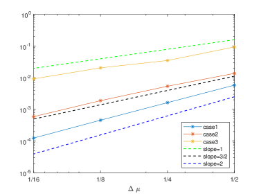
Figure 5 displays the convergence orders of ROM in the slab geometry. The results of different numbers of sampled simulations are shown. To obtain the convergence order of the error, a smaller number of samples is enough. As observed from Figure 5, when the number of samples increases, the convergence order of bias will gradually increase and eventually stabilize near the theoretical value. For different cases as in Example 2.2 in Section 2, Table 2 displays the error and bias using different mesh sizes when there are enough samples.

When the inflow boundary conditions are smooth and regular as in Case 1 in (2.5), the convergence orders of DOM are $2$, while the convergence orders of the error and bias of ROM are respectively $1.37$ and $2.57$. Due to stochastic noise, this can be considered consistent with the analysis. When the boundary conditions are continuous but nondifferentiable as in Case 2 in (2.6), the convergence orders of the DOM decrease to $1.5$, and the convergence orders of the error and bias of ROM remain $1.32$ and $2.92$, respectively. Moreover, if the boundary conditions are discontinuous at some points as in Case 3 in (2.7), the convergence order of DOM decreases to $1$. The convergence order of the error of ROM decreases to $1$, while the bias has a convergence order of $2.37$. In summary, the errors of ROM converge no slower than DOM, and the bias converges faster, especially when the solution regularity is low in the velocity variable.

5.2 The X-Y geometry case

In X-Y geometry, we show the ordinates in the first quadrant and consider uniform partition in the $(\zeta,\theta)$ plane. $\zeta\in[0,1]$ and $\theta\in[0,\pi/2]$ are equally divided, the nodes are denoted by $(\zeta_{i},\theta_{j})=(\frac{N-i+1}{N},\frac{j-1}{2N}\pi)$ for $i,j=1,\cdots,N+1$. Each quadrant has $m=N^{2}$ cells. For any $\ell=(i-1)N+j$, $i,j=1,\cdots,N$,

$$S_{\ell}=\{(\zeta,\theta)|\zeta_{a+1}\leq\zeta\leq\zeta_{a},\theta_{b}\leq\theta\leq\theta_{b+1}.\}$$

Randomly sample $\zeta^{\xi}_{i}\in[\zeta_{i+1},\zeta_{i}]$ and $\theta^{\xi}_{j}\in[\theta_{j},\theta_{j+1}]$ with uniform probability. The ordinates in other quadrant can be obtained by symmetry as in (3.5). The weights are chosen to be $\bar{\omega}_{\ell}=\frac{1}{4N^{2}}$. The ordinates projected to the 2D unit disk are
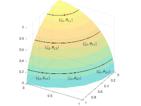
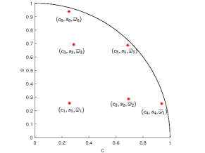
$$(c_{\ell},s_{\ell},\bar{\omega}_{\ell})=\Big{(}\big{(}1-(\zeta^{\xi}_{i})^{2}\big{)}^{\frac{1}{2}}\cos\theta_{j}^{\xi},\big{(}1-(\zeta^{\xi}_{i})^{2}\big{)}^{\frac{1}{2}}\sin\theta_{j}^{\xi},\frac{1}{4N^{2}}\Big{)}.$$

Let’s take $N=3$ as an example, the partition and one sample of the chosen discrete ordinates are plotted in Figure 6.

Refer to caption
Refer to caption
Figure 6: Schematic diagram of selected ordinates on the surface of a 3D unit sphere and their corresponding projection to the 2D unit disk of ROM.

5.2.1 Convergence order

Similar to section 2.2.2, we use the diamond difference method to discretize the spatial variable. The unknowns at the cell centers are calculated, and the notations are the same as in section 2.2.2.

We use the same setup and spatial grid as Example 2.1 in section 2. The numerical error $\mathcal{E}$ and bias $\mathcal{B}$ are similar to (5.1) and (5.2), expect that the $\ell^{2}$ norm is given as in (2.8). The reference solution $\phi^{ref}$ is computed by 80400 ordinates by Gaussian quadrature.

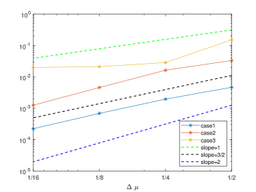
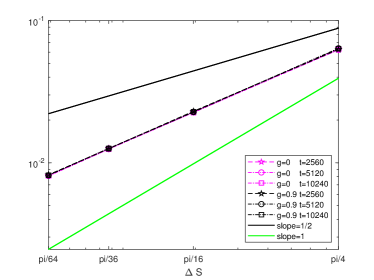
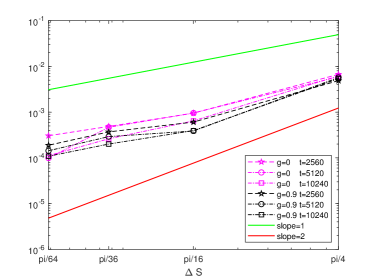
Figure 7 and Table 3 show the convergence order of the error and bias. We can observe that the convergence order of the error is between $0.5$ and $1$, while the convergence order of the bias is between $1$ and $2$ for both isotropic and anisotropic scattering kernels. This is due to the non-smoothness of the solution, which leads to a slight difference between the theoretical value and the actual result.

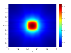
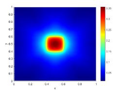
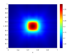
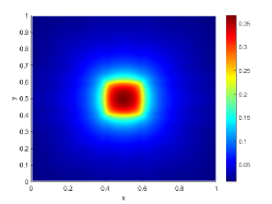
Figure 8 demonstrates the ability of ROM to mitigate the ray effect. The expectation of the average density calculated by ROM with different number of ordinates and different number of sampled simulations are displayed. We can observe that the ray effect is effectively mitigated after multiple parallel calculations and taking the expectations, even when the sampled simulations use a very small number of ordinates. The results with the anisotropic scattering are similar.

Refer to caption
(a) error $\mathcal{E}$
Refer to caption
(b) bias $\mathcal{B}$
Figure 7: The convergence orders of ROM with different velocity meshes in X-Y geometry. Here $\Delta S=\frac{\pi}{4N^{2}}$,$N=1,2,3,4$. (a) the errors ($\mathcal{E}$) for isotropic and anisotropic scattering kernel, (b): the bias ($\mathcal{B}$) for isotropic and anisotropic scattering kernel. S is the number of sampled simulations in ROM.
Table 3: Error, bias and slope of convergence curves in Figure 7 for $t=10240$.
$\Delta S$ $\pi/64$ $\pi/36$ $\pi/16$ $\pi/4$ Order
error ($\mathcal{E})$ iso: g=0 8.09E-03 1.25E-02 2.26E-02 6.28E-02 0.74
aniso: g=0.9 8.18E-03 1.26E-02 2.28E-02 6.36E-02 0.74
bias ($\mathcal{B})$ iso: g=0 1.12E-04 2.62E-04 6.44E-04 6.22E-03 1.44
aniso: g=0.9 1.09E-04 2.01E-04 3.95E-04 5.42E-03 1.41
Refer to caption
(a) 5 simulations, 4 ordinates
Refer to caption
(b) 5 simulations, 16 ordinates
Refer to caption
(c) 5 simulations, 36 ordinates
Refer to caption
(d) 20 simulations, 4 ordinates
Refer to caption
(e) 20 simulations,16 ordinates
Refer to caption
(f) 20 simulations,36 ordinates
Refer to caption
(g) 50 simulations, 4 ordinates
Refer to caption
(h) 50 simulations, 16 ordinates
Refer to caption
(i) 50 simulations, 36 ordinates
Figure 8: Example 2.1(isotropic). The expectation of average density of ROM with different number of sampled simulations and ordinates.

5.2.2 The lattice problem

This example is to demonstrate that the ROM can mitigate the ray effect independent of the problem setup. A benchmark test is the lattice problem in X-Y plane. The spatial domain is $(x,y)\in[0,1]\times[0,1]$ and the cross sections are $\sigma_{T}=1$, $\sigma_{S}=0.5$. The layout of the source term $q(x,y)$ is shown in Figure 9. The number of spatial cells is $50\times 50$ and Diamond difference method is employed for the spatial discretization. In Figure 10, the average densities calculated with $4$, $16$, $36$, $64$, $100$ and $144$ ordinates DOM are displayed. The ray effects can be visually seen even with 144 ordinate.

The results of ROM are shown in Figure 11, where columns 1 to 4 show the expectation of average density $\mathbb{E}\phi^{\xi}$ with 5, 10, 20 and 50 simulations, respectively. As can be seen from the results, the ray effect is invisible in the ROM results when 50 sampled simulations with 4 ordinates, 10 sampled simulations with 16 ordinates, and 5 sampled simulations with 36 ordinates.

Refer to caption
Figure 9: Different source term for lattice problem. The black area is 1, and the other areas are vacant.
Refer to caption
(a) 4 ordinates
Refer to caption
(b) 16 ordinates
Refer to caption
(c) 36 ordinates
Refer to caption
(d) 64 ordinates
Refer to caption
(e) 100 ordinates
Refer to caption
(f) 144 ordinates
Figure 10: The average density of discrete ordinate method with Uniform quadrature.
Refer to caption
(a) t=5, 4 ordinates
Refer to caption
(b) t=10, 4 ordinates
Refer to caption
(c) t=20, 4 ordinates
Refer to caption
(d) t=50, 4 ordinates
Refer to caption
(e) t=5, 9 ordinates
Refer to caption
(f) t=10, 9 ordinates
Refer to caption
(g) t=20, 9 ordinates
Refer to caption
(h) t=50, 9 ordinates
Refer to caption
(i) t=5, 36 ordinates
Refer to caption
(j) t=10, 36 ordinates
Refer to caption
(k) t=20, 36 ordinates
Refer to caption
(l) t=50, 36 ordinates
Figure 11: The expectation of average density of ROM for the lattice problem.

6 Discussion

In the slab geometry, the discontinuities in velocity are usually at fixed velocity directions, thus the decrease in convergence order is not as severe as in the spatial 2D case. On the other hand, the spatial discontinuities or sharp transitions of the inflow boundary conditions and source terms can induce discontinuities in the velocity along the direction of the ray. Thus, the discontinuities in velocity depend on spatial variables for the spatial 2D case. As we can see from Table 1, the commonly used quadrature sets can only achieve a convergence order around $0.74$, which is the main reason for the observed ray effect in spatial 2D test cases.

We remark that other strategies for the random ordinates are possible. For example, $\mathbf{u}_{\ell}$ does not have to be chosen with uniform probability from $S_{\ell}$. One may make use of the transition kernel for importance sampling of $\mathbf{u}_{\ell}$. If these strategies are adopted, the weights $\omega_{\ell}$ have to be adjusted correspondingly. One may consider multiscale total and scattering cross sections as well, then, the conservation of mass may become important. In our future work, we will investigate the extension of ROM to the multiscale cases, such as the diffusion limit or Fokker-Planck limit cases.

Acknowledgments

This work is partially supported by the National Key R&D Program of China No. 2020YFA0712000. The work of L. Li was partially supported by Shanghai Municipal Science and Technology Major Project 2021SHZDZX0102, NSFC 12371400 and 12031013, the Strategic Priority Research Program of Chinese Academy of Sciences, Grant No. XDA25010403.

References

Appendix A Supplementary Materials: Estimates for $\mathcal{T},\mathcal{T}^{\xi},\delta\mathcal{T}^{\xi}$ and $\delta b$

Recall that $\Omega=[x_{L},x_{R}]$, and that the operator $\mathcal{A}_{\mu}(\cdot):L^{2}(\Omega;\sigma_{T})\to L^{2}(\Omega;\sigma_{T})$ maps $\phi(x)$ to $\psi(\cdot,\mu)$ by solving

(A.1) $\displaystyle\mu\partial_{x}\psi+\sigma_{T}\psi=\sigma_{r}\phi,\quad\mu\in[-1,1],$
$\displaystyle\psi(x_{L},\mu)=0,\quad\mu>0;\quad\psi(x_{R},\mu)=0,\quad\mu<0.$

Recall that we have divide the velocity space $S=[-1,0)$ into $n=2m$ cells and the each random ordinates $\mu_{\ell}$, $1\leq\ell\leq m$ is chosen randomly from the $\ell$th cell. The other half $(0,1]$ and the random ordinate $\mu_{\ell+m}$ are chosen in asymmetric fashion. The weight $\omega_{\ell}=|S_{\ell}|/|S|$ and $\alpha_{\ell}=n\omega_{\ell}$. The operator $\mathcal{T}$ is defined as

$$\mathcal{T}=\fint_{S}\mathcal{A}_{\mu}d\mu=\frac{1}{2}\int_{-1}^{1}\mathcal{A}_{\mu}\,d\mu.$$

Let $\mathcal{T}_{\ell}^{\xi}=\alpha_{\ell}\mathcal{A}_{\mu_{\ell}},$ then

$$\mathcal{T}_{\ell}=\mathbb{E}\mathcal{T}_{\ell}^{\xi}=\alpha_{\ell}\fint_{S_{\ell}}\mathcal{A}_{\mu}d\mu=n\omega_{\ell}\frac{1}{|S_{\ell}|}\int_{S_{\ell}}\mathcal{A}_{\mu}d\mu=\frac{n}{|S|}\int_{S_{\ell}}\mathcal{A}_{\mu}d\mu.$$

Therefore, from the definition of $\mathcal{T}_{\ell}$ and $\mathcal{T}_{\ell}^{\xi}$,

(A.2) $$\delta\mathcal{T}^{\xi}:=\mathcal{T}^{\xi}-\mathcal{T}=\frac{1}{m}\sum_{\ell=1}^{m}\frac{1}{2}(\mathcal{T}_{\ell}^{\xi}-\mathcal{T}_{\ell}+\mathcal{T}_{n+1-\ell}^{\xi}-\mathcal{T}_{n+1-\ell})=:\frac{1}{m}\sum_{\ell=1}^{m}\delta\mathcal{T}_{\ell}^{\xi}.$$

Here, we note that $\delta\mathcal{T}_{\ell}^{\xi}$ and $\delta\mathcal{T}_{n+1-\ell}^{\xi}$ are not independent. This is why we put $\ell$ and $n+1-\ell$ together.

For the truncated system, we consider $\mu\in[-1,-\delta)\cup(\delta,1]=:S^{\delta}$. The equation is changed to

$$\mu\partial_{x}\psi+\sigma_{T}\psi=\sigma_{S}\fint_{S^{\delta}}\psi(x,\mu)d\mu+q.$$

We divide $[-1,-\delta)$ and $(\delta,1]$ into $n/2$ subintervals respectively and perform the ROM for the approximation. Then, the weight is changed to $|S_{\ell}|/|S^{\delta}|$. The operators $\mathcal{T}$, $\mathcal{T}^{\xi}$, $\mathcal{T}_{\ell}$, and $\mathcal{T}^{\xi}_{\ell}$ are changed accordingly.

Lemma A.1.

The operator $\mathcal{A}_{\mu}(\cdot)$ satisfies that

(A.3) $$\displaystyle\|\mathcal{A}_{\mu}(\phi)\|_{L^{2}(\Omega;\sigma_{T})}\leq\|\phi\|_{L^{2}(\Omega;\sigma_{T})}\Rightarrow\|\mathcal{A}_{\mu}\|\leq 1,\quad\forall\mu\in[-1,1],$$

and for $\mu\in(-1,0)\cup(0,1)$ that

(A.4) $$\displaystyle\|\partial_{\mu}\mathcal{A}_{\mu}\|\leq\frac{1}{|\mu|}\left(1+\left\|\frac{\sigma_{T}}{\sigma_{r}}\right\|_{\infty}\right).$$

Consequently, $\|\mathcal{T}\|\leq 1$, $\|\mathcal{T}^{\xi}\|\leq 1$, and it holds for the truncated system that

(A.5) $$\|\delta\mathcal{T}_{\ell}^{\xi}\|\leq\frac{C}{\delta}n^{-1}.$$

Proof A.2.

We only consider $\mu\geq 0$ here, as the case for $\mu<0$ is similar. Multiplying $\psi$ in (A.1) and integrating, one has

$$\displaystyle\begin{split}\mu\frac{1}{2}|\psi(x_{R},\mu)|^{2}+\int_{x_{L}}^{x_{R}}\sigma_{T}|\psi|^{2}\,dx&=\int_{x_{L}}^{x_{R}}\sigma_{r}\phi\psi\,dx\leq\int_{x_{L}}^{x_{R}}\sigma_{T}|\phi||\psi|dx\\ &\leq\left(\int_{x_{L}}^{x_{R}}\sigma_{T}|\phi|^{2}\,dx\right)^{1/2}\left(\int_{x_{L}}^{x_{R}}\sigma_{T}|\psi|^{2}dx\right)^{1/2}.\end{split}$$

Hence,

$$\left(\int_{x_{L}}^{x_{R}}\sigma_{T}|\psi|^{2}dx\right)^{1/2}\leq\left(\int_{x_{L}}^{x_{R}}\sigma_{T}|\phi|^{2}\,dx\right)^{1/2},$$

which implies that $\|\mathcal{A}_{\mu}\|\leq 1$.

Taking the derivative of both sides of (A.1) with respect to $\mu$

$$\partial_{x}\psi+\mu\partial_{x}(\partial_{\mu}\psi)+\sigma_{T}\partial_{\mu}\psi=0,\quad\partial_{\mu}\psi(x_{L},\mu)=0.$$

Hence, one has

$$\partial_{\mu}\psi=\mathcal{A}_{\mu}(-\partial_{x}\psi/\sigma_{r})=-\mathcal{A}_{\mu}\left(\mu^{-1}(\phi-\frac{\sigma_{T}}{\sigma_{r}}\psi)\right).$$

By (A.3), one then has

$$\|\partial_{\mu}\psi\|\leq\mu^{-1}\|\phi-\frac{\sigma_{T}}{\sigma_{r}}\mathcal{A}_{\mu}(\phi)\|\leq\mu^{-1}(\|\phi\|+\|\frac{\sigma_{T}}{\sigma_{r}}\|_{\infty}\|\phi\|).$$

The inequality (A.4) holds.

Since $\mathcal{T}^{\xi}$ and $\mathcal{T}$ are the averages of $\mathcal{A}_{\mu}$, the second claims are straightforward. For the truncated system, one has

$$\delta\mathcal{T}^{\xi}=\alpha_{\ell}|S_{\ell}|^{-1}\int_{S_{\ell}}\mathcal{A}_{\mu}-\mathcal{A}_{\mu_{\ell}}d\mu,$$

then

$$\|\delta\mathcal{T}_{\ell}^{\xi}\|\leq\alpha_{\ell}\sup_{\mu\in S_{\ell}\cup S_{\ell+m}}\|\partial_{\mu}\mathcal{A}_{\mu}\||S_{\ell}|=n^{-1}|S|\alpha_{\ell}^{2}\sup_{\mu\in S_{\ell}\cup S_{\ell+m}}\|\partial_{\mu}\mathcal{A}_{\mu}\|.$$

The claim then follows.

Next, our main goal is to estimate $\mathbb{E}\|\delta\mathcal{T}^{\xi}\|^{2}$ where $\delta\mathcal{T}^{\xi}$ is given in (A.2).

If the independent random variables $\delta\mathcal{T}_{\ell}^{\xi}$ take values in a Hilbert space, some classical concentration inequalities like the Rosenthal inequality [30] can be used to achieve this. However, here the variables are operators over Hilbert spaces so they are in a Banach algebra. One cannot apply the classical Rosenthal inequality directly. Our goal in this section is then to establish a Rosenthal type inequality for these operator-valued random variables.

First, we observe the following

$$\mathbb{E}\|\delta\mathcal{T}^{\xi}\|^{2}\leq\mathbb{E}\big{|}\|\delta\mathcal{T}^{\xi}\|-\mathbb{E}\|\delta\mathcal{T}^{\xi}\|\big{|}^{2}+(\mathbb{E}\|\delta\mathcal{T}^{\xi}\|)^{2}.$$

The first term on the right-hand side can be estimated by the following fact.

Lemma A.3.

For any separable Banach space $B$ and any finite sequence of independent $B$-valued random vectors $X_{j}$, $1\leq j\leq m$ with $\mathbb{E}\|X_{j}\|^{2}<\infty$. Let $S_{m}=\sum_{j=1}^{m}X_{j}$. Then,

$$\mathbb{E}\big{|}\left\|S_{m}\right\|-\mathbb{E}\left\|S_{m}\right\|\big{|}^{2}\leq 4\sum_{j=1}^{m}\mathbb{E}\left\|X_{j}\right\|^{2}.$$

This result is a special case of [1, Theorem 2.1], where the general $L^{p}$ case is considered. The proof is a consequence of the Birkholder inequality for martingales. Here, we sketch the proof for the special case here. Consider the filtration $\{\mathcal{F}_{j},0\leq j\leq m\}$ where

$$\mathcal{F}_{j}=\sigma(X_{\ell}:1\leq\ell\leq j),1\leq j\leq m,$$

and $\mathcal{F}_{0}=\{\Omega,\emptyset\}$. Define $Y_{j}=\mathbb{E}(\|S_{m}\||\mathcal{F}_{j})-\mathbb{E}(\|S_{m}\||\mathcal{F}_{j-1})$, where $\mathbb{E}(\|S_{m}\||\mathcal{F}_{0}):=\mathbb{E}(\|S_{m}\|)$. Then, one has

$$\displaystyle\mathbb{E}\big{|}\left\|S_{m}\right\|-\mathbb{E}\left\|S_{m}\right\|\big{|}^{2}=\mathbb{E}|\sum_{j=1}^{m}Y_{j}|^{2}=\sum_{j=1}^{m}\mathbb{E}(|Y_{j}|^{2}).$$

By the definition, one has

$$|Y_{j}|=\Bigg{|}\mathbb{E}_{X_{1},\cdots,X_{j-1},X_{j}^{\prime}}\|X_{1}+\cdots+X_{j-1}+X_{j}^{\prime}+X_{j+1}+\cdots\|\\ -\mathbb{E}_{X_{1},\cdots,X_{j-1}}\|X_{1}+\cdots+X_{j-1}+X_{j}+X_{j+1}+\cdots\|\Bigg{|}\leq\mathbb{E}_{X_{j}^{\prime}}|X_{j}^{\prime}-X_{j}|.$$

Here $X_{j}^{\prime}$ is an independent copy of $X_{j}$. This then gives that $\mathbb{E}|Y_{j}|^{2}\leq 4\mathbb{E}(\|X_{j}\|^{2})$.

Hence, the problem is reduced to estimation of $\mathbb{E}\|\delta\mathcal{T}^{\xi}\|$. We will mainly make use the approach in [34]. The analysis in [34] is for matrices and the final result relies on the dimension of the space. In our case, the operator is in an infinite dimensional space. We find that the dependence on the dimension is due to the trace of the operators. Fortunately, for our case, the operator is compact and we could possibly bound the trace.

Firstly, we introduce the Mercer’s theorem about trace class mentioned in [20, Sec. 30.5, Theorem 11].

Lemma A.4.

Consider an integral operator $\boldsymbol{K}$ of the form

$$(\boldsymbol{K}u)(s)=\int_{I}K(s,t)u(t)w(t)dt$$

acting on $L^{2}(I;w)$, where $K$ is a real-valued symmetric, continuous function of $(s,t)$ and $w(t)$ is a continuous positive weight. Then, the operator $\boldsymbol{K}$ is positive in the usual sense:

$$(\boldsymbol{K}u,u)\geq 0,\quad\text{for all $u$ in $L^{2}(I;w)$},$$

and is of trace class with the trace equal to the integral of its kernel along the diagonal:

$$\operatorname{tr}(\boldsymbol{K})=\int_{I}K(s,s)w(s)ds.$$

The result in [20, Sec. 30.5, Theorem 11] is about the uniform weight $w=1$. It is not hard to check that the proof holds for general continuous positive weight on $I$. Based on the above lemma, we naturally deduce the following proposition.

Proposition A.5.

For any $\mu\neq 0$, $\mathcal{A}_{\mu}$ is a compact operator. $\mathcal{A}_{\mu}^{*}$ is the adjoint operator of $\mathcal{A}_{\mu}$, then $\mathcal{A}_{\mu}^{*}\mathcal{A}_{\mu}$ and $\mathcal{A}_{\mu}\mathcal{A}_{\mu}^{*}$ are in the trace class. Moreover,

$$\operatorname{tr}\mathcal{A}_{\mu}^{*}\mathcal{A}_{\mu}=\operatorname{tr}\mathcal{A}_{\mu}\mathcal{A}_{\mu}^{*}\leq\frac{1}{|\mu|}|x_{R}-x_{L}|\|\sigma_{T}\|_{\infty}^{2}\|\sigma_{T}^{-1}\|_{\infty}.$$

Proof A.6.

According to [20], an integral operator $L^{2}(I;w)\to L^{2}(I;w)$ with a square integrable kernel is compact. The first claim follows directly by the solution in expanded form.

We only consider $\mu>0$ and the proof for $\mu<0$ is similar. By the definition of adjoint operators, $\langle\mathcal{A}_{\mu}g,h\rangle=\langle g,\mathcal{A}_{\mu}^{*}h\rangle$, one finds that

$$(\mathcal{A}_{\mu}^{*}\varphi)(x)=\int_{x_{L}}^{x_{R}}\tilde{k}_{\mu}(x,y)\varphi(y)\sigma_{T}(y)dy,\quad\tilde{k}_{\mu}(x,y)=k_{\mu}(y,x).$$

Then, one has

$$\mathcal{A}_{\mu}\mathcal{A}_{\mu}^{*}\varphi=\int_{x_{L}}^{x_{R}}K_{1}(x,y)\varphi(y)\sigma_{T}(y)dy,\quad K_{1}(x,y)=\int_{x_{L}}^{x_{R}}k_{\mu}(x,z)\tilde{k}_{\mu}(z,y)\sigma_{T}(z)dz.$$

Similarly,

$$\mathcal{A}_{\mu}^{*}\mathcal{A}_{\mu}\varphi=\int_{x_{L}}^{x_{R}}K_{2}(x,y)\varphi(y)\sigma_{T}(y)dy,\quad K_{2}(x,y)=\int_{x_{L}}^{x_{R}}\tilde{k}_{\mu}(x,z)k_{\mu}(z,y)\sigma_{T}(z)dz.$$

Hence,

(A.6a) $\displaystyle K_{1}(x,y)=\int_{x_{L}}^{\min(x,y)}\frac{1}{\mu^{2}}\frac{\sigma_{r}^{2}(z)}{\sigma_{T}(z)}\exp\left(-\frac{1}{\mu}(\int_{z}^{x}\sigma_{T}(w)dw+\int_{z}^{y}\sigma_{T}(w)dw)\right)$ $\displaystyle dz$
(A.6b) $\displaystyle K_{2}(x,y)=\int_{\max(x,y)}^{x_{R}}\frac{1}{\mu^{2}}\frac{\sigma_{r}(x)\sigma_{r}(y)}{\sigma_{T}(x)\sigma_{T}(y)}\exp\left(-\frac{1}{\mu}(\int_{x}^{z}\sigma_{T}(w)dw+\int_{y}^{z}\sigma_{T}(w)dw)\right)\sigma_{T}(z)$ $\displaystyle dz.$

According to these two formulas, it is clear that both kernels are continuous in $(x,y)$.

Repeating the Lemma A.4, it is easy to find that both operators are in trace class and

$$\operatorname{tr}(\mathcal{A}_{\mu}\mathcal{A}_{\mu}^{*})=\int_{x_{L}}^{x_{R}}K_{1}(x,x)\sigma_{T}(x)dx,\quad\operatorname{tr}(\mathcal{A}_{\mu}^{*}\mathcal{A}_{\mu})=\int_{x_{L}}^{x_{R}}K_{2}(x,x)\sigma_{T}(x)dx.$$

These two traces are in fact equal by (A.6) and Fubini’s theorem, and are equal to

$$\int_{x_{L}}^{x_{R}}\int_{x_{L}}^{x_{R}}|k_{\mu}(x,y)|^{2}\sigma_{T}(x)\sigma_{T}(y)dxdy.$$

Then, one finds

(A.7) $$\begin{split}&\operatorname{tr}(\mathcal{A}_{\mu}\mathcal{A}_{\mu}^{*})=\operatorname{tr}(\mathcal{A}_{\mu}^{*}\mathcal{A}_{\mu})\\ &\leq\frac{1}{\mu^{2}}\|\sigma_{T}\|_{\infty}^{2}\int_{x_{L}}^{x_{R}}\int_{x_{L}}^{x_{R}}\mathbb{I}_{z\leq x}\exp\left(-\frac{2}{\mu}\frac{1}{\|\sigma_{T}^{-1}\|_{\infty}}(x-z)\right)dxdz\\ &\leq\frac{1}{\mu}|x_{R}-x_{L}|\|\sigma_{T}\|_{\infty}^{2}\|\sigma_{T}^{-1}\|_{\infty}.\end{split}$$

The case for $\mu<0$ is similar, omitted.

We adopt the argument in [34] to our case for $\mathbb{E}\|\delta\mathcal{T}^{\xi}\|$.

First, define the symmetrization of the operators. Because $\delta\mathcal{T}^{\xi}$ is not a self-adjoint operator, we let $\delta\mathcal{H}$ be the symmetrization operator of $\delta\mathcal{T}^{\xi}$, given by

$$\displaystyle\delta\mathcal{H}=\frac{1}{m}\sum_{\ell=1}^{m}\delta\mathcal{H}_{\ell}.$$

where

$$\displaystyle\delta\mathcal{H}_{\ell}:=\left[\begin{array}[]{cc}0&\delta\mathcal{T}_{\ell}^{\xi}\\ (\delta\mathcal{T}_{\ell}^{\xi})^{*}&0\end{array}\right].$$

Clearly, each $\delta\mathcal{H}_{\ell}$ are operators in $(L^{2}(\sigma_{T}))^{\otimes 2}\to(L^{2}(\sigma_{T}))^{\otimes 2}$. The symmetrization has a good property that is

(A.8) $$\displaystyle\|\delta\mathcal{T}_{\ell}^{\xi}\|=\|\delta\mathcal{H}_{\ell}\|,\quad\|\delta\mathcal{T}^{\xi}\|=\|\delta\mathcal{H}\|.$$

In fact, since $\delta\mathcal{H}_{\ell}$ is a self-adjoint operator, and

$\displaystyle\|\delta\mathcal{H}_{\ell}\|^{2}$ $\displaystyle=\|\delta\mathcal{H}_{\ell}^{2}\|=\Bigg{\|}\left[\begin{array}[]{cc}\delta\mathcal{T}_{\ell}^{\xi}(\delta\mathcal{T}_{\ell}^{\xi})^{*}&0\\ 0&(\delta\mathcal{T}_{\ell}^{\xi})^{*}\delta\mathcal{T}_{\ell}^{\xi}\end{array}\right]\Bigg{\|}$
$\displaystyle=\max\{\|\delta\mathcal{T}_{\ell}^{\xi}(\delta\mathcal{T}_{\ell}^{\xi})^{*}\|,\|(\delta\mathcal{T}_{\ell}^{\xi})^{*}\delta\mathcal{T}_{\ell}^{\xi}\|\}=\|\delta\mathcal{T}_{\ell}^{\xi}\|^{2}.$

The other relation $\|\delta\mathcal{T}^{\xi}\|=\|\delta\mathcal{H}\|$ follows from the same argument. Hence, it reduces to estimate $\|\delta\mathcal{H}\|$.

Next, we consider the Rademacher symmetrization:

$$\displaystyle\delta\mathcal{H}^{\epsilon}=\frac{1}{m}\sum_{{\ell}=1}^{m}\epsilon_{\ell}\delta\mathcal{H}_{\ell},$$

where $\epsilon_{\ell}$ are independent Rademacher random variables (i.e., indepedent Bernoulli variables taking values in $\{-1,1\}$). Introduction of $\epsilon_{\ell}$ brings extra randomness to utilize the independence. The following is well-known (see [34, Fact 3.1]), which indicates that introduction of $\epsilon_{\ell}$ would not lose control of the random variables.

Lemma A.7.

The Rademacher symmetrization satisfies

$$\frac{1}{2}\mathbb{E}\|\delta\mathcal{H}^{\epsilon}\|\leq\mathbb{E}\|\delta\mathcal{H}\|\leq 2\mathbb{E}\|\delta\mathcal{H}^{\epsilon}\|,$$

where $\mathbb{E}$ means that the expectation is with respect to all randomness, including those in Rademacher variables and random ordinates.

The following estimate gives the control by taking the expectation over $\epsilon_{\ell}$, following the approach in [34].

Lemma A.8.

It holds that

$$\mathbb{E}_{\epsilon}\|\delta\mathcal{H}^{\epsilon}\|\leq\sqrt{3+2\left[\log\frac{m^{-1}\sum_{\ell}\operatorname{tr}\left(\delta\mathcal{H}_{\ell}^{2}\right)}{m^{-1}\sum_{\ell}\|\delta\mathcal{H}_{\ell}^{2}\|}\right]}\left(\frac{1}{m^{2}}\sum_{\ell}\|\delta\mathcal{H}_{\ell}^{2}\|\right)^{1/2},$$

where $\mathbb{E}_{\epsilon}$ means the expectation over the Rademacher variables.

Proof A.9.

Note that $\delta\mathcal{H}^{\epsilon}$ is self-adjoint, and $(\delta\mathcal{H}^{\epsilon})^{2}$ is nonnegative and compact. Hence, $\|\delta\mathcal{H}^{\epsilon}\|^{2p}=\|(\delta\mathcal{H}^{\epsilon})^{2p}\|$ for each nonnegative integer $p$ so that

$$\mathbb{E}_{\epsilon}\|\delta\mathcal{H}^{\epsilon}\|\leq(\mathbb{E}_{\epsilon}\left\|(\delta\mathcal{H}^{\epsilon})^{2p}\right\|)^{1/(2p)}\leq\left[\mathbb{E}_{\epsilon}\operatorname{tr}\left((\delta\mathcal{H}^{\epsilon})^{2p}\right)\right]^{1/(2p)}.$$

The above holds because the norm of $(\delta\mathcal{H}^{\epsilon})^{2}$ is the largest eigenvalue while the trace is the sum of all eigenvalues. For each index $\ell\in\{1,\cdots,m\}$, define the random operators

$$\delta\mathcal{H}_{+\ell}:=\frac{1}{m}\delta H_{\ell}+\frac{1}{m}\sum_{j\neq\ell}\epsilon_{j}\delta\mathcal{H}_{j}\quad\text{ and }\quad\delta\mathcal{H}_{-\ell}:=-\frac{1}{m}\delta\mathcal{H}_{\ell}+\frac{1}{m}\sum_{j\neq\ell}\epsilon_{j}\delta\mathcal{H}_{j}.$$

Denote $\hat{\epsilon}_{\ell}=\{\epsilon_{1},\cdots,\epsilon_{\ell-1},\epsilon_{\ell+1},\cdots,\epsilon_{m}\}$. Then, it holds that

$\displaystyle\mathbb{E}_{\epsilon}\operatorname{tr}\left((\delta\mathcal{H}^{\epsilon})^{2p}\right)$ $\displaystyle=\frac{1}{2}\sum_{\ell}\mathbb{E}_{\hat{\epsilon}_{\ell}}\operatorname{tr}\left(\frac{1}{m}\delta\mathcal{H}_{\ell}\left(\delta\mathcal{H}_{+\ell}^{2p-1}-\delta\mathcal{H}_{-\ell}^{2p-1}\right)\right)$
$\displaystyle=\frac{1}{m^{2}}\sum_{\ell=1}^{m}\sum_{j=0}^{2p-2}\mathbb{E}_{\hat{\epsilon}_{\ell}}\operatorname{tr}\left(\delta\mathcal{H}_{\ell}\delta\mathcal{H}_{+\ell}^{j}\delta\mathcal{H}_{\ell}\delta\mathcal{H}_{-\ell}^{2p-2-j}\right)$
$\displaystyle\leq\frac{1}{m^{2}}\sum_{\ell=1}^{m}\frac{2p-1}{2}\mathbb{E}_{\hat{\epsilon}_{\ell}}\operatorname{tr}\left[\delta\mathcal{H}_{\ell}^{2}\cdot\left(\delta\mathcal{H}_{+\ell}^{2p-2}+\delta\mathcal{H}_{-\ell}^{2p-2}\right)\right]$
$\displaystyle=(2p-1)\operatorname{tr}\left[\frac{1}{m^{2}}\left(\sum_{\ell=1}^{m}\delta\mathcal{H}_{\ell}^{2}\right)\mathbb{E}_{\epsilon}(\delta\mathcal{H}^{\epsilon})^{2p-2}\right].$

The second line is due to the equality

$$\delta\mathcal{H}_{+\ell}^{2p-1}-\delta\mathcal{H}_{-\ell}^{2p-1}=\sum_{q=0}^{2p-2}\delta\mathcal{H}_{+\ell}^{q}(\delta\mathcal{H}_{+\ell}-\delta\mathcal{H}_{-\ell})\delta\mathcal{H}_{-\ell}^{2p-2-q},$$

and $\delta\mathcal{H}_{+\ell}-\delta\mathcal{H}_{-\ell}=\frac{2}{m}\delta\mathcal{H}_{\ell}$. The third line is due to the following Geometric Mean-Arithmetic Mean (GM-AM) trace inequality in [34, Fact 2.4]

(A.9) $$\displaystyle\operatorname{tr}(HW^{q}HY^{2r-q})+\operatorname{tr}(HW^{2r-q}HY^{q})\leq\operatorname{tr}(H^{2}(W^{2r}+Y^{2r})),$$

which can be generalized to self-adjoint compact operators in trace class. Here, $q,r$ are integers and $0\leq q\leq 2r$, and $H,W$ are two arbitrary self-adjoint compact operators in trace class. In fact, one can approximate the compact operators using finite rank self-adjoint operators, and the finite rank operators (essentially matrices) satisfy (A.9). Passing the limit for the finite rank approximation then verifies the inequality for self-adjoint compact operators. The last line follows since $\delta\mathcal{H}_{+\ell}^{2p-2}+\delta\mathcal{H}_{-\ell}^{2p-2}=2\mathbb{E}_{\epsilon_{\ell}}(\delta\mathcal{H}^{\epsilon})^{2p-2}$.

Recall that (see [20, section 30.2, Theorem 2]) if $A$ is self-adjoint, nonnegative and in trace class, then $\|A\|_{\operatorname{tr}}=\operatorname{tr}(A)$ and

(A.10) $$\displaystyle\operatorname{tr}(AB)\leq\|AB\|_{\operatorname{tr}}\leq\|B\|\|A\|_{\operatorname{tr}}=\|B\|\operatorname{tr}(A).$$

Applying (A.10) and repeating the above process, one then has

$$\begin{split}\mathbb{E}_{\epsilon}\operatorname{tr}\left((\delta\mathcal{H}^{\epsilon})^{2p}\right)&\leq(2p-1)\left\|\frac{1}{m^{2}}\left(\sum_{\ell=1}^{m}\delta H_{\ell}^{2}\right)\right\|\mathbb{E}_{\epsilon}\operatorname{tr}(\delta\mathcal{H}^{\epsilon})^{2p-2}\\ &\leq(2p-1)!!\left\|\frac{1}{m^{2}}\left(\sum_{\ell=1}^{m}\delta H_{\ell}^{2}\right)\right\|^{p-1}\mathbb{E}_{\epsilon}\operatorname{tr}(\delta\mathcal{H}^{\epsilon})^{2}.\end{split}$$

Since

$$\mathbb{E}_{\epsilon}(\delta\mathcal{H}^{\epsilon})^{2}=\frac{1}{m^{2}}\sum_{\ell}\delta\mathcal{H}_{\ell}^{2}$$

and $(2p-1)!!\leqslant\left(\frac{2p+1}{\mathrm{e}}\right)^{p}$, we then arrive at

$$\mathbb{E}_{\epsilon}\|\delta\mathcal{H}^{\epsilon}\|\leq\sqrt{\frac{2p+1}{e}}\left(\frac{1}{m^{2}}\sum_{\ell}\|\delta\mathcal{H}_{\ell}^{2}\|\right)^{1/2-1/(2p)}\left(\frac{1}{m^{2}}\sum_{\ell}\operatorname{tr}\left(\delta\mathcal{H}_{\ell}^{2}\right)\right)^{1/(2p)}.$$

Taking

$$p=\left[\log\frac{\sum_{\ell}\operatorname{tr}\left(\delta\mathcal{H}_{\ell}^{2}\right)}{\sum_{\ell}\|\delta\mathcal{H}_{\ell}^{2}\|}\right]+1$$

gives the result.

Combining Lemma A.3 and Lemma A.8, we conclude a Rosenthal type inequality for $\delta\mathcal{T}^{\xi}$.

Theorem A.10.

For $p=2$, $\delta\mathcal{T}^{\xi}$ defined in (A.2), it holds that

(A.11) $$\displaystyle\mathbb{E}(\|\delta\mathcal{T}^{\xi}\|^{2})\leq 8\mathbb{E}\left[\left(\log\frac{m^{-1}\sum_{\ell}\operatorname{tr}\left((\delta\mathcal{T}_{\ell}^{\xi})^{*}\delta\mathcal{T}_{\ell}^{\xi}\right)}{m^{-1}\sum_{\ell}\|\delta\mathcal{T}_{\ell}^{\xi}\|^{2}}+2.7\right)\frac{1}{m^{2}}\sum_{\ell=1}^{m}\|\delta\mathcal{T}_{\ell}^{\xi}\|^{2}\right].$$

Proof A.11.

By Lemma A.7, one finds that

$$\mathbb{E}\|\delta\mathcal{T}^{\xi}\|=\mathbb{E}\|\delta\mathcal{H}\|\leq 2\mathbb{E}\|\delta\mathcal{H}^{\epsilon}\|=2\mathbb{E}(\mathbb{E}_{\epsilon}\|\delta\mathcal{H}^{\epsilon}\|).$$

Then according to Lemma A.3 and Lemma A.8, one has

$$\begin{split}\mathbb{E}(\|\delta\mathcal{T}^{\xi}\|^{2})&\leq(\mathbb{E}\|\delta\mathcal{T}^{\xi}\|)^{2}+4\sum_{\ell=1}^{m}\frac{1}{m^{2}}\mathbb{E}\|\delta\mathcal{T}_{\ell}^{\xi}\|^{2}\\ &\leq 4\mathbb{E}\left[\left(4+2\log\frac{m^{-1}\sum_{\ell}\operatorname{tr}\left((\delta\mathcal{T}_{\ell}^{\xi})^{*}\delta\mathcal{T}_{\ell}^{\xi}\right)}{m^{-1}\sum_{\ell}\|\delta\mathcal{T}_{\ell}^{\xi}\|^{2}}+2\log 2\right)\frac{1}{m^{2}}\sum_{\ell}\|\delta\mathcal{T}_{\ell}^{\xi}\|^{2}\right],\end{split}$$

where we have used $[x]\leq x$. Since $2\log 2<1.4$, the result follows.

We conclude the following.

Corollary A.12 (Bounds of $\mathbb{E}\|\delta\mathcal{T}^{\xi}\|^{2}$).

It holds for the truncated system that

$$\displaystyle\mathbb{E}(\|\delta\mathcal{T}^{\xi}\|^{2})\leq C(\log n+1)n^{-3},$$

where $C$ is a constant that is independent of $n$.

Proof A.13.

In (A.11), we note that

$$\mathbb{E}\operatorname{tr}((\delta\mathcal{T}_{\ell}^{\xi})^{*}\delta\mathcal{T}_{\ell})=\mathbb{E}\operatorname{tr}((\bar{\mathcal{T}}_{\ell}^{\xi})^{*}\bar{\mathcal{T}}_{\ell}^{\xi})-\operatorname{tr}(\bar{\mathcal{T}}_{\ell}^{*}\bar{\mathcal{T}}_{\ell})\leq\mathbb{E}\operatorname{tr}((\bar{\mathcal{T}}_{\ell}^{\xi})^{*}\bar{\mathcal{T}}_{\ell}^{\xi}),$$

where $\bar{\mathcal{T}}_{\ell}=\frac{1}{2}(\mathcal{T}_{\ell}+\mathcal{T}_{\ell+m})$ and $\bar{\mathcal{T}}_{\ell}^{\xi}$ is similarly defined. The inequality above holds because $\operatorname{tr}(\bar{\mathcal{T}}_{\ell}^{*}\bar{\mathcal{T}}_{\ell})=\operatorname{tr}(\bar{\mathcal{T}}_{\ell}\bar{\mathcal{T}}_{\ell}^{*})\geq 0$. Moreover, using the simple control,

$$\operatorname{tr}(T_{1}T_{2}^{*}+T_{2}T_{1}^{*})\leq\operatorname{tr}(T_{1}T_{1}^{*}+T_{2}T_{2}^{*}),\quad\operatorname{tr}(T_{1}^{*}T_{2}+T_{2}^{*}T_{1})\leq\operatorname{tr}(T_{1}^{*}T_{1}+T_{2}^{*}T_{2})$$

we conclude that by Lemma A.5 for the truncated system that

$$n^{-1}\sum_{\ell}\operatorname{tr}(\delta\mathcal{T}_{\ell}^{\xi})^{*}\delta\mathcal{T}_{\ell}^{\xi}\leq C.$$

Moreover, by Lemma A.1 and noting $n=2m$,

$$\frac{1}{m^{2}}\sum_{\ell}\|\delta\mathcal{T}_{\ell}^{\xi}\|^{2}\leq C\frac{1}{n^{3}},\quad|\log(m^{-1}\sum_{\ell}\|\delta\mathcal{T}_{\ell}^{\xi}\|^{2})|\leq C(1+\log n).$$

The claim then follows.

Next, we move to the estimation of $\|\delta b(x)\|$, which is much easier than $\delta\mathcal{T}^{\xi}$ since it is in the Hilbert space $L^{2}(\sigma_{T})$. Here, we prove the lemma without truncation (the truncated version is clearly correct if the un-truncated one holds).

Lemma A.14.

Suppose that $\mu\mapsto\psi_{\mu}(x_{L})$ is Lipschitz on $(-1,0)$ and $\mu\mapsto\psi_{\mu}(x_{R})$ is Lipschitz on $(0,1)$. Then, it holds that

$$\mathbb{E}\|\delta b\|_{L^{2}(\sigma_{T})}\leq C\sqrt{n^{-3}(1+\log n)},$$

where $C$ is a constant that is independent of $n$.

Proof A.15.

By the Hölder inequality

$$\mathbb{E}\|\delta b\|\leq\sqrt{\mathbb{E}\|\delta b\|^{2}}.$$

Define $\tilde{b}_{\ell}:=b_{\mu_{\ell}}+b_{\mu_{\ell+m}}$. Then it holds that

(A.12) $\displaystyle\mathbb{E}\|\delta b\|^{2}$ $\displaystyle=\mathbb{E}\Big{\|}\frac{1}{n}\sum_{\ell}\alpha_{\ell}b_{\mu_{\ell}}-\frac{1}{2}\int_{-1}^{1}b_{\mu}d\mu\Big{\|}^{2}=\mathbb{E}\Big{\|}\sum_{\ell=1}^{m}\left(\omega_{\ell}\tilde{b}_{\ell}-\frac{1}{|S|}\int_{S_{\ell}\cup S_{\ell+m}}b_{\mu}d\mu\right)\Big{\|}^{2}$
$\displaystyle=\sum_{\ell=1}^{m}\mathbb{E}\Big{\|}\omega_{\ell}\tilde{b}_{\ell}-\frac{1}{|S|}\int_{S_{\ell}\cup S_{\ell+m}}b_{\mu}d\mu\Big{\|}^{2}$
$\displaystyle=\frac{1}{|S|^{2}}\sum_{\ell=1}^{m}\mathbb{E}\Big{\|}\int_{S_{\ell}}(b_{\mu_{\ell}}-b_{\mu})d\mu+\int_{S_{\ell+m}}(b_{\mu_{\ell+m}}-b_{\mu})d\mu\Big{\|}^{2}$
$\displaystyle\leq\frac{2}{|S|^{2}}\sum_{\ell=1}^{n}\mathbb{E}\left(\int_{S_{\ell}}\|b_{\mu_{\ell}}-b_{\mu}\|d\mu\right)^{2}\leq\sum_{\ell=1}^{n}\frac{2|S_{\ell}|}{|S|^{2}}\mathbb{E}\int_{S_{\ell}}\|b_{\mu_{\ell}}-b_{\mu}\|^{2}d\mu.$

Above, the summation can be moved out of the norm because the expectation of the cross terms are zero, i.e.,

$$\mathbb{E}\left(\omega_{\ell}\tilde{b}_{\ell}-\frac{1}{|S|}\int_{S_{\ell}\cup S_{\ell+m}}b_{\mu}d\mu\right)\left(\omega_{\ell^{\prime}}\tilde{b}_{\mu_{\ell^{\prime}}}-\frac{1}{|S|}\int_{S_{\ell^{\prime}}\cup S_{\ell^{\prime}+m}}b_{\mu}d\mu\right)=0$$

for $\ell\neq\ell^{\prime}$. The last inequality is due to the Hölder inequality.

Using the explicit formula of $b_{\mu}$, we will show now for $\ell=1,\cdots,m$ and $\mu\in S_{\ell}$ that

(A.13) $$\|b_{\mu_{\ell}}-b_{\mu}\|^{2}\leq\begin{cases}C\frac{1}{|\mu|n^{2}}&\inf\{|\mu|:\mu\in S_{\ell}\}\geq 2n^{-1},\\ Cn^{-1}&\text{otherwise}.\\ \end{cases}$$

Below, we consider only $\mu>0$ ($\mu<0$ is similar). Recall the boundary propagator for $\mu>0$:

$$\displaystyle B_{\mu}(x)=\exp\left(-\frac{1}{\mu}\int_{x_{L}}^{x}\sigma_{T}(y)\,dy\right).$$

Clearly, for $\mu_{1},\mu_{2}\in S_{\ell}$, $\mu_{1}>0,\mu_{2}>0$ and $\mu_{1}<\mu_{2}$, one has $\delta\mu:=\mu_{2}-\mu_{1}\leq\alpha_{\ell}|S|/n$ and thus

$$\|b_{\mu_{1}}-b_{\mu_{2}}\|^{2}\leq 2\|B_{\mu_{1}}(\cdot)-B_{\mu_{2}}(\cdot)\|^{2}\sup_{\mu}|\psi(x_{L},\mu)|+2\alpha_{\ell}^{2}|S|^{2}\|B_{\mu_{2}}(\cdot)\|^{2}L_{\psi}^{2}n^{-2},$$

where $L_{\psi}$ is the Lipschitz constant of $\psi$.

Let $M(x)=\int_{x_{L}}^{x}\sigma_{T}(y)dy$. Note the simple fact

$$B_{\mu_{1}}(x)-B_{\mu_{2}}(x)=\exp\left(-\frac{M(x)}{\mu_{2}}\right)\left(\exp\left(-\frac{M(x)\delta\mu}{\mu_{1}\mu_{2}}\right)-1\right).$$

If $\inf\{\mu:\mu\in S_{\ell}\}<2/n$, since $\alpha_{\ell}$ is bounded, $\mu_{2}\leq C/n$ for some constant $C>0$. Since $|\exp\left(-\frac{M(x)\delta\mu}{\mu_{1}\mu_{2}}\right)-1|<1$, one has

$$\left\|B_{\mu_{1}}(\cdot)-B_{\mu_{2}}(\cdot)\right\|^{2}\leq\left\|\exp\left(-\frac{M(x)}{\mu_{2}}\right)\right\|^{2}\leq Cn^{-1}.$$

If $\inf\{\mu:\mu\in S_{\ell}\}\geq 2/n$, then $\mu_{2}/\mu_{1}=1+\delta\mu/\mu_{1}$ is bounded. Using the simple bound $|\exp\left(-\frac{M(x)\delta\mu}{\mu_{1}\mu_{2}}\right)-1|\leq M(x)\delta\mu/(\mu_{1}\mu_{2})$, one has

$$\begin{split}\left\|B_{\mu_{1}}(\cdot)-B_{\mu_{2}}(\cdot)\right\|^{2}&\leq\int_{x_{L}}^{x_{R}}\frac{\delta\mu^{2}}{\mu_{1}^{2}\mu_{2}^{2}}M^{2}(x)\exp\left(-\frac{2M(x)}{\mu_{2}}\right)\sigma_{T}(x)dx\\ &\leq C\frac{\mu_{2}}{n^{2}\mu_{1}^{2}}\leq C^{\prime}\frac{1}{\mu_{1}n^{2}}.\end{split}$$

The second inequality here follows by the substitution $w=x/\mu_{2}$ and the fact

$$z^{2}\exp(-2z)\leq Ce^{-z}.$$

Hence, (A.13) is proved.

By (A.13), one finds easily that (A.12) is controlled by

$$\mathbb{E}\|\delta b\|^{2}\leq C\frac{1}{n^{2}}\sum_{\ell:\inf\{\mu:\mu\in S_{\ell}\}<2/n}|S_{\ell}|+C\frac{1}{n}\int_{2n^{-1}}^{1}\frac{1}{n^{2}\mu}d\mu$$

and thus the result follows.