Subequivariant Reinforcement Learning
in 3D Multi-Entity Physical Environments

Abstract

Learning policies for multi-entity systems in 3D environments is far more complicated against single-entity scenarios, due to the exponential expansion of the global state space as the number of entities increases. One potential solution of alleviating the exponential complexity is dividing the global space into independent local views that are invariant to transformations including translations and rotations. To this end, this paper proposes Subequivariant Hierarchical Neural Networks (SHNN) to facilitate multi-entity policy learning. In particular, SHNN first dynamically decouples the global space into local entity-level graphs via task assignment. Second, it leverages subequivariant message passing over the local entity-level graphs to devise local reference frames, remarkably compressing the representation redundancy, particularly in gravity-affected environments. Furthermore, to overcome the limitations of existing benchmarks in capturing the subtleties of multi-entity systems under the Euclidean symmetry, we propose the Multi-entity Benchmark (MeBen), a new suite of environments tailored for exploring a wide range of multi-entity reinforcement learning. Extensive experiments demonstrate significant advancements of SHNN on the proposed benchmarks compared to existing methods. Comprehensive ablations are conducted to verify the indispensability of task assignment and subequivariance.

Figure 1: Illustration of the symmetry in our 3D multi-entity physical environments. In this example, there are two agents (red and blue) navigating towards two objects (grey). To mitigate the exponential-growth complexity, we conduct task assignment to decouple the whole state space into local views (the orange and green transparent coordinate frames), where one agent is assigned for one object. These local views can be represented by local reference frame (LRF), leading to representations that are independent of any translation, or rotation around the gravity direction of the global coordinates of the entities. Such symmetry is called $\text{E}(3)$ subequivariance, distinct from conventional $\text{E}(3)$ equivariance, accounting for gravitational effects. In form, subequivariance is encapsulated by the group $\text{E}_{\vec{\bm{g}}}(3)$—translations/rotations/reflections along gravity $\vec{\bm{g}}$ (a 3D Euclidean subgroup of $\text{E}(3)$ in Section 2). Codes are available on our project page: https://alpc91.github.io/SMERL/.

1 Introduction

Learning to navigate, control, cooperate, and compete in the 3D physical world is a fundamental task in developing intelligent agents. Deep reinforcement learning (RL) has made impressive breakthroughs, particularly in single-entity systems, with agent policies evolving through environmental interactions (Mnih et al., 2015; Silver et al., 2016; Mnih et al., 2016; Schulman et al., 2017; Bansal et al., 2018; Liu et al., 2018, 2022). However, an intricate challenge is generalizing across configurations like transformations, morphologies, and tasks, which are interlinked and complicate the learning process. In particular, multi-entity systems, which include agents, objects, and other entities defined in (Spelke, 2022), present considerable challenges compared to single-entity scenarios, partly due to exponential expansion of global transformations as the number of entities increases (Deng et al., 2023). In Figure 1, for example, any horizontal rotation of the entities, although producing different global coordinates and representations, does not change the essential geometry and their local views of different entities. Such symmetry, defined as subequivariance (formal definition is given in Section 2) in this paper, provides a potential way to reduce the complexity of the state space. There are certain previous studies leveraging this type of symmetry in RL. For instance, the methods based on heading normalization (HN) (Won et al., 2020, 2022) transform global coordinates into a local reference frame (LRF), which is yet non-learnable and non-adjustable with respect to the goal of the task. Morphology-based RL advances (Chen et al., 2023) for single entity have incorporated subequivariance (Han et al., 2022) into policy modeling, reducing reliance on hand-crafted LRFs. However, extending subequivariance from single-entity to inter-entity transformations reveals unexplored challenges due to the coupled local space of each entity.

To tackle the difficulties of interdependence and generalization, we introduce a novel framework, named Subequivariant Hierarchical Neural Networks (SHNN), integrating task assignment and local entity-level subequivariant message passing within a hierarchical network architecture. SHNN offers two key advancements: 1. We implement the task assignment using bipartite graph matching to dynamically construct local entity-level graphs. This approach aids in managing interdependence among entities by decoupling local transformations from the overall structure. 2. We implement local entity-level subequivariant message passing, effectively compiling information from related entities. To guide body-level control, we utilize entity-level information to define a LRF for each entity, effectively compressing the global state space and facilitating the generalization of body-level policy in a lossless way.

Moreover, another reason for this limited exploration is the absence of suitable environments in existing morphology-based (Huang et al., 2020; Chen et al., 2023; Furuta et al., 2023) and multi-agent reinforcement learning (MARL) (Samvelyan et al., 2019; de Witt et al., 2020; Ellis et al., 2022; Rutherford et al., 2023; Lechner et al., 2023) frameworks. These benchmarks inadequately probe complex entity interactions, especially in scenarios involving multi-agent dynamics under a diverse range of inter-entity transformations. To bridge this gap, we present a new suite of Multi-entity Benchmark (MeBen) in 3D space. Built upon JAX-based RL environments (Bradbury et al., 2018; Godwin* et al., 2020; Heek et al., 2023; Freeman et al., 2021; Gu et al., 2021), MeBen is designed to investigate multi-entity interactions, encompassing both cooperative and competitive dynamics, within physical geometric symmetry constraints that include a diverse range of inter-entity transformations.

Our contributions are summarized as follows:

• To effectively optimize the policy in 3D multi-entity physical environments, we propose SHNN, a novel framework that offers a superior plug-in alternative to hand-crafted LRFs. It decouples local transformations from the overall structure and compresses the state space by leveraging local physical geometric symmetry, particularly in gravity-affected environments.

• We introduce MeBen, a collection of subequivariant morphology-based MARL environments, designed for in-depth exploration of multi-entity interactions within physical geometric symmetry constraints. These environments, including a diverse range of inter-entity transformations, facilitate both cooperative and competitive dynamics.

• We demonstrate the effectiveness of SHNN in the proposed 3D multi-entity physical environments, including Team Reach and Team Sumo . Our extensive ablations and comparative analyses also reveal the efficacy of the proposed ideas.

2 Preliminaries

Geometric Symmetry

The symmetrical structure in 3D environments is $\text{E}(3)$, which is a 3-dimensional Euclidean group (Dresselhaus et al., 2007) that consists of rotations, reflections, and translations.

Definition 2.1 (Group).

A group $G$ is a set of transformations with a binary operation “$\cdot$” satisfying these properties: “$\cdot$” is closed under associative composition, there exists an identity element, and each element must have an inverse.

Symmetrical structure enforced on the model (Worrall et al., 2017; van der Pol et al., 2020; Thomas et al., 2018; Fuchs et al., 2020; Jing et al., 2020; Deng et al., 2021; Villar et al., 2021; Satorras et al., 2021; Huang et al., 2022; Han et al., 2022; Luo et al., 2022; Chen et al., 2023; Joshi et al., 2023; Wang et al., 2024; Han et al., 2024) is formally described by the concept of equivariance.

Definition 2.2 (Equivariance).

Suppose $\vec{{\bm{Z}}}$ to be 3D geometric vectors (positions, velocities, etc) that are steerable by a group $G$, and ${\bm{h}}$ non-steerable features. The function $f$ is $G$-equivariant, if for any transformation $g\in G$, $f(g\cdot\vec{{\bm{Z}}},{\bm{h}})=g\cdot f(\vec{{\bm{Z}}},{\bm{h}})$, $\forall\vec{{\bm{Z}}}\in{\mathbb{R}}^{3\times m},{\bm{h}}\in{\mathbb{R}}^{d}$. Similarly, $f$ is invariant if $f(g\cdot\vec{{\bm{Z}}},{\bm{h}})=f(\vec{{\bm{Z}}},{\bm{h}})$.

Specifically, the E(3) operation “$\cdot$” is instantiated as $g\cdot\vec{{\bm{Z}}}\coloneqq{\bm{O}}\vec{{\bm{Z}}}$ for the orthogonal group that consists of rotations and reflections where ${\bm{O}}\in\text{O}(3)\coloneqq\{{\bm{O}}\in{\mathbb{R}}^{3\times 3}|{\bm{O}}^{\top}{\bm{O}}={\bm{I}}\}$, and is additionally implemented as the translation $g\cdot\vec{{\bm{x}}}\coloneqq\vec{{\bm{x}}}+\vec{{\bm{t}}}$ for the 3D coordinate vector where $\vec{{\bm{t}}}\in\text{T}(3)\coloneqq\{\vec{{\bm{t}}}\in{R}^{3}\}$. To align with the principles of classical physics under the influence of gravity, we introduce a relaxation of the group constraint. Particularly, we consider equivariance within the subgroup of $\text{E}(3)$ induced by gravity $\vec{{\bm{g}}}\in{\mathbb{R}}^{3}$, defined as $\text{O}_{\vec{\bm{g}}}(3)\coloneqq\{{\bm{O}}\in{\mathbb{R}}^{3\times 3}|{\bm{O}}^{\top}{\bm{O}}={\bm{I}},{\bm{O}}\vec{\bm{g}}=\vec{\bm{g}}\}$ and $\text{T}_{\vec{\bm{g}}}(3)\coloneqq\{\vec{{\bm{t}}}\in{R}^{3}|\vec{{\bm{t}}}\vec{\bm{g}}=\vec{\bm{0}}\}$. By this means, the $\text{E}_{\vec{\bm{g}}}(3)$-equivariance is only restrained to the translations/rotations/reflections along the direction of $\vec{\bm{g}}$. We term subequivariance primarily refers to $\text{E}_{\vec{\bm{g}}}(3)$-equivariance.

Problem Definition and Notation

Our investigation in 3D physical environments delves into the interactions among multiple entities  (Spelke, 2022), including agents with distinct morphologies that enable sophisticated form and motion control, objects that critically influence the system’s symmetry and dynamics. We model this intricate setting as a Decentralized Partially Observable Markov Decision Process (Dec-POMDP)  (Bernstein et al., 2002; Oliehoek et al., 2016), represented by $G=\langle{\mathcal{S}},{\mathcal{A}},P,O,r,\gamma,\Omega\rangle$, where ${\mathcal{S}}$ indicates the state space, ${\mathcal{A}}$ the action space, $P$ the transition probability, $O$ the observation function, $r$ the reward function, and $\gamma$ the discount factor. The complete set of all entities is denoted as $\Omega=\{1,\cdots,N+M\}$, where $N$ denotes the number of cooperative agents, while $M$ represents the count of objects (or competitive agents). 1. Observation. Each agent, denoted as $i$, is composed of $K_{i}$ bodies. At any given timestep $t$, agent $i$ obtains a unique observation ${\bm{o}}_{i}(t):=O({\bm{s}}(t),i)$ from the global state ${\bm{s}}(t)\in{\mathcal{S}}$, capturing its individual perspective of the environment. This observation encompasses detailed state information about agent $i$ itself, represented as $\{{\bm{s}}_{i,k}(t)\}_{k=1}^{K_{i}}$. However, an agent’s awareness of other entities is confined to states of their root bodies, denoted as ${\bm{s}}_{j,1}(t)$ for each $j\in\Omega\setminus\{i\}$. Thus, the complete observation for agent $i$ at time $t$ is formulated as ${\bm{o}}_{i}(t):=\{\{{\bm{s}}_{i,k}(t)\}_{k=1}^{K_{i}},{\bm{s}}_{j,1}(t)\mid j\in\Omega\setminus\{i\}\}$. 2. Action and Reward. The decision-making process for each agent $i$ at timestep $t$ involves selecting an action ${\bm{a}}_{i}(t):=\{a_{i,k}(t)\}_{k=2}^{K_{i}}\in{\mathcal{A}}$ based on its policy $\pi_{\theta_{i}}({\bm{a}}_{i}(t)|{\bm{o}}_{i}(t))$. Each actuator $k$ of the agent, ranging from 2 to $K_{i}$, contributes by generating a torque $a_{i,k}(t)\in[-1,1]$. Consequently, the aggregated action ${\bm{a}}(t)=({\bm{a}}_{1}(t),\cdots,{\bm{a}}_{N}(t))\in{\mathcal{A}}^{N}$ arises from the combined actions of all agents. The environment reacts by transitioning to a new global state ${\bm{s}}(t+1)\sim P({\bm{s}}(t+1)|{\bm{s}}(t),{\bm{a}}(t))$ and allocates a shared team reward $r({\bm{s}}(t),{\bm{a}}(t))$. 3. Actor and Critic. Multiple entities interactions, depending on the number of agents and their relational dynamics, are typically categorized into single-agent, cooperative, competitive, and mixed interactions. To effectively navigate this complex multi-agent environment, Multi-Agent Proximal Policy Optimization (MAPPO)  (Schulman et al., 2017; Yu et al., 2022) is employed to optimize a joint policy $\bm{\pi}_{\theta}=(\pi_{\theta_{1}},\cdots,\pi_{\theta_{N}})$ in this intricate environment. Our objective is to maximize the expected global return:

$$\mathcal{J}(\theta)=\mathbb{E}_{\bm{\pi}_{\theta}}\sum_{t=0}^{\infty}\left[\gamma^{t}r({\bm{s}}(t),{\bm{a}}(t))\right].$$ (1)

MAPPO involves the development of both the joint policy $\pi_{\theta}$ and a value function $V_{\phi}$, crucial for variance reduction and integrating information beyond the agents’ local observations, adhering to the Centralized Training with Decentralized Execution (CTDE) paradigm (Lowe et al., 2017; Sunehag et al., 2018; Rashid et al., 2018; Foerster et al., 2018; Kuba et al., 2021; Wen et al., 2022; Yu et al., 2022; Jeon et al., 2022).

3 Subequivariant Hierarchical Neural Networks

In this section, we introduce our entire framework Subequivariant Hierarchical Neural Networks (SHNN), visualized in Figure 2, consisting of an input processing module, a novel task assignment to decouple local transformations from the overall structure, a local entity-level subequivariant message passing for expressive information passing and fusion, a local reference frame transform to addresses local transformations by leveraging local physical geometric symmetry in environments with gravity and a body-level control module to obtain the final policy. Building upon these, the global state space is effectively compressed.

Input Processing

The observation input for agent $i$ at time $t$ is formulated as ${\bm{o}}_{i}(t)=\{\{{\bm{s}}_{i,k}(t)\}_{k=1}^{K_{i}},{\bm{s}}_{j,1}(t)\mid j\in\Omega\setminus\{i\}\}$. To adhere to the constraints of physical geometric symmetry, the state ${\bm{s}}_{i,k}$ is subdivided into directional geometric vectors $\vec{{\bm{Z}}}_{i,k}$ and scalar features ${\bm{h}}_{i,k}$. Elements in $\vec{{\bm{Z}}}_{i,k}$ will rotate according to the transformation $g\in\text{O}_{\vec{\bm{g}}}(3)$, while those in ${\bm{h}}_{i,k}$ remain unchanged. Specifically, in our 3D environment, $\vec{{\bm{Z}}}_{i,k}\in{R}^{3\times 3}$ comprises the position $\vec{{\bm{p}}}_{i,k}\in{\mathbb{R}}^{3}$, positional velocity $\vec{{\bm{v}}}_{i,k}\in{\mathbb{R}}^{3}$, and rotational velocity $\vec{\bm{\omega}}_{i,k}\in{\mathbb{R}}^{3}$. Here, $\vec{{\bm{p}}}_{i,k}$ is transformed into a translation-invariant representation by redefining it as $\vec{{\bm{p}}}_{i,k}-\vec{{\bm{c}}}$, where $\vec{{\bm{c}}}=\frac{1}{N+M}\sum_{i=1}^{N+M}\vec{{\bm{p}}}_{i,1}$. This operation subtracts $\vec{{\bm{c}}}$, the average root position of all entities, thereby ensuring translation invariance. The scalar features ${\bm{h}}_{i,k}\in{\mathbb{R}}^{13}$ include the rotation angles $\kappa_{i,k},\zeta_{i,k},\delta_{i,k}$ of the joint axes and their corresponding ranges, along with a 4-dimensional one-hot vector indicating the type of body such as “torso”, “limb”, or “ball”. The direction of gravity $\vec{\bm{g}}$ is set to be along the $z$-axis.

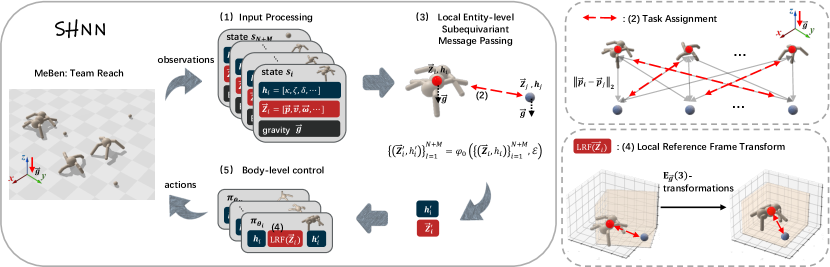
Figure 2: The flowchart of SHNN. On the left, The states of each entity $i$ are processed into scalar features ${\bm{h}}_{i}$ and directional geometric vectors $\vec{{\bm{Z}}}_{i}$, and are updated by local entity-level subequivariant message passing in a task assignment entity-level graph. Finally, the invariant local reference frame body-level control policy is obtained. Here, function $\varphi_{o}$ serves as the local entity-level subequivariant MP, and ${\mathcal{E}}$ is the local entity-level graph topology. The right side illustrates our key innovation: the dynamic task assignment leveraging bipartite graph matching, and the construction of an $\text{E}_{\vec{\bm{g}}}(3)$-equivariant local reference frame for each entity to address local transformations.

Task Assignment

In multi-entity environments, it is crucial to manage complex interactions among entities. Initially, we consider a fully connected entity-level graph ${\mathcal{G}}=({\mathcal{V}},{\mathcal{E}})$, with ${\mathcal{V}}=\Omega$ and ${\mathcal{E}}=\{(i,j):i,j\in\Omega,i\neq j\}$. To decouple local transformations from the overall structure, we introduce task assignment which dynamically adjusts the edges, forming local graphs of associated entities. The graph is then redefined as a task assignment entity-level graph, where ${\mathcal{E}}=\{(i,j):i,j\in\Omega,\mathcal{C}(i)=\mathcal{C}(j)\}$ and $\mathcal{C}$ are the assignment labels. This assignment, akin to part segmentation (Deng et al., 2023), selectively links related entities, like agents and their objects. Specifically, in this study, we employ a rule-based task assignment approach using bipartite graph matching, guided by inter-entity distance costs. Due to the static programming characteristics of JAX, implementing the Hungarian matching algorithm proves challenging. Consequently, we employ a greedy strategy-based bipartite graph matching (refer to Algorithm 1).

Local Entity-level Subequivariant Message Passing

We propose enhancing mainstream Neural Networks (such as MLPs) in RL with an additional local entity-level subequivariant message passing (MP). This task assignment entity-level graph adeptly integrates local entity-level information from related entities and, through local subequivariant MP, efficiently instills the desired local physical geometric symmetry in environments with gravity into mainstream Neural Networks to address local transformations.

For each entity $i\in\Omega$, input node features are initialized using the entity’s root state. Specifically, $\vec{{\bm{Z}}}_{i}$ is assigned as $\vec{{\bm{Z}}}_{i,1}$, and ${\bm{h}}_{i}$ is set as $[{\bm{h}}_{i,1},\vec{{\bm{p}}}_{i,1}^{z}]$, where [ ] is the stack along the last dimension and $\vec{{\bm{p}}}_{i,1}^{z}$ represents the projection of the coordinate $\vec{{\bm{p}}}_{i,1}$ onto the $z$-axis. This projection effectively indicates the relative height of entity $i$, considering the ground as the reference point.

Within the context of entity-level interactions, our function $\varphi_{o}$ serves as the local entity-level subequivariant MP. It updates each entity’s node features by considering the collective input features and the established graph connectivity.

$$\{(\vec{{\bm{Z}}}^{\prime}_{i},{\bm{h}}^{\prime}_{i})\}_{i=1}^{N+M} =\varphi_{o}\left(\{(\vec{{\bm{Z}}}_{i},{\bm{h}}_{i})\}_{i=1}^{N+M},{\mathcal{E}}\right).$$ (2)

Specifically, $\varphi_{o}$ is unfolded as the following MP and aggregation computations:

$$\vec{{\bm{Z}}}_{ij} =[(\vec{{\bm{p}}}_{j,1}-\vec{{\bm{p}}}_{i,1}),\vec{{\bm{Z}}}_{i},\vec{{\bm{Z}}}_{j}],$$ (3)

$${\bm{h}}_{ij} =[\|\vec{{\bm{p}}}_{j,1}-\vec{{\bm{p}}}_{i,1}\|_{2},{\bm{h}}_{i},{\bm{h}}_{j}],$$ (4)

$$\vec{{\bm{M}}}_{ij},{\bm{m}}_{ij} =\phi_{\vec{{\bm{g}}}}\left(\vec{{\bm{Z}}}_{ij},{\bm{h}}_{ij}\right),$$ (5)

$$\vec{{\bm{M}}}_{i},{\bm{m}}_{i} =\sum\nolimits_{j\in{\mathcal{N}}(i)}\vec{{\bm{M}}}_{ij},\sum\nolimits_{j\in{\mathcal{N}}(i)}{\bm{m}}_{ij},$$ (6)

$$(\vec{{\bm{Z}}}^{\prime}_{i},{\bm{h}}^{\prime}_{i}) =(\vec{{\bm{Z}}}_{i},{\bm{h}}_{i})$$ (7)

$$+\psi_{\vec{{\bm{g}}}}\left([\vec{{\bm{M}}}_{i},\vec{{\bm{Z}}}_{i}],[{\bm{m}}_{i},{\bm{h}}_{i}]\right),$$

where [ ] denotes the stack along the last dimension, ${\mathcal{N}}(i)=\{j:(i,j)\in{\mathcal{E}}\}$ is the neighbors of node $i$, and both $\phi_{\vec{{\bm{g}}}}$ and $\psi_{\vec{{\bm{g}}}}$ are subequivariant (Han et al., 2022; Chen et al., 2023), simplified as follows:

$$\begin{aligned} &f_{\vec{{\bm{g}}}}(\vec{{\bm{Z}}},{\bm{h}})=[\vec{{\bm{Z}}},\vec{{\bm{g}}}]{\bm{M}}_{\vec{{\bm{g}}}},\\ &\text{s.t.}\quad{\bm{M}}_{\vec{{\bm{g}}}}=\sigma([\vec{{\bm{Z}}},\vec{{\bm{g}}}]^{\top}[\vec{{\bm{Z}}},\vec{{\bm{g}}}],{\bm{h}}),\end{aligned}$$ (8)

where $\sigma\left(\cdot\right)$ is an Multi-Layer Perceptron (MLP) and $[\vec{{\bm{Z}}},\vec{{\bm{g}}}]\in{\mathbb{R}}^{3\times(m+1)}$ is a stack of $\vec{\bm{Z}}$ and $\vec{\bm{g}}$ along the last dimension. The specific form of the function is detailed in  Section C.1.

We establish a subequivariant edge representation $\vec{{\bm{Z}}}_{ij}$ and invariant edge features ${\bm{h}}_{ij}$. The edge features $\vec{{\bm{Z}}}_{ij}$ and ${\bm{h}}_{ij}$ are then input into $\phi_{\vec{{\bm{g}}}}$, as defined in  Equation 5, to yield vector and scalar messages $\vec{{\bm{M}}}_{ij}$ and ${\bm{m}}_{ij}$, respectively. Message aggregation and state updates are performed as outlined in Equation 6 and Equation 7 using the function $\psi_{\vec{{\bm{g}}}}$, leading to the updated states $\vec{{\bm{Z}}}^{\prime}_{i}$ and ${\bm{h}}^{\prime}_{i}$. This process ensures the generation of outputs maintaining the desired subequivariance or invariance properties.

Local Reference Frame Transform

Following the local entity-level subequivariant MP, we integrate the resultant entity-level information ${\bm{h}}^{\prime}_{i}$ and $\vec{{\bm{Z}}}^{\prime}_{i}$ with body-level information to guide body-level control. Here, $\vec{{\bm{u}}}_{i}$ represents a local reference frame (LRF) transform vector, derived through the linear transformation $\vec{{\bm{u}}}_{i}=\vec{{\bm{Z}}}^{\prime}_{i}{\bm{W}}_{\vec{{\bm{u}}}}$, with ${\bm{W}}_{\vec{{\bm{u}}}}\in{\mathbb{R}}^{m\times 1}$.

We normalize and orthogonalize the transform vector $\vec{{\bm{u}}}_{i}$ for each entity:

$$\vec{{\bm{e}}}_{i1} =\frac{\vec{{\bm{u}}}_{i}-\langle\vec{{\bm{u}}}_{i},\vec{{\bm{e}}}_{i3}\rangle\vec{{\bm{e}}}_{i3}}{\|\vec{{\bm{u}}}_{i}-\langle\vec{{\bm{u}}}_{i},\vec{{\bm{e}}}_{i3}\rangle\vec{{\bm{e}}}_{i3}\|},$$ (9)

$$\vec{{\bm{e}}}_{i2} =\vec{{\bm{e}}}_{i1}\times\vec{{\bm{e}}}_{i3},$$

$$\vec{{\bm{e}}}_{i3} =[0,0,1]^{\top}.$$

Here, $\langle\cdot,\cdot\rangle$ denotes the inner product, and $\times$ the cross product. We refer to the aforementioned procedure as OP, following which we proceed to construct an entity-wise rotation matrix on transform vectors.

$${\bm{O}}_{i}=\left[\vec{{\bm{e}}}_{i1},\vec{{\bm{e}}}_{i2},\vec{{\bm{e}}}_{i3}\right]=\operatorname{OP}(\vec{{\bm{u}}}_{i}),\quad i\in\Omega.$$ (10)

Theorem 3.1.

The learned entity-wise rotation matrix, denoted as ${\bm{O}}_{i}=\operatorname{OP}(\vec{{\bm{u}}}_{i})$, are $\text{SO}_{\vec{\bm{g}}}(3)$-equivariant, satisfying any transformation $g\in\text{SO}_{\vec{\bm{g}}}(3)$, $g\cdot{\bm{O}}_{i}=\operatorname{OP}(g\cdot\vec{{\bm{u}}}_{i})$.

Proof.

See Appendix A. ∎

At this stage, we establish the LRF for each agent $i$, with $\vec{{\bm{c}}}$ as the origin and $\vec{{\bm{e}}}_{i1}$ as the orientation of the $x$-axis. Notably, with the task assignment, the origin of each agent’s LRF shifts from the collective average root position $\vec{\bm{c}}=\frac{1}{N+M}\sum_{i=1}^{N+M}\vec{\bm{p}}_{i,1}$, to the specific entity’s position, $\vec{\bm{c}}=\vec{\bm{p}}_{\mathcal{C}(i),1}$. This LRF construction enables us to achieve invariant observation inputs:

$${\bm{o}}^{\prime}_{i}={\bm{O}}_{i}^{\top}{\bm{o}}_{i}=[\{{\bm{O}}_{i}^{\top}\vec{{\bm{Z}}}_{i,k},{\bm{h}}_{i,k}\}_{k=1}^{K_{i}},{\bm{O}}_{i}^{\top}\vec{{\bm{Z}}}_{j,1},{\bm{h}}_{j,1}],$$ (11)

where $j\in{\mathcal{N}}(i)$, and [ ] is the stack along the last dimension, with adjustments for relative positioning in assignment as $\vec{\bm{p}}_{i,k}=\vec{\bm{p}}_{i,k}-\vec{\bm{p}}_{\mathcal{C}(i),1},\vec{\bm{p}}_{j,1}=\vec{\bm{p}}_{j,1}-\vec{\bm{p}}_{\mathcal{C}(j),1}$, thus achieving decoupled translation and rotation invariance.

Our methodology integrates subequivariant information across entity and body levels via LRF Transform. While disrupting reflection symmetry, the necessity to construct an orthogonal rotation matrix significantly enhances the capabilities of subequivariant networks. This emphasis on rotation symmetry substantially outweighs the reduced focus on reflection symmetry, particularly in diminishing the massive search space for optimal policies. Empirical validations of this enhancement are detailed in Section 5.4.

Body-level Control

We are now equipped to output the invariant actor policy $\pi_{\theta}$ and invariant critic value-function $V_{\phi}$ for the training objective in Equation 1. For each agent $i$, the invariant actor policy $\pi_{\theta_{i}}$ leverages the invariant ${\bm{o}}^{\prime}_{i}$ and ${\bm{h}}^{\prime}_{i}$, defined by

$$\pi_{\theta_{i}}=\sigma_{\pi_{i}}({\bm{o}}^{\prime}_{i},{\bm{h}}^{\prime}_{i}),$$ (12)

where $\sigma_{\pi_{i}}$ is a MLP. Here, $\pi_{\theta_{i}}\in{\mathbb{R}}^{2\times(K_{i}-1)}$ represents the loc and scale parameters of a Tanh-Normal Distribution for the $(K_{i}-1)$ actuators of agent $i$. Consequently, each actuator samples its corresponding torque $a_{i,k}\in[-1,1]$ from this distribution.

Besides, the invariant critic value-function $V_{\phi}$ utilizes the entity-level invariant features $\{{\bm{h}}^{\prime}_{i}\}_{i=1}^{N+M}$, formulated as

$$V_{\phi}=\sigma_{V}(\{{\bm{h}}^{\prime}_{i}\}_{i=1}^{N+M}),$$ (13)

where $\sigma_{V}$ is a MLP, and $V_{\phi}\in{\mathbb{R}}$. Formal proof of the $\text{SO}_{\vec{\bm{g}}}(3)$-invariance of the output action and value are presented in Appendix A.

4 Multi-entity Benchmark (MeBen)

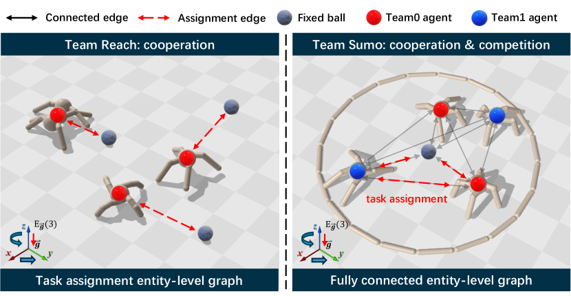
Figure 3: Illustration of MeBen: Team Reach (left) where agents cooperate to collectively reach all fixed balls, and Team Sumo (right) where agents engage in both cooperation and competition to push opponents away from the fixed ball. These tasks necessitate the decoupling of local transformations via dynamic task assignment graph construction from the overall structure (depicted by a fully connected graph), while employing $\text{E}_{\vec{\bm{g}}}(3)$-equivariance to effectively compress global state space.

4.1 Environments descriptions

In this subsection, we present the details involved in constructing our environments: Team Reach and Team Sumo, as illustrated in Figure 3.

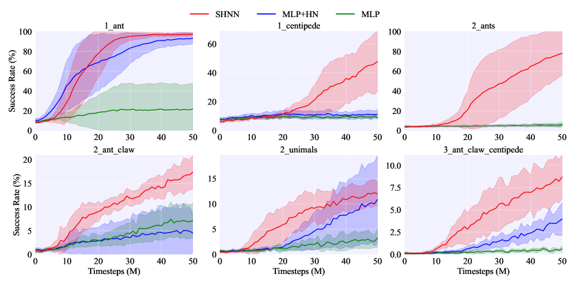
Figure 4: Training and Evaluation Curves in Team Reach Environments. The shaded area represents the standard error.

Agents

In our studies, we leverage a variety of morphologies, including ants, claws, and centipedes from MxT-Bench (Furuta et al., 2023), as well as unimals from Gupta et al. (2022). Notably, centipedes and unimals exhibit asymmetrical forms, potentially influencing the overall system’s symmetry and dynamics. This diverse range of agent morphologies enables a nuanced exploration of agent dynamics in multi-entity, morphology-based RL environments.

Team Reach

We expand the “Reach” task from a single-agent challenge to a collaborative “Team Reach” task, as shown in Figure 9. 1. Initial Conditions. Entities set $\Omega$ include $N$ agents and $M$ fixed balls, $N\geq M$. Within an area of radius $R$, we randomly position $N$ agents and $M$ fixed balls, also setting the initial orientations of the agents randomly. Specific details for $N$, $M$, $R$, and the agents’ morphology are provided in Table 4. 2. Termination. The goal of this task is for $M$ fixed balls to be simultaneously occupied by agents. An episode is considered successfully completed and terminates once this condition is fulfilled. 3. Reward. The designed reward is detailed in Section C.2.

Team Sumo

We evolve the “Sumo” task from a purely competitive challenge to a mixed cooperative-competitive “Team Sumo” task, as shown in Figure 10. 1. Initial Conditions. Entities set $\Omega$ comprise one fixed ball, $N$ agents forming Team 1, and another $M$ agents constituting Team 2. The sumo arena, a circle with radius $R$, has its center marked by the fixed ball. Around this fixed ball, within a radius of $R-1$, we randomly position $N$ agents from Team 1 and another $M$ from Team 2, ensuring each agent’s orientation is also randomized. Specific details for $N$, $M$, $R$, and the agents’ morphology are provided in Table 4. 2. Termination. The objective is for either Team 1 or Team 2 to win by having an opposing team’s agent disqualified, which occurs if it exceeds a distance $R$ from the fixed ball. The team with the disqualified agent loses, triggering the termination of the episode. 3. Reward. The reward designed for each team is detailed in Section C.2.

Table 1: Comparison of Morphology-based Environment Setup.

Aspect	SGRL	MxT-Bench	MeBen
Multi-Morphology	✓	✓	✓
Multi-Agent	×	×	✓
Diverse-Task	×	✓	✓
Supported-Symmetry	✓	×	✓
Accelerated-Hardware	×	✓	✓

4.2 Design considerations

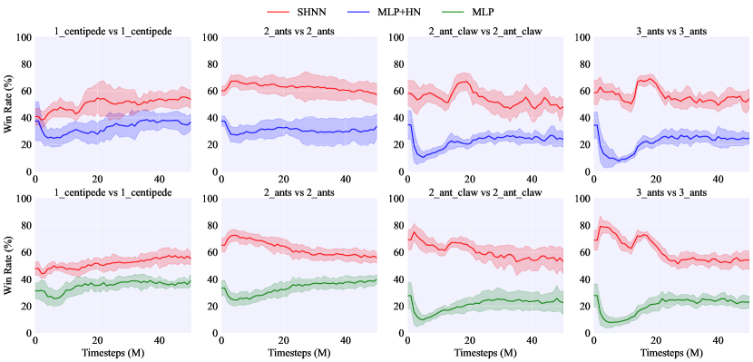
Figure 5: Training and Evaluation Curves in Team Sumo Environments. The shaded area represents the standard error.

We present the key features and limitations of existing benchmarks in Table 1, comparing them with our introduced MeBen. More comprehensive details are provided below.

Multi-Entity Dynamics

Diverging from the single-agent focus in SGRL (Chen et al., 2023) and MxT-bench (Furuta et al., 2023), MeBen expands to include environments with multiple entities (Spelke, 2022), enabling a detailed exploration of dynamics and interactions among varied entities, such as agents with complex morphologies, and other significant objects impacting system symmetry and behavior. MeBen’s unique design, makes it an ideal platform for a wide range of morphology-based reinforcement learning studies, encompassing single-agent and multi-agent systems (cooperative, competitive, and mixed scenarios).

Geometric Symmetry

In contrast to the fixed agent initialization in MxT-bench (Furuta et al., 2023), MeBen provides a more realistic and geometric symmetric setup through its stochastic initial conditions. The positions and orientations of all entities, including agents and objects, are uniformly randomized in MeBen’s environments. This strategy eliminates any bias towards specific orientations or positions, maintaining geometric symmetry and providing a robust test bed for evaluating the generalization capabilities of models in environments with gravity.

Accelerated-Hardware

In contrast to traditional CPU-based environments such as SGRL (Chen et al., 2023), MeBen harnesses the advanced capabilities of the Brax physics simulator (Freeman et al., 2021) and Composer (Gu et al., 2021), and further builds upon the MxT-bench framework (Furuta et al., 2023). This advancement propels MeBen into facilitating efficient and scalable hardware-accelerated iterations on GPUs or TPUs, making it exceptionally suitable for morphology-based reinforcement learning experiments.

Table 2: Evaluations on Basic Architectures. Training and Evaluation in Team Reach Environments. We report Success Rate (%) on the final step.

Methods	1_ant	1_centipede	2_ants	2_ant_claw	2_unimals	2_ant_claw_centipede
MLP+HN	93.39 $\pm$ 5.25	11.28 $\pm$ 3.21	5.25 $\pm$ 1.399	4.52 $\pm$ 3.93	10.86 $\pm$ 8.74	3.98 $\pm$ 1.83
SHNN	97.26 $\pm$ 1.51	47.82 $\pm$ 20.62	77.93 $\pm$ 22.22	17.40 $\pm$ 3.54	11.97 $\pm$ 2.31	8.70 $\pm$ 2.42
Transformer+HN	5.47 $\pm$ 2.84	5.55 $\pm$ 2.99	2.47 $\pm$ 0.73	0.51 $\pm$ 0.19	0.25 $\pm$ 0.10	2.26 $\pm$ 1.92
SHTransformer	63.61 $\pm$ 39.57	11.52 $\pm$ 2.39	11.37 $\pm$ 15.50	1.17 $\pm$ 0.70	0.26 $\pm$ 0.15	7.12 $\pm$ 2.29

5 Experiments

5.1 Experimental Setup

Baselines

We compare our method SHNN, against mainstream neural networks, particularly MLP  (Furuta et al., 2023), and its variant utilizing heading normalization tricks, denoted as MLP+HN (Chen et al., 2023). Please refer to Section C.3 for details about baselines.

Metrics

1. Team Reach: Success Rate = #success_episode / #evaluation_episode. 2. Team Sumo: For each team, Win Rate = #win_episode / #evaluation_episode. Each experiment is conducted with 10 seeds to report the Success (or Win) Rate over #evaluation_episode of $1024$.

Implementations

The environments used in this work are detailed in Table 4. To ensure fairness, all baselines, ablations, and our SHNN model use the same input information and employ MAPPO (Yu et al., 2022) as the training algorithm for MARL. SHNN is developed based on the MxT-bench(Furuta et al., 2023) codebase, leveraging JAX(Bradbury et al., 2018) and Brax (Freeman et al., 2021; Gu et al., 2021) for efficient, hardware-accelerated simulations. The value of the maximum timesteps per episode is $1000$. Hyperparameter details are in Section C.9. Within the same team, agents share only the weights of entity-level message passing, not the body-level MLP. For the Team Reach environments, we construct a directed graph by dynamically assigning a fixed ball to each agent. For the Team Sumo environments, we assign each agent an opponent from the opposing team and assign each with the arena’s center ball. Additionally, in Team Sumo environments, we adopt Bansal et al. (2018)’s approach where teams employing baseline methods and SHNN compete within an arena.

5.2 Evaluations in Diverse Environments

We begin by evaluating our method on diverse multi-entity tasks in 3D environments. Team Reach in Figure 4: 1. The MLP generally fails to achieve meaningful returns in most Team Reach cases, which is due to its vulnerability to local extremes within the expansive exploration space of our environments. 2. While MLP enhanced with Heading Normalization (MLP+HN) shows close performance to SHNN in specific environments like 1_ant and 2_unimals, their effectiveness diminishes in other scenarios. This variation in performance can be attributed to factors such as the symmetry in morphology and the complexities arising from multi-agent interactions. 3. Our proposed SHNN demonstrates a clear advantage, outperforming all baselines across various scenarios. Team Sumo in Figure 5: with an increase in the number and complexity of agent morphologies, the advantage of our method over baselines progressively amplifies. These observations underscore that our proposed SHNN method not only exhibits superior capabilities in compressing the global state space of multi-entity tasks and significantly enhances the generalization of body-level policies, but also sees these advantages magnified in scenarios with increasingly complex agent morphologies and a greater number of agents.

5.3 Extended Evaluations on Transformer

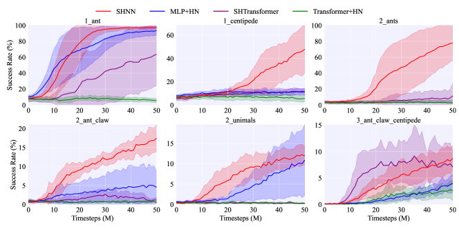
Figure 14: Evaluations on Transformer Architecture. Training and Evaluation Curves in Team Reach Environments.

Additionally, building upon our initial exploration with MLP, our exploration extended to Transformers, utilizing the same backbone as Amorpheus (Kurin et al., 2020) and MxT-Bench (Furuta et al., 2023) for $\sigma_{\pi_{i}}$ in Equation 12 and $\sigma_{V}$ in Equation 13. Despite Transformers’ advances in morphology-based RL (Kurin et al., 2020; Hong et al., 2021; Dong et al., 2022; Chen et al., 2023; Furuta et al., 2023), their training complexity and computational demands limit their performance improvement over MLPs in environments with restricted agent morphology diversity, as detailed in Table 5 and Table 2, with curves in Figure 14. Moreover, SHTransformer (our plug-in applied to body-level Transformer control) consistently outperforms standard Transformer models. This evidence confirms the plug-in’s broad applicability and effectiveness across varied architectural frameworks.

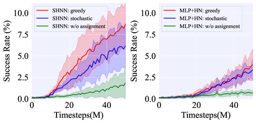
Figure 6: Ablations on Assignment. Training and Evaluation Curves in 3_ant_claw_centipede Team Reach.

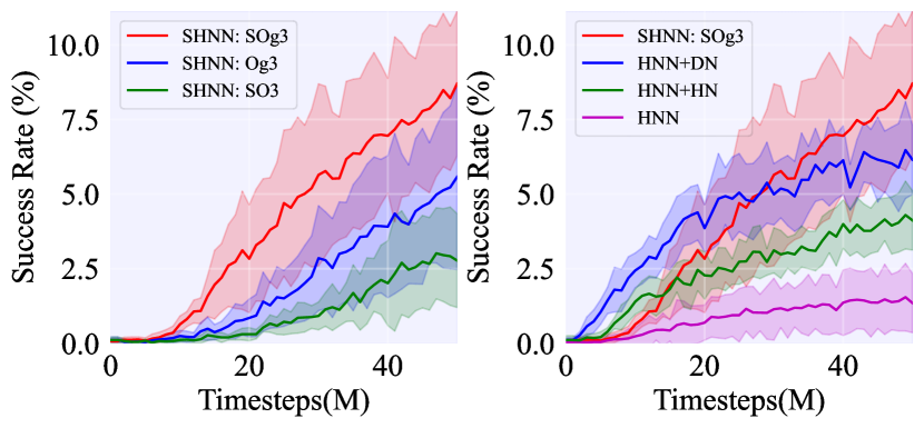
Figure 7: Ablations on Equivariance. Training and Evaluation Curves in 3_ant_claw_centipede Team Reach.

5.4 Ablation Studies

Ablations on Assignment

We evaluate the impact of task assignment by comparing several variants, as depicted in Figure 6 and Figure 11. We consider the following configurations: greedy, a default model that employs a greedy strategy-based bipartite matching for task assignment; stochastic, a variant based on stochastic assignments; w/o assignment, a variant where no task assignment is performed, with the entity-level graph configured as a fully connected graph and sparse root mean $\vec{\bm{c}}=\frac{1}{N+M}\sum_{i=1}^{N+M}\vec{\bm{p}}_{i,1}$ serving as the origin of LRF in  Equation 11. Our empirical findings affirm that assignment consistently enhances performance across various neural networks architectures in the Team Reach environments. Specifically, MLP networks exhibit marked improvement when incorporating task assignments. For SHNN, the greedy graph matching strategy of task assignment significantly outperforms both stochastic and non-assignment strategies. This evidence underscores that our task assignment effectively facilitates task-specific dynamics, managing complex entity interactions by decoupling local transformations from the overall structures while compressing the search space through local physical symmetry. For Team Sumo, see Section C.5.

Ablations on Equivariance

We ablate the following variants in Figure 7 and Figure 12: SHNN:SOg3, our full model, which is $\text{SO}_{\vec{{\bm{g}}}}(3)$-equivariant; SHNN:Og3, an $\text{O}_{\vec{{\bm{g}}}}(3)$-equivariant variant, where ${\bm{O}}_{i}=\vec{{\bm{Z}}}^{\prime}_{i}$ in Equation 10; SHNN:SO3, a $\text{SO}(3)$-equivariant variant, where $\vec{\bm{g}}$ is omitted in the computation in Equation 8; HNN+DN, a non-equivariant variant, where $\vec{{\bm{Z}}}$ are treated as scalars, but which utilizes the goal direction to construct the LRF; HNN+HN, a non-equivariant variant, where $\vec{{\bm{Z}}}$ are treated as scalars, but which utilizes the agent’s heading direction to construct the LRF; HNN, a non-equivariant variant, where $\vec{{\bm{Z}}}$ are treated as scalars. 1. Which symmetry group works best within our network framework? Comparative experiments between the $\text{SO}_{\vec{{\bm{g}}}}(3)$ group and the $\text{O}_{\vec{{\bm{g}}}}(3)$ group show that the positive impact of emphasizing rotational symmetry significantly outweighs any disadvantages from the reduced focus on reflection symmetry, particularly in terms of reducing the massive search space. Furthermore, the comparison between the $\text{SO}_{\vec{{\bm{g}}}}(3)$ group and the $\text{SO}(3)$ group demonstrates the importance of sensing the direction of gravity in policy learning. 2. Can equivariant network methods replace or even surpass methods based on hand-crafted LRF? Experiments demonstrate that whether using goal orientation or the agent’s heading orientation to construct the LRF, the performance is inferior compared to ours. This indicates that for current mainstream neural networks, entity-level subequivariant message passing emerges as a simpler yet more effective alternative to hand-crafted LRF, providing a plug-in solution for equivariant modifications.

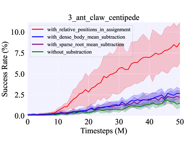
Figure 8: Local Translation Invariance. Training and Evaluation Curves in 3_ant_claw_centipede Team Reach Environment.

Importance of Local Symmetry

The analysis of local symmetry in the Team Reach environments, illustrated by comparing the red and green lines in the left plot of Figure 6, and the red and purple lines in the right plot of Figure 7, underscores the indispensable roles of task assignment and equivariance. Their integration is pivotal for surmounting the benchmark’s challenges, validating the SHNN method’s design philosophy. To further substantiate the criticality of local symmetry, we embarked on ablation studies exploring the influence of local translation invariance with the following variants: without subtraction, where no translation invariance implemented; with sparse root mean subtraction: $\vec{\bm{c}}=\frac{1}{N+M}\sum_{i=1}^{N+M}\vec{\bm{p}}_{i,1}$, i.e., without decoupling translation transformations; with dense body mean subtraction, $\vec{\bm{c}}=\frac{1}{\sum_{i=1}^{N+M}\sum_{k=1}^{K_{i}}1}\sum_{i=1}^{N+M}\sum_{k=1}^{K_{i}}\vec{\bm{p}}_{i,k}$, i.e., without decoupling translation transformations; with relative positions in assignment, $\vec{\bm{c}}=\vec{\bm{p}}_{\mathcal{C}(i),1}$, i.e., with decoupling of translation transformations. The results in Figure 8 clearly indicate that without achieving translation invariance or properly decoupling it, the model struggles to mitigate complexity challenges, leading to significantly poorer performance. This observation further emphasizes the pivotal importance of local symmetry.

5.5 Analyses of Morphology-shared Policy

Table 3: Analyses of Morphology-shared Policy. We report Success Rate (%) on the final step in Team Reach Environments.

Methods	2_ants	3_ant_claw_centipede
SHNN	$\textbf{77.93}\pm 22.22$	$8.70\pm 2.42$
SHGNN	$41.41\pm 29.47$	$\textbf{31.07}\pm 26.84$

Previous works have achieved generalization across agents with different morphologies using morphology-aware Graph Neural Networks (Wang et al., 2018; Huang et al., 2020). In addition to the previously mentioned SHTransformer (our plug-in applied to body-level Transformer control), we have also developed a new variant, denoted as SHGNN (our plug-in applied to body-level message passing control). This variant learns a shared policy network across different agents, detailed in Section C.6. As observed in Table 3 and Table 5, despite body-level message passing excelling in complex, multi-morphological environments by enhancing knowledge sharing and performance, its implementation significantly slows down the training process. Above all, our benchmark provides the community with a test bed that takes into account both agent-interaction and morphology-aware considerations.

6 Limitations and Future Works

To learn policies in 3D multi-entity physical environments, we propose the SHNN, a framework that uniquely integrates task assignment with local subequivariant message passing in a hierarchical structure. However, in the Team Sumo environments, as shown in Figure 11, the impact of assignment is not as significant as that of equivariance. Therefore, the interdependence of task assignment and equivariance necessitates a novel co-learnable formulation. Our model’s reliance on the $\text{E}_{\vec{\bm{g}}}(3)$ symmetry encompasses a broad range of physical interactions but does not extend to non-Euclidean or highly irregular environments not governed by classical physics. Additionally, our model predominantly leverages state-based inputs, which are often costly to acquire in practice due to the need for precision sensors. Addressing the challenge of applying our equivariance-focused approach to vision-based inputs remains an open area for future research.

Impact Statement

The research presented in this paper is a step toward advancing the field machine learning (Yin et al., 2024; Guan et al., 2024). While our contributions focus on the theoretical and technical advancements in machine learning, we acknowledge the broader societal implications as our work indirectly supports the development of technologies in delivery, transportation, and automated systems. The practical applications, such as in autonomous vehicles and drones, offer promising avenues for societal benefits, including improved safety and efficiency. While our work heralds technical progress, we are mindful of its societal impacts, notably privacy concerns from using detailed state data, emphasizing the need for robust policies to ensure these technologies’ ethical and secure societal integration.

Appendix A Proofs

In this section, we theoretically prove that our proposed SHNN ensures the final output action and critic value preserve the symmetry as desired.

Theorem A.1.

The learned entity-wise rotation matrix, denoted as ${\bm{O}}_{i}=\operatorname{OP}(\vec{{\bm{u}}}_{i})$, are $\text{SO}_{\vec{{\bm{g}}}}(3)$-equivariant, satisfying any transformation $g\in\text{SO}_{\vec{{\bm{g}}}}(3)$, $g\cdot{\bm{O}}_{i}=\operatorname{OP}(g\cdot\vec{{\bm{u}}}_{i})$.

Proof.

To prove that the entity-wise rotation matrix ${\bm{O}}_{i}=\operatorname{OP}(\vec{{\bm{u}}}_{i})$ are $\text{SO}_{\vec{{\bm{g}}}}(3)$-equivariant, we need to show that under any transformation $g\in\text{SO}_{\vec{{\bm{g}}}}(3)$, the transformation of ${\bm{O}}_{i}$ through $g$ is equivariant to the rotation matrix obtained from the transformed vectors $g\cdot\vec{{\bm{u}}}_{i}$.

Let $g$ be a transformation in $\text{SO}_{\vec{{\bm{g}}}}(3)$, which includes a rotation ${\bm{O}}$ along the direction of $\vec{\bm{g}}$. Specifically, the transformation is applied as follows:

$$g\cdot{\bm{O}}_{i} ={\bm{O}}{\bm{O}}_{i},$$

$$g\cdot\vec{{\bm{u}}}_{i} ={\bm{O}}\vec{{\bm{u}}}_{i},$$

Let ${\bm{O}}_{i}^{\ast}=\operatorname{OP}(g\cdot\vec{{\bm{u}}}_{i})$. By the properties of the orthogonalization process, we have:

$$\vec{{\bm{e}}}_{i1}^{\ast} =\frac{{\bm{O}}\vec{{\bm{u}}}_{i}-\langle{\bm{O}}\vec{{\bm{u}}}_{i},\vec{{\bm{e}}}_{i3}^{\ast}\rangle\vec{{\bm{e}}}_{i3}^{\ast}}{\|{\bm{O}}\vec{{\bm{u}}}_{i}-\langle{\bm{O}}\vec{{\bm{u}}}_{i},\vec{{\bm{e}}}_{i3}^{\ast}\rangle\vec{{\bm{e}}}_{i3}^{\ast}\|},$$

$$\vec{{\bm{e}}}_{i2}^{\ast} =\vec{{\bm{e}}}_{i1}^{\ast}\times\vec{{\bm{e}}}_{i3}^{\ast},$$

$$\vec{{\bm{e}}}_{i3}^{\ast} =[0,0,1]^{\top}.$$

Since ${\bm{O}}\vec{\bm{g}}=\vec{\bm{g}}$, ${\bm{O}}^{\top}{\bm{O}}={\bm{I}}$ and $\det({\bm{O}})=1$, it preserves inner products and norms. And, the cross product obeys the following identity under matrix transformations: $(M\vec{{\bm{a}}})\times(M\vec{{\bm{b}}})=(\operatorname{det}M)\left(M^{-1}\right)^{\mathrm{T}}(\vec{{\bm{a}}}\times\vec{{\bm{b}}})$. Therefore, $\vec{{\bm{e}}}_{i3}^{\ast}={\bm{O}}\vec{{\bm{e}}}_{i3}$, $\|{\bm{O}}\vec{{\bm{u}}}_{i}\|=\|\vec{{\bm{u}}}_{i}\|$ and $\langle{\bm{O}}\vec{{\bm{u}}}_{i},{\bm{O}}\vec{{\bm{e}}}_{i3}\rangle=\langle\vec{{\bm{u}}}_{i},\vec{{\bm{e}}}_{i3}\rangle$. This implies:

$$\vec{{\bm{e}}}_{i1}^{\ast} =\frac{{\bm{O}}\vec{{\bm{u}}}_{i}-\langle{\bm{O}}\vec{{\bm{u}}}_{i},{\bm{O}}\vec{{\bm{e}}}_{i3}\rangle{\bm{O}}\vec{{\bm{e}}}_{i3}}{\|{\bm{O}}\vec{{\bm{u}}}_{i}-\langle{\bm{O}}\vec{{\bm{u}}}_{i},{\bm{O}}\vec{{\bm{e}}}_{i3}\rangle{\bm{O}}\vec{{\bm{e}}}_{i3}\|}=\frac{{\bm{O}}\vec{{\bm{u}}}_{i}-\langle\vec{{\bm{u}}}_{i},\vec{{\bm{e}}}_{i3}\rangle{\bm{O}}\vec{{\bm{e}}}_{i3}}{\|{\bm{O}}\vec{{\bm{u}}}_{i}-\langle\vec{{\bm{u}}}_{i},\vec{{\bm{e}}}_{i3}\rangle{\bm{O}}\vec{{\bm{e}}}_{i3}\|}=\frac{{\bm{O}}(\vec{{\bm{u}}}_{i}-\langle\vec{{\bm{u}}}_{i},\vec{{\bm{e}}}_{i3}\rangle\vec{{\bm{e}}}_{i3})}{\|\vec{{\bm{u}}}_{i}-\langle\vec{{\bm{u}}}_{i},\vec{{\bm{e}}}_{i3}\rangle\vec{{\bm{e}}}_{i3}\|}={\bm{O}}\vec{{\bm{e}}}_{i1},$$

$$\vec{{\bm{e}}}_{i2}^{\ast} ={\bm{O}}\vec{{\bm{e}}}_{i1}\times{\bm{O}}\vec{{\bm{e}}}_{i3}=\det({\bm{O}}){\bm{O}}(\vec{{\bm{e}}}_{i1}\times\vec{{\bm{e}}}_{i3})={\bm{O}}\vec{{\bm{e}}}_{i3},$$

$$\vec{{\bm{e}}}_{i3}^{\ast} =[0,0,1]^{\top}={\bm{O}}\vec{{\bm{e}}}_{i3}.$$

Therefore, with ${\bm{O}}_{i}^{\ast}=\operatorname{OP}(g\cdot\vec{{\bm{u}}}_{i})=\left[{\bm{O}}\vec{{\bm{e}}}_{i1},{\bm{O}}\vec{{\bm{e}}}_{i2},{\bm{O}}\vec{{\bm{e}}}_{i3}\right]={\bm{O}}{\bm{O}}_{i}=g\cdot{\bm{O}}_{i}$, we confirm the $\text{SO}_{\vec{{\bm{g}}}}(3)$-equivariance of ${\bm{O}}_{i}$.

Besides, for reflection transformations ${\bm{O}}$, characterized by ${\bm{O}}^{\top}{\bm{O}}={\bm{I}}$ and $\det({\bm{O}})=-1$, $\vec{{\bm{e}}}_{i2}^{\ast}=-{\bm{O}}\vec{{\bm{e}}}_{i2}\rightarrow{\bm{O}}_{i}^{\ast}\neq{\bm{O}}{\bm{O}}_{i}$ where the equivariance is disrupted due to the properties of the cross product. Hence, although we utilize an $\text{O}_{\vec{{\bm{g}}}}(3)$-equivariant message passing network in Equation 8, the orthogonalization process can transform a $\text{O}_{\vec{{\bm{g}}}}(3)$-equivariant vector into a $\text{SO}_{\vec{{\bm{g}}}}(3)$-equivariant matrix. ∎

As for the actor and critic, we additionally have the following corollary.

Corollary A.2.

Let $\pi_{\theta_{i}},V_{\phi}$ be output of the actor and the critic of SHNN with $\vec{\bm{Z}},\vec{\bm{g}},{\bm{h}}$ as input. Let $\pi_{\theta_{i}}^{\ast},V_{\phi}^{\ast}$ be the actor and critic with ${\bm{O}}\vec{\bm{Z}},{\bm{O}}\vec{\bm{g}},{\bm{h}}$ as input, ${\bm{O}}\in\text{SO}_{\vec{\bm{g}}}(3)$. Then, $(\pi_{\theta_{i}}^{\ast},V_{\phi}^{\ast})=(\pi_{\theta_{i}},V_{\phi})$, indicating the output actor and critic preserve $\text{SO}_{\vec{\bm{g}}}(3)$-invariance.

Proof.

Given the subequivariance of Equation 8 as per  (Han et al., 2022; Chen et al., 2023), we have ${{\bm{h}}^{\prime}_{i}}^{\ast}={\bm{h}}^{\prime}_{i}$.

Hence,

$$V_{\phi}^{\ast} =\sigma_{V}(\{{{\bm{h}}^{\prime}_{i}}^{\ast}\}_{i=1}^{N+M})$$ (14)

$$=\sigma_{V}(\{{\bm{h}}^{\prime}_{i}\}_{i=1}^{N+M})$$ (15)

$$=V_{\phi}.$$ (16)

Then, we get ${\bm{o}}_{i}^{\ast}$ with ${\bm{O}}\vec{\bm{Z}},{\bm{O}}\vec{\bm{g}},{\bm{h}}$ as input:

$${\bm{o}}_{i}^{\ast} =[\{{\bm{O}}\vec{{\bm{Z}}}_{i,k},{\bm{h}}_{i,k}\}_{k=1}^{K_{i}},{\bm{O}}\vec{{\bm{Z}}}_{j,1},{\bm{h}}_{j,1}].$$ (17)

By Theorem A.1, we can obtain ${\bm{O}}_{i}^{\ast}={\bm{O}}{\bm{O}}_{i}$ with ${\bm{O}}\vec{\bm{Z}},{\bm{O}}\vec{\bm{g}},{\bm{h}}$ as input.

Therefore, the LRF invariant observation inputs ${{\bm{o}}^{\prime}_{i}}^{\ast}$ with ${\bm{O}}\vec{\bm{Z}},{\bm{O}}\vec{\bm{g}},{\bm{h}}$ as input:

$${{\bm{o}}^{\prime}_{i}}^{\ast} ={{\bm{O}}_{i}^{\ast}}^{\top}{\bm{o}}_{i}^{\ast}$$ (18)

$$=[\{{{\bm{O}}_{i}^{\ast}}^{\top}{\bm{O}}\vec{{\bm{Z}}}_{i,k},{\bm{h}}_{i,k}\}_{k=1}^{K_{i}},{{\bm{O}}_{i}^{\ast}}^{\top}{\bm{O}}\vec{{\bm{Z}}}_{j,1},{\bm{h}}_{j,1}]$$ (19)

$$=[\{{\bm{O}}_{i}^{\top}{\bm{O}}^{\top}{\bm{O}}\vec{{\bm{Z}}}_{i,k},{\bm{h}}_{i,k}\}_{k=1}^{K_{i}},{\bm{O}}_{i}^{\top}{\bm{O}}^{\top}{\bm{O}}\vec{{\bm{Z}}}_{j,1},{\bm{h}}_{j,1}]$$ (20)

$$=[\{{\bm{O}}_{i}^{\top}\vec{{\bm{Z}}}_{i,k},{\bm{h}}_{i,k}\}_{k=1}^{K_{i}},{\bm{O}}_{i}^{\top}\vec{{\bm{Z}}}_{j,1},{\bm{h}}_{j,1}]$$ (21)

$$={\bm{O}}_{i}^{\top}{\bm{o}}_{i}={\bm{o}}^{\prime}_{i}.$$ (22)

Hence,

$$\pi_{\theta_{i}}^{\ast} =\sigma_{\pi_{i}}({{\bm{o}}^{\prime}_{i}}^{\ast},{{\bm{h}}^{\prime}_{i}}^{\ast})$$ (23)

$$=\sigma_{\pi_{i}}({\bm{o}}^{\prime}_{i},{\bm{h}}^{\prime}_{i})$$ (24)

$$=\pi_{\theta_{i}}.$$ (25)

∎

Appendix B Related Works

Morphology-based RL

In the field of reinforcement learning (RL), recent years have witnessed the emergence and evolution of morphology-based approaches, particularly within the context of inhomogeneous morphology settings. This setting is distinguished by varying state and action spaces across different tasks (Devin et al., 2017; Chen et al., 2018; D’Eramo et al., 2020). Morphology-based RL decentralizes the control of multi-joint robots by learning a shared policy for each joint, applying a multitude of message-passing strategies. To tackle the challenges of the inhomogeneous setting, methods such as NerveNet (Wang et al., 2018), DGN (Pathak et al., 2019), and SMP (Huang et al., 2020) represent the agent’s morphology as a graph and implement Graph Neural Networks (GNNs) for their policy networks. On the other hand, Amorpheus (Kurin et al., 2020), SWAT (Hong et al., 2021), ModuMorph (Xiong et al., 2023), SGRL (Chen et al., 2023), and Solar (Dong et al., 2022) opt for transformers over GNNs for direct communication. Both approaches demonstrate that graph-based policies offer significant benefits compared to conventional monolithic policies. Furthermore, MxT-Bench (Furuta et al., 2023) serves as a testbed for morphology-task generalization, though its primary focus remains on single-agent tasks. Our work, however, expands upon these methodologies to encompass multi-entity environments, facilitating comprehensive exploration of dynamics and interactions among a variety of entities, including agents with intricate morphologies, objects, and other crucial factors affecting system symmetry and behaviors.

Multi-Agent RL

In the realm of Multi-Agent RL (MARL), decision-making is predominantly guided by frameworks such as the decentralized partially observable Markov decision process (Dec-POMDP) (Bernstein et al., 2002; Oliehoek et al., 2016; Lechner et al., 2023), with strategies typically categorized into cooperative (Xu et al., 2023; Rashid et al., 2018), competitive (Bansal et al., 2018), and mixed interactions (Lowe et al., 2017). Addressing challenges like high-dimensional action spaces and the necessity for agent coordination, decentralized learning (Littman, 1994; Foerster et al., 2016) aims to independently optimize each agent’s policy. While scalable, this approach often struggles with issues of instability, especially under conditions of partial observability. On the other hand, centralized learning (Claus & Boutilier, 1998; Kraemer & Banerjee, 2016) offers a more comprehensive view but faces computational hurdles in complex environments. The Centralized Training with Decentralized Execution (CTDE) paradigm (Lowe et al., 2017; Sunehag et al., 2018; Rashid et al., 2018; Foerster et al., 2018; Iqbal & Sha, 2019; Kuba et al., 2021; Wen et al., 2022; Yu et al., 2022; Jeon et al., 2022) emerges as a balanced solution to these extremes. It allows agents to make decisions based on local observations, while global state information is utilized in the construction of the value function. This synergy of individual autonomy and collective insight enhances the efficacy of the decision-making process. Notably, Yu et al. (2022) revisited the application of Proximal Policy Optimization (PPO) in MARL within the CTDE structure, achieving remarkably strong performance. Moreover, existing multi-agent reinforcement learning (MARL) environments (Samvelyan et al., 2019; de Witt et al., 2020; Ellis et al., 2022; Rutherford et al., 2023; Lechner et al., 2023) often lack scenarios that encompass both geometric symmetry and morphology-based control. We expand existing environments (Chen et al., 2023; Furuta et al., 2023) into a suite of new multi-entity benchmark (MeBen) in 3D space, not only facilitating a comprehensive exploration of multi-entity dynamics but also ensuring a realistic emulation of real-world scenarios through randomized initial conditions and orientations. Our work aligns with the Dec-POMDP framework and capitalizes on the strengths of MAPPO (Yu et al., 2022) to optimize policies effectively. Furthermore, our environment is implemented using JAX (Bradbury et al., 2018), ensuring efficient simulations on advanced hardware accelerators such as GPUs and TPUs.

Geometrically Equivariant Models

The physical world exhibits specific symmetries, extensively explored in studies on group equivariant models (Cohen & Welling, 2016, 2017; Worrall et al., 2017). Building upon this, the field of geometrically equivariant graph neural networks (Han et al., 2024) has emerged, utilizing symmetry as a fundamental bias in learning. These models are designed to ensure that outputs will rotate, translate, or reflect in the same manner as their inputs, thereby retaining inherent symmetries. Techniques such as group convolution via irreducible representation (Thomas et al., 2018; Fuchs et al., 2020) and invariant scalarization methods, like inner product computation (Villar et al., 2021; Satorras et al., 2021; Huang et al., 2022; Han et al., 2022), are employed to achieve this symmetry preservation. Our method, similar to GMN (Huang et al., 2022) and SGNN (Han et al., 2022), especially focuses on scalarization strategies. In Markov decision processes (MDPs) that exhibit symmetries (van der Pol et al., 2020), these symmetries in the state-action space enable the optimization of policies within a simplified abstract MDP. The work of van der Pol et al. (2020) concentrates on learning equivariant policies and invariant value networks in 2D environments. In contrast, Chen et al. (2023) explores body-level equivariant policy networks in more complex 3D physics environments, facilitating policy generalization across different directions. Our work diverges by introducing an entity-level subequivariant message-passing mechanism, which proves to be highly effective in 3D multi-body scenes (Han et al., 2022).

Appendix C More Experimental Details

C.1 Subequivariant Function

We resort to subequivariant function with $\vec{\bm{Z}},\vec{\bm{g}},{\bm{h}}$ as input (Han et al., 2022; Chen et al., 2023) to instill desired geometric symmetry into the model:

$$\begin{aligned} &\vec{{\bm{Z}}}^{\prime},{\bm{h}}^{\prime}=\vec{{\bm{M}}}_{\vec{{\bm{g}}}}{\bm{W}}_{\vec{{\bm{g}}}},{\bm{W}}_{\vec{{\bm{g}}}},\\ &\text{s.t.}\quad{\bm{W}}_{\vec{{\bm{g}}}}=\sigma(\vec{{\bm{M}}}_{\vec{{\bm{g}}}}^{\top}\vec{{\bm{M}}}_{\vec{{\bm{g}}}},{\bm{h}}),\end{aligned}$$ (26)

where $\vec{{\bm{M}}}_{\vec{{\bm{g}}}}=[\vec{{\bm{Z}}},\vec{{\bm{g}}}]{\bm{W}}$is a mixing of the vectors to capture the interactions between channels, with a learnable weight matrix ${\bm{W}}\in{\mathbb{R}}^{(m+1)\times m}$ and $[\vec{{\bm{Z}}},\vec{{\bm{g}}}]\in{\mathbb{R}}^{3\times(m+1)}$ is a stack of $\vec{\bm{Z}}$ and $\vec{\bm{g}}$ along the last dimension. The inner product $\vec{{\bm{M}}}_{\vec{{\bm{g}}}}^{\top}\vec{{\bm{M}}}_{\vec{{\bm{g}}}}\in{\mathbb{R}}^{m\times m}$ is computed and concatenated with ${\bm{h}}$. The resultant invariant term is then transformed by a Multi-Layer Perceptron (MLP)) $\sigma:{\mathbb{R}}^{m\times m+h}\mapsto{\mathbb{R}}^{m\times m}$ producing ${\bm{W}}_{\vec{{\bm{g}}}}\in{R}^{m\times m}$.

C.2 Environments

In this subsection, we present the technical details involved in constructing our challenging MeBen. The environments utilized in this work are listed in Table 4.

Agents

In our studies, we leverage a variety of morphologies, including ants, claws, and centipedes from MxT-Bench (Furuta et al., 2023), as well as unimals from Gupta et al. (2022). Significantly, the asymmetrical forms of centipedes and unimals have the potential to influence the overall system’s symmetry and dynamics. This diversity in agent morphologies facilitates a nuanced exploration of agent dynamics within multi-entity, morphology-based RL environments.

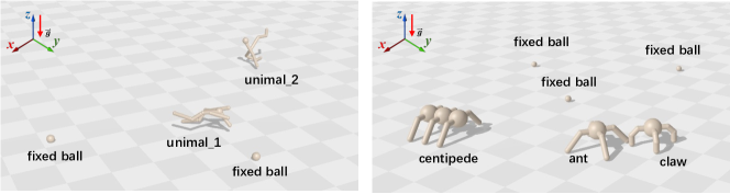
Figure 9: Team Reach Environments. Here, displaying 2_unimals and 3_ant_claw_centipede environments.

Team Reach

We expand the “Reach” task from a single-agent challenge to a collaborative “Team Reach” task, as shown in Figure 9. 1. Initial Conditions. Entities set $\Omega$ include $N$ agents and $M$ fixed balls, $N\geq M$. Within an area of radius $R$, we randomly position $N$ agents and $M$ fixed balls, also setting the initial orientations of the agents randomly. Specific details for $N$, $M$, $R$, and the agents’ morphology are provided in Table 4. 2. Termination. The goal of this task is for $M$ fixed balls to be simultaneously occupied by agents. An episode is considered successfully completed and terminates once this condition is fulfilled. 3. Reward. The designed reward structure comprises four components: a. Success Bonus: A significant sparse reward of 10,000 is awarded. b. Distance Reward: A dense reward to incentivize the achievement of the task objective. It is computed as $5\times\sum_{j=1}^{M}\exp(-\text{dist}_{j})$, where $\text{dist}_{j}$ represents the distance from the nearest agent to ball $j$. c. Moving Reward: Designed to motivate agents to move closer to any ball, it is quantified as $0.2\times\sum_{i=1}^{N}\sum_{j=1}^{M}\max(\vec{{\bm{v}}}_{i}\cdot(\vec{{\bm{p}}}_{j}-\vec{{\bm{p}}}_{i}),0)$. d. Control Cost: This penalty discourages agents from executing excessively large actions, and is calculated as $-0.2\times\sum_{i=1}^{N}\sqrt{\sum_{k=1}^{K_{i}}(a_{i,k})^{2}}$. Thus, the shared team reward is equal to the sum of the aforementioned rewards.

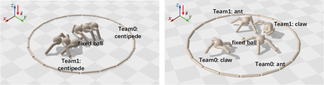
Figure 10: Team Sumo Environments. Here, displaying 1_centipede and 2_ant_claw environments.

Team Sumo

We evolve the “Sumo” task from a purely competitive challenge to a mixed cooperative-competitive “Team Sumo” task, as shown in Figure 10. 1. Initial Conditions. Entities set $\Omega$ comprise one fixed ball, $N$ agents forming Team 1, and another $M$ agents constituting Team 2. The sumo arena, a circle with radius $R$, has its center marked by the fixed ball. Around this fixed ball, within a radius of $R-1$, we randomly position $N$ agents from Team 1 and another $M$ from Team 2, ensuring each agent’s orientation is also randomized. Specific details for $N$, $M$, $R$, and the agents’ morphology are provided in Table 4. 2. Termination. The objective is for either Team 1 or Team 2 to win by having an opposing team’s agent disqualified, which occurs if it exceeds a distance $R$ from the fixed ball. The team with the disqualified agent loses, triggering the termination of the episode. 3. Reward. The reward designed for Team 1 (for Team 2, simply swap $N$ and $M$) is divided into five parts: a. Win Bonus: A sparse reward of 1000 for achieving the win condition. b. Lose Bonus: A sparse penalty of -1000 for the losing condition. c. Distance Reward: A dense reward to encourage achieving the task’s objective, computed as $5\times\exp(\text{dist}-R)$, where dist denotes the distance of the farthest agent from the opposing team to the fixed ball. d. Moving Reward: This motivates agents to move closer to any member of the opposing team, calculated as $5\times\sum_{i=1}^{N}\sum_{j=1}^{M}\max(\vec{{\bm{v}}}_{i}\cdot(\vec{{\bm{p}}}_{j}-\vec{{\bm{p}}}_{i}),0)$. e. Control Cost: A penalty for excessively large actions by agents, quantified as $-0.1\times\sum_{i=1}^{N}\sqrt{\sum_{k=1}^{K_{i}}(a_{i,k})^{2}}$. In line with the Exploration Curriculum suggested by Bansal et al. (2018), the shared team reward is calculated as $\alpha\times\text{dense reward}+(1-\alpha)\times\text{sparse reward}$, where $\alpha$ is a linear annealing factor. Agents train with the dense reward for 25% of the training epochs.

Table 4: Full list of environments used in this work.

Benchmark	Environment	Morphology	$N$	$M$	$R$ (meter)
Team Reach	1_ant	ant	1	1	5
	1_centipede	centipede	1	1	5
	2_ants	ant	2	2	3
	2_ant_claw	ant, claw	2	2	5
	2_unimals	unimal_1, unimal_2	2	2	5
	3_ant_claw_centipede	ant, claw, centipede	3	3	5
Team Sumo	1_centipede   vs   1_centipede	centipede	1	1	3
	2_ants   vs   2_ants	ant	2	2	3
	2_ant_claw   vs   2_ant_claw	ant, claw	2	2	3
	3_ants   vs   3_ants	ant	3	3	4

C.3 Baselines

We compare our method SHNN against mainstream neural networks, particularly MLP as utilized in  (Furuta et al., 2023), and a variant employing heading normalization technique, denoted as MLP+HN (Chen et al., 2023).

MLP

Our implementation of MLP consists of three linear layers. The middle two layers are activated by ReLU activation functions. The input layer is designed to accommodate the size of the observation space, while the output layer matches the dimensionality of the action space. The intermediate layers facilitate the non-linear transformation of input features. For specific hyperparameters, please refer to  Table 8.

MLP+HN

Heading Normalization technique has been widely utilized in the 3D RL literature. For instance, in morphology control, the presence of gravity allows for the normalization of state and action spaces in the heading (yaw) direction, as demonstrated in a recent work (Won et al., 2020, 2022; Chen et al., 2023). This heading normalization (HN) technique transforms the global coordinate frame into the LRF, enabling the input geometric information to be mapped to a rotation- and translation-invariant representation.

Specifically, we acquire the quaternion of the root body from the simulation environment and calculate the heading angle to construct the rotation matrix ${\bm{O}}_{i}$. This matrix is then multiplied by $\vec{{\bm{Z}}}_{i,k}$ to transform it into an invariant representation. Finally, all invariant representations are input into the MLP. It is noteworthy that Chen et al. (2023) discusses the limitations of this technique in their appendix.

Algorithm 1 Greedy Bipartite Matching for Task Assignment

  Input: $\vec{{\bm{p}}}_{i,1},i\in\Omega$, ${\mathcal{N}}$ {agents (Team0) set}, ${\mathcal{M}}$ {objects (Team1) set}

  Output: A local entity-level graph ${\mathcal{G}}=({\mathcal{V}},{\mathcal{E}})$

  Initialize the graph ${\mathcal{G}}$ with vertices ${\mathcal{V}}\leftarrow\Omega$ and edges ${\mathcal{E}}\leftarrow\emptyset$

  Initialize the assignment labels $\mathcal{C}\leftarrow\emptyset$

  Initialize distance matrix $D$ between ${\mathcal{N}}$ and ${\mathcal{M}}$

  for each $i\in{\mathcal{N}}$ and $j\in{\mathcal{M}}$ do

     $D[i,j]\leftarrow\|\vec{{\bm{p}}}_{j,1}-\vec{{\bm{p}}}_{i,1}\|_{2}$

  end for

  for each $j\in{\mathcal{M}}$ do

     $i=\operatorname*{arg\,min}_{k\in{\mathcal{N}}}D[k,j]$

     $D[i,:]\leftarrow\infty$ {Prevent re-matching}

     Add $(i,j)$ to ${\mathcal{E}}$: $\mathcal{C}(i)=i,\mathcal{C}(j)=i$

  end for

  return A local entity-level graph ${\mathcal{G}}=({\mathcal{V}},{\mathcal{E}})$

C.4 Task Assignment

Greedy Bipartite Matching Algorithm

The Greedy algorithm is a fundamental optimization algorithm, this part is about the process of applying the greedy matching algorithm to allocate a fixed ball (or an opposing agent) to each agent in the environments. Algorithm 1 provides a pseudo-code implementation of the Greedy Bipartite Matching algorithm.

C.5 Additional Ablations

Additional Ablations on Assignment

In the Team Sumo environments, task assignment yields limited improvement. This could be attributed to the environments’ complex mixture of cooperative and competitive dynamics, which are challenging to effectively decouple using bipartite matching methods, as demonstrated in  Figure 11.

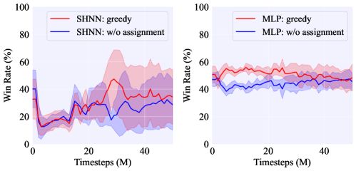
Figure 11: Additional Ablations on Assignment. Training and Evaluation Curves in 2_ants Team Sumo Environment.

Additional Ablations on Equivariance

In the Team Sumo environments, task assignment leads to the formation of local graphs composed of triplets of agents from both sides and a fixed ball, making it challenging to determine the specific goal orientation learned by equivariant networks. Consequently, our method was primarily compared against HNN+HN. The experimental outcomes align with the main text findings, as demonstrated in  Figure 12.

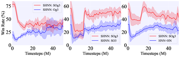
Figure 12: Additional Ablations on Equivariance. Training and Evaluation Curves in 2_ants Team Sumo Environment.

Importance of Local Symmetry

By comparing the red and blue lines in the left plot of Figure 11 and in the right plot of Figure 12, it becomes evident that in the Team Sumo environments, the impact of assignment is not as significant as that of equivariance. Therefore, careful design of assignment strategies is crucial to harness the advantages offered by equivariance effectively.

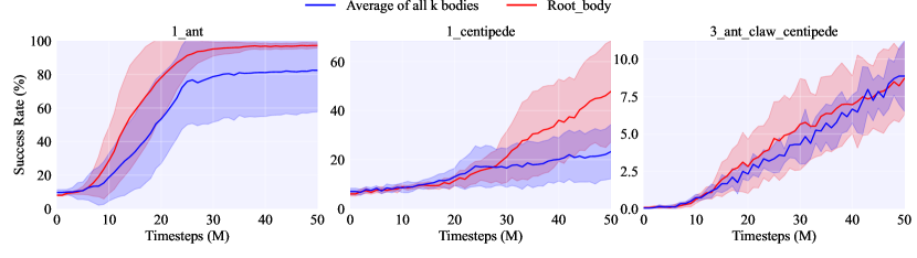
Figure 13: Additional Ablations on Entity Abstraction. Training and Evaluation Curves in 1_ant, 1_centipede, and 3_ant_claw_centipede Team Reach Environments.

Ablation Study on Entity Abstraction

The additional ablation study examines the effects of using different abstraction for each entity. Our hierarchical structure dictates a representative abstraction for each entity, and within RL environments, the reward is often contingent on the root body’s state. Utilizing the first (root) body as a representative aligns with the common computational practices in RL, focusing on the pivotal elements that influence agent behavior and reward structures. Moreover, representing entity-level information through the mean of all K bodies is a viable alternative, offering a more comprehensive local dynamic. The ablation study examines the effects of using the root body versus the average of all K bodies: Root body: $\vec{\bm{Z}}_{i}$ is assigned as $\vec{\bm{Z}}_{i,1}$, $\bm{h}_{i}$ is set as $[\bm{h}_{i,1},\vec{\bm{p}}_{i,1}^{z}]$, $\vec{\bm{Z}}_{ij}=[(\vec{\bm{p}}_{j,1}-\vec{\bm{p}}_{i,1}),\vec{\bm{Z}}_{i},\vec{\bm{Z}}_{j}]$, and $\bm{h}_{ij}=[\|\vec{\bm{p}}_{j,1}-\vec{\bm{p}}_{i,1}\|_{2},\bm{h}_{i},\bm{h}_{j}]$; Average of all $K$ bodies: $\vec{\bm{Z}}_{i}$ is assigned as $\frac{1}{K_{i}}\sum_{k=1}^{K_{i}}\vec{\bm{Z}}_{i,k}$, $\bm{h}_{i}$ is set as $[\frac{1}{K_{i}}\sum_{k=1}^{K_{i}}\bm{h}_{i,k},\frac{1}{K_{i}}\sum_{k=1}^{K_{i}}\vec{\bm{p}}_{i,k}^{z}]$,$\vec{\bm{Z}}_{ij}=[(\frac{1}{K_{j}}\sum_{k=1}^{K_{j}}\vec{\bm{p}}_{j,k}-\frac{1}{K_{i}}\sum_{k=1}^{K_{i}}\vec{\bm{p}}_{i,k}),\vec{\bm{Z}}_{i},\vec{\bm{Z}}_{j}]$, and $\bm{h}_{ij}=[\|\frac{1}{K_{j}}\sum_{k=1}^{K_{j}}\vec{\bm{p}}_{j,k}-\frac{1}{K_{i}}\sum_{k=1}^{K_{i}}\vec{\bm{p}}_{i,k}\|_{2},\bm{h}_{i},\bm{h}_{j}]$. The empirical results in Figure 13, particularly for the asymmetric 1_centipede scenario, reveal a significant performance gap, clearly demonstrating the superiority of using the root body’s state over the average of all K bodies.

C.6 Analyses of Morphology-shared Policy

We provide an extended example of our methodology applied to morphology tasks. Previous works have achieved generalization across agents with different morphologies using morphology-aware Graph Neural Networks (Wang et al., 2018; Huang et al., 2020).

Our variant, referred to as SHGNN, replaces the body-level MLP with body-level message passing. This adaptation enables the learning of a shared policy network across different agents.

First, we utilize the morphology topology information of each agent $i$ to construct a body-level inner-entity graph, denoted as ${\mathcal{G}}_{i}=({\mathcal{V}}_{i},{\mathcal{E}}_{i})$. For each body, $k\in{\mathcal{V}}_{i}$, input node features are initialized using the body’s state. Specifically, $\vec{{\bm{Z}}}_{k}$ is assigned as $\vec{{\bm{Z}}}_{i,k}$, and ${\bm{h}}_{k}$ is set as $[{\bm{h}}_{i,k},{\bm{h}}^{\prime}_{i},\vec{{\bm{p}}}_{i,k}^{z}]$, where [ ] is the stack along the last dimension and $\vec{{\bm{p}}}_{i,k}^{z}$ represents the projection of the coordinate $\vec{{\bm{p}}}_{i,k}$ onto the $z$-axis. In a body-level overview, we denote our body-level message passing as the function $\varphi_{b}$ that updates each body’s node features given the input node features of all body and graph connectivity:

$$\{(\vec{{\bm{Z}}}^{\prime}_{k},{\bm{h}}^{\prime}_{k})\}_{k=1}^{K_{i}} =\varphi_{b}\left(\{(\vec{{\bm{Z}}}_{k},{\bm{h}}_{k})\}_{k=1}^{K_{i}},{\mathcal{E}}_{i}\right).$$ (27)

Notably, the unfolding of $\varphi_{b}$ is similar to that of $\varphi_{o}$, and will not be elaborated further here.

For each agent $i$, the invariant actor policy $\pi_{\theta_{i}}$ is defined as

$$\pi_{\theta_{i}}=\{\pi_{\theta_{i,k}}\}_{k=2}^{K_{i}}=\{\sigma_{\pi}({\bm{O}}_{i}^{\top}\vec{{\bm{Z}}}^{\prime}_{k},{\bm{h}}^{\prime}_{k})\}_{k=2}^{K_{i}},$$ (28)

where $\sigma_{\pi}$ is a linear layer with bias. Here, $\pi_{\theta_{i}}\in{\mathbb{R}}^{2\times(K_{i}-1)}$ represents the location and scale parameters of a Normal Tanh Distribution for the $(K_{i}-1)$ actuators of agent $i$. Each actuator samples its corresponding torque $a_{i,k}\in[-1,1]$ from this distribution. The invariant critic value-function $V_{\phi}$ remains as described in the main text. Within the same team, different agents share the weight parameters of the body-level message passing.

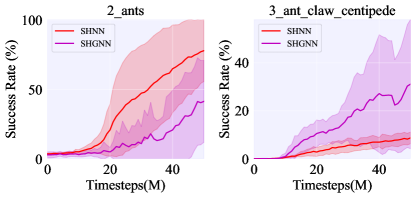
Figure 15: Analysis of Morphology-shared Policy. Training and Evaluation Curves in Team Reach Environments.

As observed in Figure 15, while body-level message passing struggles to learn effective control strategies for a single morphology (e.g., 2_ants), it interestingly excels in more complex, multi-morphological environments like 3_ant_claw_centipede. In such scenarios, knowledge sharing across different morphologies leads to mutual enhancement, significantly outperforming the body-level MLP approach. However, as indicated in Table 5, the implementation of message passing considerably slows down the training process.

C.7 Model Comparison: Parameters and Training Time

Table 5 compares the parameters and Training Wall Times of our model with several model variants in the 3_ant_claw_centipede Team Reach Environments. Here, total timesteps are 50M. Since Transformer and GNN can share parameters across different morphologies, they have fewer parameters.

Table 5: Comparison of Models in Terms of Parameters and Training Wall Time in 3_ant_claw_centipede Team Reach Environments.

Model	Parameters (M)	Training Wall Time (h)
MLP+HN	1.759	0.299$\pm$0.003
Transformer+HN	0.416	1.545$\pm$0.001
SHNN	0.772	1.302$\pm$0.012
SHTransformer	0.711	2.487$\pm$0.014
SHGNN	0.613	5.538$\pm$1.411

C.8 Equivariance Test

We conduct an experiment, as depicted in Figure 16, to evaluate the rotational generalization of both the baselines and our method. Training and evaluation are conducted in the fixed initial conditions of the 1_centipede and 2_ants Team Reach environments. Additionally, we conduct an evaluation with a 180° rotation of the entire scene. The results presented in Table 6, with detailed curves provided in Figure 17, illustrate that both our SHNN method and the MLP+HN approach exhibit stable performance pre- and post-rotation. Conversely, MLP demonstrates rotational generalization for symmetric morphologies, such as ants, yet entirely lacks this capability with asymmetric morphologies like centipedes, evidenced by the underline in Table 6 and the green line in the first plot of Figure 17. These results empirically validate that both our SHNN method and the HN approach are rotation equivariance, which can robustly generalize to unseen rotation transformations.

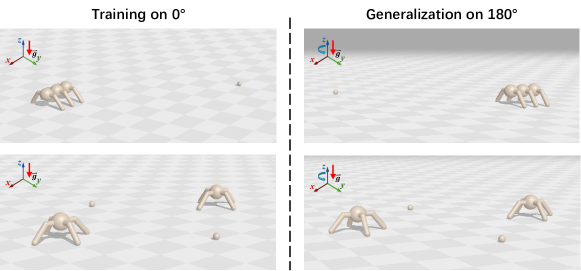
Figure 16: Equivariance Test Scenarios. Training are conducted in the fixed initial conditions, a generalization evaluation is conducted with a 180° rotation of the entire scene.

Table 6: Equivariance Test. We report Success Rate (%) on the final step in Team Reach Environments.

Methods	1_centipede		2_ants
	$0^{\circ}$	$180^{\circ}$	$0^{\circ}$	$180^{\circ}$
MLP	$\textbf{41.55}\pm 19.70$	$0.18\pm 0.22$	$44.00\pm 12.90$	$40.03\pm 12.03$
MLP+HN	$38.02\pm 24.98$	$37.92\pm 25.91$	$39.19\pm 12.85$	$38.60\pm 12.53$
SHNN	$40.23\pm 22.28$	$\textbf{41.39}\pm 21.89$	$\textbf{87.78}\pm 6.59$	$\textbf{87.84}\pm 6.42$

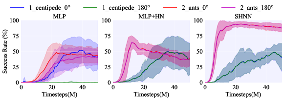
Figure 17: Equivariance Test. Training and Evaluation Curves in Team Reach Environments. MLP+HN and SHNN, by explicitly addressing local transformations, exhibit overlapping curves in equivariance tests.

C.9 Hyperparameters

Table 8 and Table 8 provide the hyperparameters needed to replicate our experiments. Code and Environments are available on our project page: https://alpc91.github.io/SMERL/.

Table 7: Hyperparameters of MAPPO.

Hyperparameter	Value
total_timesteps	Team Reach: 50M / Team Sumo: 20M
eval_frequency	50
num_envs	2048
action_repeat	1
batch_size	Team Reach: 1024 / Team Sumo: 128
reward_scaling	1.0
episode_length	1000
entropy_cost	1e-2
unroll_length	5
discounting	0.97
learning_rate	3e-4
num_minibatches	32
num_update_epochs	4
gradient_clipping	0.1
normalize_observations	True

Table 8: Hyperparameters of Network.

Module	Hyperparameters	Value
MLP	hidden_dim	256
	output_dim	$\pi$: $2\times(K_{i}-1)$ / $V$: 1
	# linear_layers	3
	activation	relu
Message Passing	hidden_dim	64
	vector_dim	32
	# MLP_layers	2
	activation	relu
	propagation_steps	2
Transformer	model_dim	128
	feedforward_dim	256
	# layers	3
	# heads	2
	activation	relu
	transformer_norm	LayerNorm
	condition_decoder	True
	positional_encoding	False

References

- Bansal et al. (2018) Bansal, T., Pachocki, J., Sidor, S., Sutskever, I., and Mordatch, I. Emergent complexity via multi-agent competition. In International Conference on Learning Representations, 2018.
- Bernstein et al. (2002) Bernstein, D. S., Givan, R., Immerman, N., and Zilberstein, S. The complexity of decentralized control of markov decision processes. Mathematics of operations research, 27(4):819–840, 2002.
- Bradbury et al. (2018) Bradbury, J., Frostig, R., Hawkins, P., Johnson, M. J., Leary, C., Maclaurin, D., Necula, G., Paszke, A., VanderPlas, J., Wanderman-Milne, S., and Zhang, Q. JAX: composable transformations of Python+NumPy programs, 2018. URL http://github.com/google/jax.
- Chen et al. (2023) Chen, R., Han, J., Sun, F., and Huang, W. Subequivariant graph reinforcement learning in 3d environment. In International Conference on Machine Learning. PMLR, 2023.
- Chen et al. (2018) Chen, T., Murali, A., and Gupta, A. Hardware conditioned policies for multi-robot transfer learning. In Advances in Neural Information Processing Systems, volume 31, 2018.
- Claus & Boutilier (1998) Claus, C. and Boutilier, C. The dynamics of reinforcement learning in cooperative multiagent systems. In Proceedings of the AAAI Conference on Artificial Intelligence, volume 1998, pp. 2, 1998.
- Cohen & Welling (2016) Cohen, T. S. and Welling, M. Group equivariant convolutional networks. In International Conference on Machine Learning, volume 48, pp. 2990–2999. PMLR, 2016.
- Cohen & Welling (2017) Cohen, T. S. and Welling, M. Steerable CNNs. In International Conference on Learning Representations, 2017.
- de Witt et al. (2020) de Witt, C. S., Peng, B., Kamienny, P.-A., Torr, P., Böhmer, W., and Whiteson, S. Deep multi-agent reinforcement learning for decentralized continuous cooperative control. arXiv preprint arXiv:2003.06709, 19, 2020.
- Deng et al. (2021) Deng, C., Litany, O., Duan, Y., Poulenard, A., Tagliasacchi, A., and Guibas, L. J. Vector neurons: A general framework for so (3)-equivariant networks. In Proceedings of the IEEE/CVF International Conference on Computer Vision, pp. 12200–12209, 2021.
- Deng et al. (2023) Deng, C., Lei, J., Shen, B., Daniilidis, K., and Guibas, L. Banana: Banach fixed-point network for pointcloud segmentation with inter-part equivariance. In Advances in Neural Information Processing Systems, 2023.
- D’Eramo et al. (2020) D’Eramo, C., Tateo, D., Bonarini, A., Restelli, M., Peters, J., et al. Sharing knowledge in multi-task deep reinforcement learning. In International Conference on Learning Representations, 2020.
- Devin et al. (2017) Devin, C., Gupta, A., Darrell, T., Abbeel, P., and Levine, S. Learning modular neural network policies for multi-task and multi-robot transfer. In IEEE International Conference on Robotics and Automation, pp. 2169–2176. IEEE, 2017.
- Dong et al. (2022) Dong, H., Wang, T., Liu, J., and Zhang, C. Low-rank modular reinforcement learning via muscle synergy. In Advances in Neural Information Processing Systems, 2022.
- Dresselhaus et al. (2007) Dresselhaus, M. S., Dresselhaus, G., and Jorio, A. Group theory: application to the physics of condensed matter. Springer Science & Business Media, 2007.
- Ellis et al. (2022) Ellis, B., Cook, J., Moalla, S., Samvelyan, M., Sun, M., Mahajan, A., Foerster, J. N., and Whiteson, S. Smacv2: An improved benchmark for cooperative multi-agent reinforcement learning. arXiv preprint arXiv:2212.07489, 2022.
- Foerster et al. (2016) Foerster, J., Assael, I. A., De Freitas, N., and Whiteson, S. Learning to communicate with deep multi-agent reinforcement learning. Advances in neural information processing systems, 29, 2016.
- Foerster et al. (2018) Foerster, J., Farquhar, G., Afouras, T., Nardelli, N., and Whiteson, S. Counterfactual multi-agent policy gradients. In Proceedings of the AAAI Conference on Artificial Intelligence, volume 32, 2018.
- Freeman et al. (2021) Freeman, C. D., Frey, E., Raichuk, A., Girgin, S., Mordatch, I., and Bachem, O. Brax - a differentiable physics engine for large scale rigid body simulation, 2021. URL http://github.com/google/brax.
- Fuchs et al. (2020) Fuchs, F., Worrall, D., Fischer, V., and Welling, M. Se(3)-transformers: 3d roto-translation equivariant attention networks. In Advances in Neural Information Processing Systems, volume 33, pp. 1970–1981. Curran Associates, Inc., 2020.
- Furuta et al. (2023) Furuta, H., Iwasawa, Y., Matsuo, Y., and Gu, S. S. A system for morphology-task generalization via unified representation and behavior distillation. In International Conference on Learning Representations, 2023.
- Godwin* et al. (2020) Godwin*, J., Keck*, T., Battaglia, P., Bapst, V., Kipf, T., Li, Y., Stachenfeld, K., Veličković, P., and Sanchez-Gonzalez, A. Jraph: A library for graph neural networks in jax., 2020. URL http://github.com/deepmind/jraph.
- Gu et al. (2021) Gu, S. S., Diaz, M., Freeman, D. C., Furuta, H., Ghasemipour, S. K. S., Raichuk, A., David, B., Frey, E., Coumans, E., and Bachem, O. Braxlines: Fast and interactive toolkit for rl-driven behavior engineering beyond reward maximization. arXiv preprint arXiv:2110.04686, 2021.
- Guan et al. (2024) Guan, H., Cai, G., and Xu, H. Automatic requirement dependency extraction based on integrated active learning strategies. Machine Intelligence Research, pp. 1–18, 2024.
- Gupta et al. (2022) Gupta, A., Fan, L., Ganguli, S., and Fei-Fei, L. Metamorph: Learning universal controllers with transformers. In International Conference on Learning Representations, 2022.
- Han et al. (2022) Han, J., Huang, W., Ma, H., Li, J., Tenenbaum, J. B., and Gan, C. Learning physical dynamics with subequivariant graph neural networks. In Advances in Neural Information Processing Systems, volume 35, pp. 26256–26268, 2022.
- Han et al. (2024) Han, J., Cen, J., Wu, L., Li, Z., Kong, X., Jiao, R., Yu, Z., Xu, T., Wu, F., Wang, Z., et al. A survey of geometric graph neural networks: Data structures, models and applications. arXiv preprint arXiv:2403.00485, 2024.
- Heek et al. (2023) Heek, J., Levskaya, A., Oliver, A., Ritter, M., Rondepierre, B., Steiner, A., and van Zee, M. Flax: A neural network library and ecosystem for JAX, 2023. URL http://github.com/google/flax.
- Hong et al. (2021) Hong, S., Yoon, D., and Kim, K.-E. Structure-aware transformer policy for inhomogeneous multi-task reinforcement learning. In International Conference on Learning Representations, 2021.
- Huang et al. (2020) Huang, W., Mordatch, I., and Pathak, D. One policy to control them all: Shared modular policies for agent-agnostic control. In International Conference on Machine Learning, pp. 4455–4464. PMLR, 2020.
- Huang et al. (2022) Huang, W., Han, J., Rong, Y., Xu, T., Sun, F., and Huang, J. Equivariant graph mechanics networks with constraints. In International Conference on Learning Representations, 2022.
- Iqbal & Sha (2019) Iqbal, S. and Sha, F. Actor-attention-critic for multi-agent reinforcement learning. In International Conference on Machine Learning, pp. 2961–2970. PMLR, 2019.
- Jeon et al. (2022) Jeon, J., Kim, W., Jung, W., and Sung, Y. Maser: Multi-agent reinforcement learning with subgoals generated from experience replay buffer. In International Conference on Machine Learning, pp. 10041–10052. PMLR, 2022.
- Jing et al. (2020) Jing, B., Eismann, S., Suriana, P., Townshend, R. J. L., and Dror, R. Learning from protein structure with geometric vector perceptrons. In International Conference on Learning Representations, 2020.
- Joshi et al. (2023) Joshi, C. K., Bodnar, C., Mathis, S. V., Cohen, T., and Lio, P. On the expressive power of geometric graph neural networks. In International Conference on Machine Learning. PMLR, 2023.
- Kraemer & Banerjee (2016) Kraemer, L. and Banerjee, B. Multi-agent reinforcement learning as a rehearsal for decentralized planning. Neurocomputing, 190:82–94, 2016.
- Kuba et al. (2021) Kuba, J. G., Chen, R., Wen, M., Wen, Y., Sun, F., Wang, J., and Yang, Y. Trust region policy optimisation in multi-agent reinforcement learning. In International Conference on Learning Representations, 2021.
- Kurin et al. (2020) Kurin, V., Igl, M., Rocktäschel, T., Boehmer, W., and Whiteson, S. My body is a cage: the role of morphology in graph-based incompatible control. In International Conference on Learning Representations, 2020.
- Lechner et al. (2023) Lechner, M., Yin, L., Seyde, T., Wang, T.-H., Xiao, W., Hasani, R., Rountree, J., and Rus, D. Gigastep-one billion steps per second multi-agent reinforcement learning. In Advances in Neural Information Processing Systems, 2023.
- Littman (1994) Littman, M. L. Markov games as a framework for multi-agent reinforcement learning. In Machine learning proceedings 1994, pp. 157–163. Elsevier, 1994.
- Liu et al. (2018) Liu, S., Lever, G., Merel, J., Tunyasuvunakool, S., Heess, N., and Graepel, T. Emergent coordination through competition. In International Conference on Learning Representations, 2018.
- Liu et al. (2022) Liu, S., Lever, G., Wang, Z., Merel, J., Eslami, S. A., Hennes, D., Czarnecki, W. M., Tassa, Y., Omidshafiei, S., Abdolmaleki, A., et al. From motor control to team play in simulated humanoid football. Science Robotics, 7(69):eabo0235, 2022.
- Lowe et al. (2017) Lowe, R., Tamar, A., Harb, J., Pieter Abbeel, O., and Mordatch, I. Multi-agent actor-critic for mixed cooperative-competitive environments. In Advances in Neural Information Processing Systems, volume 30, 2017.
- Luo et al. (2022) Luo, S., Li, J., Guan, J., Su, Y., Cheng, C., Peng, J., and Ma, J. Equivariant point cloud analysis via learning orientations for message passing. In Proceedings of the IEEE/CVF Conference on Computer Vision and Pattern Recognition, pp. 18932–18941, 2022.
- Mnih et al. (2015) Mnih, V., Kavukcuoglu, K., Silver, D., Rusu, A. A., Veness, J., Bellemare, M. G., Graves, A., Riedmiller, M., Fidjeland, A. K., Ostrovski, G., et al. Human-level control through deep reinforcement learning. Nature, 518(7540):529–533, 2015.
- Mnih et al. (2016) Mnih, V., Badia, A. P., Mirza, M., Graves, A., Lillicrap, T., Harley, T., Silver, D., and Kavukcuoglu, K. Asynchronous methods for deep reinforcement learning. In International Conference on Machine Learning, pp. 1928–1937. PMLR, 2016.
- Oliehoek et al. (2016) Oliehoek, F. A., Amato, C., et al. A concise introduction to decentralized POMDPs, volume 1. Springer, 2016.
- Pathak et al. (2019) Pathak, D., Lu, C., Darrell, T., Isola, P., and Efros, A. A. Learning to control self-assembling morphologies: a study of generalization via modularity. In Advances in Neural Information Processing Systems, volume 32, 2019.
- Rashid et al. (2018) Rashid, T., Samvelyan, M., Schroeder, C., Farquhar, G., Foerster, J., and Whiteson, S. Qmix: Monotonic value function factorisation for deep multi-agent reinforcement learning. In International Conference on Machine Learning, pp. 4295–4304. PMLR, 2018.
- Rutherford et al. (2023) Rutherford, A., Ellis, B., Gallici, M., Cook, J., Lupu, A., Ingvarsson, G., Willi, T., Khan, A., de Witt, C. S., Souly, A., Bandyopadhyay, S., Samvelyan, M., Jiang, M., Lange, R. T., Whiteson, S., Lacerda, B., Hawes, N., Rocktaschel, T., Lu, C., and Foerster, J. N. Jaxmarl: Multi-agent rl environments in jax. arXiv preprint arXiv:2311.10090, 2023.
- Samvelyan et al. (2019) Samvelyan, M., Rashid, T., Schroeder de Witt, C., Farquhar, G., Nardelli, N., Rudner, T. G., Hung, C.-M., Torr, P. H., Foerster, J., and Whiteson, S. The starcraft multi-agent challenge. In International Conference on Autonomous Agents and Multiagent Systems, pp. 2186–2188, 2019.
- Satorras et al. (2021) Satorras, V. G., Hoogeboom, E., and Welling, M. E (n) equivariant graph neural networks. In International Conference on Machine Learning, pp. 9323–9332. PMLR, 2021.
- Schulman et al. (2017) Schulman, J., Wolski, F., Dhariwal, P., Radford, A., and Klimov, O. Proximal policy optimization algorithms. arXiv preprint arXiv:1707.06347, 2017.
- Silver et al. (2016) Silver, D., Huang, A., Maddison, C. J., Guez, A., Sifre, L., Van Den Driessche, G., Schrittwieser, J., Antonoglou, I., Panneershelvam, V., Lanctot, M., et al. Mastering the game of go with deep neural networks and tree search. Nature, 529(7587):484–489, 2016.
- Spelke (2022) Spelke, E. S. What babies know: Core knowledge and composition volume 1, volume 1. Oxford University Press, 2022.
- Sunehag et al. (2018) Sunehag, P., Lever, G., Gruslys, A., Czarnecki, W. M., Zambaldi, V., Jaderberg, M., Lanctot, M., Sonnerat, N., Leibo, J. Z., Tuyls, K., et al. Value-decomposition networks for cooperative multi-agent learning based on team reward. In International Conference on Autonomous Agents and MultiAgent Systems, pp. 2085–2087, 2018.
- Thomas et al. (2018) Thomas, N., Smidt, T., Kearnes, S., Yang, L., Li, L., Kohlhoff, K., and Riley, P. Tensor field networks: Rotation-and translation-equivariant neural networks for 3d point clouds. arXiv preprint arXiv:1802.08219, 2018.
- van der Pol et al. (2020) van der Pol, E., Worrall, D., van Hoof, H., Oliehoek, F., and Welling, M. Mdp homomorphic networks: Group symmetries in reinforcement learning. In Advances in Neural Information Processing Systems, volume 33, pp. 4199–4210, 2020.
- Villar et al. (2021) Villar, S., Hogg, D. W., Storey-Fisher, K., Yao, W., and Blum-Smith, B. Scalars are universal: Equivariant machine learning, structured like classical physics. In Advances in Neural Information Processing Systems, volume 34, pp. 28848–28863, 2021.
- Wang et al. (2024) Wang, L., Chen, R., Wang, Y., Sun, F., Wang, X., Kai, S., Fu, G., Zhang, J., and Huang, W. Equivariant local reference frames for unsupervised non-rigid point cloud shape correspondence. arXiv preprint arXiv:2404.00959, 2024.
- Wang et al. (2018) Wang, T., Liao, R., Ba, J., and Fidler, S. Nervenet: Learning structured policy with graph neural networks. In International Conference on Learning Representations, 2018.
- Wen et al. (2022) Wen, M., Kuba, J., Lin, R., Zhang, W., Wen, Y., Wang, J., and Yang, Y. Multi-agent reinforcement learning is a sequence modeling problem. Advances in Neural Information Processing Systems, 35:16509–16521, 2022.
- Won et al. (2020) Won, J., Gopinath, D., and Hodgins, J. A scalable approach to control diverse behaviors for physically simulated characters. ACM Transactions on Graphics (TOG), 39(4):33–1, 2020.
- Won et al. (2022) Won, J., Gopinath, D., and Hodgins, J. Physics-based character controllers using conditional vaes. ACM Transactions on Graphics (TOG), 41(4):1–12, 2022.
- Worrall et al. (2017) Worrall, D. E., Garbin, S. J., Turmukhambetov, D., and Brostow, G. J. Harmonic networks: Deep translation and rotation equivariance. In Proceedings of the IEEE/CVF Conference on Computer Vision and Pattern Recognition, pp. 5028–5037, 2017.
- Xiong et al. (2023) Xiong, Z., Beck, J., and Whiteson, S. Universal morphology control via contextual modulation. In International Conference on Machine Learning. PMLR, 2023.
- Xu et al. (2023) Xu, Z., Bai, Y., Zhang, B., Li, D., and Fan, G. Haven: Hierarchical cooperative multi-agent reinforcement learning with dual coordination mechanism. In Proceedings of the AAAI Conference on Artificial Intelligence, volume 37, pp. 11735–11743, 2023.
- Yin et al. (2024) Yin, Q., Yu, T., Shen, S., Yang, J., Zhao, M., Ni, W., Huang, K., Liang, B., and Wang, L. Distributed deep reinforcement learning: A survey and a multi-player multi-agent learning toolbox. Machine Intelligence Research, pp. 1–20, 2024.
- Yu et al. (2022) Yu, C., Velu, A., Vinitsky, E., Gao, J., Wang, Y., Bayen, A., and Wu, Y. The surprising effectiveness of ppo in cooperative multi-agent games. In Advances in Neural Information Processing Systems, volume 35, pp. 24611–24624, 2022.